Latent Hierarchical Model for Activity Recognition

Abstract

We present a novel hierarchical model for human activity recognition. In contrast to approaches that successively recognize actions and activities, our approach jointly models actions and activities in a unified framework, and their labels are simultaneously predicted. The model is embedded with a latent layer that is able to capture a richer class of contextual information in both state-state and observation-state pairs. Although loops are present in the model, the model has an overall linear-chain structure, where the exact inference is tractable. Therefore, the model is very efficient in both inference and learning. The parameters of the graphical model are learned with a Structured Support Vector Machine (Structured-SVM). A data-driven approach is used to initialize the latent variables; therefore, no manual labeling for the latent states is required. The experimental results from using two benchmark datasets show that our model outperforms the state-of-the-art approach, and our model is computationally more efficient.

I Introduction

The use of robots as companions to help people in their daily life is currently being widely studied. Numerous studies have focused on providing people with physical [1], cognitive [2] or social [3] support. To achieve this, a fundamental and necessary task is to recognize human activities. For example, to decide when to offer physical support, a robot needs to recognize that a person is walking. To decide whether to remind people to continue drinking, a robot needs to recognize past drinking activities. To determine whether a person is lonely, a robot needs to detect interactions between people. In this paper, we propose a hierarchical approach to model human activities.

(a)

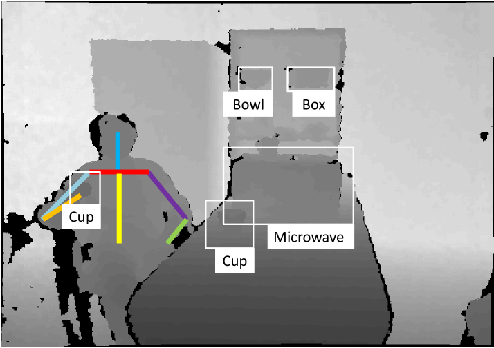
(b)

Figure 1: An example that shows a robot helping people in an elderly home. LABEL:sub@fig:cover_girl_color Care-O-bot 3 offers water to the elderly after detecting that the elderly resident has not drunk any water for a long time. LABEL:sub@fig:cover_girl_depth In this work, an RGB-D sensor is used to recognize human activities. This work is built upon existing methods in object recognition, object localization, and human skeleton tracking. Object and human skeleton information are combined as the input of our model to infer human activities.

Different types of sensors have been applied to the task of activity recognition [4, 5]. Kasteren et al.[6] adopt a set of simple sensors, i.e. , pressure, contact, and motion sensors, to recognize daily activities of people in a smart home. Hu et al.[7] use a ceiling-mounted color camera to recognize human postures, and the postures are recognized based on still images. Recently, RGB-D sensors, such as the Microsoft Kinect and ASUS Xtion Pro, have become popular in activity recognition because they can capture 2.5D data using structured light, thereby allowing researchers to extract a rich class of depth features for activity recognition. In this work, we equip a robot with an RGB-D sensor to collect sequences of activity data, from which we extract object locations and human skeleton points, as shown in Fig. 1. Based on these observations, our task is to estimate activities as well as sequences of composing actions.

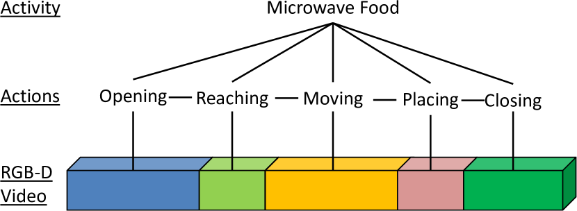
Figure 2: An illustration of the activity hierarchy. The input video is represented as a spatial-temporal volume. The bottom layer shows a video that is discretized into multiple temporal segments for modeling, and spatial-temporal features are extracted from each temporal segment. In the middle layer, actions are recognized from the input features with one atomic activity per segment. In the second layer, the activities are described in terms of the sub-level activity sequence. The un-directed links in the graph represent the inter-dependency between layers. Note that the video segments may not have the same length; thus, a segmentation method needs to be applied.

We distinguish between activities and actions as follows. Actions are the atomic movements of a person that relate to at most one object in the environment, e.g. , reaching, placing, opening, and closing. Most of these actions are completed in a relatively short period of time. In contrast, activities refer to a complete sequence that is composed of different actions. For example, microwaving food is an activity that can be decomposed into a number of actions such as opening the microwave, reaching for food, moving food, placing food, and closing the microwave. The relation between actions and activities is illustrated in Fig. 2.

The recognition of actions is usually formulated as a sequential prediction problem [8] (see Fig. 2). In this approach, the RGB-D video is first divided into smaller video segments so that each segment contains approximately one action. This can be accomplished either by manual annotation or by automated temporal segmentation based on motion features. Spatio-temporal features are extracted for each segment. For real-world tasks in HRI, it is desirable to recognize activities at a higher level whereby the activities are usually performed over a longer duration. The combination of actions and activities forms a sequential model with a hierarchy (Fig. 2).

Most previous work addresses activity and action recognition as separate tasks [9, 10, 8], i.e. , the action labels need to be inferred before the activity labels are predicted. In contrast, in this paper, we jointly model actions and activities in a unified framework, where the activity and action labels are learned simultaneously. Our experimental evaluation demonstrates that this framework is beneficial when compared to separate recognition. This can be intuitively understood by considering the case of learning actions: the activity label provides additional constraints to the action labels, which can result in a better estimation of the actions, and vice versa.

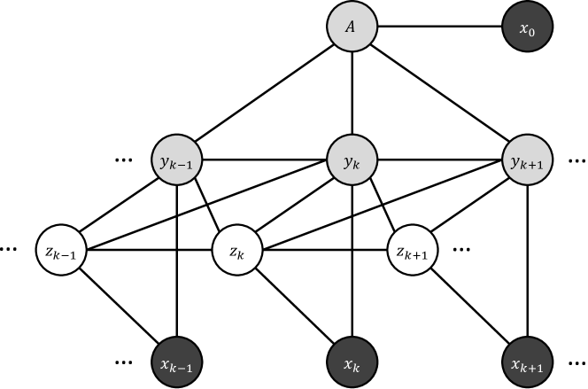
Figure 3: The graphical representation of our model. Nodes that represent the observations $\boldsymbol{x}$, which are observed both in training and testing, are rendered in black. $\boldsymbol{y}$ refers to action nodes, and $\mathcal{A}$ is the corresponding activity label of the sequence. Both are in gray because they are only observed during training and not testing. White nodes $\boldsymbol{z}$ refer to the latent variables, which are unknown either in training or testing. They are used to represent the hidden sub-level semantics among consecutive actions. Note that $\boldsymbol{x_{k}}$, $\boldsymbol{y_{k}}$, $\boldsymbol{z_{k}}$ are fully connected in our model as are the temporal transitions of action-latent pairs. Therefore, the model enables a richer representation of a activity hierarchy. $\boldsymbol{x}_{0}$ represents the set of global features.

Fig. 3 is a graphical representation of our approach. The proposed model of this paper is based on our previous work [11], wherein we recognize the sequence of actions using Conditional Random Fields (CRFs). The model is augmented with a layer of latent nodes to enrich the model’s expressiveness. For simplicity, we use latent variables to refer to the variables in the hidden layer, which are unknown both during training and testing. Labels, in contrast, are known during training but are latent during testing. The latent variables are able to capture such a difference and are able to model the rich variations of the actions. One can imagine that the latent variables represent sub-types of the actions: e.g. , for the action opening, we are able to model the difference between opening a bottle and opening a door using latent variables.

For each temporal segment, we preserve the full connectivity among observations, latent variables, and action nodes, thus avoiding making inappropriate conditional independence assumptions. We describe an efficient method of applying exact inference in our graph, whereby collapsing the latent states and target states allows our graphical model to be considered as a linear-chain structure. Applying exact inference under such a structure is very efficient. We use a max-margin approach for learning the parameters of the model. Benefiting from the discriminative framework, our method needs not model the correlation between the input data, thus providing us with a natural way of data fusion.

The model was evaluated using the RGB-D data from two different benchmark datasets[12, 9]. The results are compared with a number of the state-of-the-art approaches [12, 9, 10, 11, 8]. The results show that our model performs better than the state-of-the-art approaches, and the model is more efficient in terms of inference.

In summary, the contribution of this paper is a novel Hidden CRF model for jointly predicting activities and their sub-level actions, which outperforms the state of the art both in terms of predictive performance and in computational cost. Our software is open source and freely accessible at http://ninghanghu.eu/activity_recognition.html.

In this paper, we address the following research questions:

• How important is it to add an activity hierarchy to the model?

• How important is it to add the latent layer to the model?

• How important is it to joint model actions and activities?

• How does our model compare with state-of-the-art approaches?

• How well can the model be generalized to a new problem?

The remainder of the paper is organized as follows. We describe the related work in Section II. We formalize the model and present the objective function in Section III. The inference and learning algorithms are introduced in Section IV and Section V. We show the implementation details and the comparison of the results with the state-of-the-art approach in Section VI.

II Related Work

The previous works can be categorized into two methodologies. The first methodology divides the approaches based on the hierarchical layout of the model, i.e. , whether the model contains a single layer or multiple layers. The second methodology is based on the nature of the learning method, i.e. , whether the method is discriminative or generative.

II-A Single-layer Approach and Hierarchical Approach

Human activity recognition is a key component for HRI, particularly for the re-ablement of the elderly [13]. Depending on the complexity and duration of activities, activity recognition approaches can be separated into two categories [14]: single-layer approaches and hierarchical approaches. Single-layer approaches [15, 16, 17, 18, 19, 20, 21, 22, 23] refer to methods that are able to directly recognize human activities from the data without defining any activity hierarchy. Usually, these activities are both simple and short; therefore, no higher level layers are required. Typical activities in this category include walking, waiting, falling, jumping and waving. Nevertheless, in the real world, activities are not always as simple as these basic actions. For example, the activity of preparing breakfast may consist of multiple actions such as opening a fridge, getting a salad and making coffee. Typical hierarchical approaches [9, 11, 24, 25, 26] first estimate the sub-level actions, and then, the high-level activity labels are inferred based on the action sequences.

Sung et al. [12] proposed a hierarchical maximum entropy Markov model that detects activities from RGB-D videos. They consider the actions as hidden nodes that are learned implicitly. Recently, Koppula et al. [9] presented an interesting approach that models both activities and object affordance as random variables. The object affordance label is defined as the possible manners in which people can interact with an object, e.g. , reachable, movable, and eatable. These nodes are inter-connected to model object-object and object-human interactions. Nodes are connected across the segments to enable temporal interactions. Given a test video, the model jointly estimates both human activities and object affordance labels using a graph-cut algorithm. After the actions are recognized, the activities are estimated using a multi-class SVM. In this paper, we build a hierarchical approach that jointly estimates actions and activities from the RGB-D videos. The inference algorithm is more efficient compared with graph-cut methods.

II-B Generative Models and Discriminative Models

Many different graphical models, e.g. , Hidden Markov Models (HMMs) [27, 12], Dynamic Bayesian Networks (DBNs) [28], linear-chain CRFs [29], loopy CRFs [9], Semi-Markov Models [6], and Hidden CRFs [30, 31], have been applied to the recognition of human activities. The graphical models can be divided into two categories: generative models [27, 12] and discriminative models [9, 6, 7]. The generative models require making assumptions concerning both the correlation of data and how the data are distributed given the activity state. This is risky because the assumptions may not reflect the true attributes of the data. The discriminative models, in contrast, only focus on modeling the posterior probability regardless of how the data are distributed. The robotic and smart environment scenarios are usually equipped with a combination of multiple sensors. Some of these sensors may be highly correlated both in the temporal and spatial domain, e.g. , a pressure sensor on a mattress and a motion sensor above a bed. In these scenarios, the discriminative models provide a natural way of data fusion for human activity recognition.

The linear-chain Conditional Random Field (CRF) is one of the most popular discriminative models and has been used for many applications. Linear-chain CRFs are efficient models because the exact inference is tractable. However, these models are limited because they cannot capture the intermediate structures within the target states [32]. By adding an extra layer of latent variables, the model allows for more flexibility and therefore can be used for modeling more complex data. The names of these models, including Hidden-unit CRF [33], Hidden-state CRF [32] or Hidden CRF [31], are inter-changeable in the literature.

Koppula et al. [9] present a model for the temporal and spatial interactions between humans and objects in loopy CRFs. More specifically, they develop a model that has two types of nodes for representing the action labels of the human and the object affordance labels of the objects. Human nodes and object nodes within the same temporal segment are fully connected. Over time, the nodes are transited to the nodes with the same type. The results show that by modeling the human-object interaction, their model outperforms the earlier work in [12] and [34]. The inference in the loopy graph is solved as a quadratic optimization problem using the graph-cut method [35]. Their inference method, however, is less efficient compared with the exact inference in a linear-chain structure because the graph-cut method requires multiple iterations before convergence; more iterations are usually preferred to ensure that a good solution is obtained.

Another study [36] augments an additional layer of latent variables to the linear-chain CRFs. They explicitly model the new latent layer to represent the durations of activities. In contrast to [9], Tang et al. [36] solve the inference problem by reforming the graph into a set of cliques so that the exact inference can be efficiently solved using dynamic programming. In their model, the latent variables and the observation are assumed to be conditionally independent given the target states.

Our work is different from the previous approaches in terms of both the utilized graphical model and the efficiency of inference. First, similar to [36], our model also uses an extra latent layer. However, instead of explicitly modeling the latent variables, we directly learn the latent variables from the data. Second, we do not make conditional independence assumptions between the latent variables and the observations. Instead, we add one extra edge between them to make the local graph fully connected. Third, although our graph also presents many loops, as in [9], we are able to transform the cyclic graph into a linear-chain structure wherein the exact inference is tractable. The exact inference in our graph only requires two passes of messages across the linear chain structure, which is substantially more efficient than the method in [9]. Finally, we model the interaction between the human and the objects at the feature level instead of modeling the object affordance as target states. Therefore, the parameters are learned and are directly optimized for activity recognition rather than for making the joint estimation of both object affordance and human activity. Because we apply a data-driven approach to initializing the latent variables, hand labeling of the object affordance is not necessary in our model. Our results show that the model outperforms the state-of-the-art approaches on the CAD$120$ dataset [9].

III Modeling Activity Hierarchy

The graphical model of our proposed system is illustrated in Fig. 3. Let $\boldsymbol{x}=\{\boldsymbol{x}_{1},\boldsymbol{x}_{2},\dots,\boldsymbol{x}_{K}|\boldsymbol{x}_{k}\in\mathbb{R}^{D}\}$ be the sequence of observations, where $K$ is the total number of temporal segments in the video. Our goal is to predict the most likely underlying action sequence $\boldsymbol{y}=\{y_{1},y_{2},\dots,y_{K}|y_{k}\in\mathcal{Y}\}$ and its corresponding activity label $A\in\mathcal{H}$ based on the observations. We define $\boldsymbol{x}_{0}$ as the global features that are extracted from $\boldsymbol{x}$.

Each observation $\boldsymbol{x}_{k}$ is a feature vector extracted from the segment $k$. The form of $\boldsymbol{x}_{k}$ is quite flexible. $\boldsymbol{x}_{k}$ can be collections of data from different sources, e.g. , simple sensor readings, human locations, human poses, and object locations. Some of these observations may be highly correlated with each other, e.g. , wearable accelerate meters and motion sensors would be highly correlated. Because of the discriminative nature of our model, we do not need to model such correlation among the observations.

We define $\boldsymbol{z}=\{z_{1},z_{2},\dots,z_{K}|z_{k}\in\mathcal{Z}\}$ to be the latent variables in the model. The latent variables, which are implicitly learned from the data, can be considered as modeling the sub-level semantics of the actions. For clarity, one could imagine that $y_{k}=1$ refers to the action opening. Then, the joint $(y_{k}=1,z_{k}=1)$ can describe opening a microwave, and $(y_{k}=1,z_{k}=2)$ can describe opening a bottle. Note that these two sub-types of opening actions differ greatly in the observed videos. However, the latent variables allow us to capture large variations in the same action.

Next, we will formulate our model in terms of these defined variables. For simplicity, we assume that there are in total $N_{y}$ actions and $N_{a}$ activities to be recognized, and let us define $N_{z}$ as the cardinality of the latent variable.

III-A Potential Function

Our model contains five types of potentials that together form the potential function.

The first potential measures the score of making an observation $\boldsymbol{x}_{k}$ with a joint-state assignment $(z_{k},y_{k}$). We define $\Phi(\boldsymbol{x}_{k})$ to be the function that maps the input data into the feature space. $\boldsymbol{w}$ is a matrix that contains model parameters.

$$\psi_{1}(y_{k},z_{k},\boldsymbol{x}_{k};\boldsymbol{w}_{1})=\boldsymbol{w}_{1}(y_{k},z_{k})\cdot\Phi(\boldsymbol{x}_{k})$$ (1)

where $\boldsymbol{w}_{1}\in\mathbb{R}^{\mathcal{Y}\times\mathcal{Z}\times D}$ and $\boldsymbol{w}_{1}(y_{k},z_{k})$ is the concatenation of the parameters that corresponds to $y_{k}$ and $z_{k}$.

This potential models the full connectivity among $y_{k}$, $z_{k}$ and $\boldsymbol{x}_{k}$ and avoids making any conditional independence assumptions. It is more accurate to have such a structure because $z_{k}$ and $\boldsymbol{x}_{k}$ may not be conditionally independent over a given $y_{k}$ in many cases. Let us consider the aforementioned example. Knowing that the action is opening, whether the latent state refers to opening a microwave or opening a bottle depends on how the opening action is performed in the observed video, i.e. , the latent state and the observation are inter-dependent given the action label.

The second potential measures the score of coupling $y_{k}$ with $z_{k}$. The score can be considered as either the bias entry of (1) or the prior of seeing the joint state $(y_{k},z_{k})$.

$$\psi_{2}(y_{k},z_{k};\boldsymbol{w}_{2})=\boldsymbol{w}_{2}(y_{k},z_{k})$$ (2)

where $\boldsymbol{w}_{2}$ represents the parameter of the second potential with $\boldsymbol{w}_{2}\in\mathbb{R}^{\mathcal{Y}\times\mathcal{Z}}$.

The third potential characterizes the transition score from the joint state $(y_{k-1},z_{k-1})$ to $(y_{k},z_{k})$. Comparing with the normal transition potentials [31], our model leverages the latent variable $z_{k}$ for modeling richer contextual information over consecutive temporal segments. Our model not only contain the transition between the action states but also captures the sub-level context using the latent variables.

$$\psi_{3}(y_{k-1},z_{k-1},y_{k},z_{k};\boldsymbol{w}_{3})=\boldsymbol{w}_{3}(y_{k-1},z_{k-1},y_{k},z_{k})$$ (3)

where the potential is parameterized by $\boldsymbol{w}_{3}\in\mathbb{R}^{\mathcal{Y}\times\mathcal{Z}\times\mathcal{Y}\times\mathcal{Z}}$.

The fourth potential models the compatibility among consecutive action pairs and the activity.

$$\psi_{4}(y_{k-1},y_{k},A;\boldsymbol{w}_{4})=\boldsymbol{w}_{4}(y_{k-1},y_{k},A)$$ (4)

where $\boldsymbol{w}_{4}\in\mathbb{R}^{\mathcal{Y}\times\mathcal{Y}\times\mathcal{H}}$ and $\boldsymbol{w}_{4}(y_{k-1},y_{k},A)$ is a scalar that reflects the compatibility between the transition of an action and the activity label.

The last potential models the compatibility between the activity label $A$ and the global features $\boldsymbol{x}_{0}$.

$$\psi_{5}(A,\boldsymbol{x}_{0};\boldsymbol{w}_{5})=\boldsymbol{w}_{5}(A)\cdot\Phi(\boldsymbol{x}_{0})$$ (5)

where the parameters $\boldsymbol{w}_{5}\in\mathbb{R}^{\mathcal{H}}$ can be interpreted as a global filter that favors certain combinations of $\boldsymbol{x}_{0}$ and $A$.

Summing all potentials over the entire sequence, we can write the final potential function of our model as follows:

$$F(A,\boldsymbol{y},\boldsymbol{z},\boldsymbol{x};\boldsymbol{w})=\sum_{k=1}^{K}\boldsymbol{w}_{1}(y_{k},z_{k})\cdot\Phi(\boldsymbol{x}_{k})+\sum_{k=1}^{K}\boldsymbol{w}_{2}(y_{k},z_{k})$$

$$+\sum_{k=2}^{K}\boldsymbol{w}_{3}(y_{k-1},z_{k-1},y_{k},z_{k})+\sum_{k=2}^{K}\boldsymbol{w}_{4}(y_{k-1},y_{k},A)$$

$$+\boldsymbol{w}_{5}(A)\cdot\Phi(\boldsymbol{x}_{0})$$ (6)

The potential function evaluates the matching score between the joint states $(A,\boldsymbol{y},\boldsymbol{z})$ and the input $(\boldsymbol{x}$, $\boldsymbol{x}_{0})$. The score equals the un-normalized joint probability in the log space. The objective function can be rewritten in a more general linear form $F(\boldsymbol{y},\boldsymbol{z},\boldsymbol{x};\boldsymbol{w})=\boldsymbol{w}\cdot\Psi(\boldsymbol{y},\boldsymbol{z},\boldsymbol{x})$. Therefore, the model is in the class of log-linear models.

Note that it is not necessary to explicitly model the latent variables; rather, the latent variables can be automatically learned from the training data. Theoretically, the latent variables can represent any form of data, e.g. , time duration and action primitives, as long as the data can be used to facilitate the task. The optimization of the latent model, however, may converge to a local minimum. The initialization of the random variables is therefore of great importance. We compare three initialization strategies in this paper. Details of the latent variable initialization will be discussed in Section VI-B1.

One may notice that our graphical model has many loops, which in general makes the exact inference intractable. Because our graph complies with the semi-Markov property, we will now show how we benefit from such a structure to obtain efficient inference and learning.

IV Inference

Given the graph and the parameters, inference is used to find the most likely joint state $(A,\boldsymbol{y},\boldsymbol{z})$ that maximizes the objective function.

$$(A^{*},\boldsymbol{y}^{*},\boldsymbol{z}^{*})=\operatorname*{argmax}_{(A,\boldsymbol{y},\boldsymbol{z})\in\mathcal{H}\times\mathcal{Y}\times\mathcal{Z}}F(A,\boldsymbol{y},\boldsymbol{z},\boldsymbol{x};\boldsymbol{w})$$ (7)

Generally, solving (7) is an NP-hard problem that requires the evaluation of the objective function over an exponential number of state sequences. Exact inference is preferable because it is guaranteed to find the global optimum. However, the exact inference usually can only be applied efficiently when the graph is acyclic. In contrast, approximate inference is more suitable for loopy graphs but may take longer to converge and is likely to obtain a local optimum. Although our graph contains loops, we can transform the graph into a linear-chain structure, in which the exact inference becomes tractable. If we collapse the latent variable $z_{k}$ with $y_{k}$ and $A$ into a single factor, the edges among $z_{k}$, $y_{k}$ and $A$ become the internal factor of the new node, and the transition edges collapse into a single transition edge. This results in a typical linear-chain CRF, where the cardinality of the new nodes is $N_{y}\times N_{z}\times N_{A}$. In the linear-chain CRF, the exact inference can be efficiently performed using dynamic programming [37].

Using the chain property, we can write the following recursion procedure for computing the maximal score over all possible assignments of $\boldsymbol{y}$, $\boldsymbol{z}$ and A.

$$V_{k}(A,y_{k},z_{k})= \boldsymbol{w}_{1}(y_{k},z_{k})\cdot\Phi(\boldsymbol{x}_{k})+\boldsymbol{w}_{2}(y_{k},z_{k})$$

$$+\max_{(y_{k-1},z_{k-1})\in\mathcal{Y}\times\mathcal{Z}}\{\boldsymbol{w}_{3}(y_{k-1},z_{k-1},y_{k},z_{k})$$

$$+\boldsymbol{w}_{4}(y_{k-1},y_{k},A)+V_{k-1}(A,y_{k-1},z_{k-1})\}$$ (8)

The above function is evaluated iteratively across the entire sequence. For each iteration, we record the joint state $(y_{k-1},z_{k-1})$ that contributes to the max. When the last segment is computed, the optimal assignment of segment $K$ can be computed as

$$A^{*},y_{K}^{*},z_{K}^{*}=\operatorname*{argmax}_{A,y_{K},z_{K}}V_{K}(A,y_{K},z_{K})+\boldsymbol{w}_{5}(A)\cdot\Phi(\boldsymbol{x}_{0})$$ (9)

Knowing the optimal assignment at $K$, we can track back the best assignment in the previous time step $K-1$. The process continues until all $\boldsymbol{y}^{*}$ and $\boldsymbol{z}^{*}$ have been assigned, i.e. , the inference problem in (7) is solved.

Computing (IV) once involves $O(N_{y}N_{z})$ computations. In total, (IV) needs to be evaluated for all possible assignments of $(y_{k},z_{k},N_{A})$; thus, it is computed $N_{y}N_{z}$ times. The total computational cost is, therefore, $O(N_{y}^{2}\,N_{z}^{2}\,N_{A}K)$. Such computation is manageable when $N_{y}N_{z}$ is not very large, which is usually the case for the tasks of activity recognition.

Next, we show how we can learn the parameters using the max-margin approach.

V Learning

We use the max-margin approach for learning the parameters in our graphical model. Given a set of N training examples, $\langle\boldsymbol{x}^{(n)},\boldsymbol{y}^{(n)},A^{(n)}\rangle$ $(n=1,2,\cdots,N)$, we would like to learn the model parameters $\boldsymbol{w}$ that can produce the activity label $A$ and action labels $\boldsymbol{y}$ given a new test input $\boldsymbol{x}$. Note that both activities and action labels are observed during training. The latent variables $\boldsymbol{z}$ are unobserved and will be automatically inferred from the training process.

The goal of learning is to find the optimal model parameters $\boldsymbol{w}$ that minimize the objective function. A regularization term is used to avoid over-fitting.

$$\min_{\boldsymbol{w}}\left\{\frac{1}{2}\|\boldsymbol{w}\|^{2}+C\sum_{i=1}^{N}\Delta(\boldsymbol{y}^{(i)},\widehat{\boldsymbol{y}},A^{(i)},\widehat{A})\right\}$$ (10)

where $C$ is a normalization constant that is used to provide a balance between the model complexity and fitting rate.

The loss function $\Delta(\boldsymbol{y}^{(i)},\widehat{\boldsymbol{y}},A^{(i)},\widehat{A})$ measures the cost of making incorrect predictions. $\widehat{\boldsymbol{y}}$ and $\widehat{A}$ are the most likely action and activity labels that are computed from (7). The loss function in (11) returns zero when the prediction is exactly the same as the ground truth; otherwise, it counts the number of disagreed elements.

$$\Delta(\boldsymbol{y}^{(i)},\widehat{\boldsymbol{y}},A^{(i)},\widehat{A})=\lambda\,\mathds{1}(A^{(i)}=\widehat{A})+\frac{1}{K}\sum_{k=1}^{K}\mathds{1}(y_{k}^{(i)}=\widehat{y}_{k})$$ (11)

where $\mathds{1}(\cdot)$ is an indicator function and $0\leq\lambda\leq 1$ is a scalar weight that balances between the two loss terms.

This object function can be viewed as a generalized form of our previous work [11], where we recognize only the sequence of actions. This is can be performed by simply setting $\lambda$ to $0$ and leaving the graphical structure unchanged. The learning framework then only tracks the incorrectly predicted actions, regardless of the activities.

Directly optimizing (10) is not possible because the loss function involves computing the $\operatorname*{argmax}$ in (7). Following [38] and [39], we substitute the loss function in (10) by the margin rescaling surrogate, which serves as an upper-bound of the loss function.

$$\min_{\boldsymbol{w}}\{\frac{1}{2}\|\boldsymbol{w}\|^{2}+C\sum_{i=1}^{n}\max_{A,\boldsymbol{y},\boldsymbol{z}}[\Delta(\boldsymbol{y}^{(i)},\boldsymbol{y},A^{(i)},A)+$$

$$F(\boldsymbol{x}^{(i)},\boldsymbol{y},A,\boldsymbol{z},\boldsymbol{w})]-C\sum_{i=1}^{n}\max_{\boldsymbol{z}}F(\boldsymbol{x}^{(i)},\boldsymbol{y}^{(i)},A^{(i)},\boldsymbol{z},\boldsymbol{w})\}$$ (12)

The second term in (12) can be solved using the augmented inference, i.e. , by plugging in the loss function as an extra factor in the graph, the term can be solved in the same way as the inference problem using (7). Similarly, the third term of (12) can be solved by adding $\boldsymbol{y}^{(i)}$ and $A^{(i)}$ as the evidence into the graph and then applying inference using (7). Because the exact inference is tractable in our graphical model, both of the terms can be computed very efficiently.

Note that (12) is the summation of a convex and concave function. This can be solved with the Concave-Convex Procedure (CCCP) [40]. By substituting the concave function with its tangent hyperplane function, which serves as an upper bound of the concave function, the concave term is transformed into a linear function. Thus, (12) becomes convex again.

We can rewrite (12) in the form of minimizing a function subject to a set of constraints by adding slack variables

$$\min_{\boldsymbol{w},\boldsymbol{\xi}}\{\frac{1}{2}\|\boldsymbol{w}\|^{2}+ C\sum_{i=1}^{n}\xi_{i}\}$$ (13)

$$s.t.~{}\forall i\in\{1,2,\dots,n\},\forall y\in\mathcal{Y}$$

$$F(\boldsymbol{x}^{(i)},\boldsymbol{y}^{(i)},A^{(i)},\boldsymbol{z}^{*},\boldsymbol{w})- F(\boldsymbol{x}^{(i)},\boldsymbol{y},A,\boldsymbol{z},\boldsymbol{w})$$

$$\geq\Delta(\boldsymbol{y}^{(i)},\boldsymbol{y},A^{(i)},A)-\xi_{i}$$

where $\boldsymbol{z}^{*}$ is the most likely latent states that are inferred given the training data.

Note that there are an exponential number of constraints in (13). This can be solved using the cutting-plane method [41].

Another intuitive method of understanding the CCCP algorithm is to consider the algorithm as one that solves the learning problem with incomplete data using Expectation-Maximization (EM) [42]. In our training data, the latent variables are unknown. We can start by initializing the latent variables. Once we have the latent variables, the data become complete. Then, we can use the standard Structured-SVM to learn the model parameters (M-step). Subsequently, we can update the latent states again using the parameters that are learned (E-step). The iteration continues until convergence.

The CCCP algorithm decreases the objective function in each iteration. However, the algorithm cannot guarantee a global optimum. To avoid being trapped in a local minimum, we present three different initialization strategies, and details will be presented in Section VI-B1.

Note that the inference algorithm is extensively used in learning. Because we are able to compute the exact inference by transforming the loopy graph into a linear-chain graph, our learning algorithm is much faster and more accurate compared with the other approaches with approximate inference.

VI Experiments and Results

We implemented the proposed model, denoted as full model, along with its three variations. Specifically, the first model recognizes only low-level actions, the second model recognizes high-level activities, and the third model recognizes activities based on actions. All models were evaluated on two different datasets. The results from the different models were compared to gain insight into our research questions (in Section I). The full model is also shown to outperform the state-of-the-art methods.

VI-A Datasets

The methods were evaluated on two benchmark datasets, i.e. , CAD-60 [12] and CAD-120 [9]. Both of the datasets contain sequences of color and depth images that were collected by a RGB-D sensor. Skeleton joints of the person are obtained using OpenNI.

The two datasets are quite different from each other; therefore, they can be used to test the generalizability of our methods. The CAD-60 dataset consists of 12 human action labels and no activity labels. The actions include rinsing mouth, brushing teeth, wearing contact lens, talking on the phone, drinking water, opening pill container, cooking (chopping), cooking (stirring), talking on couch, relaxing on couch, writing on white board, and working on computer. These actions are performed by 4 different subjects in 5 different environments, i.e. , a kitchen, a bedroom, a bathroom, a living room, and an office. In total, the dataset includes approximately 60 videos, and each video contains one action label. In contrast, the CAD-120 dataset [9] contains 126 RGB-D videos, and each video contains one activity and a sequence of actions. There are in total 10 activities defined in the dataset, including making cereal, taking medicine, stacking objects, unstacking objects, microwaving food, picking up objects, cleaning objects, taking food, arranging objects, and having a meal. Fig. 4 shows various sample images of these activities. In addition, the dataset also consists of 10 sub-level actions, i.e. , reaching, moving, pouring, eating, drinking, opening, placing, closing, scrubbing, and null. The objects in CAD-120 are automatically detected as in [9], and the locations of the objects are also provided by the dataset.

(a) Arranging Objects

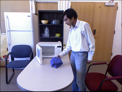
(b) Cleaning Objects

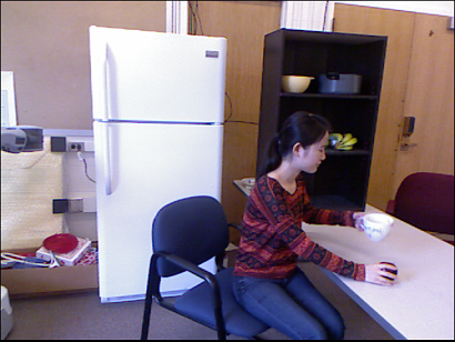
(c) Having Meal

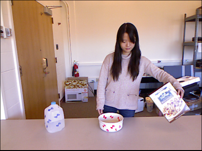
(d) Making Cereal

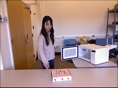
(e) Microwaving Food

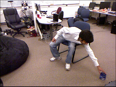
(f) Picking Objects

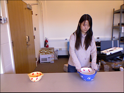
(g) Stacking Objects

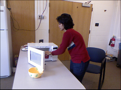
(h) Taking Food

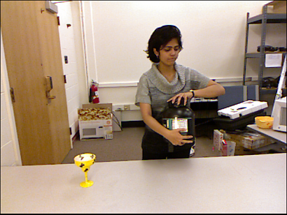
(i) Taking Medicine

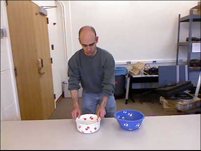
(j) Unstacking Objects

Figure 4: Sample images from the CAD-120 dataset. The images illustrate 10 different activities.

The two datasets are very challenging in the following aspects. a) The activities in the dataset are performed by four different actors. The actors behave quite differently, e.g. , in terms of being left or right handed, being viewed from a front view or side view, and sitting or standing. b) There is a large variation even for the same action, e.g. , the action opening can refer to opening a bottle or opening the microwave. Although both of actions have the same label, they appear significantly different from each other in the video. c) Partial or full occlusion is also a very challenging aspect for this dataset. e.g. in certain videos, the actors’ legs are completely occluded by the table, and objects are frequently occluded by the other objects. This makes it difficult to obtain accurate object locations as well as body skeletons; therefore, the generated data are noisy.

A number of recent approaches [9, 10, 11, 8, 12] have been evaluated on these two datasets; therefore, the results can be directly compared. To ensure a fair comparison, the same input features are extracted following [9]. Specifically, we have object features $\phi_{o}(\boldsymbol{x}_{k})\in\mathbb{R}^{180}$, object-object interaction features $\phi_{oo}(\boldsymbol{x}_{k})\in\mathbb{R}^{200}$, object-subject relation features $\phi_{oa}(\boldsymbol{x}_{k})\in\mathbb{R}^{400}$, and the temporal object and subject features $\phi_{t}(\boldsymbol{x}_{k})\in\mathbb{R}^{200}$. For CAD-120, we extract the complete set of features from the object locations, which are provided by the dataset. For CAD-60 dataset, only skeletal features are extracted because there is no object information. These features are concatenated into a single feature vector, which is considered as the observation of one action segment, i.e. , $\Phi(\boldsymbol{x}_{k})$.

VI-B Implemented Models

In this section, we describe the three baseline models in detail, followed by the introduction of the full model. Note that all of the models were first evaluated on the CAD-120 dataset. To test the generalizability of the model, the same experiments are repeated using the CAD-60 dataset. Note that the CAD-60 dataset contains no activity labels, but it has additional labels to indicate the environments. In our experiments, we treat these additional labels as if they were activities; thus, the model structure is left unchanged compared with the experiments on CAD-120. The only difference is that we jointly model the actions with the environments instead of the activities.

VI-B1 Recognize Only Low-level Actions

The first model is adopted from our previous work [11], which predicts action labels based on the video sequence. This model is a single-layer approach that only contains the low-level layer of nodes. By setting the weight $\lambda$ to zero, the model focuses only on predicting correct action labels regardless of the activity label; therefore, the model can be considered as a special case of the full model. The parameters of this model are learned with the Structured-SVM framework [38]. We use the margin rescaling surrogate as the loss. For optimization, we use the 1-slack algorithm (primal), as described in [43].

To initialize the latent states on CAD-120, we adopt three different initialization strategies. a) Random initialization. The latent states are randomly selected. b) A data-driven approach. We apply clustering on the input data $\boldsymbol{x}$. The number of clusters is set to be the same as the number of latent states. We run K-means for 10 times. Then, we choose the best clustering results based on minimal within-cluster distances. The labels of the clusters are assigned as the initial latent states. c) Initialized by Object affordance. The object affordance labels are provided by the CAD-120 dataset, which are used for training in [9]. We apply the K-means clustering upon the affordance labels. As the affordance labels are categorical, we use 1-of-N encoding to transform the affordance labels into binary values for clustering. The CAD-60 dataset do not contain affordance labels, therefore the latent variables are initialized only with the data-driven approach.

VI-B2 Recognize Only High-level Activities

The second model contains only a single layer for recognizing activities, i.e. , we disregard the layer of actions; instead, we learn a direct mapping from video features to activity labels. Similar to the first model, the parameters are learned with the Structured-SVM, but the model contains no transition.

VI-B3 Recognize Activities Based on Action Sequences

This approach is built upon the first baseline. Based on the inferred action labels, we learn a model to classify activities. We extract unigram and bigram features based on the action sequence as well as the occlusion features. The model parameters are estimated with a variation of multi-class SVM, where the latent layer is augmented in the model. In this approach, the actions and activities are recognized in succession.

VI-B4 Joint Estimation of Activity and Actions using Hierarchical Approach (full model)

This approach refers to the proposed model of the paper. Instead of successively recognizing actions and activities, our model uses a hierarchical framework to make joint predictions over both activity and action labels.

We compare two different segmentation methods to the videos in the CAD-120 dataset. In the first method, we use the ground truth segmentation, which is manually annotated. For the second segmentation, we apply a motion-based approach, i.e. , we extract the spatial-temporal features for all the frames, and similar frames are grouped together using a graph-based approach to form segments. For CAD-60, we apply uniform segmentation as in [9] to enable a fair comparison with other methods.

The above methods were evaluated on both the CAD-120 and CAD-60 datasets. Because the two datasets are quite different from each other, they can be used to test how the results can be generalized to new data. The performance of these methods on both datasets is reported in Section VI-D.

VI-C Evaluation Criteria

Our model was evaluated with 4-fold cross-validation. The folds are split based on the 4 subjects. To choose the hyper-parameters, i.e. , the number of latent states and segmentation methods, we used two subjects for training, one subject for validation and one subject for testing. Once the optimal hyper-parameters are chosen, the performance of the model during testing is measured by another cross-validation process, i.e. , training using videos of 3 persons and testing on a new person. Each cross-validation is performed 3 times. To observe the generalization of our model across different data sets, the results are averaged across the folds. In this paper, the accuracy (classification rate), precision, recall and F-score are reported to enable a comparison of the results. In the CAD-120 dataset, more than half of the instances are reaching and moving. Therefore, we consider precision and recall to be relatively better evaluation criteria than accuracy because they remain meaningful despite class imbalance.

VI-D Results and Analysis

TABLE I: Performance of Activity and Action Recognition during testing on the CAD-120 Dataset. The results are reported in terms of Accuracy, Precision, Recall and F-Score. The standard error is also reported.

Ground Truth Segmentation
Methods	Action				Activity
	Accuracy	Precision	Recall	F1-Score	Accuracy	Precision	Recall	F-Score
Single layer	-	-	-	-	$74.2\pm 5.1$	$78.5\pm 4.7$	$73.3\pm 5.1$	$75.8\pm 4.9$
Koppula et al. [9]	$86.0\pm 0.9$	$84.2\pm 1.3$	$76.9\pm 2.6$	$80.4\pm 1.7$	$84.7\pm 2.4$	$85.3\pm 2.0$	$84.2\pm 2.5$	$84.7\pm 2.2$
Koppula et al. [10]	$89.3\pm 0.9$	$87.9\pm 1.8$	$84.9\pm 1.5$	$86.4\pm 1.6$	$93.5\pm 3.0$	$95.0\pm 2.3$	$93.3\pm 3.1$	$94.1\pm 2.6$
Hu et al. [8][11]	$87.0\pm 0.9$	$89.2\pm 2.3$	$83.1\pm 1.2$	$85.5\pm 1.6$	$90.0\pm 2.9$	$92.8\pm 2.3$	$89.7\pm 3.0$	$91.2\pm 2.5$
Our Model (no latent)	$87.2\pm 0.8$	$87.4\pm 1.5$	$85.0\pm 1.4$	$86.2\pm 1.4$	$87.9\pm 1.5$	$91.9\pm 0.7$	$87.5\pm 1.6$	$89.7\pm 1.0$
Our Model (full)	$89.7\pm 0.6$	$90.2\pm 0.7$	$88.2\pm 0.6$	$89.2\pm 0.6$	$93.6\pm 2.7$	$95.2\pm 2.0$	$93.3\pm 2.8$	$94.2\pm 2.3$
Motion-based Segmentation
Methods	Action				Activity
	Accuracy	Precision	Recall	F-Score	Accuracy	Precision	Recall	F-Score
Single layer	-	-	-	-	$75.0\pm 5.3$	$79.0\pm 4.9$	$74.2\pm 5.5$	$76.5\pm 5.2$
Koppula et al. [9]	$68.2\pm 0.3$	$71.1\pm 1.9$	$62.2\pm 4.1$	$66.4\pm 2.6$	$80.6\pm 1.1$	$81.8\pm 2.2$	$80.0\pm 1.2$	$80.9\pm 1.6$
Koppula et al. [10]	$70.3\pm 0.6$	$74.8\pm 1.6$	$66.2\pm 3.4$	$70.2\pm 2.2$	$83.1\pm 3.0$	$87.0\pm 3.6$	$82.7\pm 3.1$	$84.8\pm 3.3$
Hu et al. [8][11]	$70.0\pm 0.3$	$70.3\pm 0.5$	$67.8\pm 0.2$	$69.0\pm 0.3$	$79.0\pm 6.2$	$86.4\pm 4.9$	$78.8\pm 5.9$	$82.4\pm 4.4$
Our Model (no latent)	$67.1\pm 0.4$	$69.1\pm 1.2$	$65.6\pm 1.5$	$67.3\pm 1.8$	$79.0\pm 2.0$	$80.4\pm 2.7$	$78.5\pm 2.0$	$79.4\pm 2.3$
Our Model (full)	$70.2\pm 1.2$	$71.1\pm 1.8$	$69.9\pm 1.9$	$70.5\pm 1.9$	$85.2\pm 1.4$	$90.3\pm 1.9$	$84.7\pm 1.5$	$87.4\pm 1.7$

TABLE II: Test Performance on the CAD-60 dataset with Uniform Segmentation. The standard error is also reported.

Methods	Action				Environment
	Accuracy	Precision	Recall	F-Score	Accuracy	Precision	Recall	F-Score
Single layer	-	-	-	-	$50.0\pm 2.8$	$63.0\pm 2.5$	$52.8\pm 2.2$	$57.5\pm 2.3$
Hu et al. [8][11]	$66.5\pm 4.3$	$71.1\pm 2.6$	$67.1\pm 3.7$	$67.7\pm 3.4$	$60.0\pm 1.5$	$71.0\pm 2.5$	$62.1\pm 1.8$	$63.0\pm 2.1$
Our Model (full)	$74.4\pm 4.0$	$80.3\pm 4.4$	$81.0\pm 1.6$	$80.7\pm 2.9$	$60.6\pm 0.5$	$74.7\pm 2.7$	$62.5\pm 1.0$	$68.6\pm 1.9$

In this section, we report the experimental results and compare the performance of different models. Table I shows the performance of all the models during testing on the CAD-120 dataset. Both the performances of the action and activity recognition are reported. For comparison, the results of both ground-truth segmentation and motion-based segmentation are reported. Table II shows the performance during testing on the CAD-60 dataset.

Next, we analyze the results while referring to our research questions posed in Section I.

Importance of hierarchical model. In Table I, Single Layer refers to the second baseline approach, wherein we learn a direct mapping from video-level features to activity labels. There is no intermediate layer of labels. The Single Layer approach achieves an average performance of over 70% in both segmentation methods but with a large standard error of approximately 5%. In contrast, the other hierarchical approaches outperform the Single Layer approach by at least 10 percentage points when using ground-truth segmentation and 5 percentage points when using motion-based segmentation. By incorporating the layer of action labels, we can see significant improvements in terms of recognizing activities. Therefore, temporal information, such as transitions between actions, is a very important aspect of activity recognition.

Table II shows the results using the CAD-60 dataset under similar experiment settings; however, the goal here is to predict actions together with the environment. We can see that the F-score of the environment prediction is increased by over 11 percentage points when using the hierarchical approach (full model), which is significantly better than the single-layer approach. The hierarchical approaches also exhibit significant improvements in terms of precision and recall. The increase in the mean is over 6 percentage points, with a reduced standard error rate.

Importance of embedding the latent layer. To demonstrate the importance of using latent variables, we compare the proposed model (full model) to the model without augmenting latent variables (no latent). Table I shows that the full model outperforms no latent in terms of recognition of both actions and activities. Notably, after adding the latent variable, the precision and recall for activity is increased by over $4$ and $5$ percentage points, respectively, using ground-truth segmentation. When using motion-based segmentation, the performance of full model for an activity is increased by $10$ percentage points in terms of precision and $6$ percentage points in terms of recall. The improvement is significant after using latent variables. Note that the no latent model is a special case of the full model, i.e. , no latent is equivalent to the full model when there is only one latent state. Here, we list these models separately to illustrate the effect of using multiple latent states. In contrast, Table II only shows the performance of the full model because the model starts overfitting the data when more than one latent states are applied to the model, i.e. , no latent (latent=1) achieves the best performance. From this, we can see that the model is quite flexible and that it can be used to fit data with varying levels of complexity by simply adjusting the number of latent states in the model.

Importance of jointly modeling activity and action. Hu et al. [8][11] in Table I refers to a combination of the first and third baseline approaches, where we used a two-step approach to successively recognize actions and activities. This method shows significant improvement over the Single layer approach. However, their approach is significantly outperformed by our proposed hierarchical method (full model) using both segmentation methods. Notably, for activity recognition, the F-score is increased by 3 percentage points using our proposed model, with an increase of 4 percentage points in terms of precision and 6 percentage points in terms of recall. For action recognition, the performance gain in terms of F-score is approximately 3.7 percentage points and includes significant improvements in both precision and recall. This is because the full model allows the interaction between the low-level and high-level layers during both learning and inference, and labels with the hierarchy are jointly estimated when making predictions. Similar results were found using the CAD-60 dataset, see Table II. We note that the performance is largely increased when using the full model. The F-score is increased by 3 percentage points for predicting action and environment labels.

Comparison with the state-of-the-art approaches. The proposed method was evaluated on both the CAD-60 and CAD-120 datasets to provide a comparison with the state-of-the-art methods.

To be comparable with the other approaches, following [12, 9], we conduct similar experiments on the CAD-60 dataset, where we group the actions based on their environment labels and a separate model is learned and tested for each of the groups. The results of these experiments are reported in Table III. We note that our model outperforms [12] in all five environments. Compared with the state of the art [9], our model outperforms [12] and [9] on most of the environments. On average, the precision of our model is the same as in [9], and the recall of the model outperforms [9] by over $8$ percentage points, achieving $80.8\%$ for precision and $80.1\%$ for recall. The average F-Score is over $4\%$ percentage points better than in [9].

TABLE III: Performance on the CAD-60 dataset. Note that in these experiments, the actions are grouped based on their locations, and a separate model is trained and tested based the ENVIRONMENT label; therefore, the results are different from Table II. The results are reported in terms of Precision (P. %), Recall (R. %), and F-Score (F. %). The standard error of our model is reported.

Methods	Bathroom			Bedroom			Kitchen			Living Room			Office			Average
	P. %	R. %	F. %	P. %	R. %	F. %	P. %	R. %	F. %	P. %	R. %	F. %	P. %	R. %	F. %	P. %	R. %	F. %
Sung et al. [12]	$72.7$	$65.0$	$68.9$	$76.1$	$59.2$	$67.7$	$64.4$	$47.9$	$64.7$	$52.6$	$45.7$	$49.2$	$73.8$	$59.8$	$66.8$	$67.9$	$55.5$	$61.7$
Koppula et al. [9]	88.9	$61.1$	$75.0$	$73.0$	$66.7$	$69.9$	96.4	$85.4$	90.9	$69.2$	$68.7$	$69.0$	$76.7$	$75.0$	$75.9$	80.8	$71.4$	$76.1$
Our Model	$77.6$	81.5	78.1	81.8	76.9	78.8	$88.2$	92.0	$90.1$	80.6	75.9	78.3	81.7	75.1	78.4	80.8	80.1	80.5
Our Model (std. err.)	$(6.9)$	$(5.7)$	$(6.3)$	$(2.7)$	$(3.5)$	$(3.1)$	$(5.2)$	$(2.6)$	$(3.9)$	$(6.6)$	$(7.3)$	$(7.0)$	$(5.4)$	$(6.2)$	$(5.8)$	$(5.4)$	$(5.1)$	$(5.3)$

Table I compares the performance of different approaches on the CAD-120 datasets. Similar to [8], Koppula et al. [10] use a two-step approach to infer high-level activity labels only after the actions are estimated. Benefiting from the joint estimation of action and activity, our full model outperforms the state-of-the-art models in terms of both action and activity recognition tasks. Notably, using ground-truth segmentation, the F-score is improved by approximately 4 percentage points for recognizing actions. Based on motion segmentation, the activity recognition performance is improved by over 2 percentage points in terms of F-Score.

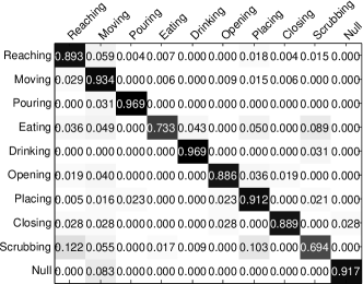
(a)

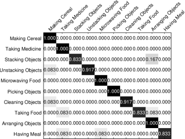
(b)

Figure 5: Confusion matrix over different action LABEL:sub@fig:confmat_actions and activity LABEL:sub@fig:confmat_activity classes. Rows are ground-truth labels, and columns are the detections.

Fig. 5 shows the confusion matrix of both the action and activity classification results. The most difficult action class is scrubbing. This task is sometimes confused with reaching and placing. The overall performance of the activity recognition is very good, with most of the activities being correctly classified. The more difficult case is to distinguish between “stacking objects” and “arranging objects”. Overall, we can see that high values are found on the diagonal using both segmentation methods, which demonstrates the good performance of our system.

VII Conclusion

In this paper, we present a hierarchical approach that simultaneously recognizes actions and activities based on RGB-D data. The interactions between actions and activities are captured by a Hidden-state CRF framework. In this framework, we use the latent variables to exploit the underlying structures of actions. The prediction is based on the joint interaction between activities and actions, which is in contrast to the traditional approach, which only focuses on one of them. Our results show a significant improvement when using the hierarchical model compared to using the single-layered approach. The results also demonstrate the effectiveness of adding a latent layer to the model and the importance of jointly estimating actions and activities. Finally, we show that the proposed hierarchical approach outperforms the state-of-the-art methods on two benchmark datasets.

Ninghang Hu is currently a Ph.D. candidate in the Informatics Institute at the University of Amsterdam, The Netherlands. His research interests are in machine learning and robot vision, with a focus on human activity recognition and data fusion. He received his M.Sc. in Artificial Intelligence from the same university in 2011 and his B.Sc. in Software Engineering from Xidian University, China in 2008. In 2011, he was a trainee at TNO (the Netherlands Organisation for Applied Scientific Research).

Gwenn Englebienne received the Ph.D. degree in computer science from the University of Manchester in 2009. He has since focused on automated analysis of human behavior at the University of Amsterdam, where he has developed computer vision techniques for tracking humans across large camera networks and machine learning techniques to model human behavior from networks of simple sensors. His main research interests are in models of human behavior, especially their interaction with other humans, with the environment, and with intelligent systems.

Zhongyu Lou received his B.Sc. and M.Sc. degrees from Xidian University, Xi’An, China, in 2008 and 2011, respectively. He is currently pursuing his Ph.D. degree at the Intelligent Systems Lab Amsterdam, University of Amsterdam, The Netherlands. His main research interests include computer vision, image processing and machine learning.

Ben Kröse is a Professor of “Ambient Robotics” at the University of Amsterdam and a Professor of “Digital Life” at the Amsterdam University of Applied Science. His research focuses on robotics and interactive smart devices, which are expected to be widely applied to smart services to ensure the health, safety, well-being, security and comfort of users. In the fields of artificial intelligence and autonomous systems, he has published 35 papers in scientific journals, edited 5 books and special issues, and submitted more than 100 conference papers. He owns a patent on multi-camera surveillance. He is a member of the IEEE, Dutch Pattern Recognition Association and Dutch AI Association.

References

- [1] Y. Miyake, “Interpersonal synchronization of body motion and the walk-mate walking support robot,” IEEE Transactions on Robotics, vol. 25, pp. 638–644, 2009.
- [2] J. Pineau, M. Montemerlo, M. Pollack, N. Roy, and S. Thrun, “Towards robotic assistants in nursing homes: Challenges and results,” in Robotics and Autonomous Systems, vol. 42, 2003, pp. 271–281.
- [3] K. Wada and T. Shibata, “Living with seal robots - Its sociopsychological and physiological influences on the elderly at a care house,” in IEEE Transactions on Robotics, vol. 23, 2007, pp. 972–980.
- [4] O. D. Lara and M. a. Labrador, “A Survey on Human Activity Recognition using Wearable Sensors,” IEEE Communications Surveys & Tutorials, pp. 1–18, 2012.
- [5] M. S. Ryoo, “Human activity prediction: Early recognition of ongoing activities from streaming videos,” in Proceedings of the IEEE international conference on computer vision (ICCV). IEEE, 2011, pp. 1036–1043.
- [6] T. L. M. van Kasteren, G. Englebienne, and B. Kröse, “Activity recognition using semi-markov models on real world smart home datasets,” Journal of Ambient Intelligence and Smart Environments, vol. 2, no. 3, pp. 311–325, 2010.
- [7] N. Hu, G. Englebienne, and B. Kröse, “Posture Recognition with a Top-view Camera,” in Proceedings of the IEEE/RSJ International Conference on Intelligent Robots and Systems (IROS). IEEE, 2013, pp. 2152–2157.
- [8] ——, “A Two-layered Approach to Recognize High-level Human Activities,” in Proceedings of the IEEE International Symposium on Robot and Human Interactive Communication (ROMAN). IEEE, 2014, pp. 243–248.
- [9] H. S. Koppula, R. Gupta, and A. Saxena, “Learning Human Activities and Object Affordances from RGB-D Videos,” International Journal of Robotics Research (IJRR), vol. 32, no. 8, pp. 951–970, 2013.
- [10] H. Koppula and A. Saxena, “Learning Spatio-Temporal Structure from RGB-D Videos for Human Activity Detection and Anticipation,” Proceedings of the International Conference on Machine Learning (ICML), 2013.
- [11] N. Hu, G. Englebienne, Z. Lou, and B. Kröse, “Learning Latent Structure for Activity Recognition,” in Proceedings of the IEEE International Conference on Robotics and Automation (ICRA). IEEE, 2014, pp. 1048–1053.
- [12] J. Sung, C. Ponce, B. Selman, and A. Saxena, “Unstructured human activity detection from rgbd images,” in Proceedings of the IEEE International Conference on Robotics and Automation (ICRA). IEEE, 2012, pp. 842–849.
- [13] F. Amirabdollahian, S. Bedaf, R. Bormann, H. Draper, V. Evers, J. G. Pérez, G. J. Gelderblom, C. G. Ruiz, D. Hewson, N. Hu, and Others, “Assistive technology design and development for acceptable robotics companions for ageing years,” Paladyn, Journal of Behavioral Robotics, pp. 1–19, 2013.
- [14] J. K. Aggarwal and M. S. Ryoo, “Human Activity Analysis: A Review,” ACM Computing Surveys (CSUR), vol. 43, no. 3, p. 16, 2011.
- [15] I. Laptev, M. Marszalek, C. Schmid, and B. Rozenfeld, “Learning realistic human actions from movies,” in Proceedings of the IEEE Conference on Computer Vision and Pattern Recognition (CVPR), 2008.
- [16] J. Liu and M. Shah, “Learning human actions via information maximization,” in Proceedings of the IEEE conference on Computer Vision and Pattern Recognition (CVPR), 2008.
- [17] S. Niyogi and E. Adelson, “Analyzing and recognizing walking figures in XYT,” in Proceedings of the IEEE conference on Computer Vision and Pattern Recognition (CVPR), 1994.
- [18] M. Ryoo and J. Aggarwal, “Spatio-temporal relationship match: Video structure comparison for recognition of complex human activities,” in Proceedings of the IEEE conference on Computer Vision and Pattern Recognition (CVPR), 2009.
- [19] M. Hoai, Z. Lan, and F. D. la Torre, “Joint segmentation and classification of human actions in video,” in Proceedings of the IEEE conference on Computer Vision and Pattern Recognition (CVPR), 2011, pp. 3265–3272.
- [20] N. Hu, R. Bormann, T. Zwölfer, and B. Kröse, “Multi-User Identification and Efficient User Approaching by Fusing Robot and Ambient Sensors,” in Proceedings of the IEEE International Conference on Robotics and Automation (ICRA). IEEE, 2014, pp. 5299–5306.
- [21] P. Matikainen, R. Sukthankar, and M. Hebert, “Model recommendation for action recognition,” in Proceedings of the IEEE conference on Computer Vision and Pattern Recognition (CVPR), 2012, pp. 2256–2263.
- [22] Q. Shi, L. Cheng, L. Wang, and A. Smola, “Human Action Segmentation and Recognition Using Discriminative Semi-Markov Models,” International Journal of Computer Vision (IJCV), vol. 93, pp. 22–32, 2011.
- [23] R. Kelley, M. Nicolescu, A. Tavakkoli, C. King, and G. Bebis, “Understanding human intentions via hidden markov models in autonomous mobile robots,” in Proceedings of the International Conference on Human-Robot Interaction (HRI). IEEE, 2008, pp. 367–374.
- [24] Y. Ivanov and A. Bobick, “Recognition of visual activities and interactions by stochastic parsing,” in IEEE Transactions on Pattern Analysis and Machine Intelligence (T-PAMI), vol. 22, 2000.
- [25] S. Savarese, A. DelPozo, J. Niebles, and L. F.-F. L. Fei-Fei, “Spatial-Temporal correlatons for unsupervised action classification,” in 2008 IEEE Workshop on Motion and video Computing, 2008.
- [26] H. S. Koppula and A. Saxena, “Anticipating human activities using object affordances for reactive robotic response,” in Proceedings of the Robotics Science and Systems (RSS). RSS, 2013.
- [27] C. Zhu and W. Sheng, “Human Daily Activity Recognition in Robot-assisted Living using Multi-sensor Fusion,” in Proceedings of the IEEE International Conference on Robotics and Automation (ICRA). IEEE, 2009, pp. 2154–2159.
- [28] Y. chen Ho, C. hu Lu, I. han Chen, S. shinh Huang, C. yao Wang, and L. chen Fu, “Active-learning assisted self-reconfigurable activity recognition in a dynamic environment,” in Proceedings of the IEEE International Conference on Robotics and Automation (ICRA). IEEE, 2009, pp. 1567–1572.
- [29] D. L. Vail, M. M. Veloso, and J. D. Lafferty, “Conditional Random Fields for Activity Recognition,” in Proceedings of the international joint conference on Autonomous agents and multiagent systems (AAMAS). ACM, 2007, p. 235.
- [30] S. B. Wang and A. Quattoni, “Hidden conditional random fields for gesture recognition,” in Proceedings of the IEEE conference on Computer Vision and Pattern Recognition (CVPR), vol. 2. IEEE, 2006, pp. 1521–1527.
- [31] Y. Wang and G. Mori, “Max-margin hidden conditional random fields for human action recognition,” in Proceedings of the IEEE conference on Computer Vision and Pattern Recognition (CVPR). IEEE, 2009, pp. 872–879.
- [32] A. Quattoni, S. Wang, L.-P. Morency, M. Collins, and T. Darrell, “Hidden Conditional Random Fields,” IEEE Transactions on Pattern Analysis and Machine Intelligence (T-PAMI), vol. 29, no. 10, pp. 1848–1852, 2007.
- [33] L. Maaten, M. Welling, and L. K. Saul, “Hidden-Unit Conditional Random Fields,” in Proceedings of the International Conference on Artificial Intelligence and Statistics, 2011, pp. 479–488.
- [34] B. Ni, P. Moulin, and S. Yan, “Order-Preserving sparse coding for sequence classification,” in Proceedings of the IEEE european conference on computer vision (ECCV). Springer, 2012, pp. 173–187.
- [35] C. Rother, V. Kolmogorov, V. Lempitsky, and M. Szummer, “Optimizing binary MRFs via extended roof duality,” in Proceedings of the IEEE conference on Computer Vision and Pattern Recognition (CVPR). IEEE, 2007, pp. 1–8.
- [36] K. Tang, L. Fei-Fei, and D. Koller, “Learning Latent Temporal Structure for Complex Event Detection,” in Proceedings of the IEEE conference on Computer Vision and Pattern Recognition (CVPR). IEEE, 2012, pp. 1250–1257.
- [37] R. Bellman, “Dynamic Programming and Lagrange Multipliers,” The Bellman Continuum: A Collection of the Works of Richard E. Bellman, p. 49, 1986.
- [38] I. Tsochantaridis, T. Joachims, T. Hofmann, and Y. Altun, “Large margin methods for structured and interdependent output variables,” Journal of Machine Learning Research, pp. 1453–1484, 2005.
- [39] C. N. Yu and T. Joachims, “Learning structural SVMs with latent variables,” in Proceedings of the International Conference on Pattern Recognition (ICPR). ACM, 2009, pp. 1169–1176.
- [40] A. Yuille and A. Rangarajan, “The concave-convex procedure (CCCP),” Advances in neural information processing systems (NIPS), vol. 2, pp. 1033–1040, 2002.
- [41] J. E. Kelley and Jr., “The cutting-plane method for solving convex programs,” Journal of the Society for Industrial and Applied Mathematics, vol. 8, no. 4, pp. 703–712, 1960.
- [42] G. J. McLachlan and T. Krishnan, “The EM Algorithm and Extensions,” New York, vol. 274, p. 359, 1997.
- [43] T. Joachims, T. Finley, and C. N. Yu, “Cutting-plane training of structural SVMs,” Machine Learning, vol. 77, no. 1, pp. 27–59, 2009.