TTK-15-08, QFET-2015-03

SI-HEP-2015-03, IFT-1/2015

TTP15-008, SFB/CPP-14-122

The $(Q_{7},Q_{1,2})$ contribution to $\bar{B}\to X_{s}\gamma$ at ${\mathcal{O}}\left(\alpha_{\mathrm{s}}^{2}\right)$
Michał Czakon¹,  Paul Fiedler¹,  Tobias Huber²,  Mikołaj Misiak³,
Thomas Schutzmeier⁴  and  Matthias Steinhauser^5
1 Institut für Theoretische Teilchenphysik und Kosmologie, RWTH Aachen University,
D-52056 Aachen, Germany.
² Theoretische Physik 1, Naturwissenschaftlich-Technische Fakultät,
Universität Siegen, Walter-Flex-Straße 3, D-57068 Siegen, Germany.
³ Institute of Theoretical Physics, University of Warsaw,
Pasteura 5, PL-02-093 Warsaw, Poland.
⁴ Physics Department, Florida State University, Tallahassee, FL, 32306-4350, USA.
⁵ Institut für Theoretische Teilchenphysik, Karlsruhe Institute of Technology (KIT),
D-76128 Karlsruhe, Germany.
Abstract

Interference between the photonic dipole operator $Q_{7}$ and the current-current operators $Q_{1,2}$ gives one of the most important QCD corrections to the $\bar{B}\to X_{s}\gamma$ decay rate. So far, the ${\mathcal{O}}\left(\alpha_{\mathrm{s}}^{2}\right)$ part of this correction has been known in the heavy charm quark limit only ($m_{c}\gg m_{b}/2$). Here, we evaluate this part at $m_{c}=0$, and use both limits in an updated phenomenological study. Our prediction for the CP- and isospin-averaged branching ratio in the Standard Model reads  ${\mathcal{B}}^{\rm SM}_{s\gamma}=(3.36\pm 0.23)\times 10^{-4}$  for  $E_{\gamma}>1.6\,$GeV.

1 Introduction

The inclusive weak radiative decay $\,\bar{B}\to X_{s}\gamma\,$ is known to provide valuable tests of the Standard Model (SM), as well as constraints on beyond-SM physics. Measurements of its CP- and isospin-averaged branching ratio ${\mathcal{B}}_{s\gamma}$ at the $\Upsilon(4S)$ experiments, namely CLEO [1], Belle [2, 3] and Babar [4, 5, 6, 7], contribute to the following world average [8]

$${\mathcal{B}}^{\rm exp}_{s\gamma}=(3.43\pm 0.21\pm 0.07)\times 10^{-4}$$ (1.1)

for $E_{\gamma}>E_{0}=1.6\,$GeV in the $B$-meson rest frame. A significant suppression of the experimental error is expected once Belle II begins collecting data in a few years from now [10, 11].

Let us describe the relation of ${\mathcal{B}}_{s\gamma}$ to decay rates in an untagged measurement at $\Upsilon(4S)$. One begins with the CP-averaged decay rates

$$\Gamma_{0}=\frac{\Gamma(\bar{B}^{0}\to X_{s}\gamma)+\Gamma(B^{0}\to X_{\bar{s}}\gamma)}{2},\hskip 28.45274pt\Gamma_{\pm}=\frac{\Gamma(B^{-}\to X_{s}\gamma)+\Gamma(B^{+}\to X_{\bar{s}}\gamma)}{2}.$$ (1.2)

Their isospin average  $\Gamma=(\Gamma_{0}+\Gamma_{\pm})/2$  and asymmetry  $\Delta_{0\pm}=(\Gamma_{0}-\Gamma_{\pm})/(\Gamma_{0}+\Gamma_{\pm})$  are related to ${\mathcal{B}}_{s\gamma}$ as follows

$${\mathcal{B}}_{s\gamma}=\tau_{B^{0}}\Gamma\left(\frac{1+r_{f}r_{\tau}}{1+r_{f}}+\Delta_{0\pm}\frac{1-r_{f}r_{\tau}}{1+r_{f}}\right).$$ (1.3)

Here, $r_{\tau}=\tau_{B^{+}}/\tau_{B^{0}}=1.076\pm 0.004$ [8] and $r_{f}=f^{+-}/f^{00}=1.059\pm 0.027$ [8] are the measured lifetime and production rate ratios of the charged and neutral $B$-mesons at $\Upsilon(4S)$. The term proportional to $\Delta_{0\pm}$ in Eq. (1.3) contributes only at a permille level, which follows from the measured value of $\Delta_{0\pm}=-0.01\pm 0.06$ (for $E_{\gamma}>1.9\,$GeV) [7, 12, 13].

The final state strangeness in Eq. (1.2) ($-1$ for $X_{s}$ and $+1$ for $X_{\bar{s}}$) as well as the neutral $B$-meson flavours have been specified upon ignoring effects of the $B^{0}\bar{B}^{0}$ and $K^{0}\bar{K}^{0}$ mixing. Taking the $K^{0}\bar{K}^{0}$ mixing into account amounts to replacing $X_{s}$ and $X_{\bar{s}}$ by $X_{|s|}$ with an unspecified strangeness sign, which leaves $\Gamma_{0}$ and $\Gamma_{\pm}$ invariant. Next, taking the $B^{0}\bar{B}^{0}$ mixing into account amounts to using in $\Gamma_{0}$ the time-integrated decay rates of mesons whose flavour is fixed at the production time. Such a change leaves $\Gamma_{0}$ practically unaffected because mass eigenstates in the $B^{0}\bar{B}^{0}$ system are very close to being orthogonal ($|p/q|=1$) and having the same decay width [13]. In the following, we shall thus ignore the neutral meson mixing effects.

Theoretical calculations of the $\bar{B}\to X_{s}\gamma$ decay rate are based on the equality

$$\Gamma(\bar{B}\to X_{s}\gamma)_{E_{\gamma}>E_{0}}=\Gamma(b\to X_{s}^{p}\gamma)_{E_{\gamma}>E_{0}}+\delta\Gamma_{\rm nonp},$$ (1.4)

where the first term on the r.h.s. stands for the perturbatively calculable inclusive decay rate of the $b$ quark into charmless partons $X_{s}^{p}=s,sg,sgg,sq\bar{q},\ldots$ and the photon. For appropriately chosen $E_{0}$, the second term $\delta\Gamma_{\rm nonp}$ becomes small, and is called a non-perturbative correction. For $E_{0}=1.6\,$GeV, the uncertainty due to poor knowledge of $\delta\Gamma_{\rm nonp}$ has been estimated to remain below $5\%$ of the decay rate [14]. The non-perturbative correction is partly correlated with the isospin asymmetry because $\delta\Gamma_{\rm nonp}$ depends on whether $\bar{B}=\bar{B}^{0}$ or $\bar{B}=B^{-}$ [14].

As far as the perturbative contribution $\Gamma(b\to X_{s}^{p}\gamma)$ is concerned, its determination with an accuracy significantly better than $5\%$ is what the ongoing calculations aim at. For this purpose, order ${\mathcal{O}}(\alpha_{\mathrm{s}}^{2})$ corrections need to be evaluated. Moreover, resummation of logarithmically enhanced terms like $\left(\alpha_{\mathrm{s}}\ln(M_{W}^{2}/m_{b}^{2})\right)^{n}$ is necessary at each order of the usual $\alpha_{\mathrm{s}}$-expansion. Such a resummation is most conveniently performed in the framework of an effective theory that arises after decoupling of the electroweak-scale degrees of freedom. In the SM, which we restrict to in the present paper, one decouples the top quark, the Higgs boson and the gauge bosons $W^{\pm}$ and $Z^{0}$. Barring higher-order electroweak corrections, all the relevant interactions are then described by the following effective Lagrangian:

$${\mathcal{L}}_{\rm eff}={\mathcal{L}}_{\scriptscriptstyle{\rm QCD}\times{\rm QED}}(u,d,s,c,b)+\frac{4G_{F}}{\sqrt{2}}\left[V^{*}_{ts}V_{tb}\sum_{i=1}^{8}C_{i}(\mu)Q_{i}+V^{*}_{us}V_{ub}\sum_{i=1}^{2}C_{i}(\mu)(Q_{i}-Q^{u}_{i})\right],$$ (1.5)

where $G_{F}$ is the Fermi constant, and $V_{ij}$ are the Cabibbo-Kobayashi-Maskawa (CKM) matrix elements. The operators $Q^{(u)}_{i}$ are given by

$$Q^{u}_{1} = (\bar{s}_{L}\gamma_{\mu}T^{a}u_{L})(\bar{u}_{L}\gamma^{\mu}T^{a}b_{L}),$$

$$Q^{u}_{2} = (\bar{s}_{L}\gamma_{\mu}u_{L})(\bar{u}_{L}\gamma^{\mu}b_{L}),$$

$$Q_{1} = (\bar{s}_{L}\gamma_{\mu}T^{a}c_{L})(\bar{c}_{L}\gamma^{\mu}T^{a}b_{L}),$$

$$Q_{2} = (\bar{s}_{L}\gamma_{\mu}c_{L})(\bar{c}_{L}\gamma^{\mu}b_{L}),$$

$$Q_{3} = (\bar{s}_{L}\gamma_{\mu}b_{L})\sum_{q}(\bar{q}\gamma^{\mu}q),$$

$$Q_{4} = (\bar{s}_{L}\gamma_{\mu}T^{a}b_{L})\sum_{q}(\bar{q}\gamma^{\mu}T^{a}q),$$

$$Q_{5} = (\bar{s}_{L}\gamma_{\mu_{1}}\gamma_{\mu_{2}}\gamma_{\mu_{3}}b_{L})\sum_{q}(\bar{q}\gamma^{\mu_{1}}\gamma^{\mu_{2}}\gamma^{\mu_{3}}q),$$

$$Q_{6} = (\bar{s}_{L}\gamma_{\mu_{1}}\gamma_{\mu_{2}}\gamma_{\mu_{3}}T^{a}b_{L})\sum_{q}(\bar{q}\gamma^{\mu_{1}}\gamma^{\mu_{2}}\gamma^{\mu_{3}}T^{a}q),$$

$$Q_{7} = \frac{e}{16\pi^{2}}m_{b}(\bar{s}_{L}\sigma^{\mu\nu}b_{R})F_{\mu\nu},$$

$$Q_{8} = \frac{g}{16\pi^{2}}m_{b}(\bar{s}_{L}\sigma^{\mu\nu}T^{a}b_{R})G_{\mu\nu}^{a},$$ (1.6)

where the sums in $Q_{3,\ldots,6}$  go over all the active flavours $q=u,d,s,c,b$ in the effective theory.

Decoupling (matching) calculations give us values of the electroweak-scale Wilson coefficients $C_{i}(\mu_{0})$, where $\mu_{0}\sim(M_{W},m_{t})$. Next, renormalization group equations are used to evolve them down to the low-energy scale, i.e. to find $C_{i}(\mu_{b})$, where $\mu_{b}\sim m_{b}/2$  is of order of the final hadronic state energy in the $\bar{B}$-meson rest frame. Determination of the Wilson coefficients $C_{1,\dots,8}(\mu_{b})$ up to ${\mathcal{O}}(\alpha_{\mathrm{s}}^{2})$ in the SM was completed in 2006 [15, 16, 17, 18, 19]. Matching calculations up to three loops [16] and anomalous dimension matrices up to four loops [19] were necessary for this purpose. The three-loop matching calculation has recently been extended to the Two-Higgs-Doublet-Model case [20]. Most of the final results have been presented for the so-called effective coefficients

$$C_{i}^{\rm eff}(\mu)=\left\{\begin{array}[]{ll}C_{i}(\mu),&\mbox{ for $i=1,\ldots,6$,}\\[2.84526pt] C_{7}(\mu)+\sum_{j=1}^{6}y_{j}C_{j}(\mu),&\mbox{ for $i=7$,}\\[2.84526pt] C_{8}(\mu)+\sum_{j=1}^{6}z_{j}C_{j}(\mu),&\mbox{ for $i=8$,}\end{array}\right.$$ (1.7)

where the numbers $y_{j}$ and $z_{j}$ are such that the LO decay amplitudes for $b\to s\gamma$ and $b\to sg$ are proportional to the LO terms in $C_{7}^{\rm eff}(\mu_{b})$ and $C_{8}^{\rm eff}(\mu_{b})$, respectively [21]. In the $\overline{\rm MS}$ scheme with fully anticommuting $\gamma_{5}$, one finds $\vec{y}=(0,0,-\frac{1}{3},-\frac{4}{9},-\frac{20}{3},-\frac{80}{9})$ and $\vec{z}=(0,0,1,-\frac{1}{6},20,-\frac{10}{3})$ [22].

Once the Wilson coefficients $C^{\rm eff}_{i}(\mu_{b})$ have been found up to the NNLO, one proceeds to evaluating all the on-shell decay amplitudes that matter at this order for

$$\Gamma(b\to X_{s}^{p}\gamma)_{E_{\gamma}>E_{0}} = \frac{G_{F}^{2}\alpha_{\mathrm{e}m}m_{b,\rm pole}^{5}}{32\pi^{4}}\left|V_{ts}^{*}V_{tb}\right|^{2}\sum_{i,j=1}^{8}C_{i}^{\rm eff}(\mu_{b})\ C_{j}^{\rm eff}(\mu_{b})\times$$ (1.8)

$$\times \left[\widetilde{G}^{(0)}_{ij}(E_{0})+\frac{\alpha_{\mathrm{s}}}{4\pi}\,\widetilde{G}^{(1)}_{ij}(E_{0},\mu_{b})+\left(\frac{\alpha_{\mathrm{s}}}{4\pi}\right)^{2}\widetilde{G}^{(2)}_{ij}(E_{0},\mu_{b})+{\mathcal{O}}(\alpha_{\mathrm{s}}^{3})\right]+\ldots\,,$$

where ellipses stand for higher-order electroweak corrections. At the LO, the symmetric matrix $\widetilde{G}^{(0)}_{ij}$ takes the form

$$\widetilde{G}^{(0)}_{ij}(E_{0})=\delta_{i7}\delta_{j7}+T^{(0)}_{ij},$$ (1.9)

where $T^{(0)}_{ij}$ describe small tree-level contributions to $b\to sq{\bar{q}}\gamma$ from $Q_{1,2}^{u}$ and $Q_{3,\ldots,6}$ [23, 24]. At the NLO and NNLO, numerically dominant effects come from $\widetilde{G}^{(n)}_{77}$, $\widetilde{G}^{(n)}_{17}$ and $\widetilde{G}^{(n)}_{27}$. While $\widetilde{G}^{(2)}_{77}$ is known in a complete manner [25, 26, 27, 28, 29], calculations of $\widetilde{G}^{(2)}_{17}$ and $\widetilde{G}^{(2)}_{27}$ are still in progress. Contributions from massless and massive fermion loops on the gluon lines have been found in Refs. [30, 31, 32], and served as a basis for applying the Brodsky-Lepage-Mackenzie (BLM) approximation [33]. The remaining (non-BLM) parts of $\widetilde{G}^{(2)}_{(1,2)7}$ have been known so far in the heavy charm quark limit only ($m_{c}\gg m_{b}/2$) [34, 35].

In the present work, we evaluate the full $\widetilde{G}^{(2)}_{(1,2)7}$ for $m_{c}=E_{0}=0$. It is achieved by calculating imaginary parts of several hundreds four-loop propagator-type diagrams with massive internal lines. Next, both limits are used to interpolate in $m_{c}$ those parts of the non-BLM contributions to $\widetilde{G}^{(2)}_{(1,2)7}$ whose exact $m_{c}$-dependence is not yet known. It will give us an estimate of their values at the measured value of $m_{c}$, and for non-vanishing $E_{0}$.

Our current approach differs in several aspects from the one in Ref. [34] where interpolation in $m_{c}$ was applied to a combined non-BLM effect from all the $\widetilde{G}^{(2)}_{ij}$ with $i,j\in\{1,2,7,8\}$. In the present paper, the only interpolated quantities are the above-mentioned parts of $\widetilde{G}^{(2)}_{(1,2)7}$. Exact $m_{c}$-dependence of most of the other important non-BLM contributions to $\widetilde{G}^{(2)}_{ij}$ is now available thanks to calculations performed in Refs. [29, 32, 36]. Last but not least, the current analysis includes the previously unknown $m_{c}$-independent part of $\widetilde{G}^{(2)}_{78}$ [37], all the relevant BLM corrections to $\widetilde{G}^{(2)}_{ij}$ with $i,j\neq 7$ [31, 38, 39], tree-level contributions $T^{(0)}_{ij}$ [23, 24], four-body NLO corrections [24], as well as the updated non-perturbative corrections [14, 40, 41]. The only contributions to $\widetilde{G}^{(2)}_{ij}$ with $i,j\in\{1,2,7,8\}$ that remain neglected are the unknown $(n\geq 3)$-body final state contributions to the non-BLM parts of $\widetilde{G}^{(2)}_{ij}$ with $i,j\neq 7$.

The article is organized as follows. In Section 2, we describe the calculation of $\widetilde{G}^{(2)}_{(1,2)7}$ for $m_{c}=E_{0}=0$. A new phenomenological analysis begins in Section 3 where $m_{c}$-dependence of the considered correction is discussed, and the corresponding uncertainty is estimated. In Section 4, we evaluate our current prediction for ${\mathcal{B}}_{s\gamma}$ in the SM, which constitutes an update of the one given in Ref. [42]. We conclude in Section 5. Appendix A contains results for all the massless master integrals that were necessary for the calculation in Section 2. Several relations to quantities encountered in Ref. [43] are presented in Appendix B. In Appendix C, we collect some of the relevant NLO quantities. Appendix D contains a list of input parameters for our numerical analysis together with a correlation matrix for a subset of them.

2 Calculation of $\widetilde{G}^{(2)}_{17}$ and $\widetilde{G}^{(2)}_{27}$ for $m_{c}=E_{0}=0$

2.1 The bare calculation

Typical diagrams that had to be evaluated for the present project are shown in Fig. 1. They represent a subset of possible unitarity cut contributions to the $b$-quark self-energy due to the interference of various effective operators. At the highest loop level, i.e. four-loops, this interference involves the operators $Q_{1,2}$ and $Q_{7}$. We need to consider two-, three- and four-particle cuts. Possible five-particle cuts would necessarily involve real $c\bar{c}$ pairs originating from the $Q_{1,2}$ operator vertices, while open charm production is not included in $\bar{B}\to X_{s}\gamma$ by definition. For this reason, we skip the diagrams with five-particle cuts together with all the diagrams with real $c\bar{c}$ production or virtual charm loops on the gluon lines. In Section 3, contributions from virtual charm loops on the gluon lines will be taken over from the $m_{c}\neq 0$ calculation of Ref. [32], and added to the final result.

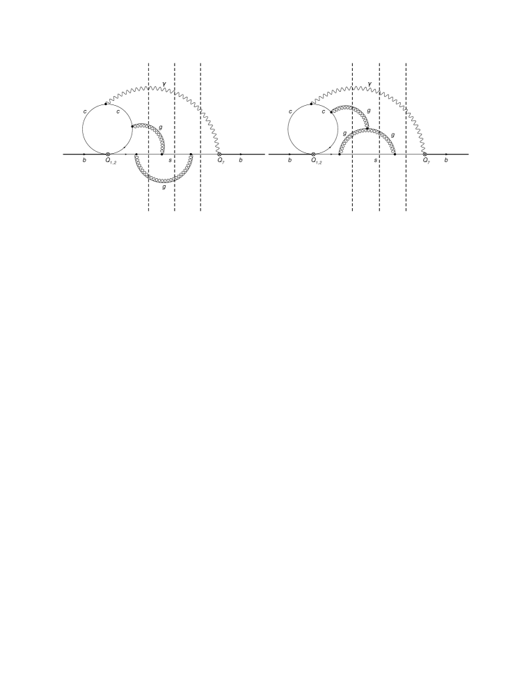
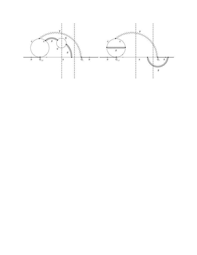
Figure 1: Sample diagrams for $\widetilde{G}^{(2)}_{(1,2)7}$ with some of the possible cuts indicated by the dashed lines.

For efficiency reasons, we work directly with cut diagrams and employ the technique first proposed in [44]. The idea of the method is to represent cut propagators as

$$-2\pi i\delta(p^{2}-m^{2})=\frac{1}{p^{2}-m^{2}+i\varepsilon}-\frac{1}{p^{2}-m^{2}-i\varepsilon}\;.$$ (2.1)

As long as we perform only algebraic transformations on the integrands, there is no difference between the first and second terms on the r.h.s. of the above equation, and it is sufficient to work with one of them only. This is particularly convenient for the integration-by-parts (IBP) method for reduction of integrals [45]. The only difference in such an approach between complete integrals and cut integrals is that a given integral vanishes if the cut propagator disappears due to cancellation of numerators with denominators. This fact reduces the number of occurring integrals in comparison to a computation without cuts.

In practice, the calculation follows the standard procedure. Diagrams are generated with DiaGen [46], the Dirac algebra is performed with FORM [47], and the resulting scalar integrals are reduced using IBP identities with IdSolver [46]. The main challenge of this calculation begins after these steps. The amplitudes for the interference contributions are expressed in terms of a number of master integrals, most of them containing massive internal $b$-quark lines and a non-trivial phase space integration in $D=4-2\epsilon$ spacetime dimensions, with up to four particles in the final state. A feeling for the size of the problem can be gained from Tab. 1.

	$n_{D}$	$n_{OS}$	$n_{\rm eff}$	$n_{\rm massless}$
two-particle cuts	292	92	143	9
three-particle cuts	267	54	110	11
four-particle cuts	292	17	37	7
total	851	163	290	27

Table 1: Number of diagrams $n_{{D}}$, number of massive on-shell master integrals $n_{{OS}}$, number of effectively computed massive master integrals $n_{\rm eff}$, and number of massless master integrals $n_{\rm massless}$. The last two columns are explained in the text.

Having a large number of massive cut integrals, it is advantageous to devise a strategy to treat them in a uniform manner. It is clear that purely massless cut integrals are easier to calculate than massive ones. Therefore, we aim at replacing a calculation of massive propagator integrals by a calculation of massless ones. This can be achieved by extending the integral definitions. We assume, namely, that the external momentum squared $p_{b}^{2}$ is a free parameter, and treat coefficients ${\mathcal{I}}_{i}$ in the $\epsilon$-expansion of the master integrals as functions of a single dimensionless variable $x=p_{b}^{2}/m_{b}^{2}$. IBP identities give us differential equations

$$\frac{d}{dx}{\mathcal{I}}_{i}(x)=\sum_{j}{\mathcal{J}}_{ij}(x){\mathcal{I}}_{j}(x)\;,$$ (2.2)

with ${\mathcal{J}}_{ij}(x)$ being certain rational functions of $x$. Boundary conditions for these equations in the vicinity of $x=0$ are given by asymptotic large-mass expansions, i.e. by power-log series in $x$. A few leading terms in the series for each ${\mathcal{I}}_{i}$ can be found by calculating products of massive tadpole integrals up to three loops and massless propagator ones up to four loops, as illustrated in Fig. 2. Next, higher-order terms can be determined from the differential equations themselves by substituting ${\mathcal{I}}_{i}$ in terms of power-log series in $x$. For our application it turns out that around 50 terms are sufficient to obtain the desired accuracy. This gives us high-precision boundary conditions at small but non-vanishing $x$ for solving the differential equations (2.2) numerically.

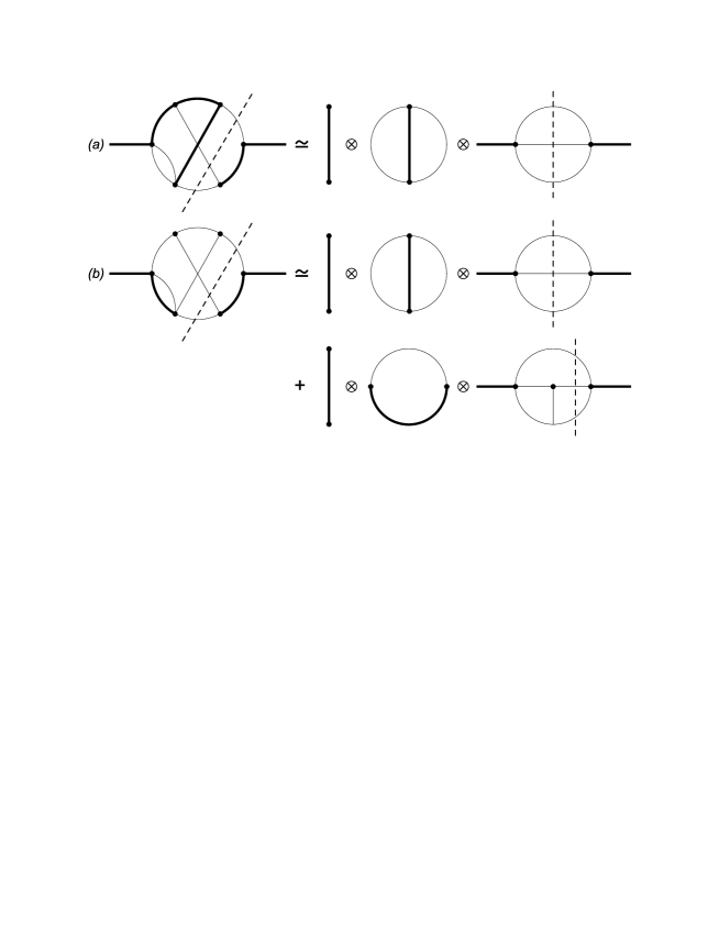
Figure 2: Diagrammatic representation of the asymptotic large mass expansion of two non-planar master integrals.Thick and thin lines represent massive and massless propagators, respectively, while dashed lines show the unitarity cuts.

On the way from the vicinity of $x=0$ to the physical point at $x=1$, one often encounters spurious singularities on the real axis. To bypass them, the differential equations are solved along ellipses in the complex $x$ plane. Several such ellipses are usually considered to test whether the numerical solution is stable.

Naively, one might think that as long as there are no infinities at $x=1$, the numerical solution could be continued up to that point. However, there is an essential singularity there, and the integrals behave as $(1-x)^{n}\ln^{m}(1-x)$, with $n,m>0$ being some positive powers. Due to such a behaviour, the numerical solution has poor convergence, as the algorithms assume locally polynomial behaviour of the considered functions. In order to overcome this problem, we perform another power-log expansion around $x=1$, and match it onto the numerical result. To determine the maximal power of the logarithms, we begin with observing that the highest poles in the cut diagrams could potentially be of order $1/\epsilon^{6}$, due to the presence of collinear and soft divergences. The coefficient of the leading singularity contains no  $\ln(1-x)$ because logarithms are generated by expanding expressions of the form $(1-x)^{a\epsilon}/\epsilon^{6}$ (with $a$ being some constant) in the framework of expansion by regions. Thus, finite parts of the master integral expansions may only contain $\ln^{6}(1-x)$. Higher powers may be needed due to the presence of spurious singularities, i.e. poles in the coefficients at the master integrals in the physical amplitude. In practice, we have used an ansatz with logarithm powers up to fifteen. Our numerical matching has shown that such high powers never occur in the considered problem, i.e. the respective expansion coefficients are consistent with zero to very high numerical precision. Using the matched series, we finally obtain the required values of the original master integrals at $x=1$. The solution procedure is schematically represented in Fig. 3a.

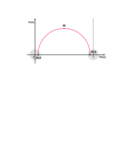
Figure 3: Left (a): Integration contour in the complex $x$ plane. The numerical integration (NI) is performed between the regions close to $x=0$ and $x=1$ that are accessible by power-log expansions (PLE).  Right (b): Diagrams that give the terms marked with $\kappa$ in Eq. (2.3).

Since the master integrals are considered for $x\neq 1$, their overall number $n_{\rm eff}$ is larger than it would be for $x=1$, i.e. $n_{\rm eff}>n_{OS}$. However, the massless integrals that are necessary to determine the boundary conditions near $x=0$ are not only simpler, but also their number $n_{\rm massless}$ is much smaller than $n_{OS}$, as seen in Tab. 1. All the massless integrals that we had to consider are depicted in Appendix A, in Fig. 7 and Tab. 3.

Using the above method, we have obtained the following bare NNLO results for the considered interferences in the Feynman-’t Hooft gauge:

$$\widetilde{G}_{17}^{(2)\rm bare} = -\frac{1}{6}\widetilde{G}_{27}^{(2)\rm bare}+\frac{80}{81\,\epsilon^{2}}+\frac{1592+54\pi^{2}}{243\,\epsilon}+42.0026519628,$$

$$\widetilde{G}_{27}^{(2)\rm bare} = -\frac{4}{3\,\epsilon^{3}}-\frac{30332+432\pi^{2}}{2187\,\epsilon^{2}}-\frac{67.66077706444119}{\epsilon}+44.5070537274$$ (2.3)

$$+ \kappa\,n_{l}\left(\frac{32}{729\,\epsilon}+0.6520676315\right)+n_{l}\left(\frac{352}{729\,\epsilon^{2}}+\frac{11624}{2187\,\epsilon}+\frac{228656}{6561}-\frac{188}{243}\pi^{2}\right)$$

$$+ n_{b}\left(\frac{352}{729\,\epsilon^{2}}+\frac{5.17409838118169}{\epsilon}+15.1790288135\right)+{\mathcal{O}}(\epsilon).$$

Here, $n_{l}$ and $n_{b}$ denote numbers of massless and massive ($m=m_{b}$) quark flavours, while $\kappa=1$ marks contributions from the diagrams in Fig. 3b describing interferences involving four-body $sq\bar{q}\gamma$ final states and no $c\bar{c}\gamma$ couplings. The terms proportional to $n_{l}$ and $n_{b}$ but not marked by $\kappa$ reproduce (after renormalization) the $m_{c}\to 0$ limits of what is already known for non-zero $m_{c}$ [30, 31, 32]. For compactness, all the results in this subsection are given for $\mu^{2}=e^{\gamma}m_{b}^{2}/(4\pi)$, where $\gamma$ is the Euler-Mascheroni constant.

Some of the numbers in Eq. (2.3) have been given in an exact form even though our calculation of the master integrals at $x=1$ is purely numerical. However, the accuracy is very high (to around 14 decimals), so identification of simple rationals is possible. Moreover, renormalization gives us relations to lower-order results where more terms are known in an exact manner (see below). For the $n_{l}$-term, after verifying numerical agreement with Refs. [30, 39], we have made use of the available exact expressions. Several other numbers in this subsection that have been retained in a decimal form can actually be related to quantities encountered in Ref. [43], as described in Appendix B.

Let us now list all the lower-order bare contributions that are needed for renormalization. For this purpose, it is convenient to express Eq. (1.8) in terms of $C_{i}$ rather than $C_{i}^{\rm eff}$, and denote the corresponding interference terms by $\hat{G}_{ij}^{(n)}$ rather than $\widetilde{G}_{ij}^{(n)}$. All the necessary $\hat{G}_{i7}^{(0)}$ and $\hat{G}_{i7}^{(1)\rm bare}$ read

$$\hat{G}_{77}^{(0)} = \frac{\Gamma(2-\epsilon)\,e^{\gamma\epsilon}}{\Gamma(2-2\epsilon)},$$

$$\hat{G}_{47}^{(0)} = \frac{4}{3}\hat{G}_{37}^{(0)}~{}=~{}-\frac{4}{9}\,\Gamma(1+\epsilon)\;e^{\gamma\epsilon}\;\hat{G}_{77}^{(0)},$$

$$\hat{G}_{67}^{(0)} = \frac{4}{3}\hat{G}_{57}^{(0)}~{}=~{}4\left(5-3\,\epsilon-\,\epsilon^{2}\right)\,\hat{G}_{47}^{(0)},$$

$$\hat{G}_{27}^{(1)\rm bare} = -6\,\hat{G}_{17}^{(1)\rm bare}~{}=~{}-\frac{92}{81\,\epsilon}-\frac{1978}{243}+\frac{777\pi^{2}-27185}{729}\,\epsilon+{\mathcal{O}}(\epsilon^{2}),$$

$$\hat{G}_{47}^{(1)\rm bare} = \frac{16}{3\,\epsilon^{2}}+\frac{3674}{243\,\epsilon}+43.76456245573869+94.9884724116\,\epsilon$$

$$+ \kappa\,n_{l}\left(-\frac{16}{243}+\frac{44\pi^{2}-612}{243}\,\epsilon\right)+n_{l}\left(\frac{16}{81\,\epsilon}-\frac{4}{243}+\frac{264\pi^{2}-2186}{729}\,\epsilon\right)$$

$$+ n_{b}\left(\frac{16}{81\,\epsilon}+0.04680853247986+0.3194493123\,\epsilon\right)+{\mathcal{O}}(\epsilon^{2}),$$

$$\hat{G}_{77}^{(1)\rm bare} = \frac{4}{3\,\epsilon}+\frac{124}{9}-\frac{16}{9}\pi^{2}+\left(\frac{212}{3}-\frac{58}{9}\pi^{2}-\frac{64}{3}\zeta_{3}\right)\epsilon+{\mathcal{O}}(\epsilon^{2}),$$

$$\hat{G}_{78}^{(1)\rm bare} = \frac{16}{9\,\epsilon}+\frac{280}{27}-\frac{16}{27}\pi^{2}+\left(\frac{382}{9}-\frac{16}{9}\pi^{2}-\frac{160}{9}\zeta_{3}\right)\epsilon+{\mathcal{O}}(\epsilon^{2}),$$

$$\hat{G}_{7(12)}^{(1)\rm bare} = -6\,\hat{G}_{7(11)}^{(1)\rm bare}~{}=~{}\frac{2096}{81}+\frac{39832}{243}\,\epsilon+{\mathcal{O}}(\epsilon^{2}).$$ (2.4)

The last line of the above equation describes contributions from the so-called evanescent operators that vanish in four spacetime dimensions

$$Q_{11} = (\bar{s}_{L}\gamma_{\mu_{1}}\gamma_{\mu_{2}}\gamma_{\mu_{3}}T^{a}c_{L})(\bar{c}_{L}\gamma^{\mu_{1}}\gamma^{\mu_{2}}\gamma^{\mu_{3}}T^{a}b_{L})-16Q_{1},$$

$$Q_{12} = (\bar{s}_{L}\gamma_{\mu_{1}}\gamma_{\mu_{2}}\gamma_{\mu_{3}}c_{L})(\bar{c}_{L}\gamma^{\mu_{1}}\gamma^{\mu_{2}}\gamma^{\mu_{3}}b_{L})-16Q_{2}.$$ (2.5)

In $\hat{G}_{(1,2)7}^{(1)\rm bare}$, the three-particle-cut contributions alone ($b\to s\gamma g$) read

$$\hat{G}_{27}^{(1)3P}=-6\,\hat{G}_{17}^{(1)3P}=-\frac{4}{27}-\frac{106}{81}\,\epsilon+{\mathcal{O}}(\epsilon^{2}).$$ (2.6)

In addition, several interferences need to be calculated with the $b$-quark propagators squared, to account for the renormalization of $m_{b}$. We find

$$\hat{G}_{27}^{(1)m} = -6\,\hat{G}_{17}^{(1)m}~{}=~{}-\frac{1}{3\,\epsilon^{2}}-\frac{21+4\pi^{2}}{81\,\epsilon}+\frac{1085}{81}-\frac{161}{972}\pi^{2}-\frac{40}{27}\zeta_{3}$$

$$+ \left(\frac{59071}{486}-\frac{1645}{2916}\pi^{2}-\frac{65}{81}\zeta_{3}-\frac{7}{81}\pi^{4}\right)\epsilon+{\mathcal{O}}(\epsilon^{2}),$$

$$\hat{G}_{47}^{(0)m} = \frac{4}{3\epsilon}+2+\frac{50-2\pi^{2}}{9}\,\epsilon+\frac{94-3\pi^{2}-32\zeta_{3}}{9}\,\epsilon^{2}+{\mathcal{O}}(\epsilon^{3}).$$ (2.7)

Our conventions for their global normalization will become clear through the way they enter the renormalized NNLO expression in Eq. (2.21) below.

Some of the diagrams with $Q_{4}$ insertions contain $b$-quark tadpoles that are the only source of $1/\epsilon^{2}$ terms in $\hat{G}_{47}^{(1)\rm bare}$, and $1/\epsilon$ terms in $\hat{G}_{47}^{(0)m}$. Such divergences are actually necessary to renormalize the $1/\epsilon^{3}$ poles in Eq. (2.3). These tadpole diagrams have been skipped in the NLO calculation of Ref. [43] because they give no contribution to the renormalized $\hat{G}_{47}^{(1)}$, i.e. they cancel out after renormalization of $m_{b}$.

Among all the bare interferences given in this section, not only the NNLO ones are entirely new, but also $\hat{G}_{7(12)}^{(1)\rm bare}$, $\hat{G}_{27}^{(1)m}$ and $\hat{G}_{47}^{(0)m}$. The remaining LO and NLO results are extensions of the known ones by another power of $\epsilon$, as necessary for the current calculation.

2.2 Renormalization

Our results in the previous subsection contain no loop corrections on external legs in the interfered amplitudes. Such corrections are taken into account below, with the help of on-shell renormalization constants for the $b$-quark, $s$-quark and gluon fields

$$Z_{b}^{\rm OS} = 1-\frac{4}{3}\,\widetilde{\alpha}_{\mathrm{s}}\,s^{\epsilon}\,e^{\gamma\epsilon}\,\Gamma(\epsilon)\,\frac{3-2\epsilon}{1-2\epsilon}+{\mathcal{O}}(\widetilde{\alpha}_{\mathrm{s}}^{2}),$$

$$Z_{s}^{\rm OS} = 1+{\mathcal{O}}(\widetilde{\alpha}_{\mathrm{s}}^{2}),$$

$$Z_{G}^{\rm OS} = 1-\frac{2}{3}\,n_{b}\,\widetilde{\alpha}_{\mathrm{s}}\,s^{\epsilon}\,e^{\gamma\epsilon}\,\Gamma(\epsilon)\,+{\mathcal{O}}(\widetilde{\alpha}_{\mathrm{s}}^{2}),$$ (2.8)

where $\widetilde{\alpha}_{\mathrm{s}}=\frac{\alpha_{\mathrm{s}}}{4\pi}=\frac{g_{s}^{2}}{16\pi^{2}}$ and $s=\frac{4\pi\mu^{2}}{m_{b}^{2}}e^{-\gamma}$. The QCD coupling $g_{s}$ and the Wilson coefficients $C_{i}$ are renormalized in the $\overline{\rm MS}$ scheme: $g_{s}^{\rm bare}=\bar{Z}_{g}g_{s}$, and $C_{i}^{\rm bare}=\sum_{j}C_{j}\bar{Z}_{ji}$. The corresponding ${\rm MS}$ renormalization constants can be taken over from the literature (see, e.g., Refs. [17, 19])

$$\begin{array}[]{rclrcl}Z_{g}&=&1+\frac{\widetilde{\alpha}_{\mathrm{s}}}{\epsilon}\left(-\frac{11}{2}+\frac{f}{3}\right)+{\mathcal{O}}(\widetilde{\alpha}_{\mathrm{s}}^{2}),{}{}{}{}&Z_{77}&=&1+\frac{16\,\widetilde{\alpha}_{\mathrm{s}}}{3\,\epsilon}+{\mathcal{O}}(\widetilde{\alpha}_{\mathrm{s}}^{2}),\\[5.69054pt] Z_{11}&=&1-\frac{2\,\widetilde{\alpha}_{\mathrm{s}}}{\epsilon}+{\mathcal{O}}(\widetilde{\alpha}_{\mathrm{s}}^{2}),&Z_{21}&=&\frac{6\,\widetilde{\alpha}_{\mathrm{s}}}{\epsilon}+{\mathcal{O}}(\widetilde{\alpha}_{\mathrm{s}}^{2}),\\[5.69054pt] Z_{12}&=&\frac{4\,\widetilde{\alpha}_{\mathrm{s}}}{3\,\epsilon}+{\mathcal{O}}(\widetilde{\alpha}_{\mathrm{s}}^{2}),&Z_{22}&=&1+{\mathcal{O}}(\widetilde{\alpha}_{\mathrm{s}}^{2}),\\[5.69054pt] Z_{13}&=&\widetilde{\alpha}_{\mathrm{s}}^{2}\left(\frac{10}{81\,\epsilon^{2}}-\frac{353}{243\,\epsilon}\right)+{\mathcal{O}}(\widetilde{\alpha}_{\mathrm{s}}^{3}),&Z_{23}&=&\widetilde{\alpha}_{\mathrm{s}}^{2}\left(-\frac{20}{27\,\epsilon^{2}}-\frac{104}{81\,\epsilon}\right)+{\mathcal{O}}(\widetilde{\alpha}_{\mathrm{s}}^{3}),\\[5.69054pt] Z_{14}&=&-\frac{1}{6}Z_{24}+\widetilde{\alpha}_{\mathrm{s}}^{2}\left(\frac{1}{2\epsilon^{2}}-\frac{11}{12\,\epsilon}\right),&Z_{24}&=&\frac{2\,\widetilde{\alpha}_{\mathrm{s}}}{3\,\epsilon}+\widetilde{\alpha}_{\mathrm{s}}^{2}\left(\frac{-188+12f}{27\,\epsilon^{2}}+\frac{338}{81\,\epsilon}\right)+{\mathcal{O}}(\widetilde{\alpha}_{\mathrm{s}}^{3}),\\[5.69054pt] Z_{15}&=&\widetilde{\alpha}_{\mathrm{s}}^{2}\left(-\frac{1}{81\,\epsilon^{2}}+\frac{67}{486\,\epsilon}\right)+{\mathcal{O}}(\widetilde{\alpha}_{\mathrm{s}}^{3}),&Z_{25}&=&\widetilde{\alpha}_{\mathrm{s}}^{2}\left(\frac{2}{27\,\epsilon^{2}}+\frac{14}{81\,\epsilon}\right)+{\mathcal{O}}(\widetilde{\alpha}_{\mathrm{s}}^{3}),\\[5.69054pt] Z_{16}&=&\widetilde{\alpha}_{\mathrm{s}}^{2}\left(-\frac{5}{216\,\epsilon^{2}}-\frac{35}{648\,\epsilon}\right)+{\mathcal{O}}(\widetilde{\alpha}_{\mathrm{s}}^{3}),&Z_{26}&=&\widetilde{\alpha}_{\mathrm{s}}^{2}\left(\frac{5}{36\,\epsilon^{2}}+\frac{35}{108\,\epsilon}\right)+{\mathcal{O}}(\widetilde{\alpha}_{\mathrm{s}}^{3}),\\[5.69054pt] Z_{17}&=&-\frac{1}{6}Z_{27}+\widetilde{\alpha}_{\mathrm{s}}^{2}\left(\frac{22}{81\,\epsilon^{2}}-\frac{332}{243\,\epsilon}\right),&Z_{27}&=&\frac{116\,\widetilde{\alpha}_{\mathrm{s}}}{81\,\epsilon}+\widetilde{\alpha}_{\mathrm{s}}^{2}\left(\frac{-3556+744f}{2187\,\epsilon^{2}}+\frac{13610-44f}{2187\,\epsilon}\right)+{\mathcal{O}}(\widetilde{\alpha}_{\mathrm{s}}^{3}),\\[5.69054pt] Z_{18}&=&\frac{167\,\widetilde{\alpha}_{\mathrm{s}}}{648\,\epsilon}+{\mathcal{O}}(\widetilde{\alpha}_{\mathrm{s}}^{2}),&Z_{28}&=&\frac{19\,\widetilde{\alpha}_{\mathrm{s}}}{27\,\epsilon}+{\mathcal{O}}(\widetilde{\alpha}_{\mathrm{s}}^{2}),\\[5.69054pt] Z_{1(11)}&=&\frac{5\,\widetilde{\alpha}_{\mathrm{s}}}{12\,\epsilon}+{\mathcal{O}}(\widetilde{\alpha}_{\mathrm{s}}^{2}),&Z_{2(11)}&=&\frac{\widetilde{\alpha}_{\mathrm{s}}}{\epsilon}+{\mathcal{O}}(\widetilde{\alpha}_{\mathrm{s}}^{2}),\\[5.69054pt] Z_{1(12)}&=&\frac{2\,\widetilde{\alpha}_{\mathrm{s}}}{9\,\epsilon}+{\mathcal{O}}(\widetilde{\alpha}_{\mathrm{s}}^{2}),&Z_{2(12)}&=&{\mathcal{O}}(\widetilde{\alpha}_{\mathrm{s}}^{2}),\\[5.69054pt] \end{array}$$ (2.19)

where  $f=n_{l}+n_{b}$  here, as we have skipped all the charm loops on the gluon lines. For the $b$-quark mass renormalization, we use the on-shell scheme everywhere ($Z_{m}^{\rm OS}=Z_{b}^{\rm OS}+{\mathcal{O}}(\widetilde{\alpha}_{\mathrm{s}}^{2})$), to get the overall $m_{b,\rm pole}^{5}$ in Eq. (1.8).

With all the necessary ingredients at hand, we can now write an explicit formula for the renormalized interference terms up to the NNLO ($i=1,2$)

$$\widetilde{\alpha}_{\mathrm{s}}\,\widetilde{G}_{i7}^{(1)}+\widetilde{\alpha}_{\mathrm{s}}^{2}\,\widetilde{G}_{i7}^{(2)} = Z_{b}^{\rm OS}\,Z_{m}^{\rm OS}\,\bar{Z}_{77}\left\{\widetilde{\alpha}_{\mathrm{s}}^{2}\,s^{3\epsilon}\,\widetilde{G}_{i7}^{(2)\rm bare}+(Z_{m}^{\rm OS}-1)\,s^{\epsilon}\left[\bar{Z}_{i4}\,\hat{G}_{47}^{(0)m}+\widetilde{\alpha}_{\mathrm{s}}\,s^{\epsilon}\,\hat{G}_{i7}^{(1)m}\right]\right.$$ (2.21)

$$+ \left.\widetilde{\alpha}_{\mathrm{s}}\,(Z_{G}^{\rm OS}-1)\,s^{2\epsilon}\,\hat{G}_{i7}^{(1)3P}+\bar{Z}_{i7}\,Z_{m}^{\rm OS}\left[\hat{G}_{77}^{(0)}+\widetilde{\alpha}_{\mathrm{s}}\,s^{\epsilon}\,\hat{G}_{77}^{(1)\rm bare}\right]+\widetilde{\alpha}_{\mathrm{s}}\,\bar{Z}_{i8}\,s^{\epsilon}\,\hat{G}_{78}^{(1)\rm bare}\right.$$

$$+ \left.\sum_{j=1,\ldots,6,11,12}\bar{Z}_{ij}\,s^{\epsilon}\left[\hat{G}_{j7}^{(0)}+\widetilde{\alpha}_{\mathrm{s}}\,s^{\epsilon}\,\bar{Z}_{g}^{2}\,\hat{G}_{j7}^{(1)\rm bare}\right]\right\}~{}+~{}{\mathcal{O}}(\widetilde{\alpha}_{\mathrm{s}}^{3}),$$

where $\hat{G}_{j7}^{(0)}=0$ for $j=1,2,11,12$. Once the above expression is expanded in $\widetilde{\alpha}_{\mathrm{s}}$, and ${\mathcal{O}}(\widetilde{\alpha}_{\mathrm{s}}^{3})$ terms are neglected, all the $1/\epsilon^{n}$ poles cancel out as they should. Our final renormalized results at $E_{0}=m_{c}=0$ read

$$\widetilde{G}_{27}^{(1)} = -6\,\widetilde{G}_{17}^{(1)}~{}=~{}-\frac{1702}{243}\;-\;\frac{416}{81}\ln\frac{\mu}{m_{b}},$$

$$\widetilde{G}_{17}^{(2)} = -\frac{1}{6}\widetilde{G}_{27}^{(2)}\;+\;\frac{136}{27}\ln^{2}\frac{\mu}{m_{b}}\;+\;\frac{94+8\pi^{2}}{9}\ln\frac{\mu}{m_{b}}\;+\;22.6049613485,$$

$$\widetilde{G}_{27}^{(2)} = \left(\frac{11792}{729}\;+\;\frac{800}{243}\,(n_{l}+n_{b})\right)\ln^{2}\frac{\mu}{m_{b}}\;+\;\left(1.0460332197\;+\;\frac{64}{729}\,\kappa\,n_{l}\right.$$ (2.22)

$$+ \left.\frac{2368}{243}\,n_{l}+9.6604967166\,n_{b}\right)\ln\frac{\mu}{m_{b}}\;-\;14.0663747289\;+\;0.1644478609\,\kappa\,n_{l}$$

$$+ \left(\frac{54170}{6561}\;+\;\frac{92}{729}\pi^{2}\right)\,n_{l}\;-\;1.8324081161\,n_{b}.$$

They are, of course, insensitive to conventions for the global $1+{\mathcal{O}}(\epsilon)$ normalization factor in Eqs. (2.3)–(2.7), so long as it is the same in all these equations. In particular, it does not matter that our $\hat{G}^{(0)}_{77}$ differs from the one in Ref. [25] by an overall factor of  $\Gamma(1+\epsilon)\,e^{\gamma\epsilon}$.

As already mentioned, the $n_{l}$ terms not marked by $\kappa$ in Eq. (2.22) agree with the previous calculations where both $m_{c}\neq 0$ and $m_{c}=0$ were considered. In the case of the $n_{b}$ terms, the current result extends the published fit (Eq. (3.3) of Ref. [32]) down to $m_{c}=0$. All the remaining terms are entirely new.

3 Impact of the NNLO corrections to $(Q_{7},Q_{1,2})$ interferences on the branching ratio

In the description of our phenomenological analysis, we shall strictly follow the notation of Ref. [34], where the relevant perturbative quantity

$$P(E_{0})~{}=~{}\sum_{i,j=1}^{8}C_{i}^{\rm eff}(\mu_{b})\;C_{j}^{\rm eff}(\mu_{b})\;K_{ij}(E_{0},\mu_{b}),$$ (3.1)

has been defined through

$$\frac{\Gamma[b\to X^{p}_{s}\gamma]_{E_{\gamma}>E_{0}}}{|V_{cb}/V_{ub}|^{2}\;\Gamma[b\to X^{p}_{u}e\bar{\nu}]}~{}=~{}\left|\frac{V^{*}_{ts}V_{tb}}{V_{cb}}\right|^{2}\frac{6\alpha_{\rm em}}{\pi}\;P(E_{0}).$$ (3.2)

The relation between $\widetilde{G}_{i7}^{(n)}$ for  $i=1,2$  and $K_{i7}=\widetilde{\alpha}_{\mathrm{s}}K_{i7}^{(1)}+\widetilde{\alpha}_{\mathrm{s}}^{2}K_{i7}^{(2)}+{\mathcal{O}}(\widetilde{\alpha}_{\mathrm{s}}^{3})$ is thus very simple

$$\widetilde{\alpha}_{\mathrm{s}}K_{i7}^{(1)}+\widetilde{\alpha}_{\mathrm{s}}^{2}K_{i7}^{(2)}+{\mathcal{O}}(\widetilde{\alpha}_{\mathrm{s}}^{3})~{}=~{}\frac{\widetilde{\alpha}_{\mathrm{s}}\,\widetilde{G}_{i7}^{(1)}+\widetilde{\alpha}_{\mathrm{s}}^{2}\,\widetilde{G}_{i7}^{(2)}+{\mathcal{O}}(\widetilde{\alpha}_{\mathrm{s}}^{3})}{1\;+\;\widetilde{\alpha}_{\mathrm{s}}(50-8\pi^{2})/3\;+\;{\mathcal{O}}(\widetilde{\alpha}_{\mathrm{s}}^{2})}\;,$$ (3.3)

where the denominator comes from the NLO correction to the semileptonic $b\to X^{p}_{u}e\bar{\nu}$ decay rate.

In the following, we shall write expressions for $K_{i7}^{(2)}$ that are valid for arbitrary $m_{c}$ and $E_{0}$ but incorporate information from our calculation in the previous section, where $E_{0}=m_{c}=0$ has been assumed. For this purpose, four functions

$$f_{\scriptscriptstyle NLO}(z,\delta) = {\rm Re}\,r_{2}^{(1)}(z)~{}+~{}2\phi^{(1)}_{27}(z,\delta),$$

$$f_{q}(z,\delta) = {\rm Re}\,r_{2}^{(2)}(z)~{}-~{}{\textstyle\frac{4}{3}}h^{(2)}_{27}(z,\delta),$$

$$f_{b}(z) \simeq -1.836+2.608\,z+0.8271\,z^{2}-2.441\,z\ln z,$$

$$f_{c}(z) \simeq 9.099+13.20\,z-19.68\,z^{2}+25.71\,z\ln z,$$ (3.4)

of $z=m_{c}^{2}/m_{b}^{2}$ and $\delta=1-2E_{0}/m_{b}$ are going to be useful. Explicit formulae for $r_{2}^{(1)}(z)$ and ${\rm Re}\,r_{2}^{(2)}(z)$ can be found in Eq. (3.1) of Ref. [43] and Eq. (26) of Ref. [30], respectively. For $h^{(2)}_{27}(z,\delta)$, we shall use a numerical fit from Eq. (13) of Ref. [39]. An analytical expression for $\phi^{(1)}_{27}(z,\delta)$  for  $4z<1-\delta$  (which is the phenomenologically relevant region) reads

$$\phi^{(1)}_{27}(z,\delta) = -\frac{2}{27}\delta(3-3\delta+\delta^{2})+\frac{4}{3}z\,\delta\,s_{\delta}\,L_{\delta}+\frac{12-8\pi^{2}}{9}z^{2}\delta+\frac{4}{3}z(1-2z)(s_{0}L_{0}-s_{\delta}L_{\delta})$$ (3.5)

$$+ \frac{2\pi^{2}-7}{9}z\delta(2-\delta)-\frac{8}{9}z(6z^{2}-4z+1)(L_{0}^{2}-L_{\delta}^{2})-\frac{8}{9}z\delta(2-\delta-4z)L_{\delta}^{2},$$

with  $s_{\delta}=\sqrt{(1-\delta)(1-\delta-4z)}$,  $s_{0}=\sqrt{1-4z}$,  $L_{\delta}=\ln\frac{\sqrt{1-\delta}+\sqrt{1-\delta-4z}}{2\sqrt{z}}$  and  $L_{0}=\ln\frac{1+\sqrt{1-4z}}{2\sqrt{z}}$.

In the $\delta=1$ case, $\phi^{(1)}_{27}$ and $h^{(2)}_{27}$ for $z<\frac{1}{4}$ are given by

$$\phi^{(1)}_{27}(z,1) = -\frac{2}{27}+\frac{12-8\pi^{2}}{9}z^{2}+\frac{4}{3}z(1-2z)s_{0}L_{0}+\frac{2\pi^{2}-7}{9}z-\frac{8}{9}z(6z^{2}-4z+1)L_{0}^{2}+\frac{4}{3}\pi^{2}z^{3},$$

$$h^{(2)}_{27}(z,1) \simeq \frac{41}{27}-\frac{2}{9}\pi^{2}-2.24\,z^{1/2}-7.04\,z+23.72\,z^{3/2}+(-9.86\,z+31.28\,z^{2})\ln z.$$ (3.6)

The functions $f_{b}(z)$ and $f_{c}(z)$ in Eq. (3.4) come from Eqs. (3.3) and (3.4) of Ref. [32], respectively. These numerical fits (in the range $z\in[0.017,0.155]$) describe contributions from three-loop $b\to s\gamma$ amplitudes with massive $b$-quark and $c$-quark loops on the gluon lines.

The ratio $z=m_{c}^{2}/m_{b}^{2}$ is defined in terms of the $\overline{\rm MS}$-renormalized charm quark mass at an arbitrary scale $\mu_{c}$. In practice, we shall use $\mu_{c}=2.0\,$GeV as a central value. As far as the renormalization scheme for $m_{b}$ is concerned, we assume the following relation to the on-shell scheme

$$\frac{m_{b,\rm pole}}{m_{b}}=1+\widetilde{\alpha}_{\mathrm{s}}x_{m}+{\mathcal{O}}(\widetilde{\alpha}_{\mathrm{s}}^{2}).$$ (3.7)

In the 1S and kinetic schemes, one finds $x_{m}={\textstyle\frac{8}{9}}\pi\alpha_{\Upsilon}$ and $x_{m}=\frac{64\mu_{\rm kin}}{9m_{b}}\left(1+\frac{3\mu_{\rm kin}}{8m_{b}}\right)$, respectively. In our numerical analysis, the kinetic scheme is going to be used.

Complete expressions for the NNLO quantities $K^{(2)}_{17}$ and $K^{(2)}_{27}$ can now be written as follows

$$K^{(2)}_{17}(z,\delta) = -\frac{1}{6}K^{(2)}_{27}(z,\delta)+A_{1}+F_{1}(z,\delta)+\left(\frac{94}{81}-\frac{3}{2}K^{(1)}_{27}-\frac{3}{4}K^{(1)}_{78}\right)L_{b}-\frac{34}{27}L_{b}^{2},$$

$$K^{(2)}_{27}(z,\delta) = A_{2}+F_{2}(z,\delta)-\frac{3}{2}\beta_{0}^{n_{l}=3}f_{q}(z,\delta)+f_{b}(z)+f_{c}(z)+\frac{4}{3}\phi^{(1)}_{27}(z,\delta)\ln z$$ (3.8)

$$+ \left[(8L_{c}-2x_{m})\,z\frac{d}{dz}\;+\;(1-\delta)x_{m}\frac{d}{d\delta}\right]f_{\scriptscriptstyle NLO}(z,\delta)+\frac{416}{81}x_{m}$$

$$+ \left(\frac{10}{3}K^{(1)}_{27}-\frac{2}{3}K^{(1)}_{47}-\frac{208}{81}K^{(1)}_{77}-\frac{35}{27}K^{(1)}_{78}-\frac{254}{81}\right)L_{b}-\frac{5948}{729}L_{b}^{2},$$

where  $\beta_{0}^{n_{l}=3}=9$, $L_{b}=\ln(\mu_{b}^{2}/m_{b}^{2})$  and  $L_{c}=\ln(\mu_{c}^{2}/m_{c}^{2})$,  while the relevant $K_{ij}^{(1)}$ are collected in Appendix C.

The expressions  $A_{i}+F_{i}(z,\delta)$  contain all the contributions that are not yet known for the measured value of $m_{c}$. They correspond to those parts of the considered interference terms that are obtained by: (i) setting $\mu_{b}=m_{b}$, $\mu_{c}=m_{c}$ and $x_{m}=0$, (ii) removing the BLM-extended contributions from quark loops on the gluon lines and from $b\to sq\bar{q}\gamma$ decays ($q=u,d,s$), except for those given in Fig. 3b.

We define the constants $A_{i}$ by requiring that $F_{i}(0,1)=0$. Then we evaluate $A_{i}$ from Eq. (2.22) by setting there $\mu=m_{b}$, $n_{b}=0$ and $\kappa n_{l}=3$. Next, a replacement $n_{l}\to n_{l}+\frac{3}{2}\beta_{0}^{n_{l}}=\frac{33}{2}$ is done in the remaining $n_{l}$-terms. Finally, Eq. (3.3) is used to find

$$A_{1}\simeq 22.605,\hskip 56.9055ptA_{2}\simeq 75.603.$$ (3.9)

These two numbers are the only outcome of our calculation in Section 2 that is going to be used in the phenomenological analysis below.

Apart from the condition $F_{i}(0,1)=0$, everything that is known at the moment about the functions $F_{i}(z,\delta)$ are their large-$z$ asymptotic forms. They can be derived from the results of Ref. [35]. Explicitly, we find

$$F_{1}(z,\delta) = \frac{70}{27}\ln^{2}z+\left(\frac{119}{27}-\frac{2}{9}\pi^{2}+\frac{3}{2}\phi^{(1)}_{78}(\delta)\right)\ln z-\frac{493}{2916}-\frac{5}{54}\pi^{2}+\frac{232}{27}\zeta_{3}+\frac{5}{8}\phi^{(1)}_{78}(\delta)$$

$$- A_{1}+{\mathcal{O}}\left(\frac{1}{z}\right),$$

$$F_{2}(z,\delta) = -\frac{4736}{729}\ln^{2}z+\left\{-\frac{165385}{2187}+\frac{1186}{729}\pi^{2}-\frac{2\pi}{9\sqrt{3}}+\frac{2}{3}Y_{1}+\frac{4}{3}\phi^{(1)}_{47}(\delta)+\frac{832}{81}\phi^{(1)}_{77}(\delta)\right.$$ (3.10)

$$+ \left.\frac{70}{27}\phi^{(1)}_{78}(\delta)\right\}\left(\ln z+1\right)-\frac{956435}{19683}-\frac{2662}{2187}\pi^{2}+\frac{20060}{243}\zeta_{3}-\frac{1624}{243}\phi^{(1)}_{77}(\delta)$$

$$- \frac{293}{162}\phi^{(1)}_{78}(\delta)-A_{2}+{\mathcal{O}}\left(\frac{1}{z}\right).$$

The constant $Y_{1}$ and the necessary $\phi^{(1)}_{ij}$ functions are given in Appendices B and C, respectively.

Let $\Delta{\mathcal{B}}_{s\gamma}$ denote the contribution from $F_{1,2}(z,\delta)$ to ${\mathcal{B}}_{s\gamma}$. Then the relative effect is given by

$$\frac{\Delta{\mathcal{B}_{s\gamma}}}{\mathcal{B}_{s\gamma}}~{}\simeq~{}U(z,\delta)~{}\equiv~{}\frac{\alpha_{\mathrm{s}}^{2}(\mu_{b})}{8\pi^{2}}\;\;\frac{C_{1}^{(0)}(\mu_{b})F_{1}(z,\delta)+\left(C_{2}^{(0)}(\mu_{b})-\frac{1}{6}C_{1}^{(0)}(\mu_{b})\right)F_{2}(z,\delta)}{C_{7}^{(0)\rm eff}(\mu_{b})}.$$ (3.11)

For $\mu_{b}=2.0\,$GeV, we have $\alpha_{s}(\mu_{b})\simeq 0.293$, $C_{1}^{(0)}(\mu_{b})\simeq-0.902$, $C_{2}^{(0)}(\mu_{b})\simeq 1.073$, and $C_{7}^{(0)\rm eff}(\mu_{b})\simeq-0.385$.

We shall estimate the contribution to ${\mathcal{B}}_{s\gamma}$ that comes from the unknown $U(z,\delta)$ by considering an interpolation model where $U(z,1)$ is given by the following linear combination

$$U_{\rm interp}(z,1)~{}=~{}x_{1}\,+\,x_{2}\,f_{q}(z,1)\,+\,\left(x_{3}\,+\,x_{4}\,z\frac{d}{dz}\right)f_{\scriptscriptstyle NLO}(z,1).$$ (3.12)

The numbers $x_{i}$ are fixed by the condition $U(0,1)=0$ as well as by the large-$z$ behaviour of $U(z,1)$ that follows from Eq. (3.10). This determines $x_{i}$ in a unique manner, namely $x_{i}\simeq(-0.0502,~{}0.0328,~{}0.0373,~{}0.0309)_{i}$. In Fig. 4, the function $U_{\rm interp}(z,1)$ is plotted with a solid line, while the dashed line shows $U_{\rm asymp}(z,1)$, i.e. asymptotic large-$z$ behaviour of the true $U(z,1)$. Note that $\sqrt{z}=m_{c}/m_{b}$ rather than $z$ is used on the horizontal axis. The vertical line corresponds to the measured value of this mass ratio. The plot involves some extra approximation in the region between $\sqrt{z}\simeq 0.4$ and $\sqrt{z}\simeq 0.8$ where we need to interpolate between the known small-$z$ and large-$z$ expansions of ${\rm Re\,}r_{2}^{(2)}(z)$ (see Fig. 1 of Ref. [34]).

In Refs. [34, 42] the uncertainty in ${\mathcal{B}}_{s\gamma}$ due to unknown $m_{c}$-dependence of the NNLO corrections has been estimated at the $\pm 3\%$ level. The size of the interpolated contribution in Fig. 4 implies that no reduction of this uncertainty is possible at the moment. One might wonder whether the uncertainty should not be enlarged. Our choice here is to leave it unchanged, for the following reasons:

Figure 4: The interpolating function defined in Eq. (3.12) (solid line) and asymptotic behaviour of the true function $U(z,1)$ for $m_{c}\gg m_{b}/2$ (dashed line). The vertical line corresponds to the measured value of $m_{c}/m_{b}$.

• Our choice of functions for the linear combination in Eq. (3.12) is dictated by the fact, that these very functions determine the dependence on $z$ of the known parts of $K^{(2)}_{17}$ and $K^{(2)}_{27}$. The known parts are either those related to renormalization of the Wilson coefficients and quark masses (in the terms proportional to $L_{b}$ and $L_{c}$) or the renormalization of $\alpha_{s}$ (the function $f_{q}$ parametrizes the considered correction in the BLM approximation). It often happens in perturbation theory that higher-order corrections are dominated by renormalization effects. If this is the case here, the true $U(z,1)$ should have a similar shape to $U_{\rm interp}(z,1)$.

• The growth of $U_{\rm interp}(z,1)$ for $m_{c}>m_{b}/2$ is perfectly understandable. In this region, logarithms of $z$ from Eq. (3.10) combine with $L_{b}$ from Eq. (3.8), and the asymptotic large-$m_{c}$ behaviour of $K^{(2)}_{(1,2)7}$ is determined by $\ln(\mu_{b}/m_{c})$ and $\ln(\mu_{c}/m_{c})$ only (see Eqs. (5.12) and (5.14) of Ref. [35]). Thus, the growth of the correction for large $z$ can be compensated by an appropriate choice of the renormalization scales, which means (not surprisingly) that the dangerous large logarithms can get resummed using renormalization group evolution of the Wilson coefficients, masses and $\alpha_{s}$.

• Our $\pm 3\%$ uncertainty is going to be combined in quadrature with the other ones, which means that it should be treated as a “theoretical $1\sigma$ error”. To gain higher confidence levels, it would need to be enlarged.

• In the considered interference terms $K_{17}$ and $K_{27}$, the dependence on $\delta$ is very weak in the whole range $\delta\in[0,1]$, both at the NLO and in the BLM approximation for the NNLO corrections. Specifically, changing $\delta$ from 1 ($E_{0}=0$) to 0.295 ($E_{0}=1.6\,$GeV) results in modifications of $f_{NLO}$ by $+0.2\%$ and $f_{q}$ by $+1.0\%$, respectively, for the measured value of $m_{c}$. The corresponding changes at $m_{c}=0$ amount to $-0.7\%$ and $-2.4\%$ only. Thus, our estimates made for $\delta=1$ are likely to be valid for arbitrary $\delta$.

In the phenomenological analysis below, we shall take $K^{(2)}_{17}$ and $K^{(2)}_{27}$ as they stand in Eq. (3.8), replace the unknown $F_{i}(z,\delta)$ by $F_{i}^{\rm interp}(z,1)$ interpolated analogously to Eq. (3.12)

$$F_{1}^{\rm interp}(z,1) = -23.75\,+\,\frac{35}{12}\,f_{q}(z,1)\,+\,\left(\frac{2129}{936}-\frac{9}{52}\pi^{2}\,-\,0.84\,z\frac{d}{dz}\right)f_{\scriptscriptstyle NLO}(z,1),$$

$$F_{2}^{\rm interp}(z,1) = -3.01\,-\,\frac{592}{81}\,f_{q}(z,1)\,+\,\left(-10.34\,-\,9.55\,z\frac{d}{dz}\right)f_{\scriptscriptstyle NLO}(z,1),$$ (3.13)

and include a $\pm 3\%$ uncertainty in the branching ratio due to such an approximation.

4 Evaluation of ${\mathcal{B}}_{s\gamma}$ in the SM

In the present section, we include all the other corrections to ${\mathcal{B}}_{s\gamma}$ that have been evaluated after the analysis in Refs. [34, 42]. Next, we update the SM prediction. To provide information on sizes of the subsequent corrections, the description is split into steps, and the corresponding modifications in the branching ratio central value are summarized in Tab. 2. The steps are as follows:

• We begin with performing the calculation precisely as it was described in Ref. [34] but only shifting from ${\mathcal{B}}(\bar{B}\to X_{s}\gamma)$ to ${\mathcal{B}}_{s\gamma}$, which amounts to CP-averaging the perturbative decay widths. No directly CP-violating non-perturbative corrections to ${\mathcal{B}}(\bar{B}\to X_{s}\gamma)$ were considered in Ref. [34]. It was not equivalent to neglecting them but rather to assuming that they have vanishing central values. A dedicated analysis in Ref. [48] leads to an estimate of  $0.4\pm 1.7\%$  for such effects.

  1	2	3	4	5	6	7	8	9	10	total
  $-0.6\%\!$	$+1.0\%\!$	$-0.2\%\!$	$+2.0\%\!$	$+1.0\%\!$	$+1.6\%\!$	$+2.1\%\!$	$-0.5\%\!$	$+0.2\%\!$	$-0.4\%\!$	$+6.4\%\!$

  
  

  Table 2: Shifts in the central value of ${\mathcal{B}}_{s\gamma}$ for $E_{0}=1.6\,$GeV at each step (see the text).

• The input parameters are updated as outlined in Appendix D. In particular, we use results of the very recent kinetic-scheme fit to the semileptonic $B$ decay data [49].

• Central values of the renormalization scales $(\mu_{c},\mu_{b})$ are shifted from $(1.5,2.5)\,$GeV to $(2,2)\,$GeV. Both scales are then varied in the ranges $[1.25,~{}5]\,$GeV to estimate the higher-order uncertainty. In the resulting range of ${\mathcal{B}}_{s\gamma}$, the value corresponding to the $(2,2)\,$GeV renormalization scales is more centrally located than the $(1.5,2.5)\,$GeV one, after performing all the updates 1-10 here. It is the main reason for shifting the default scales. The $(2,2)\,$GeV choice is also simpler (both scales are equal), and $\mu_{c}$ is exactly as in the fit from which we take $m_{c}(\mu_{c})$ (Appendix D). As far as $\mu_{b}$ is concerned, it should be of the same order as the energy transferred to the partonic system after the $b$-quark decay. For the leading $b\to s\gamma$ contribution from the photonic dipole operator $P_{7}$, this energy equals to $\frac{1}{2}m_{b}$ which gives $2.3\,$GeV when one substitutes $m_{b}=m_{b,kin}$ from Appendix D. Rounding 2.3 to either 2.5 or 2.0 for the default value is equally fine, given that the observed $\mu_{b}$-dependence of ${\mathcal{B}}_{s\gamma}$ is weak (see Fig. 6), and our range for $\mu_{b}$ is $[1.25,~{}5]\,$GeV.

• In the interpolation of $P_{2}^{(2)\rm rem}$ (see Ref. [34] for its definition), we shift to the so-called case (c) where the interpolated quantity at $m_{c}=0$ was given by the $(Q_{7},Q_{7})$ interference alone.

• The $m_{c}=0$ boundary for $P_{2}^{(2)\rm rem}$ is updated to include all the relevant interferences, especially the ones evaluated in Section 2. The thick solid (red) line in Fig. 5 shows the new $P_{2}^{(2)\rm rem}$ in such a case, while the remaining lines are as in Fig. 2 of Ref. [34] (somewhat shifted due to the parameter and scale modifications only).

  

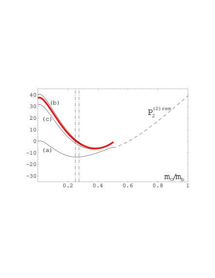
  Figure 5: Interpolation of $P_{2}^{(2)\rm rem}$ in $m_{c}$ as in Fig. 2 of Ref. [34] but with updated input parameters and with renormalization scales shifted to $(\mu_{c},\mu_{b})=(2,2)\,$GeV. In addition, the thick solid (red) line shows the case with the presently known boundary condition at $m_{c}=0$ imposed.

• At this point, we abandon the approach with $m_{c}$-interpolation applied to the whole non-BLM correction $P_{2}^{(2)\rm rem}$. As before, the penguin operators $Q_{3,\ldots,6}$ and the CKM-suppressed ones $Q^{u}_{1,2}$ are neglected at the NNLO level. The corrections $K^{(2)}_{17}$ and $K^{(2)}_{27}$ are treated as summarized at the end of the previous section. For $K^{(2)}_{78}$, the complete results from Refs. [36, 37] are included. $K^{(2)}_{77}$ is made complete by taking into account its exact $m_{c}$-dependence [29, 50], in addition to the previously included terms. For the NNLO interferences among $Q_{1}$, $Q_{2}$ and $Q_{8}$, only the two-body final state contributions are present at this step. They are infrared-finite by themselves, and given by products of the well-known NLO amplitudes $r_{i}^{(1)}$ (see Eq. (3.1) of Ref. [43]) whose imaginary parts matter here, too.

• Three- and four-body final state contributions to the NNLO interferences among $Q_{1}$, $Q_{2}$ and $Q_{8}$ are included in the BLM approximation, using the results of Refs. [31, 38, 39]. Non-BLM corrections to these interferences remain neglected. The corresponding uncertainty is going to be absorbed below into the overall $\pm 3\%$ perturbative one.

• Four-loop $Q_{1,\ldots,6}\to Q_{8}$ anomalous dimensions from Ref. [19] are included in the renormalization group equations.

• The LO and NLO contributions from four body final states are included [23, 24]. They are not yet formally complete, but the only neglected terms are the NLO ones that undergo double (quadratic) suppression either by the small Wilson coefficients $C_{3,\ldots,6}$ or by the small CKM element ratio $\left|V_{us}^{*}V_{ub}\right|/\left|V_{ts}^{*}V_{tb}\right|$. The uncertainty that results from neglecting such terms is below a permille in ${\mathcal{B}}_{s\gamma}$. As far as the CKM-suppressed two-body and three-body contributions are concerned, the two-body NLO one has already been taken into account in Ref. [34]. The remaining NLO and NNLO ones (also those with double CKM suppression) are included at the present step. Their contribution to ${\mathcal{B}}_{s\gamma}$ is below a permille. However, the branching ratio ${\mathcal{B}}_{d\gamma}$ [51] receives around 2% enhancement from them.

• We update our treatment of non-perturbative corrections. The ${\mathcal{O}}\left(\alpha_{\mathrm{s}}\Lambda^{2}/m_{b}^{2}\right)$ correction to the $(Q_{7},Q_{7})$ interference from Ref. [40] replaces the previous approximate expression from Ref. [52]. Moreover, we include a similar correction [41, 53] to the charmless semileptonic rate that is used for normalization in $[P(E_{0})+N(E_{0})]$ (see Eqs. (D.13) and (D.15) in Appendix D). In consequence, the previous (tiny) effect in $N(E_{0})$ gets reduced by a factor of around 4. Finally, our treatment of non-perturbative effects in interferences other than $(Q_{7},Q_{7})$ gets modified according to Ref. [14]. A vanishing contribution to the branching ratio central value from such corrections is assumed, except for the leading ${\mathcal{O}}\left(\lambda_{2}/m_{c}^{2}\right)$ one [54] where $m_{c}$ is fixed to $1.131\,$GeV. At the same time, a $\;\pm 5\%$ non-perturbative uncertainty in the branching ratio is assumed, as obtained in Sec. 7.4 of Ref. [14] by adding the relevant three uncertainties in a linear manner.

$\mu_{c}$                                                                        $\mu_{b}$
                                                                           $\mu_{0}$

Figure 6: Renormalization scale dependence of ${\cal B}_{s\gamma}$ in units $10^{-4}$ at the LO (dotted lines), NLO (dashed lines) and NNLO (solid lines). The upper-left, upper-right and lower plots describe the dependence on $\mu_{c}$, $\mu_{b}$ and $\mu_{0}$ [GeV], respectively. When one of the scales is varied, the remaining ones are set to their default values.

Our final result reads

$${\mathcal{B}}^{\rm SM}_{s\gamma}=(3.36\pm 0.23)\times 10^{-4}$$ (4.1)

for  $E_{0}=1.6\,$GeV, where four types of uncertainties have been combined in quadrature:$\pm 5\%$ non-perturbative (step 10 above), $\pm 3\%$ from our interpolation of $F_{1,2}(z,\delta)$ (Section 3), $\pm 2.0\%$ parametric (Appendix D), as well as $\pm 3\%$ from higher-order perturbative effects.

The latter uncertainty is assumed to account for approximations made at the NLO and NNLO levels, too. In the NLO case, it refers to the doubly suppressed terms mentioned in step 9 above. In the NNLO case, it refers to neglecting the penguin operators at this level, and using the BLM approximation in step 7 above. If we relied just on the renormalization-scale dependence in Fig. 6 (with $1.25\,{\rm GeV}<\mu_{c},\mu_{b}<5\,$GeV), we could reduce this uncertainty to around $\pm 2.4\%$. However, apart from the scale-dependence, one needs to study how the perturbation series behaves, which is hard to judge before learning the actual contributions from $F_{1,2}(z,\delta)$. Thus, we leave the higher-order uncertainty unchanged with respect to Refs. [34, 42]. Our treatment of the electroweak corrections [55] remains unchanged, too.

The central value in Eq. (4.1) is about 6.4% higher than the previous estimate of $3.15\times 10^{-4}$ in Refs. [34, 42]. Around half of this effect comes from improving the $m_{c}$-interpolation. As seen in Fig. 5, the currently known $m_{c}=0$ boundary for the thick line is close to the edge of the previously assumed range between the curves (a) and (b). It is consistent with the fact that the corrections in steps 4 and 5 sum up to 3% being the previous “$1\sigma$” interpolation uncertainty. The $m_{c}=0$ boundary has been the main worry in the past because estimating the range for its location was based on quite arbitrary assumptions. It is precisely the reason why no update of the SM prediction seemed to make sense until now, given moderate sizes of the other new corrections.

5 Conclusions

We evaluated ${\mathcal{O}}(\alpha_{s}^{2})$ contributions to the perturbative $\Gamma(b\to X_{s}\gamma)$ decay rate that originate from the $(Q_{7},Q_{1,2})$ interference for $m_{c}=E_{0}=0$. The calculation involved 163 four-loop massive on-shell propagator master integrals with unitarity cuts. Our updated prediction for the CP- and isospin-averaged branching ratio in the SM reads  ${\mathcal{B}}^{\rm SM}_{s\gamma}=(3.36\pm 0.23)\times 10^{-4}$. It includes all the perturbative and non-perturbative contributions that have been calculated to date. It agrees very well with the current experimental world average ${\mathcal{B}}^{\rm exp}_{s\gamma}=(3.43\pm 0.21\pm 0.07)\times 10^{-4}$. An extension of our analysis to the case of ${\mathcal{B}}_{d\gamma}$ and an update of bounds on the Two Higgs Doublet Model is going to be presented in a parallel article [51].

Appendix A:   Massless master integrals

4L4C1	4L4C2	4L4C3	4L4C4
4L4C5	4L4C6	4L4C7	4L4C8

Figure 7: The massless four-particle-cut diagrams calculated in the course of this work.

In the course of this work, it has been necessary to compute a number of massless scalar integrals with various unitarity cuts. All of them are depicted in Fig. 7 and Tab. 3. They occur after applying the large mass expansion for $p_{b}^{2}\ll m_{b}^{2}$, as well as in the decay rate calculation itself. Apart from the four-loop diagrams with four-particle cuts, and the four-loop diagrams 4L3C1, 4L3C2 and 4L3C3 with three-particle cuts, values of all our master integrals can either be found in the literature [56, 57, 58, 59, 60] or obtained using standard techniques described, for instance, in Ref. [64]. Let us note that the results for all the massless propagator four-loop master integrals in Refs. [65, 66] are not sufficient here because they correspond to sums over all the possible cuts, while certain cuts need to be discarded in our case.

2PCuts		3PCuts
1L2C1
2L2C1		2L3C1
3L2C1		3L3C1
4L2C1	4L2C2	4L3C1	4L3C2	4L3C3
4L2C3	4L2C4	4L3C4	4L3C5	4L3C6
4L2C5	4L2C6	4L3C7	4L3C8	4L3C9

Table 3: The massless two- and three-particle-cut diagrams used in the course of this work.

In the following, we explain our computation of the four-particle-cut master integrals in dimensional regularization with $D=4-2\epsilon$. The total momentum is $q=p_{1}+p_{2}+p_{3}+p_{4}$, and we have $p_{i}^{2}=0$ for $i=1,\ldots,4$. Moreover, all the internal lines are massless. The momenta are in Minkowski space, and we tacitly assume that all the propagators below contain an infinitesimal $+i\eta$ with $\eta>0$. We also define the invariants

$$s_{ijk\ldots}\equiv(p_{i}+p_{j}+p_{k}+\ldots)^{2}\;.$$ (A.1)

We therefore have $s_{12}+s_{13}+s_{14}+s_{23}+s_{24}+s_{34}=q^{2}$ as a constraint from overall momentum conservation.

Our convention for the loop measure is

$$\int\!\left[dk\right]\equiv\int\!\!\frac{d^{D}k}{i\left(2\pi\right)^{D}}\!\;,$$ (A.2)

and we define the prefactor

$$S_{\Gamma}\equiv\frac{1}{\left(4\pi\right)^{D/2}\Gamma(1-\epsilon)}\;.$$ (A.3)

Note that our definition of $S_{\Gamma}$ is different from the one in Eq. (4.13) of Ref. [57].

As far as integration over the four-particle massless phase space in $D=4-2\epsilon$ dimensions is concerned, we closely follow Ref. [57]. The phase space measure reads

$$dPS_{4}=\frac{d^{D-1}p_{1}}{(2\pi)^{D-1}\,2E_{1}}\ldots\frac{d^{D-1}p_{4}}{(2\pi)^{D-1}\,2E_{4}}\,(2\pi)^{D}\,\delta^{(D)}(q-p_{1}-p_{2}-p_{3}-p_{4})\,.$$ (A.4)

It can be rewritten in terms of invariants and angular variables according to

$$dPS_{4} = (2\pi)^{4-3D}\left(q^{2}\right)^{1-\frac{D}{2}}2^{1-\frac{D}{2}}\left(-\Delta_{4}\right)^{\frac{D-5}{2}}\theta(-\Delta_{4})\,d\Omega_{D-1}\,d\Omega_{D-2}\,d\Omega_{D-3}$$ (A.5)

$$\times\delta(q^{2}-s_{12}-s_{13}-s_{14}-s_{23}-s_{24}-s_{34})\,ds_{12}\,ds_{13}\,ds_{14}\,ds_{23}\,ds_{24}\,ds_{34}\;,$$

with the Gram determinant

$$\Delta_{4}=\lambda(s_{12}s_{34},s_{13}s_{24},s_{14}s_{23})\,,\qquad\lambda(x,y,z)=x^{2}+y^{2}+z^{2}-2xy-2xz-2yz\;.$$ (A.6)

It turns out that integration over angular variables is trivial in all the cases we encounter here, and we can use

$$\int\!\!d\Omega_{D}=\frac{2\pi^{D/2}}{\Gamma(D/2)}\;.$$ (A.7)

Performing the angular integration, and furthermore applying the steps explained in Ref. [57] to factorize the phase space measure, we arrive at

$$dPS_{4} = \frac{2\pi\left(q^{2}\right)^{2-3\epsilon}}{(4\pi)^{\frac{3D}{2}}(1-2\epsilon)\Gamma(1-\epsilon)\Gamma^{2}(\frac{1}{2}-\epsilon)}\,dt\,dv\,d\chi\,dz_{1}\,dy_{134}\,dy_{1234}\,\delta(1-y_{1234})$$

$$t^{-\epsilon}\,(1-t)^{-\epsilon}\,v^{-\epsilon}\,(1-v)^{-\epsilon}\,\chi^{-\frac{1}{2}-\epsilon}\,(1-\chi)^{-\frac{1}{2}-\epsilon}\,z_{1}^{-\epsilon}\,(1-z_{1})^{1-2\epsilon}\,y_{134}^{1-2\epsilon}\,(1-y_{134})^{1-2\epsilon}.$$

All the integration variables $t$, $v$, $\chi$, $z_{1}$, $y_{134}$, and $y_{1234}$ run from $0\ldots 1$ and originate from

$$s_{ijk\ldots} =q^{2}\,y_{ijk\ldots}\;, y_{13} =(y_{13,\,b}-y_{13,\,a})\chi+y_{13,\,a}\;,$$

$$y_{12} =\bar{y}_{134}\,\bar{z}_{1}\,\bar{t}\;, y_{13,\,b/a} =B\pm\sqrt{B^{2}-C}\;,$$

$$y_{23} =\bar{y}_{134}\,z_{1}\;, B =y_{134}\left(\bar{t}\,\bar{v}+v\,t\,z_{1}\right)\;,$$

$$y_{14} =y_{134}\,\bar{z}_{1}\,v\;, C =y_{134}^{2}\left(\bar{t}\,\bar{v}-v\,t\,z_{1}\right)^{2}\;,$$

$$y_{24} =\bar{y}_{134}\,\bar{z}_{1}\,t\;, \sqrt{B^{2}-C} =2\,y_{134}\,\sqrt{t}\,\sqrt{\bar{t}\,}\,\sqrt{v}\,\sqrt{\bar{v}}\,\sqrt{z_{1}}\;,$$

$$y_{124} =\bar{z}_{1}\left(1-y_{134}\bar{v}\right)\;, y_{13,\,b}-y_{13,\,a} =2\sqrt{B^{2}-C}\;,$$ (A.9)

where $\bar{t}=1-t$, and analogously for all the other variables. The substitutions (A.9) should be done in the integrands, too.

A.1  Results for the four-particle-cut master integrals

We are now in position to present results for the four-particle-cut diagrams depicted in Fig. 7. Normalization factors are extracted according to

$$I_{4L4Ci}=2\pi\,e^{i\pi\epsilon}\,S_{\Gamma}^{4}\left(q^{2}\right)^{a_{i}-4\epsilon}\,\widetilde{I}_{4L4Ci}\;,$$ (A.10)

where the $a_{i}$ follow from dimensional considerations. One finds $a_{i}=(2,2,1,-1,0,-1,-1,0)_{i}$ for $i=1,\ldots,8$.

We start with $I_{4L4C1}$,

$$I_{4L4C1} = \int\!\!dPS_{4}\!\int\!\left[dk\right]\,\frac{1}{k^{2}\,(k+p_{1}+p_{2})^{2}}$$ (A.11)

$$= \frac{e^{i\pi\epsilon}\,\Gamma(\epsilon)\Gamma^{2}(1-\epsilon)}{\left(4\pi\right)^{D/2}\Gamma(2-2\epsilon)}\,\left(q^{2}\right)^{-\epsilon}\!\int\!\!dPS_{4}\;y_{12}^{-\epsilon}\;,$$

which yields

$$\widetilde{I}_{4L4C1} = \frac{\Gamma(\epsilon)\Gamma^{9}(1-\epsilon)\Gamma(1-2\epsilon)\Gamma(2-3\epsilon)}{\Gamma^{2}(2-2\epsilon)\Gamma(3-4\epsilon)\Gamma(4-5\epsilon)}\;.$$ (A.12)

The next integral to consider is $I_{4L4C2}$,

$$I_{4L4C2} = \int\!\!dPS_{4}\!\int\!\left[dk\right]\,\frac{1}{k^{2}\,(k+p_{1}+p_{2}+p_{4})^{2}}$$ (A.13)

$$= \frac{e^{i\pi\epsilon}\,\Gamma(\epsilon)\Gamma^{2}(1-\epsilon)}{\left(4\pi\right)^{D/2}\Gamma(2-2\epsilon)}\,\left(q^{2}\right)^{-\epsilon}\!\int\!\!dPS_{4}\;y_{134}^{-\epsilon}\;,$$

and we get

$$\widetilde{I}_{4L4C2} = \frac{\Gamma(\epsilon)\Gamma^{10}(1-\epsilon)\Gamma(2-3\epsilon)}{\Gamma^{2}(2-2\epsilon)\Gamma(3-3\epsilon)\Gamma(4-5\epsilon)}\;.$$ (A.14)

We proceed with $I_{4L4C3}$,

$$I_{4L4C3} = \int\!\!dPS_{4}\!\int\!\left[dk\right]\,\frac{1}{k^{2}\,(k+p_{1}+p_{3}+p_{4})^{2}\,(p_{1}+p_{2}+p_{4})^{2}}$$ (A.15)

$$= \frac{e^{i\pi\epsilon}\,\Gamma(\epsilon)\Gamma^{2}(1-\epsilon)}{\left(4\pi\right)^{D/2}\Gamma(2-2\epsilon)}\,\left(q^{2}\right)^{-1-\epsilon}\!\int\!\!dPS_{4}\;y_{134}^{-\epsilon}\,y_{124}^{-1}\;,$$

and arrive at

$$\widetilde{I}_{4L4C3} = \frac{\Gamma(\epsilon)\Gamma^{10}(1-\epsilon)\Gamma(1-2\epsilon)}{\Gamma^{3}(2-2\epsilon)\Gamma(4-5\epsilon)}\;\,\!_{3}F_{2}(1,1-\epsilon,2-3\epsilon\,;\,2-2\epsilon,4-5\epsilon\,;\,1).$$ (A.16)

The expansion of $\widetilde{I}_{4L4C3}$ in $\epsilon$ is conveniently done with the package HypExp [68, 69],

$$\widetilde{I}_{4L4C3} = \frac{1}{4\epsilon}+\left(\frac{37}{8}-\frac{\pi^{2}}{12}\right)+\left(\frac{809}{16}-\frac{35\pi^{2}}{24}-5\zeta_{3}\right)\epsilon+\left(\frac{13677}{32}-\frac{253\pi^{2}}{16}-\frac{29\pi^{4}}{144}-71\zeta_{3}\right)\epsilon^{2}$$ (A.17)

$$+\left(\frac{198241}{64}-\frac{12995\pi^{2}}{96}-\frac{3521\pi^{4}}{1440}-\frac{1287}{2}\zeta_{3}+\frac{67}{6}\pi^{2}\zeta_{3}-\frac{315}{2}\zeta_{5}\right)\epsilon^{3}+\left(\frac{2597477}{128}\right.$$

$$\left.-\frac{192175\pi^{2}}{192}-\frac{17519\pi^{4}}{960}-\frac{1481\pi^{6}}{6048}-\frac{19139}{4}\zeta_{3}+\frac{925}{6}\pi^{2}\zeta_{3}+170\zeta_{3}^{2}-2049\zeta_{5}\right)\epsilon^{4}$$

$$+\,{\mathcal{O}}(\epsilon^{5})\;.$$

We now move to $I_{4L4C4}$,

$$I_{4L4C4} = \int\!\!dPS_{4}\!\int\!\left[dk\right]\,\frac{1}{k^{2}\,(k+p_{1}+p_{3}+p_{4})^{2}\,(p_{1}+p_{3})^{2}\,(p_{1}+p_{2}+p_{4})^{2}\,(p_{1}+p_{2})^{2}}$$ (A.18)

$$= \frac{e^{i\pi\epsilon}\,\Gamma(\epsilon)\Gamma^{2}(1-\epsilon)}{\left(4\pi\right)^{D/2}\Gamma(2-2\epsilon)}\,\left(q^{2}\right)^{-3-\epsilon}\!\int\!\!dPS_{4}\;y_{134}^{-\epsilon}\,y_{124}^{-1}\,y_{13}^{-1}\,y_{12}^{-1}\;,$$

which does not reveal a closed form since we cannot avoid $y_{13}$ in the integrand. We therefore compute it from the following two-fold Mellin-Barnes representation [61, 62, 63, 64, 67]

$$\widetilde{I}_{4L4C4} = \frac{\Gamma(\epsilon)\Gamma^{6}(1-\epsilon)\Gamma(-\epsilon)\Gamma(1-3\epsilon)}{\Gamma(-2\epsilon)\Gamma^{2}(2-2\epsilon)}\,\int\limits_{\hskip 15.0pt{}_{c_{1}-i\,\infty}}^{\hskip 15.0pt{}^{c_{1}+i\,\infty}}\frac{dz_{1}}{2\pi i}\int\limits_{\hskip 15.0pt{}_{c_{2}-i\,\infty}}^{\hskip 15.0pt{}^{c_{2}+i\,\infty}}\frac{dz_{2}}{2\pi i}\,\Gamma(z_{1}+z_{2}-\epsilon)\Gamma(-\epsilon-z_{1}-z_{2})\Gamma(z_{1})$$ (A.19)

$$\times\frac{\Gamma(1-z_{1})\Gamma(1-2\epsilon-z_{1})}{\Gamma(2-5\epsilon-z_{1})}\,\frac{\Gamma(-z_{2})\Gamma(1+z_{2})\Gamma(-1-\epsilon-z_{2})\Gamma(1-\epsilon+z_{2})}{\Gamma(1-3\epsilon+z_{2})\Gamma(-\epsilon-z_{2})}\,.$$

The integration contours in the complex plane can be chosen as straight lines parallel to the imaginary axis. The integral is then regulated [67] for $c_{1}=1/2$, $c_{2}=-1/4$, and $\epsilon=-7/4$. We perform an analytic continuation to $\epsilon=0$ with the package MB.m [67], which is also used for numerical cross checks. The expansion of $\widetilde{I}_{4L4C4}$ in $\epsilon$ reads

$$\widetilde{I}_{4L4C4} = \frac{1}{4\epsilon^{5}}+\frac{1}{\epsilon^{4}}+\left(3-\frac{13\pi^{2}}{24}\right)\frac{1}{\epsilon^{3}}+\left(8-\frac{13\pi^{2}}{6}-\frac{33}{2}\zeta_{3}\right)\frac{1}{\epsilon^{2}}+\left(20-\frac{13\pi^{2}}{2}-\frac{397\pi^{4}}{1440}\right.$$ (A.20)

$$-66\zeta_{3}\bigg{)}\frac{1}{\epsilon}+\left(48-\frac{52\pi^{2}}{3}-\frac{397\pi^{4}}{360}-198\zeta_{3}+\frac{131}{4}\pi^{2}\zeta_{3}-\frac{687}{2}\zeta_{5}\right)$$

$$+\left(112-\frac{130\pi^{2}}{3}-\frac{397\pi^{4}}{120}-\frac{24539\pi^{6}}{60480}-528\zeta_{3}+131\pi^{2}\zeta_{3}+\frac{897}{2}\zeta_{3}^{2}-1374\zeta_{5}\right)\epsilon$$

$$+\,{\mathcal{O}}(\epsilon^{2})\;.$$

The next integral, $I_{4L4C5}$, with

$$I_{4L4C5} = \int\!\!dPS_{4}\!\int\!\left[dk\right]\,\frac{1}{k^{2}\,(k+p_{4})^{2}\,(k+p_{1}+p_{2}+p_{4})^{2}\,(p_{2}+p_{3})^{2}}$$

$$= \frac{e^{i\pi\epsilon}\,\Gamma(1+\epsilon)\Gamma(-\epsilon)\Gamma(1-\epsilon)}{\left(4\pi\right)^{D/2}\Gamma(1-2\epsilon)}\!\left(q^{2}\right)^{-2-\epsilon}\!\!\int\!\!dPS_{4}\!\int\limits_{0}^{1}\!dx\;\frac{1}{\left[y_{12}+x\,y_{14}+x\,y_{24}\right]^{1+\epsilon}y_{23}},$$

can again be expressed to all orders in $\epsilon$. One first integrates over $x$, and finally finds

$$\widetilde{I}_{4L4C5} = -\,\frac{\Gamma(\epsilon)\Gamma^{6}(1-\epsilon)\Gamma^{3}(-\epsilon)}{\Gamma(2-5\epsilon)\Gamma(2-2\epsilon)}\left[\frac{\Gamma(1-\epsilon)}{\Gamma(2-2\epsilon)}\,\,\!_{3}F_{2}(1,1-\epsilon,1-2\epsilon\,;\,1+\epsilon,2-2\epsilon\,;\,1)\right.$$ (A.22)

$$\hskip 55.0pt\left.-\,\frac{\Gamma(1-3\epsilon)}{(1-3\epsilon)\Gamma(1-4\epsilon)}\,\,\!_{3}F_{2}(1,1-\epsilon,1-3\epsilon\,;\,1+\epsilon,2-3\epsilon\,;\,1)\right]\;.$$

The expansion of $\widetilde{I}_{4L4C5}$ in $\epsilon$ reads

$$\widetilde{I}_{4L4C5} = \frac{2\zeta_{3}}{\epsilon^{2}}+\left(14\zeta_{3}+\frac{31\pi^{4}}{180}\right)\frac{1}{\epsilon}+\left(78\zeta_{3}+\frac{217\pi^{4}}{180}-\frac{20}{3}\pi^{2}\zeta_{3}+114\zeta_{5}\right)$$ (A.23)

$$+\left(406\zeta_{3}+\frac{403\pi^{4}}{60}-\frac{140}{3}\pi^{2}\zeta_{3}+798\zeta_{5}+\frac{799\pi^{6}}{7560}-125\zeta_{3}^{2}\right)\epsilon+\,{\mathcal{O}}(\epsilon^{2})\;.$$

Also the next integral, $I_{4L4C6}$, with

$$I_{4L4C6} = \int\!\!dPS_{4}\!\int\!\left[dk\right]\,\frac{1}{k^{2}\,(k-p_{2})^{2}\,(k+p_{4})^{2}\,(k+p_{1}+p_{4})^{2}\,(p_{1}+p_{2})^{2}}$$

$$= \frac{e^{i\pi\epsilon}\,\Gamma(2+\epsilon)\Gamma^{2}(-\epsilon)}{\left(4\pi\right)^{D/2}\Gamma(-2\epsilon)}\!\left(q^{2}\right)^{-3-\epsilon}\!\!\int\!\!dPS_{4}\!\int\limits_{0}^{1}\!dx\!\int\limits_{0}^{1}\!dy\;\frac{1}{\left[x\,y_{24}+y\,y_{14}+xy\,y_{12}\right]^{2+\epsilon}y_{12}},$$

reveals a closed form which, however, turns out to be more complicated. One first integrates over $x$ and $y$, and finally finds

$$\widetilde{I}_{4L4C6} = \frac{\Gamma(\epsilon)\Gamma^{6}(1-\epsilon)\Gamma^{2}(-\epsilon)\Gamma(-1-3\epsilon)}{\Gamma(1-5\epsilon)\Gamma(2-2\epsilon)\Gamma(1-4\epsilon)}\bigg{[}-\frac{3}{2}\,\Gamma(1-2\epsilon)\Gamma(\epsilon)-2\,\Gamma^{2}(1-2\epsilon)\Gamma(2\epsilon)\Gamma(1+\epsilon)$$ (A.25)

$$-2\Gamma(1-2\epsilon)\Gamma(1+\epsilon)\left(\psi^{(0)}(1-\epsilon)-\psi^{(0)}(\epsilon)-\psi^{(0)}(1-4\epsilon)+2\psi^{(0)}(1-2\epsilon)+\gamma\right)$$

$$-4\Gamma(-\epsilon)\,\,\!_{3}F_{2}(1,-\epsilon,-\epsilon\,;\,1+\epsilon,1-\epsilon\,;\,1)-\frac{4\Gamma^{2}(-2\epsilon)}{\Gamma(-3\epsilon)}\,\,\!_{3}F_{2}(-\epsilon,-\epsilon,-\epsilon\,;\,-3\epsilon,1-\epsilon\,;\,1)$$

$$+\frac{\Gamma^{2}(1-\epsilon)\Gamma(1-4\epsilon)}{(1+\epsilon)^{2}\Gamma(1-3\epsilon)\Gamma(-2\epsilon)}\,\,\!_{4}F_{3}(1,1-\epsilon,1-\epsilon,1+\epsilon\,;\,2+\epsilon,2+\epsilon,1-3\epsilon\,;\,1)$$

$$-\,\frac{\Gamma^{2}(1-2\epsilon)\Gamma(1+\epsilon)}{\Gamma(-2\epsilon)}\,\,\!_{4}F_{3}(1,1,1-2\epsilon,1-2\epsilon\,;\,2,2,1-4\epsilon\,;\,1)\bigg{]}\;,$$

where $\psi^{(0)}(z)=\frac{d}{dz}\ln\Gamma(z)$. The expansion of $\widetilde{I}_{4L4C6}$ in $\epsilon$ reads

$$\widetilde{I}_{4L4C6} = \frac{5}{6\epsilon^{5}}-\frac{5}{6\epsilon^{4}}+\left(\frac{35}{6}-\frac{79\pi^{2}}{36}\right)\frac{1}{\epsilon^{3}}+\left(-\frac{65}{6}+\frac{79\pi^{2}}{36}-58\zeta_{3}\right)\frac{1}{\epsilon^{2}}+\left(\frac{275}{6}-\frac{553\pi^{2}}{36}\right.$$ (A.26)

$$\left.+\frac{643\pi^{4}}{2160}+58\zeta_{3}\right)\frac{1}{\epsilon}+\left(-\frac{665}{6}+\frac{1027\pi^{2}}{36}-\frac{643\pi^{4}}{2160}-406\zeta_{3}+\frac{1301}{9}\pi^{2}\zeta_{3}-\frac{2590}{3}\zeta_{5}\right)$$

$$+\left(\frac{2315}{6}-\frac{4345\pi^{2}}{36}+\frac{4501\pi^{4}}{2160}+\frac{63229\pi^{6}}{272160}+754\zeta_{3}-\frac{1301}{9}\pi^{2}\zeta_{3}+1884\zeta_{3}^{2}+\frac{2590}{3}\zeta_{5}\right)\epsilon$$

$$+\,{\mathcal{O}}(\epsilon^{2})\;.$$

The next integral, $I_{4L4C7}$, has not been necessary for the actual calculation of $\widetilde{G}^{(2)}_{17}$ and $\widetilde{G}^{(2)}_{27}$ because it stems from diagrams where the charm quark loop is cut. However, we still give the result, as it is the most complicated integral, and might be useful for future computations of other interferences. The difficulty is due to the fact that one cannot avoid $y_{13}$ in the integrand, and the resulting Mellin-Barnes representation is four-dimensional. Starting from

$$I_{4L4C7} = \int\!\!dPS_{4}\!\int\!\left[dk\right]\,\frac{1}{k^{2}\,(k-p_{1})^{2}\,(k+p_{2}+p_{3}+p_{4})^{2}\,(k+p_{3}+p_{4})^{2}\,(p_{1}+p_{2}+p_{3})^{2}}$$ (A.27)

$$= \frac{e^{i\pi\epsilon}\,\Gamma(2+\epsilon)\Gamma^{2}(-\epsilon)}{\left(4\pi\right)^{D/2}\Gamma(-2\epsilon)}\!\left(q^{2}\right)^{-3-\epsilon}$$

$$\times\int\!\!dPS_{4}\!\int\limits_{0}^{1}\!dx\!\int\limits_{0}^{1}\!dy\;\frac{1}{\left[y_{34}+x\,(y_{13}+y_{14})+y\,(y_{23}+y_{24})+xy\,y_{12}\right]^{2+\epsilon}y_{123}}\;,$$

we first integrate over $x$ and $y$, and find the following Mellin-Barnes representation.

$$\widetilde{I}_{4L4C7} = \frac{\Gamma(\epsilon)\Gamma^{5}(1-\epsilon)\Gamma(-\epsilon)\Gamma(1-3\epsilon)}{\Gamma(-2\epsilon)\Gamma(2-2\epsilon)}\,\int\limits_{\hskip 15.0pt{}_{c_{1}-i\,\infty}}^{\hskip 15.0pt{}^{c_{1}+i\,\infty}}\frac{dz_{1}}{2\pi i}\int\limits_{\hskip 15.0pt{}_{c_{2}-i\,\infty}}^{\hskip 15.0pt{}^{c_{2}+i\,\infty}}\frac{dz_{2}}{2\pi i}$$ (A.28)

$$\times\frac{\Gamma(-\epsilon-z_{1})\Gamma(1-\epsilon+z_{1})\Gamma(1-3\epsilon+z_{1}-z_{2})\Gamma(1-2\epsilon-z_{2})\Gamma(-\epsilon-z_{1}+z_{2})}{\Gamma(1-z_{2}-3\epsilon)\Gamma(1-z_{2}-4\epsilon)\Gamma(1+z_{2}-\epsilon)}$$

$$\times\frac{\Gamma(-z_{1})\Gamma(1+z_{1})\Gamma(-z_{2})\Gamma(1+z_{2})\Gamma(-z_{2}-\epsilon)\Gamma(z_{2}-\epsilon)}{\Gamma(1-z_{1}-3\epsilon)\Gamma(2+z_{1}-3\epsilon)}$$

$$-\,\frac{2\Gamma(\epsilon)\Gamma^{5}(1-\epsilon)\Gamma(-\epsilon)\Gamma^{2}(1-3\epsilon)}{\Gamma(1-5\epsilon)\Gamma(1-2\epsilon)\Gamma(-2\epsilon)\Gamma(2-2\epsilon)}\,\int\limits_{\hskip 15.0pt{}_{c_{1}-i\,\infty}}^{\hskip 15.0pt{}^{c_{1}+i\,\infty}}\frac{dz_{1}}{2\pi i}\int\limits_{\hskip 15.0pt{}_{c_{2}-i\,\infty}}^{\hskip 15.0pt{}^{c_{2}+i\,\infty}}\frac{dz_{2}}{2\pi i}\int\limits_{\hskip 15.0pt{}_{c_{3}-i\,\infty}}^{\hskip 15.0pt{}^{c_{3}+i\,\infty}}\frac{dz_{3}}{2\pi i}$$

$$\times\frac{\Gamma(-z_{1})\Gamma(1+z_{1}-z_{3})\Gamma(-z_{2})\Gamma(1+z_{2})\Gamma(-z_{1}+z_{3}-\epsilon)\Gamma(z_{2}-\epsilon)\Gamma(-z_{2}-z_{3}-\epsilon)}{\Gamma(1-z_{1}+z_{2}+z_{3}-4\epsilon)\Gamma(2+z_{1}-z_{3}-3\epsilon)}$$

$$\times\frac{\Gamma(z_{3})\Gamma(1-4\epsilon+z_{2}+z_{3})\Gamma(1-2\epsilon+z_{1})\Gamma(-z_{1}+z_{2}+z_{3}-\epsilon)\Gamma(1-\epsilon+z_{1}-z_{3})}{\Gamma(1+z_{3}-3\epsilon)\Gamma(1+z_{2}-\epsilon)}$$

$$+\frac{\Gamma(\epsilon)\Gamma^{5}(1-\epsilon)\Gamma(-\epsilon)\Gamma(1-3\epsilon)}{\Gamma(1-5\epsilon)\Gamma(1-2\epsilon)\Gamma(-2\epsilon)\Gamma(2-2\epsilon)}\,\int\limits_{\hskip 15.0pt{}_{c_{1}-i\,\infty}}^{\hskip 15.0pt{}^{c_{1}+i\,\infty}}\frac{dz_{1}}{2\pi i}\int\limits_{\hskip 15.0pt{}_{c_{2}-i\,\infty}}^{\hskip 15.0pt{}^{c_{2}+i\,\infty}}\frac{dz_{2}}{2\pi i}\int\limits_{\hskip 15.0pt{}_{c_{3}-i\,\infty}}^{\hskip 15.0pt{}^{c_{3}+i\,\infty}}\frac{dz_{3}}{2\pi i}\int\limits_{\hskip 15.0pt{}_{c_{4}-i\,\infty}}^{\hskip 15.0pt{}^{c_{4}+i\,\infty}}\frac{dz_{4}}{2\pi i}$$

$$\times\frac{\Gamma(-z_{3})\Gamma(z_{3}-z_{1})\Gamma(-z_{2})\Gamma(1+z_{2})\Gamma(-z_{4})\Gamma(1+z_{1}+z_{4})\Gamma(z_{2}-\epsilon)}{\Gamma(1-z_{1}+z_{2}+z_{3}-z_{4}-4\epsilon)\Gamma(1+z_{1}-z_{3}-\epsilon)}$$

$$\times\frac{\Gamma(1-\epsilon+z_{1})\Gamma(z_{1}-z_{2}-z_{3}-\epsilon)\Gamma(-z_{1}+z_{3}-z_{4}-\epsilon)\Gamma(-z_{1}+z_{2}+z_{3}-z_{4}-\epsilon)}{\Gamma(1+z_{3}-\epsilon)\Gamma(1+z_{2}-\epsilon)}$$

$$\times\Gamma(-z_{1}-2\epsilon)\Gamma(1+z_{2}+z_{3}-2\epsilon)\Gamma(1+z_{1}-z_{3}+z_{4}-\epsilon)\;.$$

The expansion of $\widetilde{I}_{4L4C7}$ in $\epsilon$ reads

$$\widetilde{I}_{4L4C7} = -\frac{2\pi^{4}}{45\epsilon}+\left(-\frac{16\pi^{4}}{45}+2\pi^{2}\zeta_{3}-58\zeta_{5}\right)$$ (A.29)

$$+\left(-\frac{104\pi^{4}}{45}+16\pi^{2}\zeta_{3}-464\zeta_{5}+84\zeta_{3}^{2}-\frac{1289\pi^{6}}{5670}\right)\epsilon+\,{\mathcal{O}}(\epsilon^{2})\;.$$

We have also derived an alternative, seven-fold, Mellin-Barnes representation for $\widetilde{I}_{4L4C7}$ and used it to confirm (A.29) numerically with the help of the code MB.m [67].

The last integral, $I_{4L4C8}$, reads

$$I_{4L4C8} = \int\!\!dPS_{4}\!\int\!\left[dk\right]\,\frac{1}{k^{2}\,(k+p_{1}+p_{2}+p_{4})^{2}\,(k+p_{1}+p_{2})^{2}\,(p_{1}+p_{3}+p_{4})^{2}}$$

$$= \frac{e^{i\pi\epsilon}\,\Gamma(1+\epsilon)\Gamma(-\epsilon)\Gamma(1-\epsilon)}{\left(4\pi\right)^{D/2}\Gamma(1-2\epsilon)}\!\left(q^{2}\right)^{-2-\epsilon}\!\!\int\!\!dPS_{4}\!\!\int\limits_{0}^{1}\!dx\;\frac{1}{\left[y_{12}+x\,y_{14}+x\,y_{24}\right]^{1+\epsilon}y_{134}}.$$

Again, one first integrates over $x$, and finally finds an expression involving a one-dimensional Feynman parameter integral

$$\widetilde{I}_{4L4C8} = \frac{\Gamma(1-3\epsilon)\Gamma(1-2\epsilon)\Gamma^{4}(1-\epsilon)\Gamma^{4}(-\epsilon)\Gamma(2\epsilon)\Gamma^{3}(1+\epsilon)}{\Gamma(2-5\epsilon)\Gamma(2-4\epsilon)\Gamma(2-2\epsilon)\Gamma(3\epsilon)}$$ (A.31)

$$+\frac{\Gamma^{2}(1-3\epsilon)\Gamma(1-2\epsilon)\Gamma^{4}(1-\epsilon)\Gamma^{3}(-\epsilon)\Gamma^{2}(1+\epsilon)\Gamma(2\epsilon)}{\Gamma(2-5\epsilon)\Gamma(2-4\epsilon)\Gamma(2-2\epsilon)}$$

$$-\frac{\Gamma(1-3\epsilon)\Gamma^{5}(1-\epsilon)\Gamma^{4}(-\epsilon)\Gamma(1+\epsilon)}{2\,\Gamma(2-5\epsilon)\Gamma(2-4\epsilon)\Gamma(2-2\epsilon)}\,\,\!_{3}F_{2}(1,1-\epsilon,2\epsilon\,;\,1+\epsilon,1+2\epsilon\,;\,1)$$

$$-\frac{\Gamma(1-3\epsilon)\Gamma^{7}(1-\epsilon)\Gamma^{2}(-\epsilon)\Gamma(\epsilon)}{2\,\Gamma(3-5\epsilon)\Gamma^{2}(2-2\epsilon)\Gamma(-2\epsilon)}$$

$$\times\int\limits_{0}^{1}\!\!dt\,\,t^{1-2\epsilon}\,\left(1-t\right)^{-\epsilon}\,\,\!_{2}F_{1}(1,2-4\epsilon\,;\,3-5\epsilon\,;\,t)\;\,\!_{2}F_{1}(1,1-\epsilon\,;\,2-2\epsilon\,;\,t)\;.$$

The expansion of $\widetilde{I}_{4L4C8}$ in $\epsilon$ reads

$$\widetilde{I}_{4L4C8} = -\frac{\zeta_{3}}{\epsilon}+\left(-11\zeta_{3}-\frac{19\pi^{4}}{360}\right)+\left(-83\zeta_{3}+\frac{23\pi^{2}\zeta_{3}}{6}-36\zeta_{5}-\frac{209\pi^{4}}{360}\right)\epsilon$$ (A.32)

$$+\left(-535\zeta_{3}+\frac{253\pi^{2}\zeta_{3}}{6}+70\zeta_{3}^{2}-396\zeta_{5}-\frac{1577\pi^{4}}{360}+\frac{13\pi^{6}}{378}\right)\epsilon^{2}+\,{\mathcal{O}}(\epsilon^{3})\;.$$

A.2  Results for the three-particle-cut master integrals

In this section, we describe our computation of the three-particle-cut diagrams 4L3C1, 4L3C2 and 4L3C3. Similarly to Eq. (A.10), we extract the normalization factors according to

$$I_{4L3Ci}=2\pi\,e^{2\pi i\epsilon}\,S_{\Gamma}^{4}\left(q^{2}\right)^{b_{i}-4\epsilon}\,\widetilde{I}_{4L3Ci}\;,$$ (A.33)

where the $b_{i}$ again follow from dimensional considerations. One finds $b_{1}=0$ and $b_{2}=-1$. For 4L3C3, we have used a different method, as explained below.

The kinematics and the phase space measure are much simpler in the three-particle case, compared to the four-particle one. The total momentum is $q=p_{1}+p_{2}+p_{3}$, and we have $p_{i}^{2}=0$ for $i=1,\ldots,3$. We define the invariants

$$s_{ijk\ldots}\equiv(p_{i}+p_{j}+p_{k}+\ldots)^{2}$$ (A.34)

as before, and have $s_{12}+s_{13}+s_{23}=q^{2}$ as a constraint from overall momentum conservation. The phase space measure

$$dPS_{3}=\frac{d^{D-1}p_{1}}{(2\pi)^{D-1}\,2E_{1}}\ldots\frac{d^{D-1}p_{3}}{(2\pi)^{D-1}\,2E_{3}}\,(2\pi)^{D}\,\delta^{(D)}(q-p_{1}-p_{2}-p_{3})$$ (A.35)

is again taken over from Ref. [57]. After integration over angular variables one finds

$$dPS_{3} = \frac{2\pi\,S_{\Gamma}^{2}\,\Gamma^{2}(1-\epsilon)\,\left(q^{2}\right)^{1-2\epsilon}}{\Gamma(2-2\epsilon)}\,dy_{12}\,dy_{13}\,dy_{23}\;y_{12}^{-\epsilon}\,y_{13}^{-\epsilon}\,y_{23}^{-\epsilon}\,\delta(1-y_{12}-y_{13}-y_{23}).$$

The integration variables $y_{12}$, $y_{13}$, and $y_{23}$ run from $0\ldots 1$, and originate from $s_{ij}=q^{2}\,y_{ij}$. The latter substitutions have to be made in the integrands, as well.

Our first three-particle-cut integral $I_{4L3C1}$ reads

$$I_{4L3C1} = \int\!\!dPS_{3}\!\int\!\left[dk_{1}\right]\!\int\!\left[dk_{2}\right]\,\frac{1}{k_{1}^{2}\,(k_{1}+p_{1})^{2}\,k_{2}^{2}\,(k_{2}+p_{3})^{2}\,(k_{1}+k_{2}-p_{2})^{2}}$$

$$= \frac{e^{2\pi i\epsilon}\,S_{\Gamma}^{2}\,\Gamma^{2}(-\epsilon)\Gamma^{3}(1-\epsilon)\Gamma(1+2\epsilon)}{\Gamma(1-3\epsilon)}\!\left(q^{2}\right)^{-1-2\epsilon}\!\!\int\!\!dPS_{3}\!\int\limits_{0}^{1}\!dx\!\int\limits_{0}^{1}\!dy\;\frac{1}{\left[x\,y_{12}+x\,y\,y_{13}+y\,y_{23}\right]^{1+2\epsilon}}\,.$$

It can be expressed in a closed form valid to all orders in $\epsilon$. One first integrates over $x$, and finally finds

$$\widetilde{I}_{4L3C1} = -\frac{3\,\Gamma(1-2\epsilon)\Gamma(-3\epsilon)\Gamma^{2}(-\epsilon)\Gamma(\epsilon)\Gamma(2\epsilon)\Gamma(2\epsilon+1)\Gamma^{5}(1-\epsilon)}{2\,\Gamma(2-5\epsilon)\Gamma(2-2\epsilon)}$$

$$+ \frac{\Gamma^{4}(-\epsilon)\Gamma(2\epsilon)\Gamma^{5}(1-\epsilon)}{(2\epsilon-1)^{2}\,\Gamma(2-5\epsilon)\Gamma(-2\epsilon)}\;\,\!_{3}F_{2}(1,1-\epsilon,1-2\epsilon\,;\,2-2\epsilon,1+\epsilon\,;\,1)$$

$$+ \frac{\Gamma^{2}(1-2\epsilon)\Gamma^{4}(-\epsilon)\Gamma(1+\epsilon)\Gamma(2\epsilon)\Gamma^{4}(1-\epsilon)}{\Gamma(2-4\epsilon)\Gamma(1-3\epsilon)\Gamma(2-2\epsilon)}\;\,\!_{3}F_{2}(\epsilon,1-2\epsilon,1-2\epsilon\,;\,2-4\epsilon,1+\epsilon\,;\,1)$$

$$- \frac{\Gamma(1-2\epsilon)\Gamma^{5}(-\epsilon)\Gamma(2\epsilon)\Gamma^{5}(1-\epsilon)}{4\,\Gamma(1-3\epsilon)\Gamma(2-3\epsilon)\Gamma(2-2\epsilon)\Gamma(-2\epsilon)}\;\,\!_{4}F_{3}(1,2\epsilon,1-\epsilon,1-\epsilon\,;\,2-3\epsilon,1+\epsilon,1+2\epsilon\,;\,1)\;.$$

The expansion of $\widetilde{I}_{4L3C1}$ in $\epsilon$ reads

$$\widetilde{I}_{4L3C1} = \frac{2\zeta_{3}}{\epsilon^{2}}+\left(14\zeta_{3}+\frac{\pi^{4}}{9}\right)\frac{1}{\epsilon}+\left(78\zeta_{3}+\frac{7\pi^{4}}{9}-6\pi^{2}\zeta_{3}+78\zeta_{5}\right)$$ (A.38)

$$+\left(406\zeta_{3}+\frac{13\pi^{4}}{3}-42\pi^{2}\zeta_{3}+546\zeta_{5}+\frac{5\pi^{6}}{63}-140\zeta_{3}^{2}\right)\epsilon+\,{\mathcal{O}}(\epsilon^{2})\;.$$

The next three-particle-cut integral is $I_{4L3C2}$,

$$I_{4L3C2} = \int\!\!dPS_{3}\!\int\!\left[dk_{1}\right]\!\int\!\left[dk_{2}\right]\,\frac{1}{(k_{1}+p_{1}+p_{2})^{2}\,k_{1}^{2}\,(k_{1}-k_{2}+p_{1})^{2}\,(k_{1}-k_{2})^{2}\,(k_{2}+p_{2})^{2}\,k_{2}^{2}}\,.$$

Despite the fact that $p_{3}$ does not appear in the integrand, the result of the integral is quite lengthy. In the end, we find the following expression that involves a one-dimensional Feynman parameter integral:

$$\widetilde{I}_{4L3C2} = \frac{\Gamma(-3\epsilon-1)\Gamma(-\epsilon)\Gamma(\epsilon)\Gamma^{6}(1-\epsilon)\Gamma^{3}(-2\epsilon)\Gamma^{2}(1+2\epsilon)}{\Gamma(1-5\epsilon)\Gamma(2-2\epsilon)\Gamma(-4\epsilon)}$$ (A.40)

$$+\frac{\Gamma(-3\epsilon-1)\Gamma^{2}(-\epsilon)\Gamma(2\epsilon)\Gamma^{7}(1-\epsilon)\Gamma(-2\epsilon)}{\Gamma(1-5\epsilon)\Gamma(2-2\epsilon)\Gamma(1-4\epsilon)\Gamma(-3\epsilon)\Gamma(2+2\epsilon)}\,\,\!_{3}F_{2}(1,1,1-\epsilon\,;\,1-4\epsilon,2+2\epsilon\,;\,1)$$

$$-\frac{\Gamma(-3\epsilon-1)\Gamma^{3}(-\epsilon)\Gamma^{2}(1+2\epsilon)\Gamma^{7}(1-\epsilon)\Gamma^{2}(-2\epsilon)}{\Gamma(1-5\epsilon)\Gamma(2-2\epsilon)\Gamma(1-2\epsilon)\Gamma^{2}(-3\epsilon)\Gamma(2+2\epsilon)}\,\,\!_{3}F_{2}(1,1,1-\epsilon\,;\,1-2\epsilon,2+2\epsilon\,;\,1)$$

$$+\frac{\Gamma(-3\epsilon-1)\Gamma^{2}(-\epsilon)\Gamma(2\epsilon)\Gamma^{6}(1-\epsilon)\Gamma(-2\epsilon)}{\Gamma(1-5\epsilon)\Gamma(2-2\epsilon)\Gamma^{2}(-3\epsilon)\Gamma(2+2\epsilon)}\int\limits_{0}^{1}\!\!dt\,\,t^{-\epsilon}\,\left(1-t\right)^{-3\epsilon-1}$$

$$\times\,\left[\,\!{}_{2}F_{1}(-2\epsilon,-2\epsilon\,;\,1-2\epsilon\,;\,1-t)-1\right]\;\,\!_{2}F_{1}(1,1\,;\,2+2\epsilon\,;\,t)$$

$$-\frac{2\,\Gamma(-3\epsilon-1)\Gamma^{2}(-\epsilon)\Gamma^{2}(1+2\epsilon)\Gamma^{6}(1-\epsilon)\Gamma^{2}(-2\epsilon)}{\Gamma(1-5\epsilon)\Gamma(2-2\epsilon)\Gamma^{2}(-3\epsilon)\Gamma(2+2\epsilon)}\int\limits_{0}^{1}\!\!dt\,\,t^{-\epsilon}\,\left(1-t\right)^{-\epsilon-1}$$

$$\times\,\left[\,\!{}_{2}F_{1}(-2\epsilon,-2\epsilon\,;\,-3\epsilon\,;\,1-t)-1\right]\;\,\!_{2}F_{1}(1,1\,;\,2+2\epsilon\,;\,t)$$

$$+\frac{\Gamma(-3\epsilon-1)\Gamma^{2}(-\epsilon)\Gamma^{2}(1+2\epsilon)\Gamma^{6}(1-\epsilon)\Gamma(-2\epsilon)}{\Gamma(1-5\epsilon)\Gamma(2-2\epsilon)\Gamma^{2}(-3\epsilon)\Gamma^{2}(2+2\epsilon)}\int\limits_{0}^{1}\!\!dt\,\,t^{1+\epsilon}\,\left(1-t\right)^{-3\epsilon-1}$$

$$\times\,\left[\,\!{}_{2}F_{1}(-2\epsilon,-2\epsilon\,;\,-3\epsilon\,;\,1-t)-1\right]\;\left[\,\!{}_{2}F_{1}(1,1\,;\,2+2\epsilon\,;\,t)\right]^{2}\;.$$

The expansion of $\widetilde{I}_{4L3C2}$ in $\epsilon$ reads

$$\widetilde{I}_{4L3C2} = \frac{1}{3\epsilon^{5}}-\frac{1}{3\epsilon^{4}}+\left(\frac{7}{3}-\frac{13\pi^{2}}{18}\right)\frac{1}{\epsilon^{3}}+\left(\frac{13\pi^{2}}{18}-\frac{13}{3}-\frac{61}{3}\zeta_{3}\right)\frac{1}{\epsilon^{2}}+\left(\frac{55}{3}-\frac{91\pi^{2}}{18}-\frac{11\pi^{4}}{180}\right.$$ (A.41)

$$+\frac{61}{3}\zeta_{3}\bigg{)}\frac{1}{\epsilon}+\left(\frac{169\pi^{2}}{18}-\frac{133}{3}+\frac{11\pi^{4}}{180}-\frac{427}{3}\zeta_{3}+\frac{353}{9}\pi^{2}\zeta_{3}-233\zeta_{5}\right)$$

$$+\left(\frac{463}{3}-\frac{715\pi^{2}}{18}-\frac{77\pi^{4}}{180}+\frac{17\pi^{6}}{140}+\frac{793}{3}\zeta_{3}-\frac{353}{9}\pi^{2}\zeta_{3}+\frac{1763}{3}\zeta_{3}^{2}+233\zeta_{5}\right)\epsilon$$

$$+\,{\mathcal{O}}(\epsilon^{2})\;.$$

For the last integral $I_{4L3C3}$, we employ a different approach. Due to the structure of the integrand, it is not possible to find a regulated Mellin-Barnes representation. Therefore, we begin with evaluating an integral $I_{4L3C3^{\prime}}$ defined as

$$I_{4L3C3^{\prime}} = \int\!\!dPS_{3}\!\int\!\left[dk_{1}\right]\!\int\!\left[dk_{2}\right]\,\frac{1}{\left[(k_{1}+k_{2})^{2}\right]^{2}\,(k_{2}+p_{2})^{2}\,k_{1}^{2}\,(k_{1}+p_{3})^{2}\,(k_{1}+p_{1}+p_{3})^{2}\,s_{12}}$$ (A.42)

$$= \frac{e^{2\pi i\epsilon}\,S_{\Gamma}^{2}\,\Gamma^{2}(-\epsilon)\Gamma^{3}(1-\epsilon)\Gamma(2+2\epsilon)\Gamma(-2\epsilon)}{\Gamma(1-2\epsilon)\Gamma(-3\epsilon)}\!\left(q^{2}\right)^{-3-2\epsilon}$$

$$\times\!\int\!\!dPS_{3}\!\int\limits_{0}^{1}\!dx\!\int\limits_{0}^{1}\!dy\;\frac{y^{\epsilon}}{\left[x\,y\,y_{12}+x\,y_{13}+y\,y_{23}\right]^{2+2\epsilon}\,y_{12}}\,.$$

Again, we extract the normalization factor according to

$$I_{4L3C3^{\prime}}=2\pi\,e^{2\pi i\epsilon}\,S_{\Gamma}^{4}\left(q^{2}\right)^{-2-4\epsilon}\,\widetilde{I}_{4L3C3^{\prime}}\;,$$ (A.43)

The above quantity can be expressed in terms of a one-dimensional Feynman parameter integral as follows:

$$\widetilde{I}_{4L3C3^{\prime}} = \frac{3\,\Gamma^{4}(-\epsilon)\Gamma(2\epsilon)\Gamma^{6}(1-\epsilon)}{4\,\Gamma^{2}(1-3\epsilon)\Gamma(2-2\epsilon)}-\frac{5\,\Gamma^{2}(1-2\epsilon)\Gamma^{5}(1-\epsilon)\Gamma^{3}(-\epsilon)\Gamma^{2}(2\epsilon)\Gamma(1+\epsilon)}{2\,\Gamma(1-5\epsilon)\Gamma(2-2\epsilon)}$$ (A.44)

$$+\frac{5\,\Gamma^{4}(1-\epsilon)\Gamma^{5}(-\epsilon)\Gamma(1+2\epsilon)}{2\,\Gamma(1-5\epsilon)\Gamma(2-2\epsilon)}\,\,\!_{3}F_{2}(1,-\epsilon,-\epsilon\,;\,1-\epsilon,1+\epsilon\,;\,1)$$

$$+\frac{3\,\Gamma^{6}(1-\epsilon)\Gamma^{3}(-\epsilon)\Gamma(2\epsilon)}{2\,\Gamma(1-3\epsilon)\Gamma(1-2\epsilon)\Gamma(2-2\epsilon)}\int\limits_{0}^{1}\!\!dt\,\,t^{-2\epsilon}\,\left(1-t\right)^{-2\epsilon-1}$$

$$\times\,\left[\,\!{}_{2}F_{1}(1,-5\epsilon\,;\,1-2\epsilon\,;\,1-t)-1\right]\;\,\!_{2}F_{1}(-\epsilon,-2\epsilon\,;\,1-2\epsilon\,;\,t)\;.$$

The expansion of $\widetilde{I}_{4L3C3^{\prime}}$ in $\epsilon$ reads

$$\widetilde{I}_{4L3C3^{\prime}} = \frac{1}{(1-2\epsilon)}\left[-\frac{3}{2\epsilon^{5}}+\frac{37\pi^{2}}{12\epsilon^{3}}+\frac{100\zeta_{3}}{\epsilon^{2}}+\frac{149\pi^{4}}{80\epsilon}+1727\zeta_{5}-\frac{505}{3}\pi^{2}\zeta_{3}\right.$$ (A.45)

$$\hskip 52.0pt\left.+\left(\frac{186493\pi^{6}}{90720}-2680\zeta_{3}^{2}\right)\,\epsilon+{\mathcal{O}}(\epsilon^{2})\right]\;.$$

The original integral $I_{4L3C3}$ can then be obtained by relating it to $I_{4L3C3^{\prime}}$ with the help of integration-by-parts identities.

Appendix B:   Relation to Ref. [43]

Several decimal numbers in subsection 2.1 can be related to the quantities encountered in Ref. [43] as follows. In the finite part of $\hat{G}_{47}^{(1)\rm bare}$ in Eq. (2.4), we have

$$43.76456245573869 = Y_{1}~{}\equiv~{}\frac{19039}{486}+\frac{11}{27}\pi^{2}-\frac{\pi}{9\sqrt{3}}-\frac{16}{27}X_{b}+\frac{1}{6}{\rm Re}[a(1)-2b(1)],$$

$$0.04680853247986 = Y_{2}~{}\equiv~{}2{\rm Re}\,b(1)-\frac{4}{243},$$ (B.1)

where

$$X_{b} = -\frac{9}{8}-\frac{\pi^{2}}{5}-\frac{2}{3}\zeta_{3}+\frac{1}{10}\,\psi^{(1)}\!\left(\frac{1}{6}\right),$$

$${\rm Re}\,a(1) = \frac{16}{3}+\frac{164}{405}\pi^{2}-\frac{16}{9}\zeta_{3}-\frac{300\pi+64\pi^{3}}{135\sqrt{3}}+\frac{32\pi\sqrt{3}-72}{405}\,\psi^{(1)}\!\left(\frac{1}{6}\right),$$

$${\rm Re}\,b(1) = \frac{320}{81}+\frac{632}{1215}\pi^{2}-\frac{4\pi}{3\sqrt{3}}-\frac{8}{45}\,\psi^{(1)}\!\left(\frac{1}{6}\right),$$ (B.2)

and

$$\psi^{(1)}(z)=\frac{d^{2}}{dz^{2}}\ln\Gamma(z).$$ (B.3)

The above exact expressions for $X_{b}$ and ${\rm Re}\,a(1)$ are new. They come from the three-fold Feynman parameter integrals in Eqs. (3.2) and (3.3) of Ref. [43].

In the $\frac{1}{\epsilon}$-part of $\widetilde{G}_{27}^{(2)\rm bare}$ in Eq. (2.3), we have

$$-67.66077706444119 = -\frac{2}{3}Y_{1}-\frac{103762}{2187}+\frac{44}{27}\pi^{2}-\frac{160}{27}\zeta_{3},$$

$$5.17409838118169 = -\frac{2}{3}Y_{2}+\frac{11384}{2187}.$$ (B.4)

Finally, in the coefficients multiplying $\ln(\mu/m_{b})$ in Eq. (2.22), we have

$$1.0460332197 = -\frac{4}{3}Y_{1}-\frac{37708}{729}+\frac{304}{27}\pi^{2},$$

$$9.6604967166 = -\frac{4}{3}Y_{2}+\frac{7088}{729}.$$ (B.5)

Appendix C:   NLO results of relevance for Section 3

The NLO quantities $K_{ij}^{(1)}$ that occur in Eq. (3.8) are given by

$$K_{27}^{(1)} = -6K_{17}^{(1)}~{}=~{}{\rm Re}\,r_{2}^{(1)}-\frac{208}{81}L_{b}+2\phi_{27}^{(1)}(\delta),$$

$$K_{47}^{(1)} = {\rm Re}\,r_{4}^{(1)}+\frac{76}{243}L_{b}+2\phi_{47}^{(1)}(\delta),$$

$$K_{77}^{(1)} = -\frac{182}{9}+\frac{8}{9}\pi^{2}-\frac{32}{3}L_{b}+4\,\phi_{77}^{(1)}(\delta),$$

$$K_{78}^{(1)} = \frac{44}{9}-\frac{8}{27}\pi^{2}+\frac{16}{9}L_{b}+2\,\phi_{78}^{(1)}(\delta),$$ (C.1)

where $r_{2}^{(1)}$ and $r_{4}^{(1)}$ can be found in Eq. (3.1) of Ref. [43]. The function $\phi^{(1)}_{27}$ has been already given in Eq. (3.5) here. The remaining ones read

$$\phi^{(1)}_{77} = -\frac{2}{3}\ln^{2}\delta-\frac{7}{3}\ln\delta-\frac{31}{9}+\frac{10}{3}\delta+\frac{1}{3}\delta^{2}-\frac{2}{9}\delta^{3}+\frac{1}{3}\delta(\delta-4)\ln\delta,$$

$$\phi^{(1)}_{78} = \frac{8}{9}\left[{\rm Li}_{2}(1-\delta)-\frac{1}{6}\pi^{2}-\delta\ln\delta+\frac{9}{4}\delta-\frac{1}{4}\delta^{2}+\frac{1}{12}\delta^{3}\right],$$

$$\phi_{47}^{(1)}(\delta) = \phi_{47}^{(1)A}(\delta)+\phi_{47}^{(1)B}(\delta),$$ (C.2)

where

$$\phi_{47}^{(1)A}(\delta) = \frac{1}{54}\pi\left(3\sqrt{3}-\pi\right)+\frac{1}{81}\delta^{3}-\frac{25}{108}\delta^{2}+\frac{5}{54}\delta+\frac{2}{9}\left(\delta^{2}+2\delta+3\right)\arctan^{2}\sqrt{\frac{1-\delta}{3+\delta}}$$

$$- \frac{1}{3}\left(\delta^{2}+4\delta+3\right)\sqrt{\frac{1-\delta}{3+\delta}}\,\arctan\sqrt{\frac{1-\delta}{3+\delta}},$$

$$\phi_{47}^{(1)B}(\delta) = \frac{34\,\delta^{2}+59\,\delta-18}{486}~{}\frac{\delta^{2}\ln\delta}{1-\delta}~{}+~{}\frac{433\,\delta^{3}+429\,\delta^{2}-720\,\delta}{2916}.$$ (C.3)

The latter function is a new result from Ref. [24] that originates from $sq\bar{q}\gamma$ final states ($q=u,d,s$). Contributions to $b\to X_{s}^{p}\gamma$ from such final states at the NLO have been neglected in the previous literature because they are suppressed by phase space factors and the small Wilson coefficients $C_{3,\ldots,6}$.

Appendix D:   Input parameters

In this appendix, we collect numerical values of the parameters that matter for our branching ratio calculation in Section 4. The photon energy cut is set to $E_{0}=1.6\,{\rm GeV}$. Our central values for the renormalization scales are $\mu_{b}=\mu_{c}=2.0\;{\rm GeV}$ and $\mu_{0}=160\;{\rm GeV}$.

Masses of the $b$ and $c$ quarks together with the semileptonic $B\to X_{c}\ell\bar{\nu}$ branching ratio ${\mathcal{B}}_{c\ell\bar{\nu}}$ and several non-perturbative parameters are adopted from the very recent analysis in Ref. [49]. In that work, fits to the measured semileptonic decay spectra have been performed with optional inclusion of constraints from the $b$-hadron spectroscopy, as well as from the quark mass determinations utilizing moments of $R(e^{+}e^{-}\to{\rm hadrons})$ [71]. While $m_{c}$ is $\overline{\rm MS}$-renormalized, $m_{b}$ and the non-perturbative parameters are treated in the kinetic scheme. We choose the option where both $m_{b}$ and $m_{c}$ are constrained by $R(e^{+}e^{-}\to{\rm hadrons})$, and $m_{c}(2\,{\rm GeV})$ is used in the fit. Once the parameters are ordered as  $\{m_{b,\rm kin},~{}m_{c}(2\,{\rm GeV}),~{}\mu^{2}_{\pi},~{}\rho^{3}_{D},~{}\mu^{2}_{G},~{}\rho^{3}_{LS},~{}{\mathcal{B}}_{c\ell\bar{\nu}}\}$ (expressed in GeV raised to appropriate powers), their central values $\vec{x}$, uncertainties $\vec{\sigma}$, and the correlation matrix $\hat{R}$ read [53]

$$\vec{x} = ~{}\left(\begin{array}[]{rrrrrrr}~{}~{}\,4.564&~{}~{}1.087&~{}~{}\,0.470&~{}~{}\,0.171&~{}~{}0.309&\,-0.135&~{}~{}10.67\end{array}\right),$$ (D.2)

$$\vec{\sigma} = ~{}\left(\begin{array}[]{rrrrrrr}~{}~{}\,0.017&~{}~{}0.013&~{}~{}\,0.067&~{}~{}\,0.039&~{}~{}0.058&~{}~{}\,0.095&~{}~{}~{}~{}0.16\end{array}\right),$$ (D.4)

$$\hat{R} = \left(\begin{array}[]{rrrrrrr}1.000&0.461&-0.087&0.114&0.542&-0.157&-0.061\\ 0.461&1.000&-0.002&-0.020&-0.125&0.036&0.029\\ -0.087&-0.002&1.000&0.724&-0.024&0.049&0.153\\ 0.114&-0.020&0.724&1.000&-0.101&-0.135&0.076\\ 0.542&-0.125&-0.024&-0.101&1.000&-0.011&-0.009\\ -0.157&0.036&0.049&-0.135&-0.011&1.000&-0.023\\ -0.061&0.029&0.153&0.076&-0.009&-0.023&1.000\end{array}\right).$$ (D.12)

Apart from the above parameters, the analysis of Ref. [49] serves us as a source of a numerical formula for the semileptonic phase-space factor

$$C=\left|\frac{V_{ub}}{V_{cb}}\right|^{2}\frac{\Gamma[\bar{B}\to X_{c}e\bar{\nu}]}{\Gamma[\bar{B}\to X_{u}e\bar{\nu}]},$$ (D.13)

which reads [53]

$$C = g(z)\;\left\{0.903-0.588\,[\alpha_{s}(4.6\,{\rm GeV})-0.22]+0.0650\,[m_{b,{\rm kin}}-4.55]\right.$$ (D.14)

$$- \left.0.1080\,[m_{c}(2\,{\rm GeV})-1.05]-0.0122\,\mu^{2}_{G}-0.199\,\rho^{3}_{D}+0.004\,\rho^{3}_{LS}\right\},$$

where $g(z)=1-8z+8z^{3}-z^{4}-12z^{2}\ln z$  and  $z=m^{2}_{c}(2\,{\rm GeV})/m^{2}_{b,{\rm kin}}$.  Next, we use $C$ in the expression [72]

$${\mathcal{B}}_{s\gamma}({E_{\gamma}>E_{0}})={\mathcal{B}}_{c\ell\bar{\nu}}\left|\frac{V^{*}_{ts}V_{tb}}{V_{cb}}\right|^{2}\frac{6\alpha_{\rm em}}{\pi\;C}\left[P(E_{0})+N(E_{0})\right],$$ (D.15)

to determine the radiative branching ratio. Known contributions to the non-perturbative correction $N(E_{0})$ are given in terms of $\mu^{2}_{\pi}$, $\rho^{3}_{D}$, $\mu^{2}_{G}$ and $\rho^{3}_{LS}$. The semileptonic branching ratio ${\mathcal{B}}_{c\ell\bar{\nu}}$ is CP- and isospin-averaged analogously to Eq. (1.3), while the isospin asymmetry effects in both decay rates are negligible. Thus, neither the lifetimes nor the production rates need to be considered among our inputs.

The remaining parameters that are necessary to determine $P(E_{0})$ and the overall factor in Eq. (D.15) are as follows:

$$\alpha_{\rm em}(0) = 1/137.036,\hskip 54.06023ptM_{Z}~{}=~{}91.1876\;{\rm GeV},\hskip 55.48286ptM_{W}~{}=~{}80.385\;{\rm GeV}~{}\mbox{\cite[cite]{[\@@bibref{}{Agashe:2014kda}{}{}]}},$$

$$\alpha_{s}(M_{Z}) = 0.1185\pm 0.0006~{}\mbox{\cite[cite]{[\@@bibref{}{Agashe:2014kda}{}{}]}},\hskip 28.45274ptm_{t,{\rm pole}}~{}=~{}(173.21\pm 0.51\pm 0.71)\;{\rm GeV}~{}\mbox{\cite[cite]{[\@@bibref{}{Agashe:2014kda}{}{}]}},$$

$$\left|\frac{V_{ts}^{*}V_{tb}}{V_{cb}}\right|^{2} = 0.9626\pm 0.0012~{}\mbox{\cite[cite]{[\@@bibref{}{Charles:2015gya}{}{}]}},\hskip 59.75078pt\frac{m_{b}}{m_{q}}~{}\in~{}(10,50).$$ (D.16)

For the electroweak and ${\mathcal{O}}(V_{ub})$ corrections to $P(E_{0})$, we also need

$$\alpha_{\rm em}(M_{Z}) = 1/128.940,\hskip 85.35826pt\sin^{2}\theta_{W}~{}=~{}0.23126~{}\mbox{\cite[cite]{[\@@bibref{}{Agashe:2014kda}{}{}]}},$$

$$M_{\rm Higgs} = 125.7{\rm GeV}~{}\mbox{\cite[cite]{[\@@bibref{}{Agashe:2014kda}{}{}]}},\hskip 45.5244pt\frac{V_{us}^{*}V_{ub}}{V_{ts}^{*}V_{tb}}~{}=~{}-0.0080+0.018\,i~{}\mbox{\cite[cite]{[\@@bibref{}{Charles:2015gya}{}{}]}}.$$ (D.17)

The quark mass ratio $m_{b}/m_{q}$ ($q=u,d,s$) in Eq. (D.16) serves as a collinear regulator wherever necessary. Fortunately, the dominant contributions to $\Gamma(b\to X_{s}^{p}\gamma)$ are IR-safe, while all the quantities requiring such a collinear regulator contribute at a sub-percent level only. They undergo suppression by various multiplicative factors ($C_{3,\ldots,6}$,  $Q_{d}^{2}\alpha_{s}/\pi$,  etc.), and by phase-space restrictions following from the relatively high $E_{0}\sim m_{b}/3$. Changing $m_{b}/m_{q}$ from 10 to 50 affects the branching ratio by around $0.7\%$ only. We include this effect in our parametric uncertainty even though the dependence on $m_{b}/m_{q}$ is spurious, i.e. it should cancel out once the non-perturbative correction calculations are upgraded to take collinear photon emission into account (see Refs. [38, 74, 75]). Thus, the parametric uncertainty due to $m_{b}/m_{q}$ might alternatively be absorbed into the overall $\pm 5\%$ non-perturbative error [14]. Our range for $m_{b}/m_{q}$ roughly corresponds to the range $[m_{B}/m_{K},m_{B}/m_{\pi}]$, which is motivated by the fact that light hadron masses are the physical collinear regulators in our case.

All the uncertainties except for those in Eq. (D.12) are treated as uncorrelated. One should remember though that the dependence of $C$ on $\alpha_{\mathrm{s}}$ is taken into account via Eq. (D.14).

References

[1]
S. Chen et al. (CLEO Collaboration),
Phys. Rev. Lett. 87 (2001) 251807
[hep-ex/0108032].
[2]
K. Abe et al. (BELLE Collaboration),
Phys. Lett. B 511 (2001) 151
[hep-ex/0103042].
[3]
A. Limosani et al. (BELLE Collaboration),
Phys. Rev. Lett. 103 (2009) 241801
[arXiv:0907.1384].
[4]
J. P. Lees et al. (BABAR Collaboration),
Phys. Rev. Lett. 109 (2012) 191801
[arXiv:1207.2690].
[5]
J. P. Lees et al. (BABAR Collaboration),
Phys. Rev. D 86 (2012) 112008
[arXiv:1207.5772].
[6]
J. P. Lees et al. (BABAR Collaboration),
Phys. Rev. D 86 (2012) 052012
[arXiv:1207.2520].
[7]
B. Aubert et al. (BABAR Collaboration),
Phys. Rev. D 77 (2008) 051103
[arXiv:0711.4889].
[8]
Y. Amhis et al. (Heavy Flavor Averaging Group),
arXiv:1412.7515.
[9]
T. Saito et al. (Belle Collaboration),
arXiv:1411.7198.
[10]
T. Aushev et al.,
arXiv:1002.5012.
[11]
T. Abe (BELLE II Collaboration),
arXiv:1011.0352.
[12]
B. Aubert et al. (BaBar Collaboration),
Phys. Rev. D 72 (2005) 052004
[hep-ex/0508004].
[13]
K. A. Olive et al. (Particle Data Group Collaboration),
Chin. Phys. C 38 (2014) 090001.
[14]
M. Benzke, S. J. Lee, M. Neubert and G. Paz,
JHEP 1008 (2010) 099
[arXiv:1003.5012].
[15]
C. Bobeth, M. Misiak and J. Urban,
Nucl. Phys. B 574 (2000) 291
[hep-ph/9910220].
[16]
M. Misiak and M. Steinhauser,
Nucl. Phys. B 683 (2004) 277
[hep-ph/0401041].
[17]
M. Gorbahn and U. Haisch,
Nucl. Phys. B 713 (2005) 291
[hep-ph/0411071].
[18]
M. Gorbahn, U. Haisch and M. Misiak,
Phys. Rev. Lett. 95 (2005) 102004
[hep-ph/0504194].
[19]
M. Czakon, U. Haisch and M. Misiak,
JHEP 0703 (2007) 008
[hep-ph/0612329].
[20]
T. Hermann, M. Misiak and M. Steinhauser,
JHEP 1211 (2012) 036
[arXiv:1208.2788].
[21]
A.J. Buras, M. Misiak, M. Münz and S. Pokorski,
Nucl. Phys. B 424 (1994) 374
[hep-ph/9311345].
[22]
K.G. Chetyrkin, M. Misiak and M. Münz,
Phys. Lett. B 400 (1997) 206,
Phys. Lett. B 425 (1998) 414 (E)
[hep-ph/9612313].
[23]
M. Kamiński, M. Misiak and M. Poradziński,
Phys. Rev. D 86 (2012) 094004
[arXiv:1209.0965].
[24]
T. Huber, M. Poradziński and J. Virto,
JHEP 1501 (2015) 115
[arXiv:1411.7677].
[25]
I. Blokland, A. Czarnecki, M. Misiak, M. Ślusarczyk and F. Tkachov,
Phys. Rev. D 72 (2005) 033014
[hep-ph/0506055].
[26]
K. Melnikov and A. Mitov,
Phys. Lett. B 620 (2005) 69
[hep-ph/0505097].
[27]
H. M. Asatrian, A. Hovhannisyan, V. Poghosyan, T. Ewerth, C. Greub and T. Hurth,
Nucl. Phys. B 749 (2006) 325
[hep-ph/0605009].
[28]
H. M. Asatrian, T. Ewerth, A. Ferroglia, P. Gambino and C. Greub,
Nucl. Phys. B 762 (2007) 212
[hep-ph/0607316].
[29]
H. M. Asatrian, T. Ewerth, H. Gabrielyan and C. Greub,
Phys. Lett. B 647 (2007) 173
[hep-ph/0611123].
[30]
K. Bieri, C. Greub and M. Steinhauser,
Phys. Rev. D 67 (2003) 114019
[hep-ph/0302051].
[31]
Z. Ligeti, M.E. Luke, A.V. Manohar and M.B. Wise,
Phys. Rev. D 60 (1999) 034019
[hep-ph/9903305].
[32]
R. Boughezal, M. Czakon and T. Schutzmeier,
JHEP 0709 (2007) 072
[arXiv:0707.3090].
[33]
S. J. Brodsky, G. P. Lepage and P. B. Mackenzie,
Phys. Rev. D 28 (1983) 228.
[34]
M. Misiak and M. Steinhauser,
Nucl. Phys. B 764 (2007) 62
[hep-ph/0609241].
[35]
M. Misiak and M. Steinhauser,
Nucl. Phys. B 840 (2010) 271
[arXiv:1005.1173].
[36]
T. Ewerth,
Phys. Lett. B 669 (2008) 167
[arXiv:0805.3911].
[37]
H. M. Asatrian, T. Ewerth, A. Ferroglia, C. Greub and G. Ossola,
Phys. Rev. D 82 (2010) 074006
[arXiv:1005.5587].
[38]
A. Ferroglia and U. Haisch,
Phys. Rev. D 82 (2010) 094012
[arXiv:1009.2144].
[39]
M. Misiak and M. Poradziński,
Phys. Rev. D 83 (2011) 014024
[arXiv:1009.5685].
[40]
T. Ewerth, P. Gambino and S. Nandi,
Nucl. Phys. B 830 (2010) 278
[arXiv:0911.2175].
[41]
A. Alberti, P. Gambino and S. Nandi,
JHEP 1401 (2014) 147
[arXiv:1311.7381].
[42]
M. Misiak et al.,
Phys. Rev. Lett. 98 (2007) 022002
[hep-ph/0609232].
[43]
A.J. Buras, A. Czarnecki, M. Misiak and J. Urban,
Nucl. Phys. B 631 (2002) 219
[hep-ph/0203135].
[44]
C. Anastasiou and K. Melnikov,
Nucl. Phys. B 646 (2002) 220
[hep-ph/0207004].
[45]
K. G. Chetyrkin and F. V. Tkachov,
Nucl. Phys. B 192 (1981) 159.
[46]DiaGen/IdSolver, M. Czakon, unpublished
[47]
J. Kuipers, T. Ueda, J. A. M. Vermaseren and J. Vollinga,
Comput. Phys. Commun. 184 (2013) 1453
[arXiv:1203.6543].
[48]
M. Benzke, S. J. Lee, M. Neubert and G. Paz,
Phys. Rev. Lett. 106 (2011) 141801
[arXiv:1012.3167].
[49]
A. Alberti, P. Gambino, K. J. Healey and S. Nandi,
Phys. Rev. Lett. 114 (2015) 061802
[arXiv:1411.6560].
[50]
A. Pak and A. Czarnecki,
Phys. Rev. Lett. 100 (2008) 241807
[arXiv:0803.0960].
[51] M. Misiak et al., to be published.
[52]
M. Neubert,
Eur. Phys. J. C 40 (2005) 165
[hep-ph/0408179].
[53] P. Gambino, private communication.
[54]
G. Buchalla, G. Isidori and S. J. Rey,
Nucl. Phys. B 511 (1998) 594
[hep-ph/9705253].
[55]
P. Gambino and U. Haisch,
JHEP 0110 (2001) 020
[hep-ph/0109058].
[56]
T. Huber,
PoS RADCOR 2009 (2010) 038
[arXiv:1001.3132].
[57]
A. Gehrmann-De Ridder, T. Gehrmann and G. Heinrich,
Nucl. Phys. B 682 (2004) 265
[hep-ph/0311276].
[58]
P. A. Baikov, K. G. Chetyrkin, A. V. Smirnov, V. A. Smirnov and M. Steinhauser,
Phys. Rev. Lett. 102 (2009) 212002
[arXiv:0902.3519].
[59]
R. N. Lee, A. V. Smirnov and V. A. Smirnov,
JHEP 1004 (2010) 020
[arXiv:1001.2887].
[60]
T. Gehrmann, E. W. N. Glover, T. Huber, N. Ikizlerli and C. Studerus,
JHEP 1006 (2010) 094
[arXiv:1004.3653].
[61]
V.A. Smirnov,
Phys. Lett. B 460 (1999) 397
[hep-ph/9905323].
[62]
J.B. Tausk,
Phys. Lett. B 469 (1999) 225
[hep-ph/9909506].
[63]
C. Anastasiou and A. Daleo,
JHEP 0610 (2006) 031
[hep-ph/0511176].
[64]
V. A. Smirnov,
“Evaluating Feynman integrals”,
Springer Tracts Mod. Phys. 211 (2004) 1.
[65]
P. A. Baikov and K. G. Chetyrkin,
Nucl. Phys. B 837 (2010) 186
[arXiv:1004.1153].
[66]
A. V. Smirnov and M. Tentyukov,
Nucl. Phys. B 837 (2010) 40
[arXiv:1004.1149].
[67]
M. Czakon,
Comput. Phys. Commun. 175 (2006) 559
[hep-ph/0511200].
[68]
T. Huber and D. Maitre,
Comput. Phys. Commun. 175 (2006) 122
[hep-ph/0507094].
[69]
T. Huber and D. Maitre,
Comput. Phys. Commun. 178 (2008) 755
[arXiv:0708.2443].
[70]
P. Gambino and C. Schwanda,
Phys. Rev. D 89 (2014) 014022
[arXiv:1307.4551].
[71]
K. G. Chetyrkin, J. H. Kühn, A. Maier, P. Maierhofer, P. Marquard, M. Steinhauser and C. Sturm,
Phys. Rev. D 80 (2009) 074010
[arXiv:0907.2110].
[72]
P. Gambino and M. Misiak,
Nucl. Phys. B 611 (2001) 338
[hep-ph/0104034].
[73]
J. Charles et al. (CKMfitter Group Collaboration),
arXiv:1501.05013.
[74]
A. Kapustin, Z. Ligeti and H.D. Politzer,
Phys. Lett. B 357 (1995) 653
[hep-ph/9507248].
[75]
H. M. Asatrian and C. Greub,
Phys. Rev. D 88 (2013) 074014
[arXiv:1305.6464].