Hodograph Method and Numerical Solution of the
Two Hyperbolic Quasilinear Equations System.
Part II. Zonal Electrophoresis Equations

Abstract

The paper presents the solutions for the zonal electrophoresis equations are obtained by analytical and numerical methods. The method proposed by the authors is used. This method allows to reduce the Cauchy problem for two hyperbolic quasilinear PDE’s to the Cauchy problem for ODE’s. In some respect, this method is analogous to the method of characteristics for two hyperbolic equations. The method is effectively applicable in all cases when the explicit expression for the Riemann–Green function of some linear second order PDE, resulting from the use of the hodograph method for the original equations, is known. One of the method advantages is the possibility of constructing a multi-valued solutions. Compared with the previous authors paper, in which, in particular, the shallow water equations are studied, here we investigate the case when the Riemann–Green function can be represent as the sum of the terms each of them is a product of two multipliers depended on different variables. The numerical results for zonal electrophoresis equations are presented. For computing the different initial data (periodic, wave packet, the Gaussian distribution) are used.

I Introduction

In previous paper Zhuk_Shir_ArXiv_2014_1 , the efficient numerical method, allowing to get solutions, including multivalued, are proposed in the case of the Cauchy problem for two hyperbolic quasilinear PDE’s. This method is based on the results of the paper SenashovYakhno in which the hodograph method based on conservation laws for the two quasilinear hyperbolic PDE’s is presented. For the determination of the densities and fluxes of some conservation laws the linear hyperbolic second order PDE is used. As shown in SenashovYakhno , the solution of the original equations can easily be written in implicit analytical form if there is an analytical expression for the Riemann–Green function of mentioned linear hyperbolic equation.

The paper Zhuk_Shir_ArXiv_2014_1 shows that one can not only write the solution in implicit analytical form, but also construct the efficient numerical method of the Cauchy problem integration. Using minor modifications of the results of SenashovYakhno it is able to reduce the Cauchy problem for two quasilinear PDE’s to the Cauchy problem for ODE’s. From the authors point of view, the solution of the Cauchy problem for ODE’s, in particular, numerical solution, is much easier than the solution of nonlinear transcendental equations that must be solved when there is an implicit solution of the original problem.

A key role for the proposed method plays the possibility of constructing an explicit expression for the Riemann–Green function of the corresponding linear equation. This, of course, limits the application of the method. In fact, the number of equations to which the method is applicable is large enough. These include the shallow water equations (see, for example, RozhdestvenskiiYanenko ; Whithem ), the gas dynamics equations for a polytropic gas RozhdestvenskiiYanenko ; Whithem , the soliton gas equations Whithem ; GenaEl (or Born–Infeld equation), the chromatography equations for classical isotherms RozhdestvenskiiYanenko ; FerapontovTsarev_MatModel ; Kuznetsov , the isotachophoresis and the zonal electrophoresis equations BabskiiZhukovYudovichRussian ; ZhukovMassTransport ; ZhukovNonSteadyITP ; ElaevaMM ; Elaeva_ZhVM . A large number of equations, for which the explicit expression for the Riemann–Green functions are known, are presented, in particular, in SenashovYakhno . Classification of equations that allow explicit expressions for the Riemann–Green functions, is contained in Copson ; Courant ; Ibragimov (see also Chirkunov ; Chirkunov_2 ).

This paper presents analytical and numerical solution of the Cauchy problem for the zonal electrophoresis equations BabskiiZhukovYudovichRussian ; ZhukovMassTransport ; ZhukovNonSteadyITP ; ElaevaMM ; Elaeva_ZhVM . The choice of these problem, in particular, due to the fact that there is the Riemann–Green function which can be represented as a finite sum of two multipliers each of them depends on the different variable

$$\Phi(R^{1},R^{2}|r^{1},r^{2})=\sum\limits_{k=1}^{n}\mathcal{P}_{k}(R^{1},R^{2})\mathcal{Q}_{k}(r^{1},r^{2}).$$ (1.1)

It is shown below, that this type of function allows to significantly simplify the construction of solutions.

Pay attention to the fact that in some sense, the proposed method is ‘exact’. Its realization does not require any approximation of the original hyperbolic PDE’s, which uses of the finite-difference methods, finite element method, finite volume method, the Riemann solver, etc. Also there is no need to introduce an artificial viscosity. In other words, the original problem is solved without any approximations or modifications. The accuracy of the solution is determined by only the accuracy of the ODE’s numerical solution method.

The paper is organized as follows. In Secs. II we repeat the slightly modified (and simplified) results of the paper SenashovYakhno . In Sec. II we formulate the problem for the zonal electrophoresis equations. Also we construct the Cauchy ODE’s problem which allows to obtain the solution of the original problem on the isochrones. In this section we present the results of calculating for the different initial data.

II Reduction of the Cauchy problem for two hyperbolic quasilinear PDE’s to the Cauchy problem for ODE’s

Referring for details to Zhuk_Shir_ArXiv_2014_1 ; SenashovYakhno , here we give only a brief description of the method which allows to reduce the Cauchy problem for two hyperbolic quasilinear PDE’s to Cauchy problem for ODE’s.

II.1 The Riemann invariants

Let for a system of two hyperbolic PDE’s, written in the Riemann invariants $R^{1}(x,t)$, $R^{2}(x,t)$, we have the Cauchy problem at $t=t_{0}$

$$R^{1}_{t}+\lambda^{1}(R^{1},R^{2})R^{1}_{x}=0,\quad R^{2}_{t}+\lambda^{2}(R^{1},R^{2})R^{2}_{x}=0,$$ (2.1)

$$R^{1}(\tau,t_{0})=R^{1}_{0}(x),\quad R^{2}(x,t_{0})=R^{2}_{0}(x),$$ (2.2)

where $R^{1}_{0}(x)$, $R^{2}_{0}(x)$ are the functions determined on some interval of the axis $x$ (possibly infinite), $\lambda^{1}(R^{1},R^{2})$, $\lambda^{2}(R^{1},R^{2})$ are the given characteristic directions.

II.2 Hodograph method

Using the hodograph method for some conservation law $\varphi_{t}+\psi_{x}=0$, where $\varphi(R^{1},R^{2})$ is the density, $\psi(R^{1},R^{2})$ is the flux, we write the equation SenashovYakhno

$$\Phi_{R^{1}R^{2}}+A(R^{1},R^{2})\Phi_{R^{1}}+B(R^{1},R^{2})\Phi_{R^{2}}=0,$$ (2.3)

$$A(R^{1},R^{2})=\frac{\lambda^{1}_{R^{2}}}{\lambda^{1}-\lambda^{2}},\quad B(R^{1},R^{2})=-\frac{\lambda^{2}_{R^{1}}}{\lambda^{1}-\lambda^{2}}.$$ (2.4)

II.3 The Riemann–Green function

Let the function $\Phi(R^{1},R^{2}|r^{1},r^{2})$ be the Riemann–Green function for equation (2.3). The function $\Phi(R^{1},R^{2}|r^{1},r^{2})$ of variables $R^{1}$, $R^{2}$ satisfies the given equation, and the function $\Phi(R^{1},R^{2}|r^{1},r^{2})$ of variables $r^{1}$, $r^{2}$ is the solution of the conjugate problem

$$\Phi_{r^{1}r^{2}}-(A(r^{1},r^{2})\Phi)_{r^{1}}-(B(r^{1},r^{2})\Phi)_{r^{2}}=0,$$ (2.5)

$$(\Phi_{r^{2}}-A\Phi)\bigr{|}_{r^{1}=R^{1}}=0,\quad(\Phi_{r^{1}}-B\Phi)\bigr{|}_{r^{2}=R^{2}}=0,$$ (2.6)

$$\Phi\bigr{|}_{r^{1}=R^{1},r^{2}=R^{2}}=1.$$ (2.7)

The construction methods of the Riemann–Green function are described, for example, in Copson ; Chirkunov ; Chirkunov_2 ; Courant ; Ibragimov ; SenashovYakhno .

II.4 Implicit solution of the problem

It is convenient, to write the density of a conservation law, i.e. the function $\varphi(R^{1},R^{2})$, in the form $\varphi(R^{1},R^{2}|r^{1},r^{2})$

$$\varphi(R^{1},R^{2}|r^{1},r^{2})=M(r^{1},r^{2})\Phi(R^{1},R^{2}|r^{1},r^{2}),\quad M(r^{1},r^{2})=\frac{2}{\lambda^{2}(r^{1},r^{2})-\lambda^{1}(r^{1},r^{2})}.$$ (2.8)

The solution of (2.1), (2.2) can be represented in implicit form as SenashovYakhno

$$R^{1}(x,t)=r^{1}(b)=R^{1}_{0}(b),\quad R^{2}(x,t)=r^{2}(a)=R^{2}_{0}(a),$$ (2.9)

where $a$, $b$ are the new variables (Lagrangian variables).

The connection between the new variables $a$, $b$ and old variables $x$, $t$ has the form

$$t=t(a,b),\quad x=x(a,b).$$ (2.10)

Function $t=t(a,b)$ is calculated using the density of the conservation law $\varphi(R^{1},R^{2}|r^{1},r^{2})$ and the initial data $R^{1}_{0}(x)$, $R^{2}_{0}(x)$ SenashovYakhno ; Zhuk_Shir_ArXiv_2014_1

$$t(a,b)=t_{0}+\frac{1}{2}\int\limits_{a}^{b}\varphi(R^{1}_{0}(\tau),R^{2}_{0}(\tau)|r^{1}(b),r^{2}(a))\,d\tau.$$ (2.11)

Function $x=x(a,b)$ is calculated by analogy SenashovYakhno . Note, that this function is not required for further. We assume that this function is the given function.

If the equations (2.10) are solvable explicitly

$$a=a(x,t),\quad b=b(x,t),$$ (2.12)

then we have explicit solution

$$R^{1}(x,t)=R^{1}_{0}(b(x,t)),\quad R^{2}(x,t)=R^{2}_{0}(a(x,t)).$$ (2.13)

In principle, one can assume that the original problem is solved. There is a system of nonlinear transcendental equations (2.10) for variables $a$, $b$, where the functions $t(a,b)$, $x(a,b)$ are completely determined. Solving this system for each fixed point $(x,t)$ we obtain the solution in the form (2.12). If we have good numerical algorithms for solving systems of transcendental equations and good initial approximations, then the solution of the Cauchy problem for ODE’s is not required.

II.5 Solution on isochrones

To construct the solution in the form (2.9) we proposed Zhuk_Shir_ArXiv_2014_1 to solve the Cauchy problem for ODE’s. We fix some value $t=t_{*}$, specifying the level line (isochrone) of function $t(a,b)$

$$t_{*}=t(a,b).$$ (2.14)

We assume that the isochrone is determined on the plane $(a,b)$ by the parametrical equations

$$a=a(\tau),\quad b=b(\tau),$$ (2.15)

where $\tau$ is the parameter.

We choose the values $a_{*}$, $b_{*}$ which determine some point on isochrone $t=t_{*}$

$$t_{*}=t(a_{*},b_{*}).$$ (2.16)

In practice, the values of $a_{*}$, $b_{*}$ one can choose using the line levels of function $t(a,b)$ for some ranges of parameters $a$, $b$.

The coordinate $x$ on isochrone, obviously, is determined by the expression

$$x=x(a(\tau),b(\tau))\equiv X(\tau).$$ (2.17)

To determine the functions $a(\tau)$, $b(\tau)$, $X(\tau)$ we have the Cauchy problem Zhuk_Shir_ArXiv_2014_1

$$\frac{da}{d\tau}=-t_{b}(a,b),\quad\frac{db}{d\tau}=t_{a}(a,b),$$ (2.18)

$$\frac{dX}{d\tau}=(\lambda^{2}(r^{1}(b),r^{2}(a))-\lambda^{1}(r^{1}(b),r^{2}(a)))t_{a}(a,b)t_{b}(a,b),$$ (2.19)

$$a\bigr{|}_{\tau=0}=a_{*},\quad b\bigr{|}_{\tau=0}=b_{*},\quad X\bigr{|}_{\tau=0}=X_{*}.$$ (2.20)

Here the values $a_{*}$, $b_{*}$ are given. To determine $X_{*}$ we need to solve the problem

$$\frac{dY(b)}{db}=x_{b}(a_{*},b)=\lambda^{2}(r^{1}(b),r^{2}(a_{*}))t_{b}(a_{*},b),\quad Y(a_{*})=a_{*}.$$ (2.21)

Integrating from $a_{*}$ to $b_{*}$ we get

$$X_{*}=Y(b_{*}).$$ (2.22)

Note, that $X_{*}=x(a_{*},b_{*})$ is the $x$ coordinate corresponding to $\tau=0$.

Integrating the Cauchy problem (2.18)–(2.20) we obtain the solution on isochrone

$$R^{1}(x,t_{*})=R^{1}_{0}(b(\tau)),\quad R^{2}(x,t_{*})=R^{2}_{0}(a(\tau)),\quad x=X(\tau).$$ (2.23)

Moving along isochrone, that is, changing the parameter $\tau$, we obtain the solution which depends on $x$ as the fixed time moment $t=t_{*}$. Pay attention that the right hand sides of differential equations, in particular, $t_{a}(a,b)$, $t_{b}(a,b)$ are easily computed with the help of (2.8), (2.9), (2.11).

We present some auxiliary notation and relations that are useful in calculations

$$\varphi(\tau|a,b)=\frac{1}{2}\varphi(R^{1}_{0}(\tau),R^{2}_{0}(\tau)|r^{1}(b),r^{2}(a)).$$ (2.24)

Then relation (2.11) has the form

$$t(a,b)=t_{0}+\int\limits_{a}^{b}\varphi(\tau|a,b)\,d\tau.$$ (2.25)

The right hand sides of equation (2.18) can be easily computed

$$t_{a}(a,b)=-\varphi(a|a,b)+\int\limits_{a}^{b}\varphi_{a}(\tau|a,b)\,d\tau,\quad t_{b}(a,b)=\varphi(b|a,b)+\int\limits_{a}^{b}\varphi_{b}(\tau|a,b)\,d\tau,$$ (2.26)

where

$$\varphi_{a}(\tau|a,b)=\frac{1}{2}\varphi^{t}_{r^{2}}(R^{1}_{0}(\tau),R^{2}_{0}(\tau)|r^{1}(b),r^{2}(a))r^{2}_{a}(a),$$ (2.27)

$$\varphi_{b}(\tau|a,b)=\frac{1}{2}\varphi^{t}_{r^{1}}(R^{1}_{0}(\tau),R^{2}_{0}(\tau)|r^{1}(b),r^{2}(a))r^{1}_{b}(b).$$ (2.28)

We make several important notations. First, the right hand sides of differential equations (2.18) can be set with accuracy to an arbitrary multiplier, which essentially override the parameter $\tau$. In some cases, a good choice of the parameter $\tau$ allows to solve the Cauchy problem more effectively. Second, one should not put $\tau=x$. This replacement reduce the number of equations and give more natural form of the solution: $R^{1}(x,t_{*})=R^{1}_{0}(b(x))$, $R^{2}(x,t_{*})=R^{2}_{0}(a(x))$. However, this option does not allow us to construct the multi-valued solutions, in particular, does not allow to study the breaking solutions (see Zhuk_Shir_ArXiv_2014_1 ).

III Zonal electrophoresis

To demonstrate the effectiveness of the proposed method we consider the solving of the zonal electrophoresis equations with different initial data. The results are given in terms of the original equations, i.e. for values of $u^{i}$, and in terms of the Riemann invariants $R^{i}$. This section also demonstrates the possible simplification of the method in the case when the Riemann–Green function is represented in the form (1.1).

We consider the system of equations describing the process of mass transfer under the action of the electric field, more precisely, the zonal electrophoresis model ElaevaMM ; Elaeva_ZhVM ; BabskiiZhukovYudovichRussian ; ZhukovMassTransport

$$u^{1}_{t}+\mu^{1}\mu^{2}\left(\frac{\mu^{1}u^{1}}{1+s}\right)_{x}=0,\quad u^{2}_{t}+\mu^{1}\mu^{2}\left(\frac{\mu^{2}u^{2}}{1+s}\right)_{x}=0,\quad s=u^{1}+u^{2},$$ (3.1)

$$u^{1}\bigr{|}_{t=0}=u^{1}_{0}(x),\quad u^{2}\bigr{|}_{t=0}=u^{2}_{0}(x).$$ (3.2)

Here $u^{k}$ are the concentrations, $\mu^{k}$ are the effective component mobilities, $s$ is the conductivity of the mixture, $u^{1}_{0}(x)$, $u^{2}_{0}(x)$ are given functions (initial concentration distributions).

This system written in the Riemann invariants has the form

$$R^{1}_{t}+\lambda^{1}(R^{1},R^{2})R^{1}_{x}=0,\quad R^{2}_{t}+\lambda^{2}(R^{1},R^{2})R^{2}_{x}=0,$$ (3.3)

$$\lambda^{1}(R^{1},R^{2})=R^{1}(R^{1}R^{2}),\quad\lambda^{2}(R^{1},R^{2})=R^{2}(R^{1}R^{2}).$$ (3.4)

The correspondence with the variables is given by the expressions

$$A_{0}=1+u^{1}+u^{2},\quad B_{0}=\mu^{1}+\mu^{2}+u^{1}\mu^{2}+u^{2}\mu^{1},\quad C_{0}=\mu^{1}\mu^{2},$$ (3.5)

$$R^{1}=\frac{B_{0}-\sqrt{D_{0}}}{2A_{0}},\quad R^{2}=\frac{B_{0}+\sqrt{D_{0}}}{2A_{0}},\quad D_{0}=B_{0}^{2}-4A_{0}C_{0}.$$

$$\frac{1}{R^{1}R^{2}}=\frac{1+u^{1}+u^{2}}{\mu^{1}\mu^{2}},\quad\frac{R^{1}+R^{2}}{R^{1}R^{2}}=\frac{\mu^{1}+\mu^{2}+u^{1}\mu^{2}+u^{2}\mu^{1}}{\mu^{1}\mu^{2}},$$

$$u^{1}=\frac{\mu^{2}(R^{1}-\mu^{1})(R^{2}-\mu^{1})}{R^{1}R^{2}(\mu^{1}-\mu^{2})},\quad u^{2}=\frac{\mu^{1}(R^{1}-\mu^{2})(R^{2}-\mu^{2})}{R^{1}R^{2}(\mu^{2}-\mu^{1})}.$$ (3.6)

The initial data for (3.3), (3.4) are written with the help of (3.2) as

$$R^{1}\bigr{|}_{t=0}=R^{1}_{0}(x),\quad R^{2}\bigr{|}_{t=0}=R^{2}_{0}(x).$$ (3.7)

III.1 The Riemann–Green function and implicit solution

In the case (3.3), (3.4) the equations (2.3), (2.4) have the form

$$\Phi_{R^{1}R^{2}}+\frac{R^{1}}{R^{2}(R^{1}-R^{2})}\Phi_{R^{1}}-\frac{R^{2}}{R^{1}(R^{1}-R^{2})}\Phi_{R^{2}}=0.$$ (3.8)

The Riemann–Green function for the equation (3.8) is well known (see, i.g. Courant ; Copson ; Ibragimov )

$$\Phi(R^{1},R^{2}|r^{1},r^{2})=\frac{((R^{1}+R^{2})(r^{1}+r^{2})-2R^{1}R^{2}-2r^{1}r^{2})r^{1}r^{2}}{R^{1}R^{2}(r^{1}-r^{2})^{2}}.$$ (3.9)

It is obvious that $\Phi(R^{1},R^{2}|r^{1},r^{2})$ can be represent in the form

$$\Phi(R^{1},R^{2}|r^{1},r^{2})=\sum\limits_{k=1}^{n}\mathcal{P}_{k}(R^{1},R^{2})\mathcal{Q}_{k}(r^{1},r^{2}),$$

where

$$\mathcal{P}_{1}(R^{1},R^{2})=\frac{R^{1}+R^{2}}{R^{1}R^{2}},\quad\mathcal{Q}_{1}(r^{1},r^{2})=\frac{(r^{1}+r^{2})r^{1}r^{2}}{(r^{1}-r^{2})^{2}},$$

$$\mathcal{P}_{2}(R^{1},R^{2})=\frac{1}{R^{1}R^{2}},\quad\mathcal{Q}_{2}(r^{1},r^{2})=-\frac{2(r^{1}r^{2})^{2}}{(r^{1}-r^{2})^{2}},$$

$$\mathcal{P}_{3}(R^{1},R^{2})=1,\quad\mathcal{Q}_{3}(r^{1},r^{2})=-\frac{2r^{1}r^{2}}{(r^{1}-r^{2})^{2}},$$

This representation allows to considerably simplify the calculation of the integrals in the expressions (2.25), (2.26). In fact, the integrals are calculated only from functions $\mathcal{P}_{k}(R^{1}_{0}(\tau),R^{2}_{0}(\tau))$ that contain only the initial data and do not contain the variables $r^{1}$, $r^{2}$. Moreover, for problem (3.1), (3.2) the functions $\mathcal{P}_{1}(R^{1}_{0}(\tau),R^{2}_{0}(\tau))$, $\mathcal{P}_{2}(R^{1}_{0}(\tau),R^{2}_{0}(\tau))$ are linear combinations of the initial data $u^{1}_{0}$, $u^{2}_{0}$ (see (3.5)).

Omitting the cumbersome calculations, we present the final form of the implicit solution for (3.3),(3.4)

$$t=t(a,b)=t_{0}+M^{t0}(b-a)+M^{tF}F+M^{tG}G,\quad t_{0}=0,$$ (3.10)

$$x=x(a,b)=\frac{a+b}{2}+M^{x0}(b-a)+M^{xF}F+M^{xG}G,$$ (3.11)

where

$$F(a,b)=\int\limits_{a}^{b}f(\tau)\,d\tau,\quad f(\tau)=\frac{R^{1}_{0}(\tau)+R^{2}_{0}(\tau)}{R^{1}_{0}(\tau)R^{2}_{0}(\tau)},$$ (3.12)

$$G(a,b)=\int\limits_{a}^{b}g(\tau)\,d\tau,\quad g(\tau)=\frac{1}{R^{1}_{0}(\tau)R^{2}_{0}(\tau)},$$

$$M^{tF}=-\frac{r^{1}+r^{2}}{(r^{1}-r^{2})^{3}},\quad M^{tG}=\frac{2r^{1}r^{2}}{(r^{1}-r^{2})^{3}},\quad M^{t0}=\frac{2}{(r^{1}-r^{2})^{3}},$$ (3.13)

$$M^{xF}=-\frac{2(r^{1}r^{2})^{2}}{(r^{1}-r^{2})^{3}},\quad M^{xG}=\frac{(r^{1}+r^{2})(r^{1}r^{2})^{2}}{(r^{1}-r^{2})^{3}},$$ (3.14)

$$M^{x0}=\frac{3(r^{2})^{2}r^{1}-(r^{2})^{3}+3(r^{1})^{2}r^{2}-(r^{1})^{3}}{2(r^{1}-r^{2})^{3}},$$

$$R^{1}(x,t)=r^{1}(b)=R^{1}_{0}(b),\quad R^{2}(x,t)=r^{2}(a)=R^{2}_{0}(a).$$ (3.15)

We recall that for solving of the problem on the isochrones it is sufficient to know only the function $t(a,b)$ which is determined by the formulae (3.10), (3.12), (3.13). The expressions (3.11), (3.14) are given for completeness.

III.2 The solution on isochrone

To determine the solution $R^{1}(x,t_{*})$, $R^{2}(x,t_{*})$ on isochrone $t_{*}=t(a_{*},b_{*})$ we have the Cauchy problem for the variables $a$, $b$, $F$, $G$, $X$ instead of (2.18)–(2.20)

$$\frac{da}{d\tau}=-t_{b},\quad\frac{db}{d\tau}=t_{a},\quad\frac{dF}{d\tau}=F_{\tau},\quad\frac{dG}{d\tau}=G_{\tau},\quad\frac{dX}{d\tau}=X_{\tau},$$ (3.16)

$$a\bigr{|}_{\tau=0}=a_{*},\quad b\bigr{|}_{\tau=0}=b_{*},\quad F\bigr{|}_{\tau=0}=F_{*},\quad G\bigr{|}_{\tau=0}=G_{*},\quad X\bigr{|}_{\tau=0}=X_{*}.$$ (3.17)

Here, the right hand sides of ODE’s has the following form

$$t_{a}=\frac{d}{da}t(a,b,F(a,b),G(a,b)),\quad t_{b}=\frac{d}{db}t(a,b,F(a,b),G(a,b)),$$ (3.18)

$$F_{\tau}(a,b)=f(b)t_{a}+f(a)t_{b},\quad G_{\tau}(a,b)=g(b)t_{a}+g(a)t_{b},$$ (3.19)

$$X_{\tau}=(\lambda^{2}(r^{1}(b),r^{2}(a))-\lambda^{1}(r^{1}(b),r^{2}(a)))t_{a}t_{b},$$ (3.20)

$$r^{1}=r^{1}(b)=R^{1}_{0}(b),\quad r^{2}=r^{2}(a)=R^{2}_{0}(a).$$ (3.21)

Note, that all the right hand sides of the differential equations are calculated using the explicit formulae (3.12)–(3.15) and the initial data (3.7). The function $t_{a}$, $t_{b}$ do not contain integrals. These integrals are replaced by new variables $F$ and $G$ which are determined by the solution of the Cauchy problem.

To determine the values $F_{*}$, $G_{*}$, $X_{*}$ we solve the problem

$$\frac{dY(b)}{db}=(\lambda^{2}(r^{1}(b),r^{2}(a_{*}))t_{b}(a_{*},b,F(a_{*},b),G(a_{*},b)),$$ (3.22)

$$\frac{dF(a_{*},b)}{db}=f(b),\quad\frac{dG(a_{*},b)}{db}=g(b),$$

$$Y(a_{*})=a_{*},\quad F(a_{*},a_{*})=0,\quad G(a_{*},a_{*})=0.$$ (3.23)

Integrating the Cauchy problem (3.22), (3.23) from $b=a_{*}$ to $b=b_{*}$ we get the values $X_{*}=Y(b_{*})$, $F_{*}=F(a_{*},b_{*})$, $G_{*}=G(a_{*},b_{*})$.

Strictly speaking, the Cauchy problem (3.22), (3.23) just allows to calculate the integrals $F(a_{*},b_{*})$, $G(a_{*},b_{*})$ and to determine the correspondence between the parameter $\tau$ and $x$ coordinate. If the explicit expression (3.11) for the function $x(a,b)$ is given then one can exclude the equations for $X(\tau)$ from the Cauchy problem.

In the next sections, the numerical solution of the problem (3.1), (3.2) or problem (3.3), (3.4), (3.7) with the different initial data are presented.

III.2.1 The periodic initial data

We assume that the concentration of $u^{i}$ as time $t=0$ is periodic in space

$$u^{1}_{0}(x)=u^{1}_{*}+\gamma^{1}\cos\Omega^{1}x,\quad u^{2}_{0}(x)=u^{2}_{*}+\gamma^{2}\sin\Omega^{2}x,$$ (3.24)

where $u^{i}_{*}$, $\gamma^{i}$, $\Omega^{i}$ are constants.

Physically these initial concentration distributions correspond to a periodic perturbation of constant concentrations $u^{1}_{*}$, $u^{2}_{*}$ with amplitudes $\gamma^{1}$, $\gamma^{2}$ and periods $2\pi/\Omega^{1}$, $2\pi/\Omega^{2}$.

The results of calculations are given for parameters

$$\mu^{1}=1.0,\quad\mu^{2}=3.0,\quad u^{1}_{*}=1.0,\quad u^{2}_{*}=4.0,$$ (3.25)

$$\gamma^{1}=0.3,\quad\gamma^{2}=0.9,\quad\Omega^{1}=1.0,\quad\Omega^{2}=2.0.$$

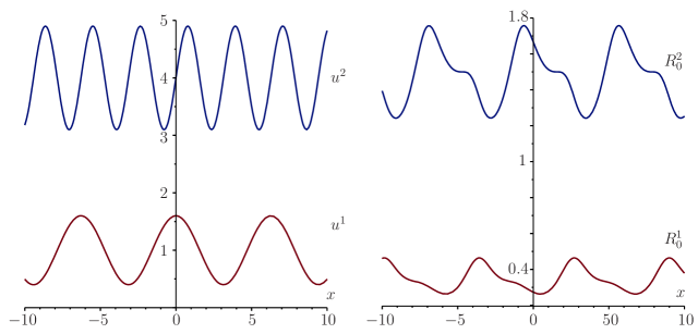
The initial concentration distributions and the corresponding distribution of the Riemann invariants are shown on Fig. 1.

Figure 1: Initial concentrations $u^{1}_{0}(x)$, $u^{2}_{0}(x)$ and the Riemann invariants $R^{1}_{0}(x)$, $R^{2}_{0}(x)$

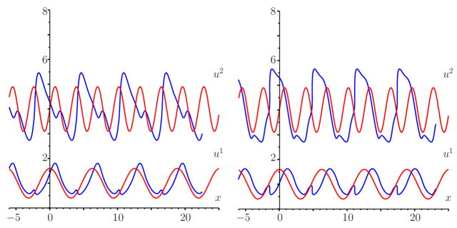
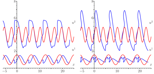
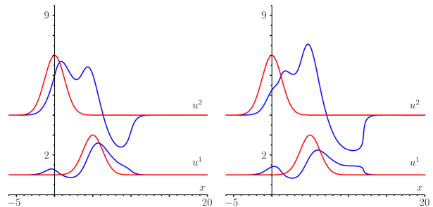
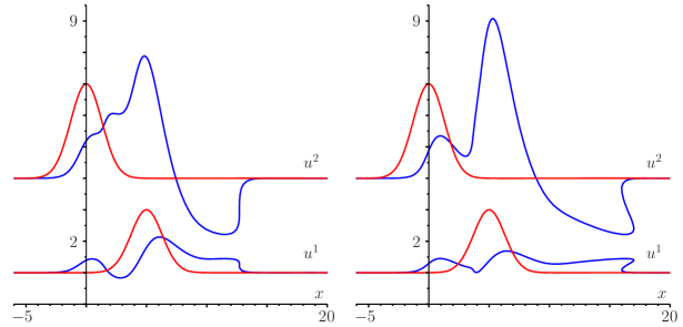
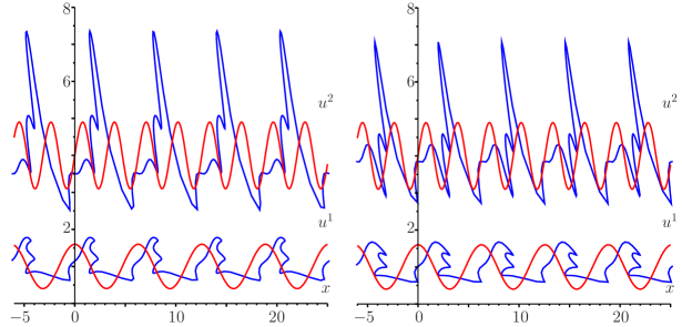
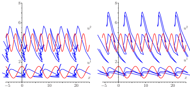
The results of calculations of the functions $u^{1}(x,t)$, $u^{2}(x,t)$ are shown on Fig. 2–5 as $t=1.744$, $2.944$, $3.536$, $6.174$, $8.843$, $10.137$, $14.728$, $21.120$. The red lines correspond to the initial periodic distribution, and the blue lines correspond to the concentration distribution at the appropriate time. For all calculations we use parameter step $\delta\tau=0.05$. We recall that the values $a_{*}$, $b_{*}$ are correspond to isochrone $t_{*}=t(a_{*},b_{*})$ .

Figure 2: (left) $a_{*}=-0.29$, $b_{*}=0.90$, $\delta\tau=0.05$, $x(a_{*},b_{*})=1.106$, $t(a_{*},b_{*})=1.744$; (right) $a_{*}=-1.09$, $b_{*}=0.90$, $\delta\tau=0.05$, $x(a_{*},b_{*})=1.260$, $t(a_{*},b_{*})=2.944$

Figure 3: (left) $a_{*}=-1.29$, $b_{*}=0.90$, $\delta\tau=0.05$, $x(a_{*},b_{*})=1.332$, $t(a_{*},b_{*})=3.536$; (right) $a_{*}=-1.89$, $b_{*}=0.90$, $\delta\tau=0.05$, $x(a_{*},b_{*})=1.623$, $t(a_{*},b_{*})=6.174$

In a real physical situation concentrations $u^{1}(x,t)$, $u^{2}(x,t)$ are one-valued functions of the variable $x$. Thus, the real situation corresponds to time before the moment of the breaking concentration profiles (approximately, $t\approx 3.536$, the first three figires). The remaining figures illustrate the possibilities of the method which allows to construct the multi-valued solutions.

Figure 4: (left) $a_{*}=-6.89$, $b_{*}=0.90$, $\delta\tau=0.05$, $x(a_{*},b_{*})=1.875$, $t(a_{*},b_{*})=8.843$; (right) $a_{*}=-2.89$, $b_{*}=0.90$, $\delta\tau=0.05$, $x(a_{*},b_{*})=2.004$, $t(a_{*},b_{*})=10.137$

Figure 5: (left) $a_{*}=-7.89$, $b_{*}=0.90$, $\delta\tau=0.05$, $x(a_{*},b_{*})=2.580$, $t(a_{*},b_{*})=14.728$; (right) $a_{*}=-9.89$, $b_{*}=0.90$, $\delta\tau=0.05$, $x(a_{*},b_{*})=3.228$, $t(a_{*},b_{*})=21.120$

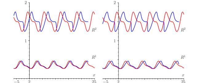
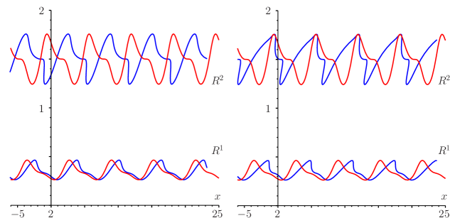
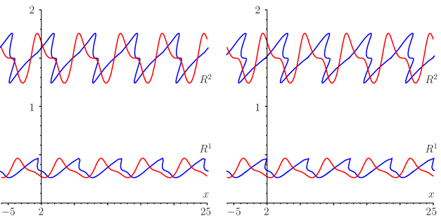
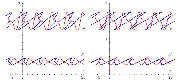
The evolution of the Riemann invariants $R^{1}(x,t)$, $R^{2}(x,t)$ corresponding to Fig. 2–5 is shown on Fig. 6–9. Note that changing of the Riemann invariants $R^{1}$, $R^{2}$ over time is more ‘regular’ than changing of concentrations $u^{1}$, $u^{2}$.

Figure 6: (left) $a_{*}=-0.29$, $b_{*}=0.90$, $\delta\tau=0.05$, $x(a_{*},b_{*})=1.106$, $t(a_{*},b_{*})=1.744$; (right) $a_{*}=-1.09$, $b_{*}=0.90$, $\delta\tau=0.05$, $x(a_{*},b_{*})=1.260$, $t(a_{*},b_{*})=2.944$

Figure 7: (left) $a_{*}=-1.29$, $b_{*}=0.90$, $\delta\tau=0.05$, $x(a_{*},b_{*})=1.332$, $t(a_{*},b_{*})=3.536$; (right) $a_{*}=-1.89$, $b_{*}=0.90$, $\delta\tau=0.05$, $x(a_{*},b_{*})=1.623$, $t(a_{*},b_{*})=6.174$

Figure 8: (left) $a_{*}=-6.89$, $b_{*}=0.90$, $\delta\tau=0.05$, $x(a_{*},b_{*})=1.875$, $t(a_{*},b_{*})=8.843$; (right) $a_{*}=-2.89$, $b_{*}=0.90$, $\delta\tau=0.05$, $x(a_{*},b_{*})=2.004$, $t(a_{*},b_{*})=10.137$

Figure 9: (left) $a_{*}=-7.89$, $b_{*}=0.90$, $\delta\tau=0.05$, $x(a_{*},b_{*})=2.580$, $t(a_{*},b_{*})=14.728$; (right) $a_{*}=-9.89$, $b_{*}=0.90$, $\delta\tau=0.05$, $x(a_{*},b_{*})=3.228$, $t(a_{*},b_{*})=21.120$

III.2.2 Wave packet

We assume that the concentrations $u^{i}$ as time $t=0$ are

$$u^{1}_{0}=u^{1}_{*}(1+\gamma^{1}e^{-\beta^{1}x^{2}}\cos\Omega^{1}x),$$ (3.26)

$$u^{2}_{0}=u^{2}_{*}(1+\gamma^{2}e^{-\beta^{2}x^{2}}\sin\Omega^{2}x),$$

where $u^{i}_{*}$, $\gamma^{i}$, $\Omega^{i}$, $\beta^{i}$ are the constants.

Physically this initial concentration distribution corresponds to the wave packet perturbation.

The results of calculations are given for parameters

$$\mu^{1}=1.0,\quad\mu^{2}=3.0,\quad u^{1}_{*}=1.0,\quad u^{2}_{*}=4.0,\quad\beta^{1}=\beta^{2}=0.1,$$ (3.27)

$$\gamma^{1}=0.1,\quad\gamma^{2}=0.3,\quad\Omega^{1}=5.0,\quad\Omega^{2}=5.0.$$

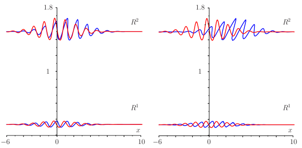
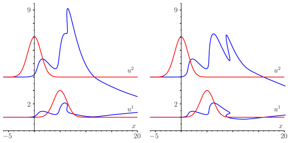
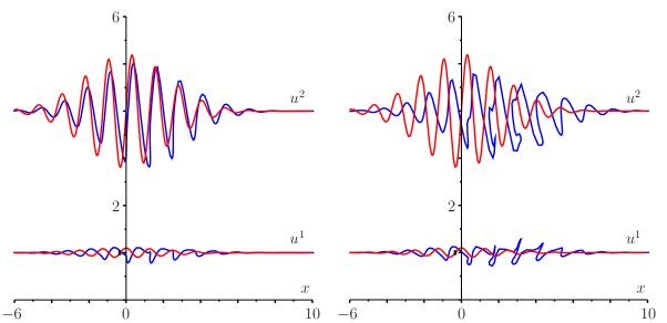
We restrict only an illustration of the calculations for time $t=1.655$, $3.737$. On Fig. 10, 11 the distribution of the concentrations and the Riemann invariants, respectively, are shown. At $t\approx 1.655$ the braking concentration profiles (and, of course, the Riemann invariants) are well visible.

Figure 10: (left) $a_{*}=-0.29$, $b_{*}=0.90$, $\delta\tau=0.05$, $x(a_{*},b_{*})=1.238$, $t(a_{*},b_{*})=1.655$; (right) $a_{*}=-1.29$, $b_{*}=0.90$, $\delta\tau=0.05$, $x(a_{*},b_{*})=1.673$, $t(a_{*},b_{*})=3.737$

Figure 11: (left) $a_{*}=-0.29$, $b_{*}=0.90$, $\delta\tau=0.05$, $x(a_{*},b_{*})=1.238$, $t(a_{*},b_{*})=1.655$; (right) $a_{*}=-1.29$, $b_{*}=0.90$, $\delta\tau=0.05$, $x(a_{*},b_{*})=1.673$, $t(a_{*},b_{*})=3.737$

III.2.3 The Gaussian distribution of the initial concentrations

The initial Gaussian distribution of the concentrations is most often realized in zonal electrophoresis experiments.

We take the following initial data

$$u^{1}_{0}=u^{1}_{*}+\gamma^{1}e^{-\beta^{1}(x-x^{1})^{2}},\quad u^{2}_{0}=u^{2}_{*}+\gamma^{2}e^{-\beta^{2}(x-x^{2})^{2}},$$ (3.28)

where $u^{i}_{*}$, $\gamma^{i}$, $x^{i}$, $\beta^{i}$ are the constants.

The results of calculations are given for parameters

$$\mu^{1}=1.0,\quad\mu^{2}=3.0,\quad u^{1}_{*}=1.0,\quad u^{2}_{*}=4.0,\quad\beta^{1}=\beta^{2}=0.3,$$ (3.29)

$$\gamma^{1}=2.0,\quad\gamma^{2}=3.0,\quad x^{1}=5.0,\quad x^{2}=0.0.$$

On Fig. 12 the isolines of the functions $t(a,b)$, $x(a,b)$ on the plane $(a,b)$ are shown.

Figure 12: The isolines of the function $t(a,b)$ (left) and $x(a,b)$ (right)

On Fig. 13–16 for time moments $t=1,146$, $2.338$,$3.438$, $5.614$, $6.358$, $10.192$, $16.350$, $22.513$ the results of calculations of the functions $u^{k}(x,t)$ are shown. The red lines correspond to the initial distribution, and the blue lines correspond to the concentration distribution in the appropriate time. We use parameter step $\delta\tau=0.05$ for all calculations. We recall that the value $a_{*}$, $b_{*}$ are correspond to isochrone $t_{*}=t(a_{*},b_{*})$ .

Figure 13: (left) $a_{*}=0.49$, $b_{*}=0.90$, $\delta\tau=0.05$, $x(a_{*},b_{*})=1.009$, $t(a_{*},b_{*})=1.146$; (right) $a_{*}=0.09$, $b_{*}=0.90$, $\delta\tau=0.05$, $x(a_{*},b_{*})=1.122$, $t(a_{*},b_{*})=2.338$

Figure 14: (left) $a_{*}=-0.29$, $b_{*}=0.90$, $\delta\tau=0.05$, $x(a_{*},b_{*})=1.226$, $t(a_{*},b_{*})=3.438$; (right) $a_{*}=-1.29$, $b_{*}=0.90$, $\delta\tau=0.05$, $x(a_{*},b_{*})=1.435$, $t(a_{*},b_{*})=5.614$

Figure 15: (left) $a_{*}=-1.89$, $b_{*}=0.90$, $\delta\tau=0.05$, $x(a_{*},b_{*})=1.509$, $t(a_{*},b_{*})=6.358$; (right) $a_{*}=-4.89$, $b_{*}=0.90$, $\delta\tau=0.05$, $x(a_{*},b_{*})=1.921$, $t(a_{*},b_{*})=10.192$

Figure 16: (left) $a_{*}=-8.89$, $b_{*}=0.90$, $\delta\tau=0.05$, $x(a_{*},b_{*})=2.591$, $t(a_{*},b_{*})=16.350$; (right) $a_{*}=-12.89$, $b_{*}=0.90$, $\delta\tau=0.05$, $x(a_{*},b_{*})=3.262$, $t(a_{*},b_{*})=22.513$

We again recall that in a real physical situation the concentrations $u^{1}(x,t)$, $u^{2}(x,t)$ are the one-valued functions of the spatial variable $x$. The real situation corresponds to time before breaking concentration profiles (approximately, $t\approx 6.358$, the first five figures). The remaining figures illustrate the possibilities of the method which allows to construct the multi-valued solutions.

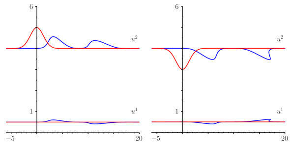
The Fig. 17 shows the results of calculations for the case when the initial data have the form

$$u^{1}_{0}=u^{1}_{*},\quad u^{2}_{0}=u^{2}_{*}+\gamma e^{-\beta x^{2}},$$ (3.30)

$$\mu^{1}=1.0,\quad\mu^{2}=3.0,\quad u^{1}_{*}=0.5,\quad u^{2}_{*}=4.0,\quad\beta=0.3,\quad\gamma=\pm 1.0.$$

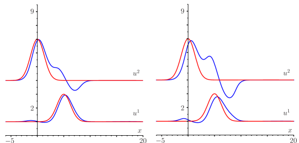
The results illustrate that the presence of the initial perturbation of any only one concentration (in this case $u^{2}$) leads to the perturbation of the other concentrations (in this case $u^{1}$). Strictly speaking, the result is quite obvious, as it is easy to check that the original equation (3.1) does not admit the solutions $u^{1}=\textrm{const}$, $u^{2}\neq\textrm{const}$.

It is interesting to note that the initial Gaussian’s perturbation single peak, in the process of evolution, splits into two peaks. For initial data (3.30), if $\gamma=+1$, the distribution of perturbations occurs quite regularly, whereas in the case $\gamma=-1$, over time there are the breaking concentration profiles, and the occurrence of shock waves.

Figure 17: (left) $\gamma=+1$, $a_{*}=-8.89$, $b_{*}=0.90$, $\delta\tau=0.05$, $x(a_{*},b_{*})=4.268$, $t(a_{*},b_{*})=18.091$; (right) $\gamma=-1$, $a_{*}=-8.89$, $b_{*}=0.90$, $\delta\tau=0.05$, $x(a_{*},b_{*})=6.467$, $t(a_{*},b_{*})=19.942$

IV Conclusions

Implicit solution (3.10), (3.15) of the original problem (2.1), (2.2), of course, is very important in studying of the original Cauchy problem properties. However, from our point of view, the implicit solution is not less complex than the original problem. For practical applications we must get, in one way or another, the explicit relations (2.12). In the general case we need to use a numerical methods, for example, Newton’s method, for solving of the transcendental equations. This, in turn, requires a good initial approximations, or the using of the movement parameter method. It is especially difficult to numerically solve the system (2.10) in the case when original problem has multi-valued solition. In other words, using of the numerical methods of solving the systems of transcendental equations is not much easier than the application of the direct methods for solving of the original problem, for example, using finite difference or finite volume method. Instead solving of the transcendental equations system we propose to solve the Cauchy problem for ODE’s. Even if it is need to solve ODE’s numerically, for example, by the methods of Runge–Kutta method, the numerical algorithm is realized simpler than the algorithm for solving system of nonlinear transcendental equations.

References

• (1) Shiryaeva E. V., Zhukov M. Yu. Hodograph Method and Numerical Solution of the Two Hyperbolic Quasilinear Equations. Part I. Shallow water equations // 2014, arXiv:1410.2832. 19 p.
• (2) Senashov S. I., Yakhno A. Conservation laws, hodograph transformation and boundary value problems of plane plasticity // SIGMA. 2012. Vol. 8, 071. 16 p.
• (3) Rozdestvenskii B. L., Yanenko N. N. Systems of quasilinear equations and their applications to gas dynamics. Providence-Rhode Island: S.n., 1983. 676 p. (American Mathematical Society. Translations of Mathematical Monographs; Vol. 55).
• (4) Whitham G. B. Linear and nonlinear wave. A Wiley-Interscience Publication John Willey & Sons, 1974, New-York–London–Sydney–Toronto.
• (5) El G. A., Kamchatnov A. M. Kinetic equation for a dense soliton gas // ArXiv:nlin/0507016v2. 2006. 4 p.
• (6) Ferapontov E. V., Tsarev S. P. Systems of hydrodynamic type that arise in gas chromatography. Riemann invariants and exact solutions. (Russian) Mat. Model. 3 (1991), no. 2, 82–-91.
• (7) Kuznetsov N. N. Some mathematical questions of chromatography // Computation methohods and programming. 1967. No 6,242–258.
• (8) Elaeva M. S. Investigation of zonal elecrophoresis for two component mixture // (Russian) Mat. Model. 22 (2010), no. 9, 146–-160.
• (9) Elaeva M. S. Separation of two component mixture under action an electric field // Comp. Math. and Mat. Phys. 52:6 (2012), 1143–1159.
• (10) Babskii V. G., Zhukov M. Yu., Yudovich V. I. Mathematical Theory of Electrophoresis. Kluwer Academic / Plenum Publishers (1989).
• (11) Zhukov M. Yu. Non-staionary isotachophoresis model // Comp. Math. and Math. Phys. 1984. V. 24, No 4, 549–565. (in Rissian).
• (12) Zhukov M. Yu. Masstransport by an electric field. Rostov-on-Don: RGU Press, 2005. 215 p.
• (13) Copson E. T. On the Riemann-Green Function // Arch. Ration. Mech. Anal. 1 (1958) 324-348.
• (14) Courant R., Hilbert D. Methods of Mathematical Physics: Partial Differential Equations, Volume II. New York – London, 1964.
• (15) Ibragimov N. Kh. Group analysis of ordinary differential equations and the invariance principle in mathematical physics (for the 150th anniversary of Sophus Lie). // Russian Mathematical Surveys(1992),47(4):89. P. 83–144.
• (16) Chirkunov Yu. A. On the symmetry classification and conservation laws for quasilinear differential equations of second order // Mathematical Notes. 2010, Volume 87, Issue 1–2, pp 115-121.
• (17) Chirkunov Yu. A. Generalized equivalence transformations and group classification of systems of differential equations // Journal of Applied Mechanics and Technical Physics. 2012, Volume 53, Issue 2, pp 147-155.