Radar imaging and characterization of Binary Near-Earth Asteroid (185851) 2000 DP107

Abstract

Potentially hazardous asteroid (185851) 2000 DP107 was the first binary near-Earth asteroid to be imaged. Radar observations in 2000 provided images at 75 m resolution that revealed the shape, orbit, and spin-up formation mechanism of the binary. The asteroid made a more favorable flyby of the Earth in 2008, yielding images at 30 m resolution. We used these data to obtain shape models for the two components and to improve the estimates of the mutual orbit, component masses, and spin periods. The primary has a sidereal spin period of $2.7745\pm 0.0007$ h and is roughly spheroidal with an equivalent diameter of $863$ m $\pm~{}5\%$. It has a mass of $4.656\pm 0.43\times 10^{11}$ kg and a density of $1381\pm 244$ kg m^-3. It exhibits an equatorial ridge similar to the (66391) 1999 KW4 primary, however the equatorial ridge in this case is not as regular and has a $\sim 300$ m diameter concavity on one side. The secondary has a sidereal spin period of 1.77 $\pm$ 0.02 days commensurate with the orbital period. The secondary is slightly elongated and has overall dimensions of $377\times 314\times 268$ m (6% uncertainties). Its mass is $0.178\pm 0.021\times 10^{11}$ kg and its density is $1047\pm 230$ kg m^-3. The mutual orbit has a semi-major axis of $2.659\pm 0.08$ km, an eccentricity of $0.019\pm 0.01$, and a period of $1.7556\pm 0.0015$ days. The normalized total angular momentum of this system exceeds the amount required for the expected spin-up formation mechanism. An increase of angular momentum from non-gravitational forces after binary formation is a possible explanation. The two components have similar radar reflectivity, suggesting a similar composition consistent with formation by spin-up. The secondary appears to exhibit a larger circular polarization ratio than the primary, suggesting a rougher surface or subsurface at radar wavelength scales.

1. Introduction

Asteroid (185851) 2000 DP107 was discovered on 2000 February 29 by the Lincoln Near-Earth Asteroid Research (LINEAR) program in New Mexico. Radar observations in October of that year revealed the asteroid to be a binary system (Margot et al., 2002), the first such system to be imaged in the near-Earth asteroid (NEA) population. The radar data were instrumental in establishing that NEA satellites form by a spin-up and rotational fission process (Margot et al., 2002). Additional radar and photometric studies showed that $\sim 15\%$ of all NEAs larger than 200 m are binary in nature (Pravec et al., 1999; Margot et al., 2002; Pravec et al., 2006). For a recent review of the properties of binary asteroids, see Margot et al. (2015).

The presence of a satellite around the primary gives us an opportunity to secure direct measurements of several quantities that are not normally measurable. Radar observations enable calculations of the orbital period and orbital separation, which reveal the total mass of the binary system through Kepler’s third law. In addition, radar observations enable measurements of the masses of individual components by measuring the distances of the component centers of mass (COMs) from the system COM. Using this information along with the shape models of the two components derived from radar images, we can estimate their densities. These are important constraints for testing models of formation and evolution of NEAs.

Radar observations of 2000 DP107 in 2000 October yielded rough estimates of masses, sizes, and densities of the two components as well as their mutual orbit (Margot et al., 2002). In 2008 September, the asteroid made another close approach to the Earth and was observed at a distance $\sim 0.06$ astronomical units (AU) or about 20 lunar distances. Because this was about half the distance of the 2000 encounter ($\sim 0.11$ AU), it resulted in data sets with signal-to-noise ratio (SNR) $\sim 20$ times higher than in 2000. The high SNRs enabled us to derive component shapes with effective resolutions of $\sim 50$ m on the surface, and estimate the component masses, volumes, and densities more accurately than was possible in Margot et al. (2002).

In this paper we present detailed component shape models, improved estimates of component masses and densities, and estimates of the mutual orbit parameters using the 2000 and the 2008 radar data. This detailed characterization of 2000 DP107 and its favorable accessibility ($\Delta v\approx 5.9$ km s^-1) make it a good candidate for spacecraft rendezvous missions. 2000 DP107 was the target of the PROCYON mission (Funase et al., 2014), which had a planned flyby the asteroid in 2016. However the mission suffered an engine failure and will be unable to perform the flyby.

2. Methods

2.1. Observing and Data Processing

We observed 2000 DP107 using the Arecibo S-band (2380 MHz, 13 cm) radar and the Goldstone X-band (8560 MHz, 3.5 cm) radar on 10 days between 2008 September 9 and 24, during which the asteroid moved $\sim 60^{\circ}$ across the sky. It came closest to Earth on September 11 at a distance of 0.057 AU. Most of the observing time was dedicated to range-Doppler imaging, with the remainder dedicated to collecting continuous wave (CW) spectra. We obtained 335 range-Doppler images and 65 CW spectra using Arecibo and 534 range-Doppler images and 67 CW spectra using Goldstone.

Radar observations were carried out according to the methods described in Naidu et al. (2013). Briefly, radar imaging was carried out by transmitting a repeating pseudo-random code modulated over a circularly polarized carrier wave, using a binary phase shift keying scheme (Proakis and Salehi, 2007). In each run, the waveform was transmitted for approximately the round-trip light-time (RTT) before switching over to the receiver. The received signal was demodulated and then decoded by cross-correlating it with a replica of the transmitted code, yielding a range resolution equal to the baud length of the transmitted code. In each range bin, consecutive returns were fast Fourier transformed (FFT) to obtain the received signal power as a function of Doppler frequency. The end product is a two-dimensional array or image showing the echo power as a function of range and Doppler frequency. Technically, the observable measured at the telescope is the round-trip light time to the target. We obtained range bins by multiplying the baud length of the code by half the speed of light.

For CW runs, a monochromatic wave was transmitted for the RTT to the asteroid before switching over to the receiver. The received signal was demodulated, sampled, and recorded. A FFT was applied to the echo timeseries to obtain the CW spectra.

Table 1 summarizes our observations. Because of the smaller antenna size and transmitter power, the Goldstone data have much lower SNRs ($\sim 1/20$) compared to the Arecibo data. Six to eight consecutive Goldstone runs were summed incoherently in order to improve the SNR.

Table 1Radar Observations of (185851) 2000 DP107 in 2008

Tel	UT Date	Eph	RTT	Ptx	Baud	Prim. res.	Sec. res.	Code	Start-Stop	Runs
	yyyy-mm-dd		s	kW	$\mu$s	Hz	Hz		hhmmss-hhmmss
G	2008-09-09	85	59	445	1.0			127	114323-114719	3
		87			1.0			127	121534-152227	96
					cw	1.0		none	153128-154316	7
G	2008-09-10	89	58	445	cw	1.0		none	100115-100907	5
					0.5			8191	102915-152812	153
					cw	1.0		none	153412-154908	7
A	2008-09-10	89	58	628	cw	0.2		none	101757-102635	5
				611	0.2	0.08	0.04	65535	102829-114008	37
				561	cw	0.2		none	114159-115234	6
A	2008-09-11	89	58	630	cw	0.2		none	094357-095235	5
				616	0.2	0.08	0.04	65535	095452-112810	48
				580	cw	0.2		none	113030-114115	6
G	2008-09-12	89	58	430	cw	1.0		none	095102-100843	10
					0.5			8191	101952-142936	128
					cw	1.0		none	143725-145705	11
A	2008-09-13	89	59	603	cw	0.2		none	084405-085301	5
					0.2	0.08	0.04	65535	085548-105703	57
				570	cw	0.2		none	105927-110823	5
G	2008-09-13	89	59	432	cw	1.0		none	091304-092304	5
					1.0			8191	103240-124441	67
					cw	1.0		none	125127-131326	12
G	2008-09-14	89	60	432	cw	1.0		none	092211-094047	10
					1.0			8191	095318-112614	47
					1.0			8191	114209-130244	40
A	2008-09-15	89	63	$\sim 604$	cw	0.2		none	075347-080310	5
					0.2	0.08	0.04	65535	080616-102000	56
				585	cw	0.2		none	102236-102952	4
A	2008-09-18	89	70	595	cw	0.2		none	065646-070944	6
					0.5	0.24		8191	071531-092200	54
					cw	0.2		none	092751-093340	3
A	2008-09-21	89	81	590	cw	0.2		none	060205-061410	5
				624	0.5	0.24		8191	062313-082654	45
A	2008-09-24	89	93	660	cw	0.2		none	052205-053607	5
				680	1.0			8191	053910-073632	38
				605	cw	0.2		none	073910-075312	5

Note. — The first column indicates the telescope: Arecibo (A) or Goldstone (G). Eph is the ephemeris solution number used. RTT is the round-trip light-time to the target. P_tx is the transmitter power. Baud is the delay (i.e., range) resolution (Bauds of 0.2, 0.5, and 1 $\mu$s correspond to range resolutions of 30, 75, and 150 m respectively). Prim. res. and Sec. res. are the frequency (i.e., Doppler) resolutions of the processed data for the primary and secondary shape modeling respectively. Note that the Doppler spread of the target scales linearly with the transmitter frequency. Code is the length of the pseudo-random code used. The time-span of the received data are listed by their UT start and stop times. The last column indicates the number of runs acquired in each configuration.

2.2. Mutual Orbit

We used a least squares procedure similar to that used in both Margot et al. (2002) and Ostro et al. (2006) to fit Keplerian orbits to the positions of the secondary COM with respect to the primary COM. We used data from 2000 October and 2008 September, and initialized the fitting procedure with thousands of distinct initial conditions spanning the entire range of plausible values for all orbital parameters. From the 2000 data, we selected 2-4 images on each day from September 30 to October 7, or 20 measurement epochs spanning 8 days, yielding 20 range separations and 20 Doppler separations. For the 2008 data set, we measured the component COM separations in 10 Arecibo images on each day of Arecibo observations, and in 6, 3, 6, 2, and 8 Goldstone images on September 9, 10, 11, 12, and 13 respectively, giving us a total of 95 measurement epochs spanning 16 days, or 190 measurements (95 range separations and 95 Doppler separations).

We obtained range-Doppler separations between the primary and secondary COMs using two different techniques. In the first approach we estimated the COM locations in the images by measuring the positions of the leading and trailing edges of the components. In the second approach we relied on shape models obtained with the shape software (Hudson, 1993; Magri et al., 2007) to locate the component COMs. If the shape models are accurate, the second technique can yield superior estimates of the COM positions, and therefore of the mutual orbit parameters. Sections 2.3 and 2.4 describe shape modeling details.

For the first, edge-based approach, we defined leading edges (LE) and trailing edges (TE) in the images on the basis of a 3$\sigma$ signal threshold, where $\sigma$ is the standard deviation of the background noise. The LE was defined as the first range bin where the object had a signal higher than 3$\sigma$ whereas the TE was defined as the last range bin where at least half of the pixels along the Doppler extent exceeded the 3$\sigma$ threshold. The location of this threshold depends on Doppler resolution (shown in Table 1). The primary and secondary were assumed to be roughly spherical and their radii were estimated from radar images to be roughly 450 m and 150 m respectively. With these assumptions the range coordinates of the component COMs were taken to be 450 m and 150 m behind their respective leading edges. The Doppler coordinates of the COMs were assumed to be located in the middle of the Doppler extent on the trailing edge. Conservative uncertainties of 2-3 times the range and Doppler resolutions were assigned to the range-Doppler separations.

For the second, shape-based approach, we used the shape modeling software to locate the component COMs under a uniform density assumption. shape aligns the synthetic radar images derived from the shape models with the observed radar images, and outputs the COM positions used for the alignment with sub-pixel precision. Uncertainties on the order of the image resolution were assigned to the shape-based range and Doppler separations. We computed the COM separations at the same epochs as those used in the edge-based approach.

We fit the mutual orbit and component shapes in an iterative manner. Each iteration started with mutual orbit fitting followed by component shape modeling. In the first iteration, we used the edge-based approach to determine the preliminary mutual orbit and used the orbit solution (orbit pole and longitude of pericenter) to inform our component shape modeling (Sections 2.3 and 2.4). For the second iteration, the best-fit component shapes from the first iteration were used to refine the COM separation estimates using the shape-based approach. These improved primary-secondary separation estimates were used to refine the mutual orbit fit. The refined mutual orbit solution was used to obtain the final shape models of the components.

2.3. Primary Shape

We used the shape software (Hudson, 1993; Magri et al., 2007) to invert the sequence of range-Doppler images and CW spectra from 2008 to obtain a 3D shape model for the primary. Our data set consisted of 278 Arecibo range-Doppler images and 95 CW spectra from both Arecibo and Goldstone covering a 16-day period between 2008 September 9 and 24. We left out the low-resolution Arecibo images from September 24 and all the Goldstone images as they did not improve the quality of the fit and slowed down the shape modeling process. Because we modeled the primary and secondary separately, we edited the images and spectra to exclude the contribution of the other component to the echoes.

Shape modeling was generally carried out in three steps. First we fit a triaxial ellipsoid model to the data to get the overall extents of the object. We then moved on to a 8th-degree-and-order spherical harmonics model to fit for the global-scale topography seen in the images. Finally, in order to fit for the small-scale features, we used a vertex model with 1000 vertices and 1996 triangular facets. This choice yields a facet resolution of $\sim 50$ m, which is comparable to the best range resolution. In each step weighted penalty functions were used to favor models having uniform density, principal axis rotation, and a reasonably smooth surface. We used a cosine law to model the radar scattering from the surface of the asteroid:

$$\frac{d\sigma}{dA}=R(C+1)(\cos{\alpha})^{2C}.$$ (1)

Here $\sigma$ is the radar cross section, $A$ is the target surface area, $R$ is the Fresnel reflectivity, $C$ is a parameter related to the near-surface roughness of the asteroid at the radar wavelength scales, and $\alpha$ is the incidence angle of the wave. Values of $C$ close to 1 represent diffuse scattering, whereas larger values represent more specular scattering (Mitchell et al., 1996).

Because non-linear least-squares methods tend to find local minima when searching a wide parameter space, we carried out an extensive grid search for the best-fit spin axis orientation during the ellipsoid and spherical harmonics shape modeling stages. We assumed that the lightcurve period of 2.775 h (Pravec et al., 2006) provided a good approximation to the sidereal spin period and we fit shape models to the data using spin axis orientations in increments of 15^∘ in ecliptic longitude ($\lambda$) and 15^∘ in ecliptic latitude ($\beta$). For each case, we performed an ellipsoid model fit followed by a 8-degree spherical harmonics model fit. Only the shape parameters, semi-axes in the ellipsoid fit and spherical harmonic coefficients in the spherical harmonic fit, the initial rotational phase of the object, and the radar scattering parameter $R$ were allowed to change. The spin rate, the spin axis orientation, and the radar scattering parameter $C$ were kept fixed. The grid search was repeated for $C$=0.6, 0.8, 1.0, and 1.2. We defined a somewhat arbitrary threshold separating acceptable fits from poorer solutions by visually comparing the synthetic and observed images and using a $\chi_{\nu}^{2}$ threshold of 0.665.

Our mutual orbit pole estimates lie in the region where spin axis orientations were considered acceptable on the basis of the shape model fits. Because we did not obtain a tight constraint on our spin pole using the shape model search (Section 3.2), we used the best-fit mutual orbit pole as the preferred spin pole for shape modeling. For a binary formed by a spin-up process one would expect the primary spin pole to be roughly aligned with the mutual orbit pole, and tidal processes are expected to damp any residual inclination. With this spin pole assumption we fit 8th-degree-and-order spherical harmonics models to the data in the same way as we did in the grid search. Here we tried values of sidereal spin rate ranging from 3111 ^∘/day ($P=2.777$ h) to 3117 ^∘/day ($P=2.772$ h) in steps of 0.2 ^∘/day and values of $C$ ranging from 0.5 to 1.5 in steps of 0.1. As explained in Section 2.2, the shape modeling was done iteratively with the mutual orbit fits: Mutual orbit fits were followed by shape model fits. In the second/final iteration, we performed the spherical harmonics shape model fit followed by a vertex model fit. At each step, we verified the quality of the fit by visually comparing the synthetic data generated by shape with the corresponding observed data. For the vertex model fit we used as initial conditions the best-fit spin state and spherical harmonics shape model determined at the previous step. Once again, only the shape parameters (location of the vertices), the initial rotational phase, and the radar scattering parameter $R$ were allowed to change and all the other parameters were kept fixed.

2.4. Secondary Shape and Spin State

Shape modeling of the secondary component was performed using a method similar to the one described in Section 2.3. The data set for modeling the shape and rotation of the secondary consisted of 180 Arecibo images taken between 2008 September 10 and 15. We left out images with 75 m range resolution from September 18 and 21 because the secondary was barely resolved in these images, and because these images did not improve the quality of the shape model fits. This time it was the primary that was edited out of the images. The CW spectra were not used because we were not able to completely remove the contribution of the primary from the total echo power. We fit an ovoid shape model, followed by a 5th-degree-and-order spherical harmonic model. We then fit a vertex model with 150 vertices and 296 facets.

Periodicities detected in photometric data suggest that the secondary spin period may be close to 1.76 days (Pravec et al., 2006). This can be used as a guide in our shape modeling process, being mindful that lightcurve periods are neither sidereal nor synodic, whereas the shape software uses sidereal spin periods. This periodicity is close to the 1.7556 day orbital period (Table 2), confirming the finding that the secondary is locked in a 1:1 spin-orbit resonance (Margot et al., 2002). We used the radar-derived, sidereal orbital period as the nominal spin period of the secondary for the purpose of shape modeling.

As with the primary, a grid search did not lead to a conclusive result about the spin axis orientation. Absent recent perturbations, one expects the spin pole of a tidally evolved secondary to be closely aligned with the mutual orbit pole, and we used the mutual orbit pole as the spin pole of the secondary. This proximity to the orbit pole can be verified by computing the obliquity of Cassini state 1 (Peale, 1969), which is the state towards which tides drive the satellite spin pole. The other Cassini states are either unstable or the spin of satellite is unstable at those Cassini states (Gladman et al., 1996). The obliquity can be computed by using the following equation derived from Gladman et al. (1996) for a synchronous secondary:

$$\frac{3}{2}\Big{(}\frac{C-\frac{A+B}{2}}{C}\Big{)}\Big{[}\frac{\sin{\theta}\cos{\theta}}{\sin{(\theta\pm i)}}\Big{]}=\Big{(}\frac{\dot{\Omega}}{\omega}\Big{)}.$$ (2)

Here $A<B<C$ are the the principal moments of inertia of the secondary, $\theta$ is the obliquity of the secondary spin pole with respect to the mutual orbit pole, $i$ is the inclination of the mutual orbit with respect to the invariable plane (in this case it is approximately the equatorial plane of the primary), $\dot{\Omega}$ is the precession rate of the mutual orbit, and $\omega$ is the spin rate of the secondary. After the mutual orbit and the primary and the secondary shapes were fit (Sections 3.1, 3.2, and 3.3), we evaluated Equation 2 with the relevant values and found that $\theta<1^{\circ}$, confirming that the expected obliquity is small.

The initial rotation phase was set to a value such that the secondary was oriented with its minimum moment of inertia (MOI) principal axis pointing towards the primary at pericenter. This is the expected configuration of a tidally locked satellite. The same radar scattering law as the one used for the primary was used. We allowed the shape parameters and the radar scattering parameter $R$ to change. The spin rate, the spin axis orientation, and the radar scattering parameter $C$ were kept fixed. During the ovoid model stage, we attempted shape model fits with values of spin period ranging from 1.6 to 1.9 days in steps of 0.01 days.

An elongated and synchronous secondary in an eccentric orbit about the primary exhibits librations, which are oscillations about uniform rotation (eg., Murray and Dermott, 1999). A tidally evolved satellite is expected to exhibit a relaxed-mode libration (Naidu and Margot, 2015), which is equivalent to a forced libration (Murray and Dermott, 1999) when the spin-orbit coupling is negligible. This libration is roughly sinusoidal for small eccentricities and its amplitude as a function of the satellite elongation was estimated by Naidu and Margot (2015) using numerical simulations.

Because the mutual orbit is eccentric ($e\simeq 0.02$) and the secondary is elongated (Sections 3.1 and 3.3), we allowed for the possibility of relaxed-mode libration in longitude in the rotational model. For small amplitudes of forced librations and small orbital eccentricities, the deviation of the secondary orientation from regular circular motion ($\delta\phi$) can be approximated as

$$\delta\phi\approx A_{lib}\sin{[\omega_{\rm f}(t-t_{0})+\pi]},$$ (3)

where $A_{lib}$ is the amplitude of the forced librations, $\omega_{\rm f}$ is the forcing frequency which is equal to the mean orbital motion ($n=2\pi/P$), and $t_{0}$ is the time of pericenter passage. The additional phase of $\pi$ appears because for a synchronous secondary whose natural libration frequency is smaller than the forcing frequency, the librational phase is expected to be $180^{\circ}$ at pericenter (Murray and Dermott, 1999). We repeated the ovoid and spherical harmonics shape model fits with libration amplitudes ranging from 0^∘ to 10^∘ in steps of $1^{\circ}$. We tried all possible libration phases in steps of $4^{\circ}$ in order to cover the libration phase uncertainty which arises due to an almost circular orbit. The libration amplitudes and phases were held at fixed values in each of these fits.

Results of the secondary shape and spin state modeling are discussed in Section 3.3.

2.5. Radar Scattering Properties

We transmitted circularly polarized waves and used two separate channels to receive echoes with the same circular (SC) and opposite circular (OC) polarization as that of the transmitted wave (Ostro, 1993). We summed consecutive Arecibo CW runs from 2008 (Table 1) and measured the power received in the OC and SC channels. The ratio of the power received in SC to the power received in OC yields the circular polarization ratio which is often denoted by $\mu_{C}$. We also used Equation 1 of Ostro (1993) to compute the radar cross-section of the target, which has dimension of surface area. We computed the dimensionless specific radar cross-section ($\hat{\sigma}$), also called the radar albedo, with the OC CW spectra by taking the ratio of the radar cross-section to the geometric cross-sectional area of the target (primary + secondary) at the time of observations. We used shape to compute the orientations of the target and corresponding projected areas at the times of CW runs.

The procedure described in the previous paragraph yielded values of $\hat{\sigma}$ and $\mu_{C}$ that combine the echoes from both the primary and secondary. We were also interested in estimates of these quantities for the secondary component alone. We obtained these by removing the contribution of the primary from the OC CW spectra. This subtraction was performed by fitting a 5th degree polynomial to the primary CW spectra and by masking out the frequency bins that contained contribution from the secondary. After subtraction, we estimated $\hat{\sigma}$ and $\mu_{c}$ for the secondary using the same procedure as that described in the previous paragraph. Results are given in Section 3.4.

2.6. Mass Ratio, Component Masses, and Densities

The COMs of the two components follow roughly Keplerian orbits around the system COM, while the system COM or barycenter orbits the Sun. The motion of the primary COM relative to the system COM is called the reflex motion of the primary. We estimated the mass ratio of the components and the reflex motion of the primary by quantifying the goodness of fit of heliocentric orbit fits using astrometry of the system COM under various mass ratio assumptions.

The system COM lies on the line joining the component COMs at a distance of $d_{p}$ from the primary and a distance of $d_{s}$ from the secondary. The ratio of these distances ($d_{s}/d_{p}$) is equal to the primary-to-secondary mass ratio ($M_{p}/M_{s}$). For a given mass ratio assumption, we calculated the ratio $d_{s}/d_{p}$ and estimated the barycenter locations along the lines joining the component COMs in each of the 278 images obtained in 2008 that were used for shape modeling. This provided estimates of the two-way ranges to the system COM, where we once again used the shape-based component COMs determined to sub-pixel accuracy. We explored mass ratio assumptions from $M_{p}/M_{s}$=15 to 30 in steps of 0.1 to determine the corresponding two-way ranges to the system COM and assigned uncertainties equal to the range resolution. For each mass ratio assumption we then performed a fit for the heliocentric orbit to all available optical astrometry and the system COM ranges. The best overall fit, as indicated by the lowest sum of squares of residuals, yielded an estimate of the actual mass ratio of the system.

We used the mass ratio to apportion the total mass of the system, estimated from the mutual orbit, to the primary and the secondary. These mass estimates were divided by the corresponding component volume estimates, obtained from shape models, to yield component density estimates.

2.7. Primary Gravitational Environment

We used the primary shape model and density estimate to compute the gravity field on the surface of the primary, under a uniform density assumption. The acceleration on the surface is the vector sum of the gravitational acceleration due to the primary’s mass and the centrifugal acceleration due to its spin. An acceleration vector was computed at the center of each facet using the method described in Werner and Scheeres (1997). The gravitational slope, which is the angle that the acceleration vector makes with the local inward-pointing surface-normal vector, was also computed for each facet.

3. Results

3.1. Mutual Orbit

Our shape modeling results showed that the oblateness $J_{2}$ of the primary is about $0.03$ (Section 3.2), such that the difference between observed and osculating orbital elements (Greenberg, 1981) is small. Specifically, the quantity $\frac{3}{2}J_{2}(R_{\rm p}/a)^{2}$ ($R_{\rm p}$ is the primary radius and $a$ is the semimajor axis), which represents the fractional difference between the observed and osculating values of the semi-major axis (Greenberg, 1981), amounts to $\sim 10^{-3}$. If the orbital eccentricity exceeds this value, one can expect an orbital regime where the true and mean anomalies circulate while the longitude of pericenter precesses. For smaller values of the eccentricity, another class of orbit is possible, where the true and mean anomalies librate around pericenter while the longitude of pericenter circulates. For our purposes, both orbit types are well accommodated by fitting the observations to a Keplerian ellipse. However, the orientation of the ellipse may be different for the 2000 and 2008 observations. For reasons explained in Section 4.2, it was not possible to reliably fit for the apsidal precession rate.

The mutual orbit has a semi-major axis $a=2.659\pm 0.08$ km and a sidereal orbital period $P=1.7556\pm 0.0015$ days. Kepler’s third law yields $GM_{T}=32.24\pm 3.00$ m³ s^-2, where $G$ is the gravitational constant and $M_{T}$ is the total mass of the system. Substituting $G=6.67\times 10^{-11}$ m³ kg^-1 s^-2, we find $M_{T}=4.834\pm 0.45\times 10^{11}$ kg. Table 2 lists the best-fit orbital parameters obtained using the combined 2000 and 2008 data and compares it to the values published in Margot et al. (2002). The values from both works are consistent with each other.

Table 2Mutual orbit parameters for 2000 DP107

Parameter	Value from	Value from
	Margot et al. (2002)	this work
Semi-major axis (km)	$2.62\pm 0.16$	$2.659\pm 0.08$
Period (days)	$1.755\pm 0.007$	$1.7556\pm 0.0015$
Eccentricity	$0.01\pm 0.01$	$0.019\pm 0.01$
System mass ($\times 10^{11}$kg)	$4.6\pm 0.5$	$4.834\pm 0.45$
Orbit pole ($\lambda$, $\beta$) (∘)	(283, 67) $\pm$ 10	(294, 78) $\pm$ 10
Reduced $\chi^{2}$	0.32	0.23

3.2. Primary Shape and Spin State

The result of our grid search for the best-fit spin pole is illustrated in Figure 1, which shows a contour plot of the $\chi_{\nu}^{2}$ values of the shape model fits for various orientations of the spin pole. Figure 1 shows the result for $C=0.8$, which gave lower overall $\chi_{\nu}^{2}$ values than the other values of $C$ that we tried. However the general $\chi_{\nu}^{2}$ patterns are similar irrespective of the value of $C$.

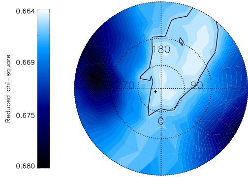
Figure 1.— Contour plot of goodness of fit ($\chi_{\nu}^{2}$) of shape models with different spin axis orientations on a polar stereographic projection of the celestial sphere, looking down the ecliptic north pole. Numbers indicate ecliptic longitudes ($\lambda$). Dotted circles (outside to inside) show latitudes 0^∘, 30^∘, and 60^∘. Region enclosed by solid black contour line ($\chi_{\nu}^{2}=0.665$) shows acceptable shape model fits. Plus sign shows our mutual orbit pole estimate.

As explained in Section 2.3, we assumed the spin pole to be aligned with the mutual orbit pole at $\lambda=294^{\circ}$ and $\beta=78^{\circ}$. The best-fit sidereal spin period is 2.7745 $\pm$ 0.0007 h. Radar scattering $C=1.0$ yielded the shape model with the lowest $\chi_{\nu}^{2}$. Figure 2 shows the vertex shape model produced under these assumptions for the spin pole and the value of $C$, Table 3 lists the associated parameters, and Figure 3 shows examples of the observed images and the fits using this model. The model shows a good general agreement with the data.

An equatorial ridge similar to the one found on the 1999 KW4 primary (Ostro et al., 2006) is clearly seen. However the ridge is not so regular and has a $\sim 300$ m concavity on one side similar to (341843) 2008 EV5 (Busch et al., 2011). An equatorial ridge is necessary to fit the observed power profile behind the leading edge in the radar images. The expected power profiles from models with and without equatorial ridges are compared in Busch et al. (2011). The shape model shows another ridge-like structure forming a ring around the south pole.

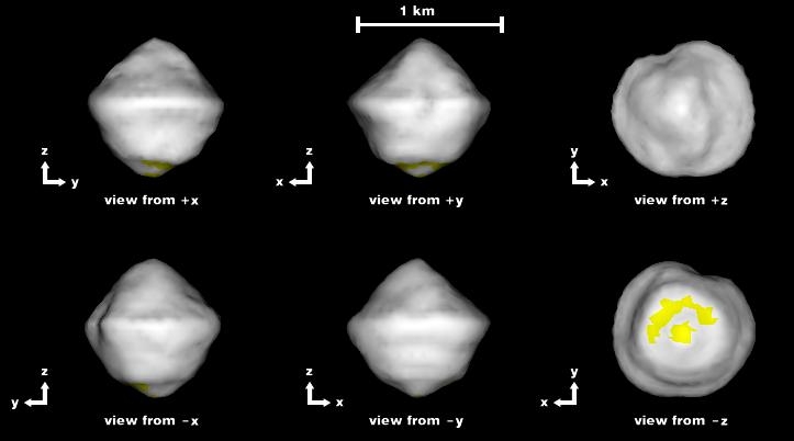
Figure 2.— Vertex shape model of the primary as seen along the three principal axes x, y, and z. For principal axis rotation the spin axis is aligned with the z axis. Yellow regions have radar incidence angles $>60^{\circ}$ and hence are not well constrained. The shape model has 1000 vertices and 1996 triangular facets. The effective surface resolution is $\sim 57$ m.

Table 3Primary and secondary shape model parameters

Parameters		Primary	Secondary
Extents along	x	0.992 $\pm$ 5%	0.379 $\pm$ 6%
principal axes (km)	y	0.938 $\pm$ 5%	0.334 $\pm$ 6%
	z	0.964 $\pm$ 5%	0.270 $\pm$ 6%
Surface area (km2)		2.481 $\pm$ 10%	0.329 $\pm$ 12%
Volume (km3)		0.337 $\pm$ 15%	0.017 $\pm$ 18%
Moment of inertia ratios	$A/C$	0.914 $\pm$ 10%	0.708 $\pm$ 10%
	$B/C$	0.946 $\pm$ 10%	0.888 $\pm$ 10%
Equivalent diameter (km)		0.863 $\pm$ 5%	0.316 $\pm$ 6%
DEEVE extents (km)	x	0.899 $\pm$ 5%	0.377 $\pm$ 6%
	y	0.871 $\pm$ 5%	0.314 $\pm$ 6%
	z	0.821 $\pm$ 5%	0.268 $\pm$ 6%
Spin pole ($\lambda,\beta$) (∘)		(294, 78)	(294, 78)

Note. — The shape model of the primary consists of 1000 vertices and 1996 triangular facets, corresponding to an effective surface resolution of $\sim 57$ m. The shape model of the secondary consists of 150 vertices and 296 facets; it has an effective surface resolution of $\sim$52 m. Surface Area is the surface area of the shape model measured at the model facet scale. The moment of inertia ratios were calculated assuming homogeneous density. $A$, $B$, and $C$ are the principal moments of inertia, such that $A<B<C$. Equivalent diameter is the diameter of a sphere having the same volume as that of the shape model. A dynamically equivalent equal volume ellipsoid (DEEVE) is an ellipsoid with uniform density having the same volume and moment of inertia ratios as the shape model. The spin poles are assumed to be aligned with the mutual orbit pole.

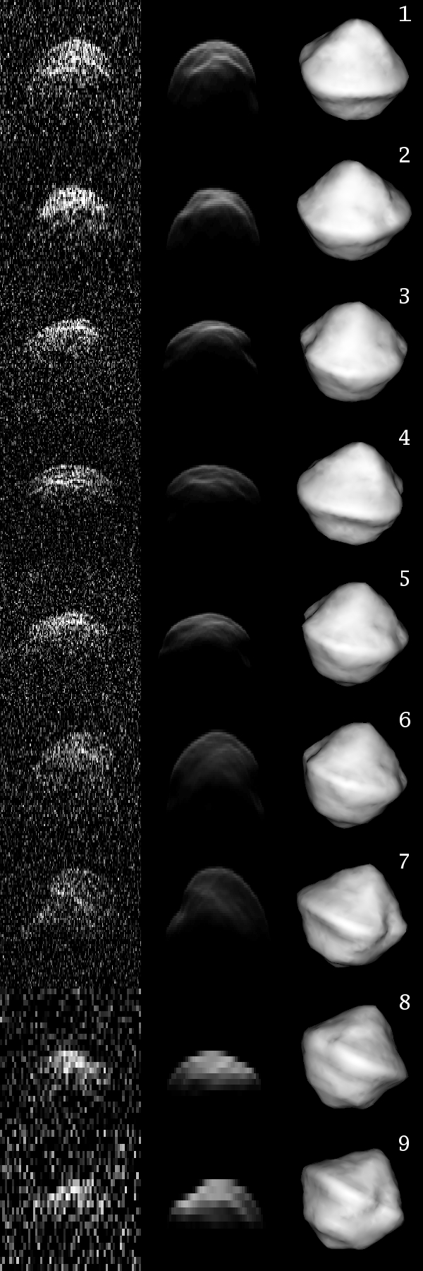
Figure 3.— Examples of images and fits for the primary. Each row (from left to right) shows the observed image (single run), the corresponding synthetic image generated using the shape model, and the corresponding plane of sky view of the shape model. The images were obtained on (from top to bottom) September 10.43641, 10.47739, 11.41307, 11.46787, 13.37204, 15.33765, 15.38140, 18.30239, and 21.26607.

3.3. Secondary Shape and Spin State

We found that including longitudinal libration in the secondary spin model did not improve the shape model fits significantly, so we adopted the shape model fit with no libration as the nominal shape model. The non-detection of libration could either be because the libration amplitude, which is predicted to be $\sim 15$ m by Naidu and Margot (2015), is less than the resolution of the images or the temporal and longitudinal coverage of the secondary is insufficient.

The best-fit sidereal spin period of the secondary is 1.77 $\pm$ 0.02 days. This is consistent with the radar derived mutual orbit period suggesting that the secondary is spinning synchronously. Figure 5 shows the best-fit secondary vertex shape model fit using this period, Table 3 lists the shape model parameters, and Figure 4 shows some examples of the observed images and the fits using this model. There is good agreement between the model and the data. The secondary has a triangular pole-on-silhouette with dynamically equivalent equal volume ellipsoid (DEEVE) dimensions of $377\times 314\times 268$ m.

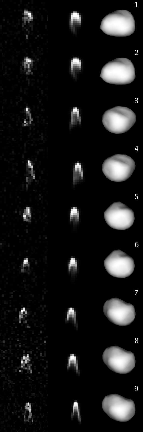
Figure 4.— Examples of images and fits for the secondary. Each row (from left to right) shows the observed image (single run), the corresponding synthetic image generated using the shape model, and the corresponding plane of sky view of the shape model. The images were obtained on (from top to bottom) September 10.47192, 10.48012, 11.41307, 11.44529, 13.43063, 13.43896, 15.33765, 15.36390, and 15.39306.

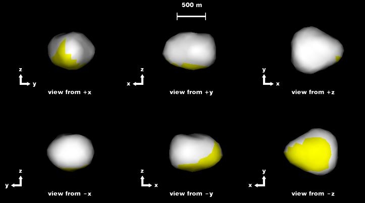
Figure 5.— Secondary shape model as seen along the three principal axes. Top right view is along the positive spin axis. Yellow regions have radar incidence angles $>60^{\circ}$ and hence are not well constrained. The shape model has 150 vertices and 296 triangular facets. The effective surface resolution is $\sim 52$ m.

3.4. Radar Scattering Properties

Measurements of the OC radar albedo and circular polarization ratio for the combined primary and secondary spectra using the Arecibo data obtained in 2008 are listed in Table 4. Their mean values are $0.179\pm 0.02$ and $0.265\pm 0.03$, respectively, where the uncertainties are the standard deviations of the individual measurements. The mean value of circular polarization ratio is close to the median value (0.26) for all NEAs and is most consistent with the S- and C-class asteroids (Benner et al., 2008). Figure 6 shows Arecibo OC and SC CW spectra obtained on 2008 September 11.

Last two columns of Table 4 show the OC radar albedos and circular polarization ratios for the power spectra containing the estimated secondary contribution only. Their mean values are $0.174\pm 0.05$ and $0.326\pm 0.08$, respectively. The radar albedo of the secondary alone is equivalent to that of the primary+secondary, suggesting that both components have identical composition. The polarization ratio of the secondary appears to be more variable and greater than that of the primary, suggesting that the secondary may be rougher than the primary at radar wavelength scales. However, the difference is within the 1 standard deviation of the measurements, preventing a more definite conclusion.

Table 4Radar scattering properties

UT Date	Set	Prim.+Sec.		Secondary
yyyy-mm-dd		$\hat{\sigma}_{\rm OC}$	$\mu_{C}$	$\hat{\sigma}_{\rm OC}$	$\mu_{C}$
2008-09-10	1	0.158	0.334	0.245	0.334
2008-09-10	2	0.239	0.248	0.154	0.238
2008-09-11	1	0.186	0.261	0.098	0.413
2008-09-11	2	0.186	0.258	0.136	0.316
2008-09-13	1	0.197	0.275	0.159	0.458
2008-09-13	2	0.187	0.236	0.226	0.265
2008-09-15	1	0.184	0.241	0.205	0.218
2008-09-15	2	0.159	0.294	0.149	0.373
2008-09-18	1	0.158	0.247	0.125	0.443
2008-09-18	2	0.160	0.242	0.149	0.283
2008-09-21	1	0.180	0.234	0.229	0.254
2008-09-24	1	0.163	0.292	0.176	0.338
2008-09-24	2	0.157	0.276	0.211	0.299
Average		0.179	0.265	0.174	0.326
St. dev.		0.02	0.03	0.05	0.08

Note. — Radar albedos $\hat{\sigma}_{\rm OC}$ and circular polarization ratios $\mu_{C}$ of the primary and secondary combined (columns 3 and 4) and of the secondary alone (columns 5 and 6) measured on the basis of Arecibo data (Table 1). Except for September 21, two measurements were available per day (distinguished by the index in the second column).

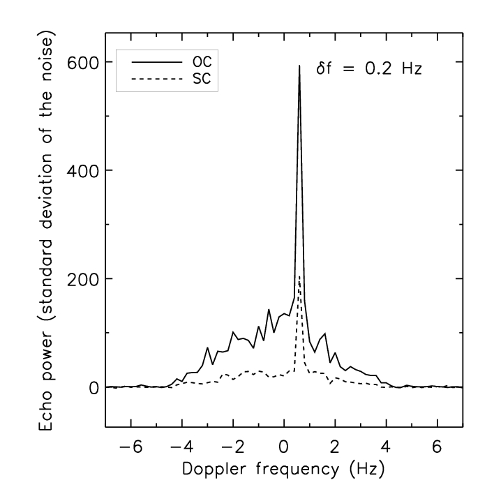
Figure 6.— Representative OC and SC CW spectra obtained at Arecibo on UT 2008 September 11.483. The broad component is due to the primary with 2.77 h spin period. The narrow spike is due to the secondary with 1.77 d spin period.

3.5. Mass Ratio, Component Masses, and Densities

Direct estimation of the mass ratio using the method described in Section 2.6 yielded a mass ratio ($M_{p}/M_{s}$) of 26.2 $\pm$ 2. This mass ratio corresponds to a reflex motion of the primary of 98 $\pm$ 8 m, consistent with the estimate of 140 $\pm$ 40 m of Margot et al. (2002), and with the apparent motion observed directly in the images. Figure 7 shows a plot of the $\chi^{2}$ values of the heliocentric orbit fits to the optical and radar astrometry. The latter uses two-way ranges to the system COM as determined under various mass ratio assumptions as discussed in Section 2.6. Using this mass ratio we can apportion the total mass of the system ($M_{T}$) to the two components. We find the mass of the primary and the secondary to be $4.656\pm 0.43\times 10^{11}$ kg and $0.178\pm 0.021\times 10^{11}$ kg, respectively. Dividing the masses by the volumes of the corresponding shape models, we find densities for the primary and secondary to be $1381\pm 244$ kg m^-3 and $1047\pm 230$ kg m^-3, respectively, where the largest source of uncertainty comes from the volume determinations. The densities are similar, pointing towards a similar composition and porosity.

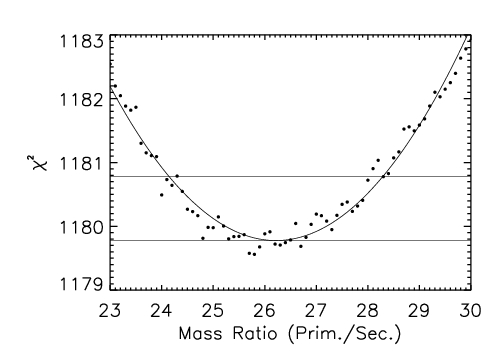
Figure 7.— Points show $\chi^{2}$ values of heliocentric orbit fits to optical and radar astrometric observations. Radar astrometry includes two-way ranges to the system COM under various mass ratio assumptions. Solid curve shows the best fit parabola to the $\chi^{2}$’s. The horizontal lines show the minimum $\chi^{2}$ on the parabola and the $\chi^{2}$ corresponding to the $1\sigma$ uncertainty, respectively. The minimum $\chi^{2}$ corresponds to a primary-to-secondary mass ratio of 26.2 $\pm$ 2.

3.6. Primary Gravitational Environment

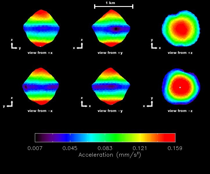
Figure 8.— This figure shows the magnitudes of the vector sum of accelerations due to gravity and centrifugal accelerations computed at the centers of the facets of the primary shape model. We assumed a uniform density of 1381 $\rm{kg~{}m^{-3}}$, which was obtained in Section 3.5, and a spin period of 2.7745 h. At the equator, the values are close to zero, indicating that the magnitude of centrifugal acceleration is almost equal to the magnitude of acceleration due to the asteroid’s mass.

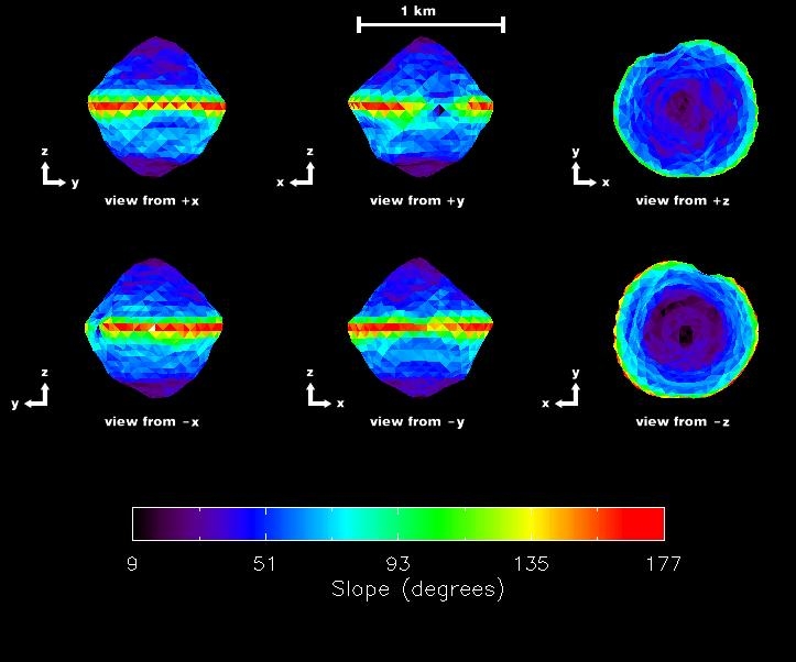
Figure 9.— This figure shows the gravitational slopes computed at the centers of the facets of the primary shape model. We assumed a uniform density of 1381 $\rm{kg~{}m^{-3}}$, obtained in Section 3.5, and a spin period of 2.7745 h. Slopes vary from $\sim 0^{\circ}$ at the poles and some regions at the equator to close to $180^{\circ}$ at most regions at the equator. Most regions at mid-latitudes have slopes between $40^{\circ}$ and $65^{\circ}$.

The acceleration map on the surface of the primary shape model shows that, for nominal values of mass, spin period, and shape parameters, the net acceleration on the equatorial ridge is very close to zero (Figure 8), which implies that the centrifugal acceleration on the ridge almost cancels out the acceleration due to the primary’s mass. As we move to higher latitudes, and hence closer to the spin axis, the magnitude of the centrifugal acceleration decreases, causing the magnitude of the net acceleration to increase and reach values up to 159 $\rm{\mu m~{}s^{-2}}$ at the poles. This value is about 1.6$\times$10^-5 times that on Earth.

The gravitational slopes near the poles are close to zero (Figure 9). Around the mid-latitudes, the slopes are higher and most regions here have values between 40^∘ and 65^∘. Regions on the equatorial ridge have slopes close to 180^∘, implying that the magnitude of centrifugal acceleration is greater than the magnitude of acceleration due to mass. Inside the concavity on the equatorial ridge the slopes are close to $0^{\circ}$. These slopes provide clues to the mechanical properties of the asteroid material. The implications are discussed in Section 4.

4. Discussion

4.1. Primary shape and gravitational environment

The primary shape is similar to shapes of some other radar-characterized asteroids such as (66391) 1999 KW4, (136617) 1994 CC, (341843) 2008 EV5, (101955) Bennu, etc (Ostro et al., 2006; Brozović et al., 2011; Busch et al., 2011; Nolan et al., 2013, respectively). This commonly observed top-shaped structure is an indication that the asteroid has undergone reshaping, most likely due to the spin-up of the primary (e.g., Harris et al., 2009). The shape and the gravitational field provide clues about the mechanical properties of the material of the primary. Figure 9 shows that the gravitational slopes around the mid-latitudes are mostly between 40^∘ and 65^∘. Some of these values are greater than the angle of repose of sand on Earth which has values between 30^∘ and 50^∘. A possible explanation of such high angles is that cohesive van der Waals forces between the particles play an important role on the surfaces of the asteroids as proposed by Scheeres et al. (2010). These cohesive forces could be comparable in magnitude to the ambient gravitational force  (Scheeres et al., 2010), resulting in much higher effective angles of repose ($>50^{\circ}$) that the material can sustain (e.g., Rognon et al., 2008). Figure 9 shows that slopes at the equator of the primary are $>90^{\circ}$, implying that centrifugal force is greater than the gravitational pull at the equator. In the absence of other forces, this imbalance will cause material to escape from the primary at the equator. Cohesion between particles could balance the excess centrifugal force and prevent such an escape. Nevertheless, the regions in the mid-latitudes having high slopes might be devoid of fine grained material, as the material would slide off to lower potential areas. Some of the regions on the equatorial ridge with slopes close to 180^∘ might also be paths through which material is shed off from the primary. The slope values are sensitive to the size, the density, and the spin period of the asteroid. Scaling down the asteroid by $\sim 5\%$ and keeping the mass unchanged (effectively increasing its density by $\sim 16\%$, which is within the density uncertainty) yields slopes close to zero on most regions at the equator and slopes lower than $45^{\circ}$ on most of the surface of the asteroid. If tides and/or YORP spin down the asteroid, there will be a global decrease in the slopes. A similar spin down might have led to the overall low slopes seen on 2008 EV5 (Busch et al., 2011).

Assuming a grain density of 3000 kg m^-3, which would be appropriate for an S-type asteroid, the observed densities of the primary and secondary can be explained by $\sim 55\%$ and $\sim 65\%$ porosity, respectively. Dilation of cohesive materials during avalanching flows seen in numerical simulations and laboratory experiments (e.g., Alexander et al., 2006; Rognon et al., 2008) could also explain the high porosity needed to match the low densities of the primary and the secondary.

The equatorial ridge has an approximately 300 m concavity on it. The concavity could just be a void left over after the asteroid attained its current shape or it could be an impact crater.  Jacobson and Scheeres (2011a) hypothesized that a secondary fission event can take place during the post-fission dynamics following the binary formation process, and that one of the fragments may impact the primary. Secondary fission refers to the rotational fission of the secondary as it is torqued by spin-orbit coupling while in a chaotic rotation state (Jacobson and Scheeres, 2011a; Naidu and Margot, 2015). Gravitational pull dominates the centrifugal force in the interior of the concavity, so ponding of fine grained material transported from higher latitudes can be expected inside the crater.

4.2. Mutual Orbit

The eccentricity of the mutual orbit, $e\approx 0.019$, translates to a variation of the primary-secondary distance of $2ae\approx 100$ m during each orbit. While this variation is detectable in the radar data from 2008, which has a range resolution of $30$ m, it is barely detectable in the radar data obtained in 2000, which has a range resolution of 75 m. Our determination of the longitude of pericenter therefore relies on the 2008 data only. Although we were not able to fit an orbital precession rate, our method does not rule out substantial pericenter precession during 2000-2008. We performed numerical simulations using the method developed by Naidu and Margot (2015) to estimate pericenter precession rates under various gravitational perturbations: the non-spherical mass distribution of the primary causes pericenter precession of about $90^{\circ}$/year, whereas the non-spherical mass distribution of the secondary contributes about $-15^{\circ}$/year. The combined effect causes the pericenter to precess by about $75^{\circ}$/year in a prograde direction with respect to the mutual orbit. Additionally, the gravitational perturbations from the Sun cause the pericenter to precess by about $10^{\circ}$/year. The combined effect of these three gravitational perturbations is a secular apsidal precession rate of about $85^{\circ}$/year, but there are significant short-term variations in the precession rate, making detection of apsidal precession difficult. Gravitational perturbations from planets and radiative forces from the Sun complicate the dynamics further.

The mutual orbit normal (and the assumed primary and secondary spin poles) is separated by about 5^∘ from the heliocentric orbit normal, which is common among binary NEAs and possibly indicative of YORP obliquity evolution (Rubincam, 2000).

4.3. Binary YORP

Binary YORP is a radiative torque which is hypothesized to alter the mutual orbit of synchronous binary systems (Ćuk and Burns, 2005). A synchronous satellite has a fixed leading and trailing side with respect to the direction of its orbital motion, so an asymmetric re-radiation from the surface of the satellite will lead to a net torque on the mutual orbit. A potentially observable signature of such a torqued orbit is a quadratic change in the mean anomaly of the satellite (McMahon and Scheeres, 2010). Detecting a quadratic change in mean anomaly requires measurements of the mean anomaly on a minimum of 3 widely separated epochs. Additional measurements will be required to model the complicated dynamics described in the previous section. 2000 DP107 is a prime candidate for the detection of binary YORP since it presents repeated opportunities for observations and has already been observed in 2000 and 2008 by radar and in 2000, 2008, 2011, and 2013 by optical telescopes. McMahon and Scheeres (2010) made a mean anomaly drift rate prediction for 2000 DP107 by scaling the results obtained from the radar-derived shape model of the satellite of 1999 KW4. Those predictions can now be updated using the secondary shape model. Depending on the direction of the binary YORP torque, the mutual orbit could either expand, contract, or remain unchanged. The outcomes of these scenarios were studied in detail by Jacobson and Scheeres (2011a). An expanding mutual orbit could lead to the formation of asteroid pairs or an asynchronous satellite, whereas a contracting mutual orbit could create a contact binary asteroid (e.g., Taylor and Margot, 2011). A contracting binary YORP torque could also be balanced by an equal and opposite tidal torque implying a binary asteroid in a stable equilibrium as hypothesized by Jacobson and Scheeres (2011b). Future observations of this system may provide a detection of binary YORP evolution.

4.4. Formation and Evolution

The normalized total angular momentum of a binary asteroid system ($J/J^{\prime}$) provides clues to the formation mechanism of the system. In this expression, $J$ is the total angular momentum and $J^{\prime}=\sqrt{GM_{\rm sys}R_{\rm eff}}$, where $M_{\rm sys}$ and $R_{\rm eff}$ are the total mass and equivalent radius of the binary system. Ratios greater than 0.4 in NEAs are consistent with formation of the binary by mass shedding due to spin-up of the parent body (Margot et al., 2002; Pravec and Harris, 2007; Taylor and Margot, 2011). 2000 DP107 has a separation $a/R_{\rm p}\simeq 6.2$ that is larger than most known binary NEAs and a low eccentricity of 0.019, resulting in $J/J^{\prime}\sim 0.49$. This is much larger than is necessary for spin fission. In a tides-only model, this large separation implies a rather weak primary, an old age compared to the dynamical lifetime of NEAs, or the influence of another mechanism such as binary YORP and/or YORP for increasing the total angular momentum (Taylor and Margot, 2011).

5. Conclusion

The radar observations of 2000 DP107 allowed us to produce shape models of the primary and secondary, estimate their masses and densities, compute the gravitational environment of the primary, and estimate the mutual orbit parameters. The shape model and gravitational environment of the primary provide important clues about the material properties of the asteroid. The shape model of the secondary can be used to estimate the evolution of the mutual orbit under the binary YORP torque. Future radar and photometric observations of the system may provide measurements of the evolution of the mutual orbit. The next radar and photometric observation opportunity is in 2016.

6. Acknowledgements

We thank Dan Scheeres and Seth Jacobson for useful discussions, and the anonymous reviewer for excellent suggestions. This material is based upon work supported by the National Science Foundation under Grant No. AST-1211581 and the National Aeronautics and Space Administration under Grant No. NNX14AM95G.

References

- Alexander et al. [2006] Albert W Alexander, Bodhisattwa Chaudhuri, AbdulMobeen Faqih, Fernando J Muzzio, Clive Davies, and M Silvina Tomassone. Avalanching flow of cohesive powders. Powder Technology, 164(1):13–21, 2006.
- Benner et al. [2008] L. A. M. Benner, M. C. Nolan, J. Margot, M. Brozovic, S. J. Ostro, M. K. Shepard, C. Magri, J. D. Giorgini, and M. W. Busch. Arecibo and Goldstone Radar Imaging of Contact Binary Near-Earth Asteroids. In AAS/Division for Planetary Sciences Meeting Abstracts #40, volume 40 of Bulletin of the American Astronomical Society, page 432, September 2008.
- Brozović et al. [2011] M. Brozović, L. A. M. Benner, P. A. Taylor, M. C. Nolan, E. S. Howell, C. Magri, D. J. Scheeres, J. D. Giorgini, J. T. Pollock, P. Pravec, A. Galád, J. Fang, J.-L. Margot, M. W. Busch, M. K. Shepard, D. E. Reichart, K. M. Ivarsen, J. B. Haislip, A. P. LaCluyze, J. Jao, M. A. Slade, K. J. Lawrence, and M. D. Hicks. Radar and optical observations and physical modeling of triple near-Earth Asteroid (136617) 1994 CC. Icarus, 216:241–256, November 2011. 10.1016/j.icarus.2011.09.002.
- Busch et al. [2011] M. W. Busch, S. J. Ostro, L. A. M. Benner, M. Brozovic, J. D. Giorgini, J. S. Jao, D. J. Scheeres, C. Magri, M. C. Nolan, E. S. Howell, P. A. Taylor, J.-L. Margot, and W. Brisken. Radar observations and the shape of near-Earth ASTEROID 2008 EV5. Icarus, 212:649–660, April 2011. 10.1016/j.icarus.2011.01.013.
- Ćuk and Burns [2005] M. Ćuk and J. A. Burns. Effects of thermal radiation on the dynamics of binary NEAs. Icarus, 176:418–431, August 2005. 10.1016/j.icarus.2005.02.001.
- Funase et al. [2014] Ryu Funase, Hiroyuki Koizumi, Shinichi Nakasuka, Yasuhiro Kawakatsu, Yosuke Fukushima, Atsushi Tomiki, Yuta Kobayashi, Junichi Nakatsuka, Makoto Mita, Daisuke Kobayashi, et al. 50kg-class deep space exploration technology demonstration micro-spacecraft procyon. 2014.
- Gladman et al. [1996] B. Gladman, D. D. Quinn, P. Nicholson, and R. Rand. Synchronous Locking of Tidally Evolving Satellites. Icarus, 122:166–192, July 1996. 10.1006/icar.1996.0117.
- Greenberg [1981] R. Greenberg. Apsidal precession of orbits about an oblate planet. Astronomical Journal, 86:912–914, June 1981.
- Harris et al. [2009] A. W. Harris, E. G. Fahnestock, and P. Pravec. On the shapes and spins of rubble pile asteroids. Icarus, 199:310–318, February 2009. 10.1016/j.icarus.2008.09.012.
- Hudson [1993] S. Hudson. Three-dimensional reconstruction of asteroids from radar observations. Remote Sensing Reviews, 8:195–203, 1993.
- Jacobson and Scheeres [2011a] S. A. Jacobson and D. J. Scheeres. Dynamics of rotationally fissioned asteroids: Source of observed small asteroid systems. Icarus, 214:161–178, July 2011a. 10.1016/j.icarus.2011.04.009.
- Jacobson and Scheeres [2011b] S. A. Jacobson and D. J. Scheeres. Long-term Stable Equilibria for Synchronous Binary Asteroids. ApJ, 736:L19, July 2011b. 10.1088/2041-8205/736/1/L19.
- Magri et al. [2007] C. Magri, S. J. Ostro, D. J. Scheeres, M. C. Nolan, J. D. Giorgini, L. A. M. Benner, and J. L. Margot. Radar observations and a physical model of Asteroid 1580 Betulia. Icarus, 186:152–177, January 2007. 10.1016/j.icarus.2006.08.004.
- Margot et al. [2002] J. L. Margot, M. C. Nolan, L. A. M. Benner, S. J. Ostro, R. F. Jurgens, J. D. Giorgini, M. A. Slade, and D. B. Campbell. Binary Asteroids in the Near-Earth Object Population. Science, 296:1445–1448, May 2002. 10.1126/science.1072094.
- Margot et al. [2015] J.-L. Margot, P. Pravec, P. Taylor, B. Carry, and S. Jacobson. Asteroid Systems: Binaries, Triples, and Pairs. ArXiv e-prints, 2015.
- McMahon and Scheeres [2010] J. McMahon and D. Scheeres. Detailed prediction for the BYORP effect on binary near-Earth Asteroid (66391) 1999 KW4 and implications for the binary population. Icarus, 209:494–509, October 2010. 10.1016/j.icarus.2010.05.016.
- Mitchell et al. [1996] D. L. Mitchell, S. J. Ostro, R. S. Hudson, K. D. Rosema, D. B. Campbell, R. Velez, J. F. Chandler, I. I. Shapiro, J. D. Giorgini, and D. K. Yeomans. Radar Observations of Asteroids 1 Ceres, 2 Pallas, and 4 Vesta. Icarus, 124:113–133, November 1996. 10.1006/icar.1996.0193.
- Murray and Dermott [1999] C.D. Murray and S.F. Dermott. Solar System Dynamics. Cambridge University Press, 1999. ISBN 9780521572958. URL http://books.google.co.uk/books?id=NY9iQgAACAAJ.
- Naidu and Margot [2015] S. P. Naidu and J.-L. Margot. Near-Earth Asteroid Satellite Spins Under Spin-orbit Coupling. AJ, 149:80, February 2015. 10.1088/0004-6256/149/2/80.
- Naidu et al. [2013] S. P. Naidu, J.-L. Margot, M. W. Busch, P. A. Taylor, M. C. Nolan, M. Brozovic, L. A. M. Benner, J. D. Giorgini, and C. Magri. Radar imaging and physical characterization of near-Earth Asteroid (162421) 2000 ET70. Icarus, 226:323–335, September 2013. 10.1016/j.icarus.2013.05.025.
- Nolan et al. [2013] M. C. Nolan, C. Magri, E. S. Howell, L. A. M. Benner, J. D. Giorgini, C. W. Hergenrother, R. S. Hudson, D. S. Lauretta, J.-L. Margot, S. J. Ostro, and D. J. Scheeres. Shape model and surface properties of the OSIRIS-REx target Asteroid (101955) Bennu from radar and lightcurve observations. Icarus, 226:629–640, September 2013. 10.1016/j.icarus.2013.05.028.
- Ostro [1993] S. J. Ostro. Planetary radar astronomy. Reviews of Modern Physics, 65:1235–1279, October 1993. 10.1103/RevModPhys.65.1235.
- Ostro et al. [2006] S. J. Ostro, J. L. Margot, L. A. M. Benner, J. D. Giorgini, D. J. Scheeres, E. G. Fahnestock, S. B. Broschart, J. Bellerose, M. C. Nolan, C. Magri, P. Pravec, P. Scheirich, R. Rose, R. F. Jurgens, E. M. De Jong, and S. Suzuki. Radar Imaging of Binary Near-Earth Asteroid (66391) 1999 KW4. Science, 314:1276–1280, November 2006. 10.1126/science.1133622.
- Peale [1969] S. J. Peale. Generalized Cassini’s Laws. AJ, 74:483, April 1969. 10.1086/110825.
- Pravec and Harris [2007] P. Pravec and A. W. Harris. Binary asteroid population. 1. Angular momentum content. Icarus, 190:250–259, September 2007. 10.1016/j.icarus.2007.02.023.
- Pravec et al. [1999] P. Pravec, M. Wolf, and L. Šarounová. How many binaries are there among the near-Earth asteroids? In J. Svoren, E. M. Pittich, and H. Rickman, editors, IAU Colloq. 173: Evolution and Source Regions of Asteroids and Comets, page 159, 1999.
- Pravec et al. [2006] P. Pravec, P. Scheirich, P. Kušnirák, L. Šarounová, S. Mottola, G. Hahn, P. Brown, G. Esquerdo, N. Kaiser, Z. Krzeminski, D. P. Pray, B. D. Warner, A. W. Harris, M. C. Nolan, E. S. Howell, L. A. M. Benner, J. L. Margot, A. Galád, W. Holliday, M. D. Hicks, Y. N. Krugly, D. Tholen, R. Whiteley, F. Marchis, D. R. Degraff, A. Grauer, S. Larson, F. P. Velichko, W. R. Cooney, R. Stephens, J. Zhu, K. Kirsch, R. Dyvig, L. Snyder, V. Reddy, S. Moore, Š. Gajdoš, J. Világi, G. Masi, D. Higgins, G. Funkhouser, B. Knight, S. Slivan, R. Behrend, M. Grenon, G. Burki, R. Roy, C. Demeautis, D. Matter, N. Waelchli, Y. Revaz, A. Klotz, M. Rieugné, P. Thierry, V. Cotrez, L. Brunetto, and G. Kober. Photometric survey of binary near-Earth asteroids. Icarus, 181:63–93, March 2006. 10.1016/j.icarus.2005.10.014.
- Proakis and Salehi [2007] J.G. Proakis and M. Salehi. Digital Communications. McGraw-Hill, 2007. ISBN 9780072957167. URL http://books.google.com/books?id=HroiQAAACAAJ.
- Rognon et al. [2008] P. G. Rognon, J.-N. Roux, M. Naaïm, and F. Chevoir. Dense flows of cohesive granular materials. Journal of Fluid Mechanics, 596:21–47, 2008. 10.1017/S0022112007009329.
- Rubincam [2000] D. P. Rubincam. Radiative Spin-up and Spin-down of Small Asteroids. Icarus, 148:2–11, November 2000. 10.1006/icar.2000.6485.
- Scheeres et al. [2010] D. J. Scheeres, C. M. Hartzell, P. Sánchez, and M. Swift. Scaling forces to asteroid surfaces: The role of cohesion. Icarus, 210:968–984, December 2010. 10.1016/j.icarus.2010.07.009.
- Taylor and Margot [2011] P. A. Taylor and J.-L. Margot. Binary asteroid systems: Tidal end states and estimates of material properties. Icarus, 212:661–676, April 2011. 10.1016/j.icarus.2011.01.030.
- Werner and Scheeres [1997] R. A. Werner and D. J. Scheeres. Exterior Gravitation of a Polyhedron Derived and Compared with Harmonic and Mascon Gravitation Representations of Asteroid 4769 Castalia. Celestial Mechanics and Dynamical Astronomy, 65:313–344, 1997.