High Dimensional Bayesian Optimisation and Bandits via Additive Models

Abstract

Bayesian Optimisation (BO) is a technique used in optimising a $D$-dimensional function which is typically expensive to evaluate. While there have been many successes for BO in low dimensions, scaling it to high dimensions has been notoriously difficult. Existing literature on the topic are under very restrictive settings. In this paper, we identify two key challenges in this endeavour. We tackle these challenges by assuming an additive structure for the function. This setting is substantially more expressive and contains a richer class of functions than previous work. We prove that, for additive functions the regret has only linear dependence on $D$ even though the function depends on all $D$ dimensions. We also demonstrate several other statistical and computational benefits in our framework. Via synthetic examples, a scientific simulation and a face detection problem we demonstrate that our method outperforms naive BO on additive functions and on several examples where the function is not additive.

1 Introduction

In many applications we are tasked with zeroth order optimisation of an expensive to evaluate function $f$ in $D$ dimensions. Some examples are hyper parameter tuning in expensive machine learning algorithms, experiment design, optimising control strategies in complex systems, and scientific simulation based studies. In such applications, $f$ is a blackbox which we can interact with only by querying for the value at a specific point. Related to optimisation is the bandits problem arising in applications such as online advertising and reinforcement learning. Here the objective is to maximise the cumulative sum of all queries. In either case, we need to find the optimum of $f$ using as few queries as possible by managing exploration and exploitation.

Bayesian Optimisation (Mockus & Mockus, 1991) refers to a suite of methods that tackle this problem by modeling $f$ as a Gaussian Process (GP). In such methods, the challenge is two fold. At time step $t$, first estimate the unknown $f$ from the query value-pairs. Then use it to intelligently query at ${{\bf x}_{t}}$ where the function is likely to be high. For this, we first use the posterior GP to construct an acquisition function $\varphi_{t}$ which captures the value of the experiment at a point. Then we maximise $\varphi_{t}$ to determine ${{\bf x}_{t}}$.

Gaussian process bandits and Bayesian optimisation (GPB/ BO) have been successfully applied in many applications such as tuning hyperparameters in learning algorithms (Snoek et al., 2012; Bergstra et al., 2011; Mahendran et al., 2012), robotics (Lizotte et al., 2007; Martinez-Cantin et al., 2007) and object tracking (Denil et al., 2012). However, all such successes have been in low (typically $<10$) dimensions (Wang et al., 2013). Expensive high dimensional functions occur in several problems in fields such as computer vision (Yamins et al., 2013), antenna design (Hornby et al., 2006), computational astrophysics (Parkinson et al., 2006) and biology (Gonzalez et al., 2014). Scaling GPB/ BO methods to high dimensions for practical problems has been challenging. Even current theoretical results suggest that GPB/ BO is exponentially difficult in high dimensions without further assumptions (Srinivas et al., 2010; Bull, 2011). To our knowledge, the only approach to date has been to perform regular GPB/ BO on a low dimensional subspace. This works only under strong assumptions.

We identify two key challenges in scaling GPB/ BO to high dimensions. The first is the statistical challenge in estimating the function. Nonparametric regression is inherently difficult in high dimensions with known lower bounds depending exponentially in dimension (Györfi et al., 2002). The often exponential sample complexity for regression is invariably reflected in the regret bounds for GPB/ BO. The second is the computational challenge in maximising $\varphi_{t}$. Commonly used global optimisation heuristics used to maximise $\varphi_{t}$ themselves require computation exponential in dimension. Any attempt to scale GPB/ BO to high dimensions must effectively address these two concerns.

In this work, we embark on this challenge by treating $f$ as an additive function of mutually exclusive lower dimensional components. Our contributions in this work are:

1. We present the Add-GP-UCB algorithm for optimisation and bandits of an additive function. An attractive property is that we use an acquisition function which is easy to optimise in high dimensions.

2. In our theoretical analysis we bound the regret for Add-GP-UCB. We show that it has only linear dependence on the dimension $D$ when $f$ is additive.

3. Empirically we demonstrate that Add-GP-UCB outperforms naive BO on synthetic experiments, an astrophysical simulator and the Viola and Jones face detection problem. Furthermore Add-GP-UCB does well on several examples when the function is not additive.

A Matlab implementation of our methods is available online at github.com/kirthevasank/add-gp-bandits.

2 Related Work

GPB/ BO methods follow a family of GP based active learning methods which select the next experiment based on the posterior (Osborne et al., 2012; Ma et al., 2015; Kandasamy et al., 2015). In the GPB/ BO setting, common acquisition functions include Expected improvement (Mockus, 1994), probability of improvement (Jones et al., 1998), Thompson sampling (Thompson, 1933) and upper confidence bound (Auer, 2003). Of particular interest to us, is the Gaussian process upper confidence bound (GP-UCB). It was first proposed and analysed in the noisy setting by Srinivas et al. (2010) and extended to the noiseless case by de Freitas et al. (2012). Some literature studies variants, such as combining several acquisition functions (Hoffman et al., 2011) and querying in batches (Azimi et al., 2010).

To our knowledge, most literature for GPB/ BO in high dimensions are in the setting where the function varies only along a very low dimensional subspace (Chen et al., 2012; Wang et al., 2013; Djolonga et al., 2013). In these works, the authors do not encounter either challenge as they perform GPB/ BO in either a random or carefully selected lower dimensional subspace. However, assuming that the problem is an easy (low dimensional) one hiding in a high dimensional space is often too restrictive. Indeed, our experimental results confirm that such methods perform poorly on real applications when the assumptions are not met. While our additive assumption is strong in its own right, it is considerably more expressive. It is more general than the setting in Chen et al. (2012). Even though it does not contain the settings in Djolonga et al. (2013); Wang et al. (2013), unlike them, we still allow the function to vary along the entire domain.

Kernel	Squared Exponential	Matérn
GP-UCB on $D$${}^{\textrm{th}}$ order kernel	$\sqrt{D^{D+2}T(\log T)^{D+2}}$	$2^{D}\sqrt{D}T^{\frac{\nu+D(D+1)}{2\nu+D(D+1)}}\log T$
Add-GP-UCB on additive kernel	$\sqrt{d^{d}D^{2}T(\log T)^{d+2}}$	$2^{d}DT^{\frac{\nu+d(d+1)}{2\nu+d(d+1)}}\log T$

Table 1: Comparison of Cumulative Regret for GP-UCB and Add-GP-UCB for the Squared Exponential and Matérn kernels.

Using an additive structure is standard in high dimensional regression literature both in the GP framework and otherwise. Hastie & Tibshirani (1990); Ravikumar et al. (2009) treat the function as a sum of one dimensional components. Our additive framework is more general. Duvenaud et al. (2011) assume a sum of functions of all combinations of lower dimensional coordinates. These literature argue that using an additive model has several advantages even if $f$ is not additive. It is a well understood notion in statistics that when we only have a few samples, using a simpler model to fit our data may give us a better trade off for estimation error against approximation error. This observation is crucial: in many applications for Bayesian optimisation we are forced to work in the low sample regime since calls to the blackbox are expensive. Though the additive assumption is biased for nonadditive functions, it enables us to do well with only a few samples. While we have developed theoretical results only for additive $f$, empirically we show that our additive model outperforms naive GPB/ BO even when the underlying function is not additive.

Analyses of GPB/ BO methods focus on the query complexity of $f$ which is the dominating cost in relevant applications. It is usually assumed that $\varphi_{t}$ can be maximised to arbitrary precision at negligible cost. Common techniques to maximise $\varphi_{t}$ include grid search, Monte Carlo and multistart methods (Brochu et al., 2010). In our work we use the Dividing Rectangles (DiRect) algorithm of Jones et al. (1993). While these methods are efficient in low dimensions they require exponential computation in high dimensions. It is widely acknowledged in the community that this is a critical bottleneck in scaling GPB/ BO to high dimensions (de Freitas, 2014). While we still work in the paradigm where evaluating $f$ is expensive and characterise our theoretical results in terms of query complexity, we believe that assuming arbitrary computational power to optimise $\varphi_{t}$ is too restrictive. For instance, in hyperparameter tuning the budget for determining the next experiment is dictated by the cost of the learning algorithm. In online advertising and robotic reinforcement learning we need to act in under a few seconds or real time.

In this manuscript, Section 3 formally details our problem and assumptions. We present Add-GP-UCB in Section 4 and our theoretical results in Section 4.3. All proofs are deferred to Appendix B. We summarize the regrets for Add-GP-UCB and GP-UCB in Table 1. In Section 5 we present the experiments.

3 Problem Statement & Set up

We wish to maximise a function $f:\mathcal{X}\rightarrow\mathbb{R}$ where $\mathcal{X}$ is a rectangular region in $\mathbb{R}^{D}$. We will assume w.l.o.g $\mathcal{X}=[0,1]^{D}$. $f$ may be nonconvex and gradient information is not available. We can interact with $f$ only by querying at some $x\in\mathcal{X}$ and obtain a noisy observation $y=f(x)+\epsilon$. Let an optimum point be $\rm{}_{*}=\mathop{\mathrm{argmax}}_{x\in\mathcal{X}}f(x)$. Suppose at time $t$ we choose to query at ${{\bf x}_{t}}$. Then we incur instantaneous regret $r_{t}=f(\rm_{*})-f({{\bf x}_{t}})$. In the bandit setting, we are interested in the cumulative regret $R_{T}=\sum_{t=1}^{T}r_{t}=\sum_{t=1}^{T}f(\rm_{*})-f({{\bf x}_{t}})$, and in the optimisation setting we are interested in the simple regret $S_{T}=\min_{t\leq T}r_{t}=f(\rm_{*})-\max_{{{\bf x}_{t}}}f({{\bf x}_{t}})$. For a bandit algorithm, a desirable property is to have no regret: $\lim_{T\rightarrow\infty}\frac{1}{T}R_{T}=0$. Since $S_{T}\leq\frac{1}{T}R_{T}$, any such procedure is also a consistent procedure for optimisation.

Key structural assumption: In order to make progress in high dimensions, we will assume that $f$ decomposes into the following additive form,

$$f(x)=f^{(1)}(x^{(1)})+f^{(2)}(x^{(2)})+\dots+f^{(M)}(x^{(M)}).$$ (1)

Here each $x^{(j)}\in\mathcal{X}^{(j)}=[0,1]^{d_{j}}$ are lower dimensional components. We will refer to the $\mathcal{X}^{(j)}$’s as “groups” and the grouping of different dimensions into these groups $\{\mathcal{X}^{(j)}\}_{j=1}^{M}$ as the “decomposition”. The groups are disjoint – i.e. if we treat the elements of the vector $x$ as a set, $x^{(i)}\cap x^{(j)}=\varnothing$. We are primarily interestd in the case when $D$ is very large and the group dimensionality is bounded: $d_{j}\leq d\ll D$. We have $D\asymp dM\geq\sum_{j}d_{j}$. Paranthesised superscripts index the groups and a union over the groups denotes the reconstruction of the whole from the groups (e.g. $x=\bigcup_{j}x^{(j)}$ and $\mathcal{X}=\bigcup_{j}\mathcal{X}^{(j)}$). ${{\bf x}_{t}}$ denotes the point chosen by the algorithm for querying at time $t$. We will ignore $\log D$ terms in $\mathcal{O}(\cdot)$ notation. Our theoretical analysis assumes that the decomposition is known but we also present a modified algorithm to handle unknown decompositions and non-additive functions.

Some smoothness assumptions on $f$ are warranted to make the problem tractable. A standard in the Bayesian paradigm is to assume $f$ is sampled from a Gaussian Process (Rasmussen & Williams, 2006) with a covarince kernel $\kappa:\mathcal{X}\times\mathcal{X}\rightarrow\mathbb{R}$ and that $\epsilon\sim\mathcal{N}(0,\eta^{2})$. Two commonly used kernels are the squared exponential (SE) $\kappa_{\sigma,h}$ and the Matérn $\kappa_{\nu,h}$ kernels with parameters $(\sigma,h)$ and $(\nu,h)$ respectively. Writing $r=\|x-x^{\prime}\|_{2}$, they are defined as

$$\kappa_{\sigma,h}(x,x^{\prime}) =\sigma\exp\left(\frac{-r^{2}}{2h^{2}}\right),$$ (2)

$$\kappa_{\nu,h}(x,x^{\prime}) =\frac{2^{1-\nu}}{\Gamma(\nu)}\left(\frac{\sqrt{2\nu}r}{h}\right)^{\nu}B_{\nu}\left(\frac{\sqrt{2\nu}r}{h}\right).$$ (3)

Here $\Gamma,B_{\nu}$ are the Gamma and modified Bessel functions. A principal convenience in modelling our problem via a GP is that posterior distributions are analytically tractable.

In keeping with this, we will assume that each $f^{(j)}$ is sampled from a GP, $\mathcal{G}\mathcal{P}(\mu^{(j)},\kappa^{(j)})$ where the $f^{(j)}$’s are independent. Here, $\mu^{(j)}:\mathcal{X}^{(j)}\rightarrow\mathbb{R}$ is the mean and $\kappa^{(j)}:\mathcal{X}^{(j)}\times\mathcal{X}^{(j)}\rightarrow\mathbb{R}$ is the covariance for $f^{(j)}$. W.l.o.g let $\mu^{(j)}={\bf 0}$ for all $j$. This implies that $f$ itself is sampled from a GP with an additive kernel $\kappa(x,x^{\prime})=\sum_{j}\kappa^{(j)}(x^{(j)},{x^{(j)}}^{\prime})$. We state this formally for nonzero mean as we will need it for the ensuing discussion.

Observation 1.

Let $f$ be defined as in Equation (1), where $f^{(j)}\sim\mathcal{G}\mathcal{P}(\mu^{(j)}(x),\kappa^{(j)}(x^{(i)},{x^{(j)}}^{\prime}))$. Let $y=f(x)+\epsilon$ where $\epsilon~{}\sim\mathcal{N}(0,\eta^{2})$. Denote $\delta(x,x^{\prime})=1\text{ if }x=x^{\prime},\text{ and }0\text{ otherwise}$. Then $y\sim\mathcal{G}\mathcal{P}(\mu(x),\kappa(x,x^{\prime})+\eta^{2}\delta(x,x^{\prime}))$ where

$$\mu(x) =\mu^{(1)}(x^{(1)})+\dots+\mu^{(M)}(x^{(M)})$$ (4)

$$\kappa(x,x^{\prime}) =\kappa^{(1)}(x^{(1)},{x^{(1)}}^{\prime})+\dots+\kappa^{(M)}(x^{(M)},{x^{(M)}}^{\prime}).$$

We will call a kernel such as $\kappa^{(j)}$ which acts only on $d$ variables a $d^{th}$ order kernel. A kernel which acts on all the variables is a $D^{th}$ order kernel. Our kernel for $f$ is a sum of $M$ at most $d^{th}$ order kernels which, we will show, is statistically simpler than a $D^{th}$ order kernel.

We conclude this section by looking at some seemingly straightforward approaches to tackle the problem. The first natural question is of course why not directly run GP-UCB using the additive kernel? Since it is simpler than a $D$${}^{\textrm{th}}$ order kernel we can expect statistical gains. While this is true, it still requires optimising $\varphi_{t}$ in $D$ dimensions to determine the next point which is expensive.

Alternatively, for an additive function, we could adopt a sequential approach where we use $1/M$ fraction of our query budget to maximise the first group by keeping the rest of the coordinates constant. Then we proceed to the second group and so on. While optimising a $d$ dimensional acquisition function is easy, this approach is not desirable for several reasons. First, it will not be an anytime algorithm as we will have to pre-allocate our query budget to maximise each group. Once we proceed to a new group we cannot come back and optimise an older one. Second, such an approach places too much faith in the additive assumption. We will only have explored $M$ $d$-dimensional hyperplanes in the entire space. Third, it is not suitable as a bandit algorithm as we suffer high regret until we get to the last group. We further elaborate on the deficiencies of this and other sequential approaches in Appendix A.2.

4 Algorithm

Under an additive assumption, our algorithm has two components. First, we obtain the posterior GP for each $f^{(j)}$ using the query-value pairs until time $t$. Then we maximise a $d$ dimensional GP-UCB-like acquisition function on each GP to construct the next query point. Since optimising $\varphi_{t}$ depends exponentially in dimension, this is cheaper than optimising one acquisition on the combined GP.

Figure 1: Illustration of the additive GP model for $2$ observations where $M=2$ in (1). The squared variables are observed while the circled variables are not. For brevity we have denoted $f^{(j)}_{i}=f^{(j)}(x^{(j)}_{i})$ for $i=1,2,*$. We wish to infer the posterior distributions of the individual GPs $f^{(j)}(x^{(j)}_{*})$ (outlined in blue).

4.1 Inference on Additive GPs

Typically in GPs, given noisy labels, $Y=\{y_{1},\dots,y_{n}\}$ at points $X=\{x_{1},\dots,x_{n}\}$, we are interested in inferring the posterior distribution for $f_{*}=f(x_{*})$ at a new point $x_{*}$. In our case though, we will be primarily interested in the distribution of $f^{(j)}_{*}=f^{(j)}(x^{(j)}_{*})$ conditioned on $X,Y$. We have illustrated this graphically in Figure 1. The joint distribution of $f^{(j)}_{*}$ and $Y$ can be written as

$$\left(\!\!\!\begin{array}[]{c}f^{(j)}_{*}\\ Y\end{array}\!\!\!\right)\;\sim\mathcal{N}\left({\bf 0},\left[\!\!\!\begin{array}[]{cccc}\kappa^{(j)}(x^{(j)}_{*},x^{(j)}_{*})&\kappa^{(j)}(x^{(j)}_{*},X^{(j)})\\ \kappa^{(j)}(X^{(j)},x^{(j)}_{*})&\kappa(X,X)+\eta^{2}I_{n}\end{array}\!\!\!\right]\right).$$

The $p$${}^{\textrm{th}}$ element of $\kappa^{(j)}(X^{(j)},x^{(j)}_{*})\in\mathbb{R}^{n}$ is $\kappa(x^{(j)}_{p},x^{(j)}_{*})$ and the $(p,q)$${}^{\textrm{th}}$ element of $\kappa(X,X)\in\mathbb{R}^{n\times n}$ is $\kappa(x_{p},x_{q})$. We have used the fact $\operatorname*{Cov}(f^{(i)}_{*},y_{p})=\operatorname*{Cov}(f^{(i)}_{*},\sum_{j}f^{(j)}(x^{(j)}_{p})+\eta^{2}\epsilon)=\operatorname*{Cov}(f^{(i)}_{*},f^{(i)}(x^{(i)}_{p}))=\kappa^{(i)}(x^{(i)}_{*},x^{(i)}_{p})$ as $f^{(j)}\perp f^{(i)},\forall i\neq j$. By writing $\Delta=\kappa(X,X)+\eta^{2}I_{n}\in\mathbb{R}^{n\times n}$, the posterior for $f^{(j)}_{*}$ is,

$$f^{(j)}_{*}|x_{*},X,Y\,\sim\,\mathcal{N}\big{(}\kappa^{(j)}(x^{(j)}_{*},X^{(j)})\Delta^{-1}Y,$$ (5)

$$\hskip 14.45377pt\kappa^{(j)}(x^{(j)}_{*},x^{(j)}_{*})-\kappa^{(j)}(x^{(j)}_{*},X^{(j)})\Delta^{-1}\kappa^{(j)}(X,x^{(j)})\big{)}$$

4.2 The Add-GP-UCB Algorithm

In GPB/ BO algorithms, at each time step $t$ we maximise an acquisition function $\varphi_{t}$ to determine the next point: ${{\bf x}_{t}}=\mathop{\mathrm{argmax}}_{x\in\mathcal{X}}\varphi_{t}(x)$. The acquisition function is itself constructed using the posterior GP. The GP-UCB acquisition function, which we focus on here is,

$$\varphi_{t}(x)=\mu_{t-1}(x)+\beta_{t}^{1/2}\sigma_{t-1}(x).$$

Intuitively, the $\mu_{t-1}$ term in the GP-UCB objective prefers points where $f$ is known to be high, the $\sigma_{t-1}$ term prefers points where we are uncertain about $f$ and $\beta_{t}^{1/2}$ negotiates the tradeoff. The former contributes to the “exploitation” facet of our problem, in that we wish to have low instantaneous regret. The latter contributes to the “exploration” facet since we also wish to query at regions we do not know much about $f$ lest we miss out on regions where $f$ is high. We provide a brief summary of GP-UCB and its theoretical properties in Appendix A.1.

As we have noted before, maximising $\varphi_{t}$ which is typically multimodal to obtain ${{\bf x}_{t}}$ is itself a difficult problem. In any grid search or branch and bound methods such as DiRect, maximising a function to within $\zeta$ accuracy, requires $\mathcal{O}(\zeta^{-D})$ calls to $\varphi_{t}$. Therefore, for large $D$ maximising $\varphi_{t}$ is extremely difficult. In practical settings, especially in situations where we are computationally constrained, this poses serious limitations for GPB/ BO as we may not be able to optimise $\varphi_{t}$ to within a desired accuracy.

Fortunately, in our setting we can be more efficient. We propose an alternative acquisition function which applies to an additive kernel. We define the Additive Gaussian Process Upper Confidence Bound (Add-GP-UCB) to be

$$\widetilde{\varphi}_{t}(x)=\mu_{t-1}(x)+\beta_{t}^{1/2}\sum_{j=1}^{M}\sigma^{(j)}_{t-1}(x^{(j)}).$$ (6)

We immediately see that we can write $\widetilde{\varphi}_{t}$ as a sum of functions on orthogonal domains: $\widetilde{\varphi}_{t}(x)=\sum_{j}\widetilde{\varphi}_{t}^{(j)}(x^{(j)})$ where $\widetilde{\varphi}_{t}^{(j)}(x^{(j)})=\mu^{(j)}_{t-1}(x^{(j)})+\beta_{t}^{1/2}\sigma^{(j)}_{t-1}(x^{(j)})$. This means that $\widetilde{\varphi}_{t}$ can be maximised by maximising each $\widetilde{\varphi}_{t}^{(j)}$ separately on $\mathcal{X}^{(j)}$. As we need to solve $M$ at most $d$ dimensional optimisation problems, it requires only $\mathcal{O}(M^{d+1}\zeta^{-d})$ calls to the utility function in total – far more favourable than maximising $\varphi_{t}$.

Since the cost for maximising the acquisition function is a key theme in this paper let us delve into this a bit more. One call to $\varphi_{t}$ requires $\mathcal{O}(Dt^{2})$ effort. For $\widetilde{\varphi}_{t}$ we need $M$ calls each requiring $\mathcal{O}(d_{j}t^{2})$ effort. So both $\varphi_{t}$ and $\widetilde{\varphi}_{t}$ require the same effort in this front. For $\varphi_{t}$, we need to know the posterior for only $f$ whereas for $\widetilde{\varphi}_{t}$ we need to know the posterior for each $f^{(j)}$. However, the brunt of the work in obtaining the posterior is the $\mathcal{O}(t^{3})$ effort in inverting the $t\times t$ matrix $\Delta$ in (5) which needs to be done for both $\varphi_{t}$ and $\widetilde{\varphi}_{t}$. For $\widetilde{\varphi}_{t}$, we can obtain the inverse once and reuse it $M$ times, so the cost of obtaining the posterior is $\mathcal{O}(t^{3}+Mt^{2})$. Since the number of queries needed will be super linear in $D$ and hence $M$, the $t^{3}$ term dominates. Therefore obtaining each posterior $f^{(j)}$ is only marginally more work than obtaining the posterior for $f$. Any difference here is easily offset by the cost for maximising the acquisition function.

The question remains then if maximising $\widetilde{\varphi}_{t}$ would result in low regret. Since $\varphi_{t}$ and $\widetilde{\varphi}_{t}$ are neither equivalent nor have the same maximiser it is not immediately apparent that this should work. Nonetheless, intuitively this seems like a reasonable scheme since the $\sum_{j}\sigma^{(j)}_{t-1}$ term captures some notion of the uncertainty and contributes to exploration. In Theorem 5 we show that this intuition is reasonable – maximising $\widetilde{\varphi}_{t}$ achieves the same rates as $\varphi_{t}$ for cumulative and simple regrets if the kernel is additive.

We summarise the resulting algorithm in Algorithm 1. In brief, at time step $t$, we obtain the posterior distribution for $f^{(j)}$ and maximise $\widetilde{\varphi}_{t}^{(j)}$ to determine the coordinates ${\bf x}_{t}^{(j)}$. We do this for each $j$ and then combine them to obtain ${{\bf x}_{t}}$.

Input: Kernels $\kappa^{(1)},\dots,\kappa^{(M)}$, Decomposition $(\mathcal{X}^{(j)})_{j=1}^{M}$

• $\mathcal{D}_{0}\leftarrow\varnothing$,

• for $j=1,\dots,M$, $(\mu^{(j)}_{0},\kappa^{(j)}_{0})\leftarrow({\bf 0},\kappa^{(j)})$.

• for $t=1,2,\dots$

  1. for $j=1,\dots,M$,
         ${\bf x}_{t}^{(j)}\leftarrow\mathop{\mathrm{argmax}}_{z\in\mathcal{X}^{(j)}}\mu^{(j)}_{t-1}(z)+\sqrt{\beta_{t}}\sigma^{(j)}_{t-1}(z)$

  2. ${{\bf x}_{t}}\leftarrow\bigcup_{j=1}^{M}{\bf x}_{t}^{(j)}$.

  3. ${{\bf y}_{t}}\leftarrow\textrm{Query $f$ at ${{\bf x}_{t}}$}$.

  4. $\mathcal{D}_{t}=\mathcal{D}_{t-1}\cup\{({{\bf x}_{t}},{{\bf y}_{t}})\}$.

  5. Perform Bayesian posterior updates conditioned on $\mathcal{D}_{t}$ to obtain $\mu^{(j)}_{t},\sigma^{(j)}_{t}$ for $j=1,\dots,M$.

Algorithm 1 Add-GP-UCB

4.3 Main Theoretical Results

Now, we present our main theoretical contributions. We bound the regret for Add-GP-UCB under different kernels. Following Srinivas et al. (2010), we first bound the statistical difficulty of the problem as determined by the kernel. We show that under additive kernels the problem is much easier than when using a full $D$${}^{\textrm{th}}$ order kernel. Next, we show that the Add-GP-UCB algorithm is able to exploit the additive structure and obtain the same rates as GP-UCB. The advantage to using Add-GP-UCB is that it is much easier to optimise the acquisition function. For our analysis, we will need Assumption 2 and Definition 3.

Assumption 2.

Let $f$ be sampled from a GP with kernel $\kappa$. $\kappa(\cdot,x)$ is $L$-Lipschitz for all $x$. Further, the partial derivatives of $f$ satisfies the following high probability bound. There exists constants $a,b>0$ such that,

$$\mathbb{P}\left(\sup_{x}\Big{|}\frac{\partial f(x)}{\partial x_{i}}\Big{|}>J\right)\leq ae^{-(J/b)^{2}}.$$

The Lipschitzian condition is fairly mild and the latter condition holds for four times differentiable stationary kernels such as the SE and Matérn kernels for $\nu>2$ (Ghosal & Roy, 2006). Srinivas et al. (2010) showed that the statistical difficulty of GPB/ BO is determined by the Maximum Information Gain as defined below. We bound this quantity for additive SE and Matérn kernels in Theorem 4. This is our first main theorem.

Definition 3.

(Maximum Information Gain) Let $f\sim\mathcal{G}\mathcal{P}(\mu,\kappa)$, $y_{i}=f(x_{i})+\epsilon$ where $\epsilon\sim\mathcal{N}(0,\eta^{2})$. Let $A=\{x_{1},\dots,x_{T}\}\subset\mathcal{X}$ be a finite subset, $f_{A}$ denote the function values at these points and $y_{A}$ denote the noisy observations. Let $I$ be the Shannon Mutual Information. The Maximum Information Gain between $y_{A}$ and $f_{A}$ is

$$\gamma_{T}=\max_{A\subset\mathcal{X},|A|=T}I(y_{A};f_{A}).$$

Theorem 4.

Assume that the kernel $\kappa$ has the additive form of (4), and that each $\kappa^{(j)}$ satisfies Assumption 2. W.l.o.g assume $\kappa(x,x^{\prime})=1$. Then,

1. If each $\kappa^{(j)}$ is a $d_{j}^{th}$ order squared exponential kernel (2) where $d_{j}\leq d$, then $\gamma_{T}\in\mathcal{O}(Dd^{d}(\log T)^{d+1})$.

2. If each $\kappa^{(j)}$ is a $d_{j}^{th}$ order Matérn kernel (3) where $d_{j}\leq d$ and $\nu>2$, then $\gamma_{T}\in\mathcal{O}(D2^{d}T^{\frac{d(d+1)}{2\nu+d(d+1)}}\log(T))$.

We use bounds on the eigenvalues of the SE and Matérn kernels from Seeger et al. (2008) and a result from Srinivas et al. (2010) which bounds the information gain via the eigendecay of the kernel. We bound the eigendecay of the sum $\kappa$ via $M$ and the eigendecay of a single $\kappa^{(j)}$. The complete proof is given in Appendix B.1. The important observation is that the dependence on $D$ is linear for an additive kernel. In contrast, for a $D$${}^{\textrm{th}}$ order kernel this is exponential (Srinivas et al., 2010).

Next, we present our second main theorem which bounds the regret for Add-GP-UCB for an additive kernel as given in Equation 4.

Theorem 5.

Suppose $f$ is constructed by sampling $f^{(j)}\sim\mathcal{G}\mathcal{P}({\bf 0},\kappa^{(j)})$ for $j=1,\dots,M$ and then adding them. Let all kernels $\kappa^{(j)}$ satisfy assumption 2 for some $L,a,b$. Further, we maximise the acquisition function $\widetilde{\varphi}_{t}$ to within $\zeta_{0}t^{-1/2}$ accuracy at time step $t$. Pick $\delta\in(0,1)$ and choose

$$\beta_{t} =2\log\left(\frac{M\pi^{2}t^{2}}{2\delta}\right)+2d\log\left(Dt^{3}\right)\in\;\mathcal{O}\left(d\log t\right).$$

Then, Add-GP-UCB attains cumulative regret $R_{T}\in\mathcal{O}\left(\sqrt{\vphantom{T^{1}}D\gamma_{T}T\log T}\right)$ and hence simple regret $S_{T}\in\mathcal{O}\left(\sqrt{\vphantom{T^{1}}D\gamma_{T}\log T/T}\right)$. Precisely, with probability $>1-\delta$,

$$\forall T\geq 1,\;\;\;R_{T}\leq\sqrt{8C_{1}\beta_{T}MT\gamma_{t}}+2\zeta_{0}\sqrt{T}+C_{2}.$$

where $C_{1}=1/\log(1+\eta^{-2})$ and $C_{2}$ is a constant depending on $a$, $b$, $D$, $\delta$, $L$ and $\eta$.

Part of our proof uses ideas from Srinivas et al. (2010). We show that $\sum_{j}\beta_{t}\sigma^{(j)}_{t-1}(\cdot)$ forms a credible interval for $f(\cdot)$ about the posterior mean $\mu_{t}(\cdot)$ for an additive kernel in Add-GP-UCB. We relate the regret to this confidence set using a covering argument. We also show that our regret doesn’t suffer severely if we only approximately optimise the acquisition provided that the accuracy improves at rate $\mathcal{O}(t^{-1/2})$. For this we establish smoothness of the posterior mean. The correctness of the algorithm follows from the fact that Add-GP-UCB can be maximised by individually maximising $\widetilde{\varphi}_{t}^{(j)}$ on each $\mathcal{X}^{(j)}$. The complete proof is given in Appendix B.2. When we combine the results in Theorems 4 and 5 we obtain the rates given in Table 1.

One could consider alternative lower order kernels – one candidate is the sum of all possible $d^{th}$ order kernels (Duvenaud et al., 2011). Such a kernel would arguably allow us to represent a larger class of functions than our kernel in (4). If, for instance, we choose each of them to be a SE kernel, then it can be shown that $\gamma_{T}\in\mathcal{O}(D^{d}d^{d+1}(\log T)^{d+1})$. Even though this is worse than our kernel in $\textrm{poly}(D)$ factors, it is still substantially better than using a $D$${}^{\textrm{th}}$ order kernel. However, maximising the corresponding utility function, either of the form $\varphi_{t}$ or $\widetilde{\varphi}_{t}$, is still a $D$ dimensional problem. We reiterate that what renders our algorithm attractive in large $D$ is not just the statistical gains due to the simpler kernel. It is also the fact that our acquisition function can be efficiently maximised.

4.4 Practical Considerations

Our practical implementation differs from our theoretical analysis in the following aspects.

Choice of $\beta_{t}$: $\beta_{t}$ as specified by Theorems 5, usually tends to be conservative in practice (Srinivas et al., 2010). For good empirical performance a more aggressive strategy is required. In our experiments, we set $\beta_{t}=0.2d\log(2t)$ which offered a good tradeoff between exploration and exploitation. Note that this captures the correct dependence on $D,d$ and $t$ in Theorems 5 and 6.

Data dependent prior: Our analysis assumes that we know the GP kernel of the prior. In reality this is rarely the case. In our experiments, we choose the hyperparameters of the kernel by maximising the GP marginal likelihood (Rasmussen & Williams, 2006) every $N_{cyc}$ iterations.

Initialisation: Marginal likelihood based kernel tuning can be unreliable with few data points. This is a problem in the first few iterations. Following the recommendations in Bull (2011) we initialise Add-GP-UCB (and GP-UCB) using $N_{init}$ points selected uniformly at random.

Decomposition & Non-additive functions: If $f$ is additive and the decomposition is known, we use it directly. But it may not always be known or $f$ may not be additive. Then, we could treat the decomposition as a hyperparameter of the additive kernel and maximise the marginal likelihood w.r.t the decomposition. However, given that there are $D!/{d!}^{M}M!$ possible decompositions, computing the marginal likelihood for all of them is infeasible. We circumvent this issue by randomly selecting a few ($\mathcal{O}(D)$) decompositions and choosing the one with the largest marginal likelihood. Intuitively, if the function is not additive, with such a “partial maximisation” we can hope to capture some existing marginal structure in $f$. At the same time, even an exhaustive maximisation will not do much better than a partial maximisation if there is no additive structure. Empirically, we found that partially optimising for the decomposition performed slightly better than using a fixed decomposition or a random decomposition at each step. We incorporate this procedure for finding an appropriate decomposition as part of the kernel hyper parameter learning procedure every $N_{cyc}$ iterations.

How do we choose $(d,M)$ when $f$ is not additive? If $d$ is large we allow for richer class of functions, but risk high variance. For small $d$, the kernel is too simple and we have high bias but low variance – further optimising $\widetilde{\varphi}_{t}$ is easier. In practice we found that our procedure was fairly robust for reasonable choices of $d$. Yet this is an interesting theoretical question. We also believe it is a difficult one. Using the marginal likelihood alone will not work as the optimal choice of $d$ also depends on the computational budget for optimising $\widetilde{\varphi}_{t}$. We hope to study this question in future work. For now, we give some recommendations at the end. Our modified algorithm with these practical considerations is given below. Observe that in this specification if we use $d=D$ we have the original GP-UCB algorithm.

Input: $N_{init}$, $N_{cyc}$, $d$, $M$

• $\mathcal{D}_{0}\leftarrow$ $N_{init}$ points chosen uniformly at random.

• for $t=1,2,\dots$

  1. if ($t\mod N_{cyc}=0$), Learn the kernel hyper parameters and the decomposition $\{\mathcal{X}_{j}\}$ by maximising the GP marginal likelihood.

  2. Perform steps 1-3 in Algorithm 1 with $\beta_{t}=0.2d\log 2t$.

  3. $\mathcal{D}_{t}=\mathcal{D}_{t-1}\cup\{({{\bf x}_{t}},{{\bf y}_{t}})\}$.

  4. Perform Bayesian posterior updates conditioned on $\mathcal{D}_{t}$ to obtain $\mu^{(j)}_{t},\sigma^{(j)}_{t}$ for $j=1,\dots,M$.

Algorithm 2 Practical-Add-GP-UCB

5 Experiments

Figure 2: Illustration of the trimodal function $f_{d^{\prime}}$ in ${d^{\prime}}=2$.

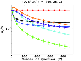
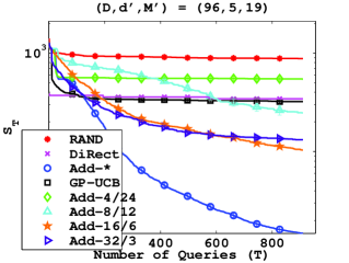
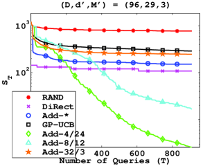
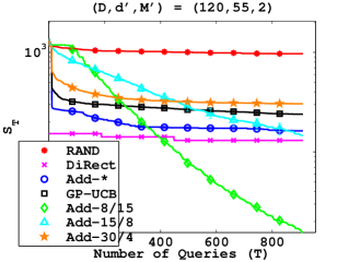
To demonstrate the efficacy of Add-GP-UCB over GP-UCB we optimise the acquisition function under a constrained budget. Following, Brochu et al. (2010) we use DiRect to maximise $\varphi_{t},\widetilde{\varphi}_{t}$. We compare Add-GP-UCB against GP-UCB, random querying (RAND) and DiRect. On the real datasets we also compare it to the Expected Improvement (GP-EI) acquisition function which is popular in BO applications and the method of Wang et al. (2013) which uses a random projection before applying BO (REMBO). We have multiple instantiations of Add-GP-UCB for different values for $(d,M)$. For optimisation, we perform comparisons based on the simple regret $S_{T}$ and for bandits we use the time averaged cumulative regret $R_{T}/T$.

For all GPB/ BO methods we set $N_{init}=10$, $N_{cyc}=25$ in all experiments. Further, for the first $25$ iterations we set the bandwidth to a small value $(10^{-5})$ to encourage an explorative strategy. We use SE kernels for each additive kernels and use the same scale $\sigma$ and bandwidth $h$ hyperparameters for all the kernels. Every $25$ iterations we maximise the marginal likelihood with respect to these $2$ hyperparameters in addition to the decomposition.

In contrast to existing literature in the BO community, we found that the UCB acquisitions outperformed GP-EI. One possible reason may be that under a constrained budget, UCB is robust to imperfect maximisation (Theorem 5) whereas GP-EI may not be. Another reason may be our choice of constants in UCB (Section 4.4).

Figure 3: Results on the synthetic datasets. In all images the $x$-axis is the number of queries and the $y$-axis is the regret in $\log$ scale. We have indexed each experiment by their $(D,{d^{\prime}},{M^{\prime}})$ values. The first row is $S_{T}$ for the experiments with $(D,{d^{\prime}},{M^{\prime}})$ set to $(10,3,3),(24,6,4),(24,11,2)$ and the second row is $R_{T}/T$ for the same experiments. The third row is $S_{T}$ for $(40,5,8),(40,18,2),(40,35,1)$ and the fourth row is the corresponding $R_{T}/T$. In some figures, the error bars are not visible since they are small and hidden by the bullets. All figures were produced by averaging over $20$ runs.

Figure 4: More results on synthetic experiments. The simple regret $S_{T}$ (first row) and cumulative regret $R_{T}/T$ (second row) for functions with $(D,{d^{\prime}},{M^{\prime}})$ set to $(96,5,19),(96,29,3),(120,55,2)$ respectively. Read the caption under Figure 3 for more details.

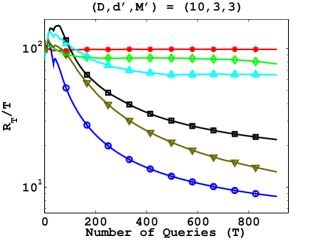
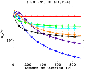
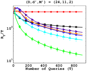
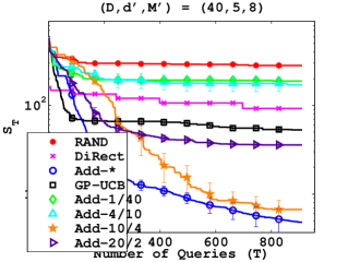
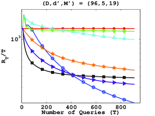
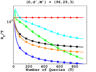
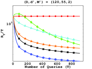
5.1 Simulations on Synthetic Data

First we demonstrate our technique on a series of synthetic examples. For this we construct additive functions for different values for the maximum group size ${d^{\prime}}$ and the number of groups ${M^{\prime}}$. We use the prime to distinguish it from Add-GP-UCB instantiations with different combinations of $(d,M)$ values. The ${d^{\prime}}$ dimensional function $f_{d^{\prime}}$ is,

$$f_{d^{\prime}}(x)=\log\Bigg{(}0.1\frac{1}{h_{d^{\prime}}^{d^{\prime}}}\exp\left(\frac{\|x-v_{1}\|^{2}}{2h_{d^{\prime}}^{2}}\right)+$$ (7)

$$\hskip 7.22743pt0.1\frac{1}{h_{d^{\prime}}^{d^{\prime}}}\exp\left(\frac{\|x-v_{2}\|^{2}}{2h_{d^{\prime}}^{2}}\right)+0.8\frac{1}{h_{d^{\prime}}^{d^{\prime}}}\exp\left(\frac{\|x-v_{3}\|^{2}}{2h_{d^{\prime}}^{2}}\right)\Bigg{)}$$

where $v_{1},v_{2},v_{3}$ are fixed ${d^{\prime}}$ dimensional vectors and $h_{d^{\prime}}=0.01{d^{\prime}}^{0.1}$. Then we create ${M^{\prime}}$ groups of coordinates by randomly adding ${d^{\prime}}$ coordinates into each group. On each such group we use $f_{d^{\prime}}$ and then add them up to obtain the composite function $f$. Precisely,

$$f(x)=f_{d^{\prime}}(x^{(1)})+\dots+f_{d^{\prime}}(x^{(M)})$$

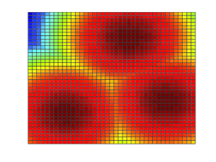
The remaining $D-{d^{\prime}}{M^{\prime}}$ coordinates do not contribute to the function. Since $f_{d^{\prime}}$ has $3$ modes, $f$ will have $3^{M^{\prime}}$ modes. We have illustrated $f_{d^{\prime}}$ for ${d^{\prime}}=2$ in Figure 2.

In the synthetic experiments we use an instantiation of Add-GP-UCB that knows the decomposition–i.e. $(d,M)=({d^{\prime}},{M^{\prime}})$ and the grouping of coordinates. We refer to this as Add-${\star}$. For the rest we use a $(d,M)$ decomposition by creating $M$ groups of size at most $d$ and find a good grouping by partially maximising the marginal likelihood (Section 4.4). We refer to them as Add-${d/M}$.

For GP-UCB we allocate a budget of $\min(5000,100D)$ DiRect function evaluations to optimise the acquisition function. For all Add-${d/M}$ methods we set it to $90\%$ of this amount to account for the additional overhead in posterior inference for each $f^{(j)}$. Therefore, in our $10D$ problem we maximise $\varphi_{t}$ with $\beta_{t}=2\log(2t)$ with $1000$ DiRect evaluations whereas for Add-${2/5}$ we maximise each $\widetilde{\varphi}_{t}^{(j)}$ with $\beta_{t}=0.4\log(2t)$ with $180$ evaluations.

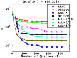
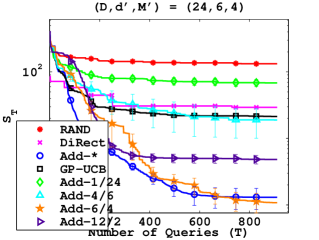
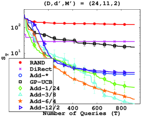
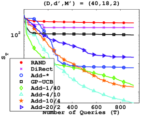
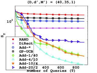
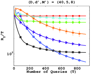
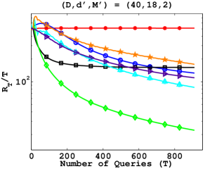
The results are given in Figures 3 and 4. We refer to each example by the configuration of the additive function–its $(D,{d^{\prime}},{M^{\prime}})$ values. In the $(10,3,3)$ example Add-${\star}$ does best since it knows the correct model and the acquisition function can be maximised within the budget. However Add-${3/4}$ and Add-${5/2}$ models do well too and outperform GP-UCB. Add-${1/10}$ performs poorly since it is statistically not expressive enough to capture the true function. In the $(24,11,2)$, $(40,18,2)$, $(40,35,1)$, $(96,29,3)$ and $(120,55,2)$ examples Add-${\star}$ outperforms GP-UCB. However, it is not competitive with the Add-${d/M}$ for small $d$. Even though Add-${\star}$ knew the correct decomposition, there are two possible failure modes since ${d^{\prime}}$ is large. The kernel is complex and the estimation error is very high in the absence of sufficient data points. In addition, optimising the acquisition is also difficult. This illustrates our previous argument that using an additive kernel can be advantageous even if the function is not additive or the decomposition is not known. In the $(24,6,4)$, $(40,5,8)$ and $(96,5,19)$ examples Add-${\star}$ performs best as ${d^{\prime}}$ is small enough. But again, almost all Add-${d/M}$ instantiations outperform GP-UCB. In contrast to the small $D$ examples, for large $D$, GP-UCB and Add-${d/M}$ with large $d$ perform worse than DiRect. This is probably because our budget for maximising $\varphi_{t}$ is inadequate to optimise the acquisition function to sufficient accuracy. For some of the large $D$ examples the cumulative regret is low for Add-GP-UCB and Add-${d/M}$ with large $d$. This is probably since they have already started exploiting where as the Add-${d/M}$ with small $d$ methods are still exploring. We posit that if we run for more iterations we will be able to see the improvements.

5.2 SDSS Astrophysical Dataset

Here we used Galaxy data from the Sloan Digital Sky Survey (SDSS). The task is to find the maximum likelihood estimators for a simulation based astrophysical likelihood model. Data and software for computing the likelihood are taken from Tegmark et al (2006). The software itself takes in only $9$ parameters but we augment this to $20$ dimensions to emulate the fact that in practical astrophysical problems we may not know the true parameters on which the problem is dependent. This also allows us to effectively demonstrate the superiority of our methods over alternatives. Each query to this likelihood function takes about 2-5 seconds. In order to be wall clock time competitive with RAND and DiRectwe use only $500$ evaluations for GP-UCB, GP-EI and REMBO and $450$ for Add-${d/M}$ to maximise the acquisition function.

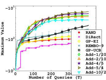
We have shown the Maximum value obtained over $400$ iterations of each algorithm in Figure 5. Note that RAND outperforms DiRect here since a random query strategy is effectively searching in $9$ dimensions. Despite this advantage to RAND all BO methods do better. Moreover, despite the fact that the function may not be additive, all Add-${d/M}$ methods outperform GP-UCB. Since the function only depends on $9$ parameters we use REMBO with a $9$ dimensional projection. Yet, it is not competitive with the Add-${d/M}$ methods. Possible reasons for this may include the scaling of the parameter space by $\sqrt{d}$ in REMBO and the imperfect optimisation of the acquisition function. Here Add-${5/4}$ performs slightly better than the rest since it seems to have the best tradeoff between being statistically expressive enough to capture the function while at the same time be easy enough to optimise the acquisition function within the allocated budget.

5.3 Viola & Jones Face Detection

The Viola & Jones (VJ) Cascade Classifier (Viola & Jones, 2001) is a popular method for face detection in computer vision based on the Adaboost algorithm. The $K$-cascade has $K$ weak classifiers which outputs a score for any given image. When we wish to classify an image we pass that image through each classifier. If at any point the score falls below a certain threshold the image is classified as negative. If the image passes through all classifiers then it is classified as positive. The threshold values at each stage are usually pre-set based on prior knowledge. There is no reason to believe that these threshold values are optimal. In this experiment we wish to find an optimal set of values for these thresholds by optimising the classification accuracy over a training set.

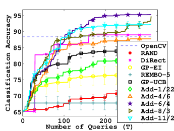
For this task, we use $1000$ images from the Viola & Jones face dataset containing both face and non-face images. We use the implementation of the VJ classifier that comes with OpenCV (Bradski & Kaehler, 2008) which uses a 22-stage cascade and modify it to take in the threshold values as a parameter. As our domain $\mathcal{X}$ we choose a neighbourhood around the configuration given in OpenCV. Each function call takes about 30-40 seconds and is the the dominant cost in this experiment. We use $1000$ DiRect evaluations to optimise the acquisition function for GP-UCB, GP-EI and REMBO and $900$ for the Add-${d/M}$ instantiations. Since we do not know the structure of the function we use REMBO with a $5$ dimensional projection. The results are given in Figure 5. Not surprisingly, REMBO performs worst as it is only searching on a $5$ dimensional space. Barring Add-${1/22}$ all other instantiations perform better than GP-UCB and GP-EI with Add-${6/4}$ performing the best. Interestingly, we also find a value for the thresholds that outperform the configuration used in OpenCV.

Figure 5: Results on the Astrophysical experiment 5 and the Viola and Jones dataset 5. The $x$-axis is the number of queries and the $y$-axis is the maximum value.

6 Conclusion

Recommendations: Based on our experiences, we recommend the following. If $f$ is known to be additive, the decomposition is known and $d$ is small enough so that $\widetilde{\varphi}_{t}$ can be efficiently optimised, then running Add-GP-UCB with the known decomposition is likely to produce the best results. If not, then use a small value for $d$ and run Add-GP-UCB while partially optimising for the decomposition periodically (Section 4.4). In our experiments we found that using $d$ between $3$ an $12$ seemed reasonable choices. However, note that this depends on the computational budget for optimising the acquisition, the query budget for $f$ and to a certain extent the the function $f$ itself.

Summary: Our algorithm takes into account several practical considerations in real world GPB/ BO applications such as computational constraints in optimising the acquisition and the fact that we have to work with a relatively few data points since function evaluations are expensive. Our framework effectively addresses these concerns without considerably compromising on the statistical integrity of the model. We believe that this provides a promising direction to scale GPB/ BO methods to high dimensions.

Future Work: Our experiments indicate that our methods perform well beyond the scope suggested by our theory. Developing an analysis that takes into account the bias-variance and computational tradeoffs in approximating and optimising a non-additive function via an additive model is an interesting challenge. We also intend to extend this framework to discrete settings, other acquisition functions and handle more general decompositions.

Appendix A Some Auxiliary Material

A.1 Review of the GP-UCB Algorithm

In this subsection we present a brief summary of the GP-UCB algorithm in (Srinivas et al., 2010). The algorithm is given in Algorithm 3.

The following theorem gives the rate of convergence for GP-UCB. Note that under an additive kernel, this is the same rate as Theorem 5 which uses a different acquisition function. Note the differences in the choice of $\beta_{t}$.

Theorem 6.

(Modification of Theorem 2 in (Srinivas et al., 2010)) Suppose $f$ is constructed by sampling $f^{(j)}\sim\mathcal{G}\mathcal{P}({\bf 0},\kappa^{(j)})$ for $j=1,\dots,M$ and then adding them. Let all kernels $\kappa^{(j)}$ satisfy assumption 2 for some $L,a,b$. Further, we maximise the acquisition function $\widetilde{\varphi}_{t}$ to within $\zeta_{0}t^{-1/2}$ accuracy at time step $t$. Pick $\delta\in(0,1)$ and choose

$$\beta_{t} =2\log\left(\frac{2t^{2}\pi^{2}}{\delta}\right)+2D\log\left(Dt^{3}\right)\;\;\in\;\mathcal{O}\left(D\log t\right).$$

Then, GP-UCB attains cumulative regret $R_{T}\in\mathcal{O}\left(\sqrt{\vphantom{T^{1}}D\gamma_{T}T\log T}\right)$ and hence simple regret $S_{T}\in\mathcal{O}\left(\sqrt{\vphantom{T^{1}}D\gamma_{T}\log T/T}\right)$. Precisely, with probability $>1-\delta$,

$$\forall T\geq 1,\;\;\;R_{T}\leq\sqrt{8C_{1}\beta_{T}MT\gamma_{t}}+2\zeta_{0}\sqrt{T}+C_{2}.$$

where $C_{1}=1/\log(1+\eta^{-2})$ and $C_{2}$ is a constant depending on $a$, $b$, $D$, $\delta$, $L$ and $\eta$.

Proof.

Srinivas et al. (2010) bound the regret for exact maximisation of the GP-UCB acquisition $\varphi_{t}$. By following an analysis similar to our proof of Theorem 5 the regret can be shown to be the same for an $\zeta_{0}t^{-1/2}$- optimal maximisation. ∎

Input: Kernel $\kappa$, Input Space $\mathcal{X}$.
For $t=1,2\dots$

• $\mathcal{D}_{0}\leftarrow\varnothing$,

• $(\mu_{0},\kappa_{0})\leftarrow({\bf 0},\kappa)$

• for $t=1,2,\dots$

  1. ${{\bf x}_{t}}\leftarrow\mathop{\mathrm{argmax}}_{z\in\mathcal{X}}\mu_{t-1}(z)+\sqrt{\beta_{t}}\sigma_{t-1}(z)$

  2. ${{\bf y}_{t}}\leftarrow\textrm{Query $f$ at ${{\bf x}_{t}}$}$.

  3. $\mathcal{D}_{t}=\mathcal{D}_{t-1}\cup\{({{\bf x}_{t}},{{\bf y}_{t}})\}$.

  4. Perform Bayesian posterior updates to obtain $\mu_{t},\sigma_{t}$ for $j=1,\dots,M$.

Algorithm 3 GP-UCB

A.2 Sequential Optimisation Approaches

If the function is known to be additive, we could consider several other approaches for maximisation. We list two of them here and explain their deficiencies. We recommend that the reader read the main text before reading this section.

A.2.1 Optimise one group and proceed to the next

First, fix the coordinates of $x^{(j)},j\neq 1$ and optimise w.r.t $x^{(1)}$ by querying the function for a pre-specified number of times. Then we proceed sequentially optimising with respect to $x^{(2)},x^{(3)}\dots$. We have outlined this algorithm in Algorithm 4. There are several reasons this approach is not desirable.

• First, it places too much faith on the additive assumption and requires that we know the decomposition at the start of the algorithm. Note that this strategy will only have searched the space in $M$ $d$-dimensional subspaces. In our approach even if the function is not additive we can still hope to do well since we learn the best additive approximation to the true function. Further, if the decomposition is not known we could learn the decomposition “on the go” or at least find a reasonably good decomposition as we have explained in Section 4.4.

• Such a sequential approach is not an anytime algorithm. This in particular means that we need to predetermine the number of queries to be allocated to each group. After we proceed to a new group it is not straightforward to come back and improve on the solution obtained for an older group.

• This approach is not suitable for the bandits setting. We suffer large instantaneous regret up until we get to the last group. Further, after we proceed beyond a group since we cannot come back, we cannot improve on the best regret obtained in that group.

Our approach does not have any of these deficiencies.

Input: Kernels $\kappa^{(1)},\dots,\kappa^{(M)}$, Decomposition $(\mathcal{X}^{(j)})_{j=1}^{M}$, Query Budget $T$,

• $\mathbb{R}^{D}\ni\theta=\bigcup_{j=1}^{M}\theta^{(j)}=\textrm{rand}([0,1]^{d})$

• for $j=1,\dots,M$

  1. $\mathcal{D}_{0}^{(j)}\leftarrow\varnothing$,

  2. $(\mu^{(j)}_{0},\kappa^{(j)}_{0})\leftarrow({\bf 0},\kappa^{(j)})$.

  3. for $t=1,2,\dots T/M$

     1. ${\bf x}_{t}^{(j)}\leftarrow\mathop{\mathrm{argmax}}_{z\in\mathcal{X}^{(j)}}\mu^{(j)}(z)+\sqrt{\beta_{t}}\sigma^{(j)}(z)$

     2. ${{\bf x}_{t}}\leftarrow{\bf x}_{t}^{(j)}\bigcup_{k\neq j}\theta^{(k)}$.

     3. ${{\bf y}_{t}}\leftarrow\textrm{Query $f$ at ${{\bf x}_{t}}$}$.

     4. $\mathcal{D}_{t}^{(j)}=\mathcal{D}_{t-1}^{(j)}\cup\{({\bf x}_{t}^{(j)},{{\bf y}_{t}})\}$.

     5. Perform Bayesian posterior updates to obtain $\mu^{(j)}_{t},\sigma^{(j)}_{t}$.

  4. $\theta^{(j)}\leftarrow{\bf x}^{(j)}_{T/M}$

• Return $\theta$

Algorithm 4 Seq-Add-GP-UCB

A.2.2 Only change one Group per Query

In this strategy, the approach would be very similar to Add-GP-UCB except that at each query we will only update one group at time. If it is the $k$${}^{\textrm{th}}$ group the query point is determined by maximising $\widetilde{\varphi}_{t}^{(k)}$ for ${\bf x}_{t}^{(k)}$ and for all other groups we use values from the previous rotation. After $M$ iterations we cycle through the groups. We have outlined this in Algorithm 5.

This is a reasonable approach and does not suffer from the same deficiencies as Algorithm 4. Maximising the acquisition function will also be slightly easier $\mathcal{O}(\zeta^{-d})$ since we need to optimise only one group at a time. However, the regret for this approach would be $\mathcal{O}(M\sqrt{\vphantom{T^{a}}D\gamma_{T}T\log T})$ which is a factor of $M$ worse than the regret in our method (This can be show by following an analysis similar to the one in section B.2. This is not surprising, since at each iteration you are moving in $d$-coordinates of the space and you have to wait $M$ iterations before the entire point is updated.

Input: Kernels $\kappa^{(1)},\dots,\kappa^{(M)}$, Decomposition $(\mathcal{X}^{(j)})_{j=1}^{M}$

• $\mathcal{D}_{0}\leftarrow\varnothing$,

• for $j=1,\dots,M$, $(\mu^{(j)}_{0},\kappa^{(j)}_{0})\leftarrow({\bf 0},\kappa^{(j)})$.

• for $t=1,2,\dots$

  1. $k=j\mod M$

  2. ${\bf x}_{t}^{(k)}\leftarrow\mathop{\mathrm{argmax}}_{z\in\mathcal{X}^{(k)}}\mu^{(k)}(z)+\sqrt{\beta_{t}}\sigma^{(k)}(z)$

  3. for $j\neq k$, ${\bf x}_{t}^{(j)}\leftarrow{\bf x}^{(j)}_{t-1}$

  4. ${{\bf x}_{t}}\leftarrow\bigcup_{j=1}^{M}{\bf x}_{t}^{(j)}$.

  5. ${{\bf y}_{t}}\leftarrow\textrm{Query $f$ at ${{\bf x}_{t}}$}$.

  6. $\mathcal{D}_{t}=\mathcal{D}_{t-1}\cup\{({{\bf x}_{t}},{{\bf y}_{t}})\}$.

  7. Perform Bayesian posterior updates to obtain $\mu^{(j)}_{t},\sigma^{(j)}_{t}$ for $j=1,\dots,M$.

Algorithm 5 Add-GP-UCB-Buggy

Appendix B Proofs of Results in Section 4.3

B.1 Bounding the Information Gain $\gamma_{T}$

For this we will use the following two results from Srinivas et al. (2010).

Lemma 7.

(Information Gain in GP, (Srinivas et al., 2010) Lemma 5.3) Using the basic properties of a GP, they show that

$$I(y_{A};f_{A})=\frac{1}{2}\sum_{t=1}^{n}\log(1+\eta^{-2}\sigma^{2}_{t-1}(x_{t})).$$

where $\sigma^{2}_{t-1}$ is the posterior variance after observing the first $t-1$ points.

Theorem 8.

(Bound on Information Gain, (Srinivas et al., 2010) Theorem 8) Suppose that $\mathcal{X}$ is compact and $\kappa$ is a kernel on $d$ dimensions satisfying Assumption 2. Let $n_{T}=C_{9}T^{\tau}\log T$ where $C_{9}=4d+2$. For any $T_{*}\in\{1,\dots,\min(T,n_{T})\}$, let $B_{\kappa}(T_{*})=\sum_{s>T_{*}}\lambda_{s}$. Here $(\lambda_{n})_{n\in\mathbb{N}}$ are the eigenvalues of $\kappa$ w.r.t the uniform distribution over $\mathcal{X}$. Then,

$$\gamma_{T}\leq\inf_{\tau}\left(\frac{1/2}{1-e^{-1}}\max_{r\in\left\{1,\dots,T\right\}}\left(T_{*}\log(rn_{T}/\eta^{2})+C_{9}\eta^{2}(1-r/T)(T^{\tau+1}B_{\kappa}(T_{*})+1)\log T\right)+\mathcal{O}(T^{1-\tau/d})\right).$$

B.1.1 Proof of Theorem 4-1

Proof.

We will use some bounds on the eigenvalues for the simple squared exponential kernel given in (Seeger et al., 2008). It was shown that the eigenvalues $\{\lambda^{(i)}_{s}\}$ of $\kappa^{(i)}$ satisfied $\lambda^{(i)}_{s}\leq c^{d}B^{s^{1/d_{i}}}$ where $B<1$ (See Remark 9). Since the kernel is additive, and $x^{(i)}\cap x^{(j)}=\varnothing$ the eigenfunctions corresponding to $\kappa^{(i)}$ and $\kappa^{(j)}$ will be orthogonal. Hence the eigenvalues of $\kappa$ will just be the union of the eigenvalues of the individual kernels – i.e. $\{\lambda_{s}\}=\bigcup_{j=1}^{M}\{\lambda^{(j)}_{s}\}$. As $B<1$, $\lambda^{(i)}_{s}\leq c^{d}B^{s^{1/d}}$. Let $T_{+}=\lfloor T_{*}/M\rfloor$ and $\alpha=-\log B$. Then,

$$B_{\kappa}(T_{*}) =\sum_{s>T_{*}}\lambda_{s}\leq Mc\sum_{s>T_{+}}B^{s^{1/d}}$$

$$\leq c^{d}M\left(B^{T_{+}^{1/d}}+\int_{T_{+}}^{\infty}\exp(-\alpha x^{1/d})\right)\mathrm{d}x$$

$$\leq c^{d}M\left(B^{T_{+}^{1/d}}+d\alpha^{-d}\Gamma(d,\alpha T_{+}^{1/d})\right)$$

$$\leq c^{d}Me^{-\alpha T_{+}^{1/d}}\left(1+d!d\alpha^{-d}(\alpha T_{+}^{1/d})^{d-1}\right).$$

The last step holds true whenever $\alpha T_{+}^{1/d}\geq 1$. Here in the second step we bound the series by an integral and in the third step we used the substitution $y=\alpha x^{1/d}$ to simplify the integral. Here $\Gamma(s,x)=\int_{x}^{\infty}t^{s-1}e^{-t}\mathrm{d}t$ is the (upper) incomplete Gamma function. In the last step we have used the following identity and the bound for integral $s$ and $x\geq 1$

$$\Gamma(s,x)=(s-1)!e^{-x}\sum_{k=0}^{s-1}\frac{x^{k}}{k!}\leq s!e^{-x}x^{d-1}.$$

By using $\tau=d$ and by using $T_{*}\leq(M+1)T_{+}$, we use Theorem 8 to obtain the following bound on $\gamma_{T}$,

$$\gamma_{T} \leq\frac{1/2}{1-e^{-1}}\max_{r\in\left\{1,\dots,T\right\}}\bigg{(}(M+1)T_{+}\log(rn_{T}/\eta^{2})+$$

$$\hskip 14.45377ptC_{9}\eta^{2}(1-r/T)\log T\left(1+c^{d}Me^{-\alpha T_{+}^{1/d}}T^{d+1}\left(1+d!d\alpha^{-d}(\alpha T_{+}^{1/d})^{d-1}\right)\right)\bigg{)}.$$ (8)

Now we need to pick $T_{+}$ so as to balance these two terms. We will choose $T_{+}=\left(\frac{\log(Tn_{T})}{\alpha}\right)^{d}$ which is less than $\min(T,n_{T})/M$ for sufficiently large $T$. Then $e^{-\alpha T_{+}^{1/d}}=1/Tn_{T}$. Then the first term $S_{1}$ inside the paranthesis is,

$$S_{1}=(M+1)\log^{d}\left(\frac{Tn_{T}}{\alpha}\right)\log\left(\frac{rn_{T}}{\eta^{2}}\right) \in\mathcal{O}\left(M\left(\log(Tn_{T})\right)^{d}\log(rn_{T})\right)$$

$$\in\mathcal{O}\left(M\left(\log(T^{d+1}\log T)\right)^{d}\log(rT^{d}\log T)\right)$$

$$\in\mathcal{O}\left(Md^{d+1}(\log T)^{d+1}+Md^{d}(\log T)^{d}\log(r)\right).$$

Note that the constant in front has exponential dependence on $d$ but we ignore it since we already have $d^{d}$, $(\log T)^{d}$ terms. The second term $S_{2}$ becomes,

$$S_{2} =C_{9}\eta^{2}(1-r/T)\log T\left(1+\frac{c^{d}M}{Tn_{T}}T^{d+1}\left(1+d!d\alpha^{-d}(\log(Tn_{T})^{d-1}\right)\right)\bigg{)}$$

$$\leq C_{9}\eta^{2}(1-r/T)\left(\log T+\frac{c^{d}M}{C_{9}}\left(1+d!d\alpha^{-d}(\log(Tn_{T})^{d-1}\right)\right)\bigg{)}$$

$$\leq C_{9}\eta^{2}(1-r/T)\left(\mathcal{O}(\log T)+\mathcal{O}(1)+\mathcal{O}(d!d^{d}(\log T)^{d-1})\right)\bigg{)}$$

$$\in\mathcal{O}\left((1-r/T)d!d^{d}(\log T)^{d-1}\right).$$

Since $S_{1}$ dominates $S_{2}$, we should choose $r=T$ to maximise the RHS in (8). This gives us,

$$\gamma_{T}\;\in\;\mathcal{O}\left(Md^{d+1}(\log T)^{d+1}\right)\;\in\;\mathcal{O}\left(Dd^{d}(\log T)^{d+1}\right).$$

∎

B.1.2 Proof of Theorem 4-2

Proof.

Once again, we use bounds given in (Seeger et al., 2008). It was shown that the eigenvalues $\{\lambda^{(i)}_{s}\}$ for $\kappa^{(i)}$ satisfied $\lambda^{(i)}_{s}\leq c^{d}s^{-\frac{2\nu+d_{j}}{d_{j}}}$ (See Remark 9). By following a similar argument to above we have $\{\lambda_{s}\}=\bigcup_{j=1}^{M}\{\lambda^{(j)}_{s}\}$ and $\lambda^{(i)}_{s}\leq c^{d}s^{-\frac{2\nu+d}{d}}$. Let $T_{+}=\lfloor T_{*}/M\rfloor$. Then,

$$B_{\kappa}(T_{*})=\sum_{s>T_{*}}\lambda_{s}\leq Mc^{d}\sum_{s>T_{+}}s^{-\frac{2\nu+d}{d}}\leq Mc^{d}\left(T_{+}^{-\frac{2\nu+d}{d}}+\int_{T_{+}}^{\infty}s^{-\frac{2\nu+d}{d}}\right)\leq C_{8}2^{d}MT_{+}^{1-\frac{2\nu+d}{d}}.$$

where $C_{8}$ is an appropriate constant. We set $T_{+}=(Tn_{T})^{\frac{d}{2\nu+d}}(\log(Tn_{T}))^{-\frac{d}{2\nu+d}}$ and accordingly we have the following bound on $\gamma_{T}$ as a function of $T_{+}\in\{1,\dots,\min(T,n_{T})/M\}$,

$$\gamma_{T}\leq\inf_{\tau}\Bigg{(}\frac{1/2}{1-e^{-1}}\max_{r\in\left\{1,\dots,T\right\}}\bigg{(}(M+1)T_{+}\log(rn_{T}/\eta^{2})+C_{9}\eta^{2}(1-r/T)\left(\log T+C_{8}2^{d}MT_{+}\log(Tn_{T})\right)\bigg{)}+\mathcal{O}(T^{1-\tau/d})\Bigg{)}.$$ (9)

Since this is a concave function on $r$ we can find the optimum by setting the derivative w.r.t $r$ to be zero. We get $r\in\mathcal{O}(T/2^{d}\log(Tn_{T}))$ and hence,

$$\gamma_{T} \in\inf_{\tau}\left(\mathcal{O}\left(MT_{+}\log\left(\frac{Tn_{T}}{2^{d}\log(Tn_{T})}\right)\right)+\mathcal{O}\left(M2^{d}T_{+}\log(Tn_{T})\right)+\mathcal{O}(T^{1-\tau/d})\right)$$

$$\in\inf_{\tau}\left(\mathcal{O}\left(M2^{d}\log(Tn_{T})\left(\frac{T^{\tau+1}\log(T)}{(\tau+1)\log(T)+\log\log T}\right)^{\frac{d}{2\nu+d}}\right)+\mathcal{O}(T^{1-\tau/d})\right)$$

$$\in\inf_{\tau}\left(\mathcal{O}\left(M2^{d}\log(Tn_{T})T^{\frac{(\tau+1)d}{2\nu+d}}\right)+\mathcal{O}(T^{1-\tau/d})\right)$$

$$\in\mathcal{O}\left(M2^{d}T^{\frac{d(d+1)}{2\nu+d(d+1)}}\log(T)\right).$$

Here in the second step we have substituted the values for $T_{+}$ first and then $n_{T}$. In the last step we have balanced the polynomial dependence on $T$ in both terms by setting $\tau=\frac{2\nu d}{2\nu+d(d+1)}$.
∎

Remark 9.

The eigenvalues and eigenfunctions for the kernel are defined with respect to a base distribution on $\mathcal{X}$. In the development of Theorem 8, Srinivas et al. (2010) draw $n_{T}$ samples from the uniform distribution on $\mathcal{X}$. Hence, the eigenvalues/eigenfunctions should be w.r.t the uniform distribution. The bounds given in Seeger et al. (2008) are for the uniform distribution for the Matérn kernel and a Gaussian Distribution for the Squared Exponential Kernel. For the latter case, Srinivas et al. (2010) argue that the uniform distribution still satisfies the required tail constraints and therefore the bounds would only differ up to constants.

B.2 Rates on Add-GP-UCB

Our analysis in this section draws ideas from Srinivas et al. (2010). We will try our best to stick to their same notation. However, unlike them we also handle the case where the acquisition function is optimised within some error. In the ensuing discussion, we will use ${{\bf\tilde{x}}_{t}}=\bigcup_{j}{\bf\tilde{x}}_{t}^{(j)}$ to denote the true maximiser of $\widetilde{\varphi}_{t}$ – i.e. ${\bf\tilde{x}}_{t}^{(j)}=\mathop{\mathrm{argmax}}_{z\in\mathcal{X}^{(j)}}\widetilde{\varphi}_{t}^{(j)}(z)$. ${{\bf x}_{t}}=\bigcup_{j}{\bf x}_{t}^{(j)}$ denotes the point chosen by Add-GP-UCB at the $t^{th}$ iteration. Recall that ${{\bf x}_{t}}$ is $\zeta_{0}t^{-1/2}$–optimal; I.e. $\widetilde{\varphi}_{t}({{\bf\tilde{x}}_{t}})-\widetilde{\varphi}_{t}({{\bf x}_{t}})\leq\zeta_{0}t^{-1/2}$.

Denote $p=\sum_{j}d_{j}$. $\pi_{t}$ denotes a sequence such that $\sum_{t}\pi_{t}^{-1}=1$. For e.g. when we use $\pi_{t}=\pi^{2}t^{2}/6$ below, we obtain the rates in Theorem 5.

In what follows, we will construct discretisations $\Omega^{(j)}$ on each group $\mathcal{X}^{(j)}$ for the sake of analysis. Let $\omega_{j}=|\Omega^{(j)}|$ and $\omega_{m}=\max_{j}\omega_{j}$. The discretisation of the individual groups induces a discretisation $\Omega$ on $\mathcal{X}$ itself, $\Omega=\{\rm=\bigcup_{j}{\bf x}^{(j)}:{\bf x}^{(j)}\in\Omega^{(j)},j=1,\dots,M\}$. Let $\omega=|\Omega|=\prod_{j}\omega_{j}$. We first establish the following two lemmas before we prove Theorem 5.

Lemma 10.

Pick $\delta\in(0,1)$ and set $\beta_{t}=2\log(\omega_{m}M\pi_{t}/\delta)$. Then with probability $>1-\delta$,

$$\forall t\geq 1,\forall\rm\in\Omega,\hskip 14.45377pt|f(\rm)-\mu_{t-1}(\rm)|\leq\beta_{t}^{1/2}\sum_{j=1}^{M}\sigma^{(j)}_{t-1}({\bf x}^{(j)}).$$

Proof.

Conditioned on $\mathcal{D}_{t-1}$, at any given and $t$ we have $f({\bf x}^{(j)})\sim\mathcal{N}(\mu^{(j)}_{t-1}({\bf x}^{(j)}),\sigma^{(j)}_{t-1}{j}),\;\forall j=1,\dots M$. Using the tail bound, $\mathbb{P}(z>M)\leq\frac{1}{2}e^{-M^{2}/2}$ for $z\sim\mathcal{N}(0,1)$ we have with probability $>1-\delta/\omega M\pi_{t}$,

$$\frac{|f^{(j)}({\bf x}^{(j)})-\mu^{(j)}_{t-1}({\bf x}^{(j)})|}{\sigma^{(j)}_{t-1}({\bf x}^{(j)})}>\beta_{t}^{1/2}\leq e^{-\beta_{t}/2}=\frac{\delta}{\omega_{m}M\pi_{t}}.$$

By using a union bound $\omega_{j}\leq\omega_{m}$ times over all ${\bf x}^{(j)}\in\Omega^{(j)}$ and then $M$ times over all discretisations the above holds with probability $>1-\delta/\pi_{t}$ for all $j=1,\dots,M$ and ${\bf x}^{(j)}\in\Omega^{(j)}$. Therefore, we have $|f(\rm)-\mu_{t-1}(\rm)|\leq|f({\bf x}^{(j)})-\mu^{(j)}_{t-1}({\bf x}^{(j)})|\leq\beta_{t}^{1/2}\sum_{j}\sigma^{(j)}_{t-1}({\bf x}^{(j)})$ for all $\rm\in\Omega$. Now using the union bound on all $t$ yields the result.
∎

Lemma 11.

The posterior mean $\mu_{t-1}$ for a GP whose kernel $\kappa(\cdot,x)$ is $L$-Lipschitz satisfies,

$$\mathbb{P}\left(\forall t\geq 1\;\;\;|\mu_{t-1}(x)-\mu_{t-1}(x^{\prime})|\leq\left(f(\rm_{*})+\eta\sqrt{2\log(\pi_{t}/2\delta)}\right)L\eta^{-2}t\|x-x^{\prime}\|_{2}\right)\geq 1-\delta.$$

Proof.

Note that for given $t$,

$$\mathbb{P}\left(y_{t}<f(\rm_{*})+\eta\sqrt{2\log(\pi_{t}/2\delta)}\right)\leq\mathbb{P}\left(\epsilon_{t}/\eta<\sqrt{2\log(\pi_{t}/2\delta)}\right)\leq\delta/\pi_{t}.$$

Therefore the statement is true with probability $>1-\delta$ for all $t$. Further, $\Delta\succ\eta^{2}I$ implies $\|\Delta^{-1}\|_{op}\leq\eta^{-2}$ and $|k(x,z)-k(x^{\prime},z)|\leq L\|x-x^{\prime}\|$. Therefore

$$|\mu_{t-1}(x)-\mu_{t-1}(x^{\prime})|=|Y_{t-1}^{\top}\Delta^{-1}(k(x,X_{T})-k(x^{\prime},X_{T})|\leq\|Y_{t-1}\|_{2}\|\Delta^{-1}\|_{op}\|k(x,X_{t-1})-k(x^{\prime},X_{t-1})\|_{2}$$

$$\hskip 14.45377pt\leq\left(f(\rm_{*})+\eta\sqrt{2\log(\pi_{t}/2\delta)}\right)L\eta^{-2}(t-1)\|x-x^{\prime}\|_{2}.$$

∎

B.2.1 Proof of Theorem 5

Proof.

First note that by Assumption 2 and the union bound we have, $\mathbb{P}(\forall i\;\sup_{x^{(j)}\in\mathcal{X}^{(j)}}|{\partial f^{(j)}(x^{(j)})}/{\partial x^{(j)}_{i}}|>J)\leq d_{i}ae^{-(J/b)^{2}}$. Since, ${\partial f(x)}/{\partial x^{(j)}_{i}}={\partial f^{(j)}(x^{(j)})}/{\partial x^{(j)}_{i}}$, we have,

$$\mathbb{P}\left(\forall i=1,\dots,D\;\sup_{x\in\mathcal{X}}\Big{|}\frac{\partial f(x)}{\partial x_{i}}\Big{|}>J\right)\leq pae^{-(J/b)^{2}}.$$

By setting $\delta/3=pae^{-J^{2}/b^{2}}$ we have with probability $>1-\delta/3$,

$$\forall x,x^{\prime}\in\mathcal{X},\;|f(x)-f(x^{\prime})|\leq b\sqrt{\log(3ap/\delta)}\|x-x^{\prime}\|_{1}.$$ (10)

Now, we construct a sequence of discretisations $\Omega^{(j)}_{t}$ satisfying $\|x^{(j)}-[x^{(j)}]_{t}]\|_{1}\leq d_{j}/\tau_{t}\;\;\forall x^{(j)}\in\Omega^{(j)}_{t}$. Here, $[x^{(j)}]_{t}$ is the closest point to $x^{(j)}$ in $\Omega^{(j)}_{t}$ in an $L_{2}$ sense. A sufficient discretisation is a grid with $\tau_{t}$ uniformly spaced points. Then it follows that for all $x\in\Omega_{t}$, $\|x-[x]_{t}\|_{1}\leq p/\tau_{t}$. Here $\Omega_{t}$ is the discretisation induced on $\mathcal{X}$ by the $\Omega^{(j)}_{t}$’s and $[x]_{t}$ is the closest point to $x$ in $\Omega_{t}$. Note that $\|x^{(j)}-[x^{(j)}]_{t}\|_{2}\leq\sqrt{d_{j}}/\tau_{t}\;\forall x^{(j)}\in\Omega^{(j)}$ and $\|x-[x]_{t}\|_{2}\leq\sqrt{p}/\tau_{t}$. We will set $\tau_{t}=pt^{3}$–therefore, $\omega_{tj}\leq(pt^{3})^{d}\stackrel{{\scriptstyle\Delta}}{{=}}\omega_{mt}$. When combining this with (10), we get that with probability $>1-\delta/3$, $|f(x)-f([x])|\leq b\sqrt{\log(3ap/\delta)}/t^{3}$. By our choice of $\beta_{t}$ and using Lemma 10 the following is true for all $t\geq 1$ and for all $x\in\mathcal{X}$ with probability $>1-2\delta/3$,

$$|f(x)-\mu_{t-1}([x]_{t})|\leq|f(x)-f([x]_{t})|+|f([x]_{t})-\mu_{t-1}([x]_{t})|\leq\frac{b\sqrt{\log(3ap/\delta)}}{t^{2}}+\beta_{t}^{1/2}\sum_{j=1}^{M}\sigma^{(j)}_{t-1}([x^{(j)}]_{t}).$$ (11)

By Lemma 11 with probability $>1-\delta/3$ we have,

$$\forall x\in\mathcal{X},\;\;\;|\mu_{t-1}(x)-\mu_{t-1}([x]_{t})|\leq\frac{L\left(f(\rm_{*})+\eta\sqrt{2\log(3\pi_{t}/2\delta)}\right)}{\sqrt{p}\eta^{2}t^{2}}.$$ (12)

We use the above results to obtain the following bound on the instantaneous regret $r_{t}$ which holds with probability $>1-\delta$ for all $t\geq 1$,

$$r_{t} =f(\rm_{*})-f({{\bf x}_{t}})$$

$$\leq\mu_{t-1}([\rm_{*}]_{t})+\beta_{t}^{1/2}\sum_{j=1}^{M}\sigma^{(j)}_{t-1}([\rm_{*}^{(j)}]_{t})-\mu_{t-1}([{{\bf x}_{t}}]_{t})+\beta_{t}^{1/2}\sum_{j=1}^{M}\sigma^{(j)}_{t-1}([{\bf x}_{t}^{(j)}]_{t})+\frac{2b\sqrt{\log(3ap/\delta)}}{t^{3}}$$

$$\leq\frac{2b\sqrt{\log(3ap/\delta)}}{t^{3}}+\frac{\zeta_{0}}{\sqrt{t}}+\beta_{t}^{1/2}\left(\sum_{j=1}^{M}\sigma^{(j)}_{t-1}({\bf x}_{t}^{(j)})+\sum_{j=1}^{M}\sigma^{(j)}_{t-1}([{\bf x}_{t}^{(j)}]_{t})\right)+\mu_{t-1}({{\bf x}_{t}})-\mu_{t-1}([{{\bf x}_{t}}]_{t})$$

$$\leq\frac{2b\sqrt{\log(3ap/\delta)}}{t^{3}}+\frac{L\left(f(\rm_{*})+\eta\sqrt{2\log(\pi_{t}/2\delta)}\right)}{\sqrt{p}\eta^{2}t^{2}}+\frac{\zeta_{0}}{\sqrt{t}}+\beta_{t}^{1/2}\left(\sum_{j=1}^{M}\sigma^{(j)}_{t-1}({\bf x}_{t}^{(j)})+\sum_{j=1}^{M}\sigma^{(j)}_{t-1}([{\bf x}_{t}^{(j)}]_{t})\right).$$ (13)

In the first step we have applied Equation (11) at _∗ and ${{\bf x}_{t}}$. In the second step we have used the fact that $\widetilde{\varphi}_{t}([\rm_{*}]_{t})\leq\widetilde{\varphi}_{t}({{\bf\tilde{x}}_{t}})\leq\widetilde{\varphi}_{t}({{\bf x}_{t}})+\zeta_{0}t^{-1/2}$. In the third step we have used Equation (12).

For any $x\in\mathcal{X}$ we can bound ${\sigma_{t}(x)}^{2}$ as follows,

$${\sigma_{t}(x)}^{2}=\eta^{2}\eta^{-2}{\sigma_{t}(x)}^{2}\leq\frac{1}{\log(1+\eta^{-2})}\log\left(1+\eta^{-2}{\sigma_{t}(x)}^{2}\right).$$

Here we have used the fact that $u^{2}\leq v^{2}\log(1+u^{2})/\log(1+v^{2})$ for $u\leq v$ and ${\sigma_{t}(\rm)}^{2}\leq\kappa(x,x)=1$. Write $C_{1}=\log^{-1}(1+\eta^{-2})$. By using Jensen’s inequality and Definition 3 for any set of $T$ points $\{x_{1},x_{2},\dots x_{T}\}\subset\mathcal{X}$,

$$\left(\sum_{t=1}^{T}\sum_{j=1}^{M}\sigma^{(j)}_{t}(x^{(j)})\right)^{2}\leq MT\sum_{t=1}^{T}\sum_{j=1}^{M}{\sigma^{(j)}_{t}(x^{(j)})}^{2}\leq C_{1}MT\sum_{t=1}^{T}\log\left(1+\eta^{-2}{\sigma_{t}(x)}^{2}\right)\leq 2C_{1}MT\gamma_{T}.$$ (14)

Finally we can bound the cumulative regret with probability $>1-\delta$ for all $T\geq 1$ by,

$$R_{T} =\sum_{t=1}^{T}r_{t}\leq C_{2}(a,b,D,L,\delta)+\zeta_{0}\sum_{t=1}^{T}t^{-1/2}+\beta_{T}^{1/2}\left(\sum_{t=1}^{T}\sum_{j=1}^{M}\sigma^{(j)}_{t-1}({\bf x}_{t}^{(j)})+\sum_{t=1}^{T}\sum_{j=1}^{M}\sigma^{(j)}_{t-1}([{\bf x}_{t}^{(j)}]_{t})\right)$$

$$\leq C_{2}(a,b,D,L,\delta)+2\zeta_{0}\sqrt{T}+\sqrt{8C_{1}\beta_{T}MT\gamma_{T}}.$$

where we have used the summability of the first two terms in Equation (13). Here, for $\delta<0.8$, the constant $C_{2}$ is given by,

$$C_{2}\geq b\sqrt{\log(3ap/\delta)}+\frac{\pi^{2}Lf(\rm_{*})}{6\sqrt{p}\eta^{2}}+\frac{L\pi^{3/2}}{\sqrt{12p\delta}\eta}.$$

∎

References

- Auer (2003) Auer, Peter. Using Confidence Bounds for Exploitation-exploration Trade-offs. J. Mach. Learn. Res., 2003.
- Azimi et al. (2010) Azimi, Javad, Fern, Alan, and Fern, Xiaoli Z. Batch Bayesian Optimization via Simulation Matching. In Advances in Neural Information Processing Systems, 2010.
- Bergstra et al. (2011) Bergstra, James S., Bardenet, Rémi, Bengio, Yoshua, and Kégl, Balázs. Algorithms for Hyper-Parameter Optimization. In Advances in Neural Information Processing Systems, 2011.
- Bradski & Kaehler (2008) Bradski, Gary and Kaehler, Adrian. Learning OpenCV. O’Reilly Media Inc., 2008.
- Brochu et al. (2010) Brochu, Eric, Cora, Vlad M., and de Freitas, Nando. A Tutorial on Bayesian Optimization of Expensive Cost Functions, with Application to Active User Modeling and Hierarchical Reinforcement Learning. CoRR, 2010.
- Bull (2011) Bull, Adam D. Convergence Rates of Efficient Global Optimization Algorithms. Journal of Machine Learning Research, 2011.
- Chen et al. (2012) Chen, Bo, Castro, Rui, and Krause, Andreas. Joint Optimization and Variable Selection of High-dimensional Gaussian Processes. In Int’l Conference on Machine Learning, 2012.
- de Freitas (2014) de Freitas, Nando. Talk on Current Challenges and Open Problems in Bayesian Optimization, 2014.
- de Freitas et al. (2012) de Freitas, Nando, Smola, Alex J., and Zoghi, Masrour. Exponential Regret Bounds for Gaussian Process Bandits with Deterministic Observations. In International Conference on Machine Learning, 2012.
- Denil et al. (2012) Denil, Misha, Bazzani, Loris, Larochelle, Hugo, and de Freitas, Nando. Learning Where to Attend with Deep Architectures for Image Tracking. Neural Comput., 2012.
- Djolonga et al. (2013) Djolonga, Josip, Krause, Andreas, and Cevher, Volkan. High-Dimensional Gaussian Process Bandits. In Advances in Neural Information Processing Systems, 2013.
- Duvenaud et al. (2011) Duvenaud, David K., Nickisch, Hannes, and Rasmussen, Carl Edward. Additive gaussian processes. In Advances in Neural Information Processing Systems, 2011.
- Ghosal & Roy (2006) Ghosal, Subhashis and Roy, Anindya. Posterior consistency of Gaussian process prior for nonparametric binary regression”. Annals of Statistics, 2006.
- Gonzalez et al. (2014) Gonzalez, Javier, Longworth, Joseph, James, David, and Lawrence, Neil. Bayesian Optimization for Synthetic Gene Design. In NIPS Workshop on Bayesian Optimization in Academia and Industry, 2014.
- Györfi et al. (2002) Györfi, László, Kohler, Micael, Krzyzak, Adam, and Walk, Harro. A Distribution Free Theory of Nonparametric Regression. Springer Series in Statistics, 2002.
- Hastie & Tibshirani (1990) Hastie, T. J. and Tibshirani, R. J. Generalized Additive Models. London: Chapman & Hall, 1990.
- Hoffman et al. (2011) Hoffman, Matthew D., Brochu, Eric, and de Freitas, Nando. Portfolio Allocation for Bayesian Optimization. In Uncertainty in Artificial Intelligence, 2011.
- Hornby et al. (2006) Hornby, G. S., Globus, A., Linden, D.S., and Lohn, J.D. Automated Antenna Design with Evolutionary Algorithms. American Institute of Aeronautics and Astronautics, 2006.
- Jones et al. (1993) Jones, D. R., Perttunen, C. D., and Stuckman, B. E. Lipschitzian Optimization Without the Lipschitz Constant. J. Optim. Theory Appl., 1993.
- Jones et al. (1998) Jones, Donald R., Schonlau, Matthias, and Welch, William J. Efficient global optimization of expensive black-box functions. J. of Global Optimization, 1998.
- Kandasamy et al. (2015) Kandasamy, Kirthevasan, Schneider, Jeff, and Póczos, Barnabás. Bayesian Active Learning for Posterior Estimation. In International Joint Conference on Artificial Intelligence, 2015.
- Lizotte et al. (2007) Lizotte, Daniel, Wang, Tao, Bowling, Michael, and Schuurmans, Dale. Automatic gait optimization with gaussian process regression. In in Proc. of IJCAI, pp. 944–949, 2007.
- Ma et al. (2015) Ma, Yifei, Sutherland, Dougal J., Garnett, Roman, and Schneider, Jeff G. Active Pointillistic Pattern Search. In International Conference on Artificial Intelligence and Statistics, AISTATS, 2015.
- Mahendran et al. (2012) Mahendran, Nimalan, Wang, Ziyu, Hamze, Firas, and de Freitas, Nando. Adaptive MCMC with Bayesian Optimization. In Artificial Intelligence and Statistics, 2012.
- Martinez-Cantin et al. (2007) Martinez-Cantin, R., de Freitas, N., Doucet, A., and Castellanos, J. Active Policy Learning for Robot Planning and Exploration under Uncertainty. In Proceedings of Robotics: Science and Systems, 2007.
- Mockus & Mockus (1991) Mockus, J.B. and Mockus, L.J. Bayesian approach to global optimization and application to multiobjective and constrained problems. Journal of Optimization Theory and Applications, 1991.
- Mockus (1994) Mockus, Jonas. Application of Bayesian approach to numerical methods of global and stochastic optimization. Journal of Global Optimization, 1994.
- Osborne et al. (2012) Osborne, M., Duvenaud, D., Garnett, R., Rasmussen, C., Roberts, S., and Ghahramani, Z. Active Learning of Model Evidence Using Bayesian Quadrature. In Neural Information Processing Systems (NIPS), 2012.
- Parkinson et al. (2006) Parkinson, David, Mukherjee, Pia, and Liddle, Andrew R. A Bayesian model selection analysis of WMAP3. Physical Review, 2006.
- Rasmussen & Williams (2006) Rasmussen, C.E. and Williams, C.K.I. Gaussian Processes for Machine Learning. Adaptative computation and machine learning series. University Press Group Limited, 2006.
- Ravikumar et al. (2009) Ravikumar, Pradeep, Lafferty, John, Liu, Han, and Wasserman, Larry. Sparse Additive Models. Journal of the Royal Statistical Society: Series B (Statistical Methodology), 2009.
- Seeger et al. (2008) Seeger, MW., Kakade, SM., and Foster, DP. Information Consistency of Nonparametric Gaussian Process Methods. IEEE Transactions on Information Theory, 2008.
- Snoek et al. (2012) Snoek, Jasper, Larochelle, Hugo, and Adams, Ryan P. Practical Bayesian Optimization of Machine Learning Algorithms. In Advances in Neural Information Processing Systems, 2012.
- Srinivas et al. (2010) Srinivas, Niranjan, Krause, Andreas, Kakade, Sham, and Seeger, Matthias. Gaussian Process Optimization in the Bandit Setting: No Regret and Experimental Design. In International Conference on Machine Learning, 2010.
- Tegmark et al (2006) Tegmark et al, M. Cosmological Constraints from the SDSS Luminous Red Galaxies. Physical Review, December 2006.
- Thompson (1933) Thompson, W. R. On the Likelihood that one Unknown Probability Exceeds Another in View of the Evidence of Two Samples. Biometrika, 1933.
- Viola & Jones (2001) Viola, Paul A. and Jones, Michael J. Rapid Object Detection using a Boosted Cascade of Simple Features. In Computer Vision and Pattern Recognition, 2001.
- Wang et al. (2013) Wang, Ziyu, Zoghi, Masrour, Hutter, Frank, Matheson, David, and de Freitas, Nando. Bayesian Optimization in High Dimensions via Random Embeddings. In International Joint Conference on Artificial Intelligence, 2013.
- Yamins et al. (2013) Yamins, Daniel, Tax, David, and Bergstra, James S. Making a Science of Model Search: Hyperparameter Optimization in Hundreds of Dimensions for Vision Architectures. In International Conference on Machine Learning, 2013.