Abstract

We show that for 1+1 dimensional Causal Dynamical Triangulations (CDT) coupled to 4 massive scalar fields one can construct an effective transfer matrix if the masses squared is larger than or equal to 0.05. The properties of this transfer matrix can explain why CDT coupled to matter can behave completely different from “pure” CDT. We identify the important critical exponent in the effective action, which may determine the universality class of the model.

1 Introduction

Causal Dynamical Triangulations (CDT) in 1+1 dimensions can be considered a toy model for more advanced models of quantum gravity. The simplest version of the model, pure fluctuating geometry without matter, can be solved analytically [2]. The random geometries present in the CDT path integral are constructed by gluing together flat simplices (triangles) in such a way that one has a global time foliation. The topology of space at a given time is assumed to be $S^{1}$. This topology is preserved in the time evolution. In all our considerations time is Wick rotated and the triangles used are assumed to be equilateral with edge lengths $a$. We label time with integer numbers $t$. The geometry of a spatial slice at time $t$ is completely characterized by its length, i.e. in the CDT model by $n(t)$ - the number of edges forming the spatial $S^{1}$ . In the path integral representation of the time evolution, spatial states at integer times $t$ and $t+1$ are connected in all possible ways consistent with the foliation. In the case of CDT without matter fields the time evolution is generated by a transfer matrix $\langle n_{t}|{\cal M}|n_{t+1}\rangle=\exp(-L(n_{t},n_{t+1}))$ with correctly normalized spatial states $|n\rangle$. The explicit expression for $L(n,m)$ can be interpreted as a term of the effective action, since in obtaining it we sum over all geometrical realizations joining the two states.

One may view the same geometry using a dual trivalent lattice, where vertices are located in the centers of triangles and links being dual to the edges in the original lattice. Each vertex has exactly three neighbors, two at the same time $t$ (which can be considered as a half-integer time with respect to the original triangulation) and one at time $t\pm 1$. As before the links at the same time value form a closed spatial geometry $S^{1}$, the quantities $n_{t}$ and $n_{t+1}$ represent numbers of links pointing up or down from the line at $t+1/2$. The dual formulation is completely equivalent to the original one and we will use it in this article.

The Hilbert-Einstein action for a triangulation ${\cal T}$, $S({\cal T})$, provides the weight $\exp(-S({\cal T}))$ to be assigned to the triangulation in the path integral. In 1+1 dimensions there is no curvature term (it is a topological invariant), and we are left with the cosmological term, which on the lattice takes to form

$$S({\cal T})=\sum_{i}\lambda n_{i}=\lambda N,\quad n_{i}\equiv n(t_{i}),$$ (1)

where $N$ is the total number of triangles (dual vertices) of the triangulation ${\cal T}$. $\lambda$ is the dimensionless bare cosmological constant. The weight contains a factor

$$e^{-\frac{\lambda}{2}(n+m)}=g^{n+m},~{}~{}~{}g\equiv e^{-\frac{\lambda}{2}},$$ (2)

in each transfer matrix element $\langle n|{\cal M}|m\rangle$. This factor compensates the entropy factor, always present in the models of quantum geometry, where the number of different triangulations between $n$ and $m$ typically (for large $n$ and $m$) grows as $\exp(\lambda_{c}N)$ with some critical $\lambda_{c}$. The quantum amplitude (the partition function) can now be written as

$$Z=\sum_{{\cal T}}\exp(-S({\cal T}))=\exp\left(-\sum_{t}L(n_{t},n_{t+1})\right)$$ (3)

In [3]-[5]) we studied the effect of coupling $d$ massive scalar fields to the 1+1 dimensional CDT model. We assumed the fields to be located at the vertices of the dual lattice and introduced the partition function

$$Z=\sum_{{\cal T}}\int\prod_{i,\mu}d\phi_{i}^{\mu}\;\exp\left(-\lambda N_{{\cal T}}-S_{matter}(\phi_{i}^{\mu})\right)$$ (4)

with the Gaussian matter action

$$S_{matter}=\sum_{l_{ij},\mu}(\phi_{i}^{\mu}-\phi_{j}^{\mu})^{2}+m^{2}\sum_{i,\mu}\left(\phi_{i}^{\mu}\right)^{2},$$ (5)

where $l_{ij}$ denote the links in the dual lattice and $\mu=1,\ldots,d$.

It is clear that the integral over the fields (4) is well defined for $m^{2}>0$. In order to see the role of the mass parameter in the action $S_{matter}$, we redefine the field variables by $\psi_{i}^{\mu}=m\phi_{i}^{\mu}$, and the matter action changes to

$$S_{matter}=\frac{1}{m^{2}}\sum_{l_{ij},\mu}(\psi_{i}^{\mu}-\psi_{j}^{\mu})^{2}+\sum_{i,\mu}\left(\psi_{i}^{\mu}\right)^{2}$$ (6)

From (6) it follows that the mass controls the range of field interactions: in the large mass limit $m^{2}\rightarrow\infty$, the couplings between neighboring vertices can be neglected, and as a consequence, the contribution of matter can be eliminated ($d=0$, pure gravity), while in the small mass limit $m^{2}\rightarrow 0$ (the massless case), the range of interaction becomes long. It is also clear that there may no longer exist a transfer matrix depending only on the geometric variables $n_{t}$ at time slice $t$ and its neighboring time slices $t\pm 1$. Integrating out the matter degrees of freedom might introduce long range interactions between various time slices, an effect which one would expect to increase with decreasing the mass. Indeed, the effect of small or zero mass matter fields on the 1+1 dimensional global geometry is dramatic when $d>1$ as reported in [3] (and also seen in earlier studies using other kind of matter fields [6]). One observed the appearance of a “semi-classical” de Sitter-like blob with Hausdorff dimension $d_{H}=3$, much like what has been observed in higher dimensional CDT [7] (see [8] for a review). Surprisingly, even for this system there seems to exist an effective local action which couples only neighboring time slices and which describes the “semi-classical” blob and the fluctuations around it.

Inspired by these results we will try clarify to which extent we for $d>0$ can talk about an effective transfer matrix depending only on the geometric variables $n_{t}$, and try to understand which characteristic features of the transfer matrix change when a semiclassical blob is created for $d>1$.

More precisely we will study 1+1 dimensional CDT with $d=4$ and $m^{2}=0.05$. This mass is so small that a blob is formed and still so large that an effective transfer matrix depending only on $n_{t}$ can relatively easily be extracted (for smaller masses this becomes increasingly difficult). We will compare our results to that of 1+1 dimensional CDT without matter fields where no blob is formed.

The form of the transfer matrix for pure 1+1 dimensional CDT will be an indication of the form to be expected for the other cases. It is [2, 8]

$$\langle n|{\cal M}|m\rangle=\binom{n+m}{n}\sqrt{\frac{4nm}{(n+m)^{2}}}\;g^{n+m}=e^{-L(n,m)}.$$ (7)

We are interested in the asymptotic limit, when $n,~{}m$ are large but $(n-m)$ stays finite. We obtain

$$L(n,m)=C-(n+m)\log(2g)+\frac{1}{2}\frac{(n-m)^{2}}{n+m}+V(n+m)$$ (8)

where the potential

$$V(n+m)=\frac{1}{2}\log(n+m)+\frac{1}{4(n+m)}+O(\frac{1}{(n+m)^{3}})$$ (9)

In (8) we see a term $-(n+m)\log(2g)=-(n+m)\log(g/g_{c})$, a linear term related to the entropy of states. A similar entropy term will always be present and we will fine tune the value of $g$ to be as close to $g_{c}$ as possible in numerical analysis aimed at the determination of the transfer matrix elements. The next term is a “kinetic” term, coupling the spatial volumes at slices $t$ and $t+1$. This term is “local” and we also expect such a term to be present in the effective transfer matrix. Finally we have a “potential”, diagonal term $V(n+m)$. The leading large volume term in $V$ is a logarithmic term. The rest of the terms decrease for large spatial volume. One can show that if we observe a blob with $d_{H}=3$ one cannot have terms of the type $(n+m)^{\alpha}$ with $0<\alpha<1$ in $V$. As a consequence the value of the parameter in front of the potential $\log(n+m)$ is important for the global behavior of the model, as we will explicitly show later. The small-volume corrections may be important for a detailed behavior of the system at small volumes. We will not be concerned with the detailed analytic form of these corrections for CDT coupled to matter, but will determine them numerically by Monte Carlo simulations. More precisely we parameterize the transfer matrix

$$\langle n|{\cal M}^{th}|m\rangle=\exp(-L_{eff}(n,m))$$ (10)

as

$$L_{eff}(n,m)=C-(n+m)\log(g/g_{c})+\mu\log(n+m)+\frac{1}{\Gamma}\frac{(n-m)^{2}}{(n+m)},$$ (11)

for $(n+m)>K$ for some $K$, while for $(n+m)\leq K$ the transfer matrix is simply determined from the computer simulations. In an overlap region we match the assumed, parameterized transfer matrix to the numerically determined one and in this way we determine the coefficients $\mu$ and $\Gamma$, which will depend on the number of Gaussian fields, $d$, and the value of the mass squared, $m^{2}$. Once the constants in $L_{eff}$ are determined we can use the transfer matrix (10) for arbitrary large $n+m>K$.

If a transfer matrix $\langle n|{\cal M}|m\rangle$ exists also for systems with matter coupled to the geometry then the partition function for a system with periodic boundary conditions in the time variable with period $T$ is given by

$$Z(g,T)=\sum_{\{n_{i}\}}\langle n_{1}|{\cal M}|n_{2}\rangle\langle n_{2}|{\cal M}|n_{3}\rangle\cdots\langle n_{T}|{\cal M}|n_{1}\rangle=\mathrm{tr}\,{\cal M}^{T},\quad n_{i}\equiv n(t_{i})$$ (12)

This function is defined for $g<g_{c}$ and the limit $g\to g_{c}$ corresponds to taking a large volume limit. Essentially, $Z(g,T)$ is the partition function we will use when checking that the transfer matrix model produces the same spatial volume distributions as the full model defined by (4).

The rest of this article is organized as follows. In the next Section we discuss the numerical methods used to obtain the estimate for $g_{c}$ and to determine the elements of the transfer matrix. To see if the transfer matrix determined this way reproduces the observed distributions of spatial volumes we perform Monte Carlo volume experiments, using the determined transfer matrix for systems with a fixed volume $N$ and periodicity $T$, comparable to that used in the paper [3]. In Section 3 we analyze the eigenvalue spectrum of the transfer matrix for $g\to g_{c}$ for pure CDT and for CDT with 4 scalar massive field with mass $m^{2}=0.05$. We recall the exact dependence of the spectrum for pure gravity and compare it with the $d=4$ case. We summarize the results in section 4.

2 Determination of the transfer matrix

As described above we assume that after integrating out the matter fields in (4) that the quantum geometry can be described by an effective transfer matrix ${\cal M}$ with matrix elements $\langle n|{\cal M}|m\rangle$. The matrix elements are (semi-)positive and the matrix is symmetric. The last property follows from the invariance of the model under the change of time arrow. We will try to determine the effective transfer matrix from Monte Carlo simulations. We use the numerical set-up described in [3, 4, 5]. For a periodic system with the period $T$ the probability to observe a sequence of spatial volumes $\{n_{1},n_{2},\dots n_{T}\}$ is

$$P_{T}(n_{1},n_{2},\dots n_{T})=\frac{\langle n_{1}|{\cal M}|n_{2}\rangle\langle n_{2}|{\cal M}|n_{3}\rangle\cdots\langle n_{T}|{\cal M}|n_{1}\rangle}{\mathrm{tr}\,{\cal M}^{T}}$$ (13)

This quantity is invariant under cyclic permutations and reversion of order
$n_{1},n_{2},\ldots,n_{T}\to n_{T},\ldots,n_{2},n_{1}$. The probability to observe a particular combination of spatial volumes can be measured by Monte Carlo simulations. Using such measured probabilities for a sequence of periods $T$ we can determine $\langle n|{\cal M}|m\rangle$ up to a multiplicative constant. We compare two measured probabilities

$$P_{T,1}(n,m)=\frac{\langle n|{\cal M}|m\rangle\langle m|{\cal M}^{T}|n\rangle}{\mathrm{tr}\,{\cal M}^{T+1}}$$ (14)

where we determine the probability to observe volumes $n$ and $m$ in two neighboring slices for a system with the period $T+1$ and

$$P_{2T,T}(n,m)=\frac{\langle n|{\cal M}^{T}|m\rangle\langle m|{\cal M}^{T}|n\rangle}{\mathrm{tr}\,{\cal M}^{2T}}$$ (15)

where we determine the probability to observe volumes $n$ and $m$ in two slices separated by $T$ steps for a system with the period $2T$ . We determine the transfer matrix elements from

$$\langle n|{\cal M}|m\rangle=C\frac{P_{T,1}(n,m)}{\sqrt{P_{2T,T}(n,m)}}$$ (16)

where $C$ is the multiplicative factor mentioned above. Notice that the lhs of (16) is independent of $T$.

The transfer matrix depends on the parameter $g$ and we expect the behavior $\langle n|{\cal M}|m\rangle\propto(g/g_{c})^{n+m}$. We are interested in the for $g\to g_{c}$, where the average volume diverges (the continuum limit). To avoid the problem of infinite volume we introduce in the simulations a modified action

$$S({\cal T})\to S({\cal T})+\varepsilon\sum_{t=1}^{T}(n_{t}-n_{0})^{2}.$$ (17)

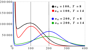
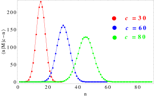
This modification forces the spatial volume at each slice to fluctuate around $n_{0}$. The new action leads to a modified transfer matrix but one can easily recover the original transfer matrix, as will be explained below. The modification of the action serves two purposes. Firstly, it allows us to determine the critical coupling $g_{c}$. The average volume distribution in the slices, for $T$ and $n_{0}$ sufficiently large, should have a maximum at $\langle n\rangle=n_{0}$. For finite $T$ we observe different distributions for different choices of $n_{0}$, but for $g=g_{c}$ the maximum should be stable. Typical distributions are shown in Fig. 1 for a system with four massive scalar fields with a mass $m^{2}=0.05$ and $g=g_{c}$.

Figure 1: Averaged volume distribution in a slice for a system with $d=4$ and $m^{2}=0.05$. We take $n_{0}=100,200$ and check the location of a maximum using $T=8$ and $T=14$.

This method can be used to determine the critical parameter $g_{c}$ even in cases, where the transfer matrix may not be a good approximation. In the table 1 we list the estimates for a range of mass parameters $m^{2}$ and, for comparison, for pure gravity. In the following we use $g=g_{c}$.

$m^{2}$	$g_{c}$ estimates	the best estimate $g_{c}$
0.00	0.2988-0.3000	0.2991
0.05	0.3205-0.3212	0.3210
0.10	0.33375-0.3338	0.33378
0.15	0.34412-0.34417	0.34415
0.20	0.35284-0.35285	0.35285
5.00	0.48322-.048342	0.48341
Pure gravity	0.4999-0.50	0.50

Table 1: Estimated values of $g_{c}$. The estimates come from volume distributions with $n_{0}=0,~{}50,~{}100,~{}150,~{}200$ and $T=20$.

Secondly, the modification (17) makes the spatial volume fluctuations much more controllable in the Monte Carlo simulations. It changes the probability distributions to

$$\tilde{P}_{T}(n_{1},n_{2},\dots,n_{T})=\frac{\langle n_{1}|\tilde{{\cal M}}|n_{2}\rangle\langle n_{2}|\tilde{{\cal M}}|n_{3}\rangle\cdots\langle n_{T}|\tilde{{\cal M}}|n_{1}\rangle}{\mathrm{tr}\,\tilde{{\cal M}}^{T}},$$ (18)

where the relation between ${\cal M}$ and $\tilde{{\cal M}}$ is given by

$$\langle n|{\cal M}|m\rangle=C^{\prime}e^{\frac{1}{2}\epsilon(n-n_{0})^{2}}\langle n|\tilde{{\cal M}}|m\rangle e^{\frac{1}{2}\epsilon(m-n_{0})^{2}},$$ (19)

again up to an arbitrary factor $C^{\prime}$. This relation permits us to determine the matrix elements $\langle n|{\cal M}|m\rangle$. The method will work for $n,~{}m$ restricted to a window around $n_{0}$, where volume fluctuations are small. The size of the window depends on the parameter $\epsilon$ and typically outside this window the fluctuations become large. In practice we measure the matrix elements for a sequence of $n_{0}$ and connect the results by requiring the best overlap.

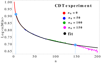
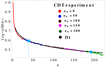
The transfer matrix, (10)-(11), depends on the two parameters $\mu$ and $\Gamma$. We determine $\mu$ by measuring the diagonal part of the transfer matrix (i.e. $\langle n|{\cal M}|n\rangle$), where the kinetic term vanishes. We use $T=8$. For $T>5$ the results seem insensitive to the periodic boundary conditions imposed in the time direction. As before we combine the measurements for various overlapping windows around different values of $n_{0}$. The results of best fits are shown in Fig.  2 for pure gravity (as a test of the method) and for $d=4$, $m^{2}=0.05$.

Figure 2: The logarithm of the diagonal of the transfer matrix at $g=g_{c}$ for pure gravity (left) and for $d=4$, $m^{2}=0.05$ (right). The plots show a combination of results obtained with $n_{0}=0,~{}50,~{}100,~{}150$. The black line represents a fit to the asymptotic power behavior of the diagonal part, with the coefficient determined in the range limit by the blue dots.

We determine $\Gamma$ by measuring the transfer matrix for $n+m$ fixed (such that only the kinetic term changes). For sufficiently large $c$ we have

$$\langle n|M|c-n\rangle=\mathcal{N}(c)\exp\left[{-\frac{(2n-c)^{2}}{\Gamma c}}\right],$$ (20)

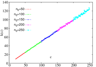
where the terms in the effective action which only depend on $c$ are included in the normalization. This is illustrated on Fig.  3, and we observe that the width of the Gaussian grows with $c$.

Figure 3: The transfer matrix $\langle n|M|c-n\rangle$ for various $c^{\prime}s$: pure gravity (left) and $d=4$, $m^{2}=0.05$ (right).

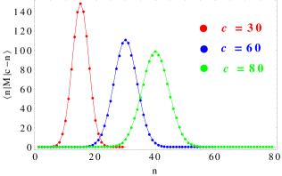
This growth is with a very high accuracy linear, as is illustrated on the figure 4.

Figure 4: Linear behavior of $k(c)\approx\Gamma c$ for pure gravity (left) and $d=4$, $m^{2}=0.05$ (right).

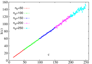
The fitted values of the parameters $\mu$ and $\Gamma$ are listed in the table 2.

$m^{2}$	0.05	0.10	0.15	0.20	5.0	Pure Gravity
$\mu$	0.64628	0.59365	0.55432	0.53233	0.503512	0.505763
$\Gamma$	2.5 $\pm 0.05$	2.2 $\pm 0.1$	2.17 $\pm 0.15$	2.15 $\pm 0.1$	2 $\pm 0.1$	2 $\pm 0.05$

Table 2: Estimated values of the parameters $\mu$ and $\Gamma$ as explained in the text.

As a check of the quality of the transfer matrix determined this way we performed a Monte Carlo simulation where the probability assigned to a geometry with spatial volumes $\{n_{1},n_{2},\dots,n_{T}\}$ is

$$P(n_{1},n_{2},\dots,n_{T})\propto\langle n_{1}|{\cal M}^{eff}|n_{2}\rangle\langle n_{2}|{\cal M}^{eff}|n_{3}\rangle\cdots\langle n_{T}|{\cal M}^{eff}|n_{1}\rangle e^{-\epsilon(\sum_{t}n_{t}-N)^{2}}.$$ (21)

The “effective” transfer matrix entries $\langle n_{1}|{\cal M}^{eff}|n_{2}\rangle$ used in (21) are

$$\langle n|{\cal M}^{eff}\ m\rangle=\begin{cases}\langle n|{\cal M}^{exp}|m\rangle,&m+n\leq K\\ \langle n|{\cal M}^{th}|m\rangle,&m+n>K.\end{cases}$$ (22)

The small volume part is obtained numerically and the large volume part is given by (10) and (11) with $\mu$ and $\Gamma$ determined as described above. $K$ is chosen in the range 50-100. The extra factor in (21) is added to enforce the total volume to fluctuate around a given value $N$. The resulting distribution can be compared to the one obtained using the full partition function (4). We use here the same method to analyze spatial volume profiles as that presented in [3, 4, 5]: each configuration is shifted in such a way that the “center of mass” of the spatial volume distribution is placed at time $t=T/2$. In this way we produce an artificial maximum also for pure gravity where there is no blob, but the properties of this distribution is quite different from the “real” blob distribution, as explained in [3, 4, 5] and as seen from Fig. 5.

Figure 5: Comparison of $n(t)/N$ using the effective transfer matrix and full CDT: pure gravity (left) and $d=4$, $m^{2}=0.05$ (right). We use $N=16000$, T=200 for both cases.

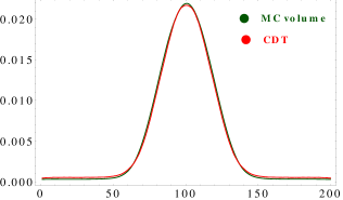
The agreement is very good. For the case $d=4$, $m^{2}=0.05$ the small volume part of the transfer matrix is important in order to get a quantitative agreement of the volume profile in the tail of the distribution (the agreement becomes less good at a quantitative level if $K<50$ in (22)) The existence or non-existence of the blob is however entirely linked to the value of $\mu$ in the effective action (11): simply using this effective action (with $g=g_{c}$) and adding a small volume term $1/(n+m)$ like in (9) in order to stabilize the logarithmic term for $n+m=0$ one obtains by Monte Carlo simulations a transition from a non-blob phase to a blob phase simply by changing $\mu$. $\mu$ is like a critical exponent: it is well know that $\mu=1/2$ appears as an entropy in CDT [2], and this is seen explicitly from (8) for large $n$:

$$\langle n|{\cal M}|n\rangle\sim(2n)^{-1/2}(g/g_{c})^{2n}(1+O(1/n)).$$ (23)

Changing the details of the triangulations used in CDT, changing the scale of $n$ etc, will change $g_{c}$ but not the exponent $\mu$. Similarly, when we couple CDT to the matter fields we have

$$\langle n|{\cal M}|n\rangle\sim(2n)^{-\mu}(g/g_{c})^{2n}(1+O(1/n)).$$ (24)

where $\mu$ will invariant under changes of triangulation details, but will depend on $d$ and $m$. Our numerical results suggest that there is a critical value $\mu_{c}$ such that for $\mu>\mu_{c}$ the geometry change universality class from that of pure CDT (with Hausdorff dimension $d_{H}=2$) to that the “blob” geometry (which has $d_{H}=3$).

3 Eigenvalue spectrum of the transfer matrix

The analytic solution of 1+1 dimensional CDT [2] permits us to determine the eigenvalue spectrum of the exact transfer matrix as a function of $g$. Using the parametrization

$$g=\frac{1}{2\cosh(\beta)},\quad g_{c}=\frac{1}{2}$$ (25)

and solving the eigenvalue equation we find (see also [9] for the eigenvalue spectrum for a more general model)

$$\lambda_{n}=e^{-(2n+2)\beta},\quad n=1,2,\dots$$ (26)

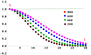
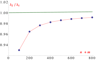
The effective transfer matrix determined above for $d=4$ was only obtained up to a normalization so we can only determine the ratio of eigenvalues for this “empirical” transfer matrix. For the pure CDT model we have $\lambda_{n}/\lambda_{1}=\exp(-2n\beta)$. Thus the ratio goes to zero exponentially with $n$ for $g<g_{c}$. For $g=g_{c}$ the spectrum becomes degenerate. In a numerical analysis we will never be able to achieve this limit, since our numerical transfer matrix is necessarily finite and the dependence on $n_{max}$ for $g=g_{c}$ for pure gravity is illustrated on the figure 6. We can see that at the critical point the convergence of the ratios to one is slow as function of $n_{max}$.

Figure 6: Left: Eigenvalues for pure gravity at $g=g_{c}$ with cut-off $n_{max}=200,400,600,800$. Right: $\lambda_{2}/\lambda_{1}$ as a function of $n_{max}$ .

We repeat the same analysis for the case $d=4$, $m^{2}=0.05$. The dependence of the eigenvalue spectrum at the critical point for various cut-off values $n_{max}$ is shown in Fig. 7. We see that even at the critical point the first few eigenvalues become cut-off independent. This can be attributed to a faster fall-off of the transfer matrix elements for large volumes.

Figure 7: Eigenvalues for $d=4$ $m^{2}=0.05$ and cut-off $n_{max}=200,~{}300,~{}400,~{}600$. The first four eigenvalues are essentially independent of $n_{max}$.

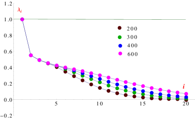
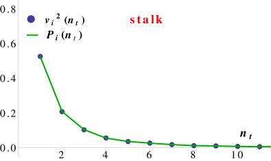
The eigenvalue spectrum is markedly different from the pure CDT case since the there is a gap between the first and the second eigenvalue even at $g=g_{c}$, a gap with does not vanish for large $n_{max}$. On the other hand the rest of the eigenvalues behave like the pure CDT eigenvalues in the sense that they coincide for growing $n_{max}$. The separation of the largest eigenvalue from the rest is a reflection of the existence of a stalk. In fact let us denote the first eigenvector (with the largest eigenvalue) $\nu_{1}(n)$. Fig. 8 shows that for small $n$ we have $\nu_{1}(n)^{2}=P(n)$, where $P(n)$ is the probability distribution for spatial volumes in the stalk (which is almost independent of $T$ and $N$).

Figure 8: The distribution of spatial volume in the “stalk” for $d=4$ and $m^{2}=0.05$ and the square of the first eigenvector of the transfer matrix.

4 Conclusions

In CDT there exists a transfer matrix. This transfer matrix depends on the geometry of the spatial slices. In 1+1 dimensions the geometry of the spatial slice is fully characterized by its length (assuming the topology is that of $S^{1}$). Once we couple the geometry to matter the transfer matrix still exists, but it will also depend on the matter degrees of freedom. Integrating out the matter degrees of freedom might introduce non-local interactions and invalidate any simple transfer matrix description in terms of geometry only. However, it turned out that for massive free Gaussian fields coupled to geometries, and for the mass not too small there is such an effective transfer matrix which describes very well the fluctuating geometry of the full model.

We determined the effective transfer matrix in 1+1 dimensional CDT coupled to 4 massive scalar fields with $m^{2}\geq 0.05$. 0.05 was the smallest value of $m^{2}$ where we could reliable determine an effective transfer matrix. We found that the most important term in the effective transfer matrix was an “entropic” factor $1/(n+m)^{\mu}$. $\mu$ is like a critical exponent, much like the entropy or susceptibility exponent $\gamma$ in non-critical string theory or the theory of dynamical triangulations. In the case of non-critical string theory $\gamma$ depends on the matter coupled to the 2D geometry and there is a phase transition between two completely different classes of geometries at $\gamma=0$. For $\gamma>0$ the two-dimensional geometry degenerates into so-called branched polymers. We have a somewhat similar scenario here: $\mu$ depends on $d$ and $m^{2}$ and there exists a $\mu_{c}$ such that for $\mu>\mu_{c}$ the geometry undergoes a phase transition and develops a “blob” with Hausdorff dimension $d_{H}=3$. The appearance of the blob had a profound impact on the effective transfer matrix. A gap developed between the two largest eigenvalues of the effective transfer matrix and the eigenvector corresponding to the largest eigenvalue was essentially equal to the square root of the probability distribution of spatial volumes of the stalk associated with the blob. We conjecture that a similar effective description of the blob–non-blob dynamics will be present for higher dimensional CDT where it has been shown that there also is an effective transfer matrix which describes distribution and fluctuation of the spatial volume of the time slices [10].

Acknowledgments. HZ is partly supported by the International PhD Projects Programme of the Foundation for Polish Science within the European Regional Development Fund of the European Union, agreement no. MPD/2009/6. JJ ac- knowledges the support of grant DEC-2012/06/A/ST2/00389 from the National Science Centre Poland. JA and AG acknowledge support from the ERC-Advance grant 291092, “Exploring the Quantum Universe” (EQU)