Spectral Clustering by Ellipsoid and Its Connection to Separable Nonnegative Matrix Factorization
Abstract
This paper proposes a variant of the normalized cut algorithm for spectral clustering. Although the normalized cut algorithm applies the K-means algorithm to the eigenvectors of a normalized graph Laplacian for finding clusters, our algorithm instead uses a minimum volume enclosing ellipsoid for them. We show that the algorithm shares similarity with the ellipsoidal rounding algorithm for separable nonnegative matrix factorization. Our theoretical insight implies that the algorithm can serve as a bridge between spectral clustering and separable NMF. The K-means algorithm has the issues in that the choice of initial points affects the construction of clusters and certain choices result in poor clustering performance. The normalized cut algorithm inherits these issues since K-means is incorporated in it, whereas the algorithm proposed here does not. An empirical study is presented to examine the performance of the algorithm.
1 Introduction
Clustering is a task of dividing a data set into groups on the basis of similarities between pairs of data points. The task is to find groups of data points such that similar data points are in the same group and dissimilar ones in different groups. Here, the groups found by an algorithm for the clustering task are referred to as clusters. Spectral clustering is a graph-based clustering, and the eigenvalues and eigenvectors of the graph Laplacian play a central role.
In spectral clustering, we construct a weighted graph to represent the similarities of data points. The vertices correspond to data points, and the edges are associated with weights. The weights are determined by a similarity function that quantifies the similarity of two data points; it takes on a large positive value if the data points are similar, while it gets close to a zero value if they are dissimilar. Small weights are usually ignored when constructing the graph since they may not make a major contribution to the configuration of clusters. For each data point, we pick up some data points with high similarity with it, and put edges with positive weights between them. An input parameter , called the neighbor number, determines how many data points are chosen.
In the weighted graph, the clustering task is to divide the vertex set into groups such that the total edge weight in the same groups is large, while those among different groups are small. Shi and Malik in [22] introduced a normalized cut function to formulate this task. The function assigns a nonnegative real number to the groups of vertices, and it reaches its minimum when the task is completed. The ideal goal is to find groups of vertices that minimize a normalized cut function.
However, finding the optimal solution of the normalized cut minimization problem is hard. We instead solve a relaxation problem formed by dropping hard constraints. This is an eigenvalue problem for a normalized graph Laplacian. The eigenvalues and eigenvectors of the Laplacian contain clues for finding the optimal solution of the normalized cut minimization problem. Thus, we attempt to find clusters by using them. The normalized cut algorithm proposed by Shi and Malik in [22] and Ng et al. in [21] applies a K-means algorithm to the eigenvectors. We will use the abbreviation NC to denote this algorithm for short.
Instead of K-means in NC, we propose to use the minimum volume enclosing ellipsoid for the eigenvectors of normalized graph Laplacian. The computation of such an ellipsoid can be formulated as a convex optimization problem, and there are efficient algorithms for solving it. Our algorithm computes the enclosing ellipsoid and chooses some points lying on the boundary by using the successive projection algorithm (SPA) of [11]. The points can be thought of as representatives of the clusters. Hence, our algorithm assigns data points to the representative points on the base of their contribution. The assignment can be formulated as a convex optimization problem. Figure 2 of Section 7.2 illustrates the algorithm.
We see in Theorem 1 that the algorithm has a similarity to the ellipsoidal rounding (ER) algorithm for separable nonnegative matrix factorization (NMF) in [20] when the neighbor number is set to be equal to the number of data points, in other words, when all weights are taken into account in constructing the graph. Strictly speaking, the final outputs returned by these two algorithms do not coincide. However, we see in Corollary 1 that the outputs coincide if we modify one step of ER. Accordingly, our algorithm can be thought of as an extension of ER. A separable NMF is a special case of NMF, and it has applications in clustering and topic extraction of documents [5, 3, 20] and in endmember detection of hyperspectral images [10, 11]. It is a matrix factorization problem, and basically differs in purpose from spectral clustering. However, the theoretical insights shown here imply that our algorithm can serve as a bridge between spectral clustering and separable NMF through neighbor number .
The K-means algorithm has the issues in that the choice of initial points is sensitive to the way clusters are constructed; some choices yield good clustering performance, while others do not. It is difficult to choose good initial points before running the algorithm and the choice affects the cluster construction. Hence, NC inherits the issues. There have been many studies indicating that NMF based clustering within the block coordinate descent (BCD) framework has a good performance. However, the framework has similar issues as K-means. Our algorithm does not have these issues, since it consists of solving an eigenvalue problem and convex optimization problems and performing SPA.
We conducted experiments evaluating the performance of our algorithm on real image data sets and compared its results with those of existing algorithms, including NC and NMF. We set multiple initial points for the existing algorithms and measured the worst, best, and average performance. The experimental results showed that the performance of our algorithm is higher than the average performance of the existing algorithms in almost all cases. We observed that there are initial points that result in the existing algorithms having poor performance, and as a result, their average performance gets worse. We also conducted experiments to see how the performance our algorithm varies with the neighbor number .
The rest of this paper is organized as follows. After introducing the notation and symbols, we review the NC algorithm in Section 2. Our algorithm is presented in Section 3, and its connection with the ER algorithm is shown in Section 4. We mention the issues of initial point choice in NC and ER in Section 5, and review related work in order to discuss the relationship between spectral clustering and NMF in Section 6. An empirical study is reported in Section 7. Finally, concluding remarks are given in Section 8.
1.1 Notation and Symbols
We use and to denote the set of -by- real matrices and -by- nonnegative matrices. Here, a nonnegative matrix is a real matrix whose elements are all nonnegative. We also use to denote the set of -by- real symmetric matrices. Let be a matrix of proper size. The symbol represents its transpose. The symbols and represent the trace and rank. We use and to denote a vector of all ones and an th unit vector. We use to denote an identity matrix. The symbol represents an -by- diagonal matrix such that diagonal elements are . Let and be a -by- matrix and a -by- matrix. We use to denote the horizontal concatenation of the two matrices and the matrix size is -by-. For a set , the symbol represents the number of elements, and the symbol is the complementary set.
2 Review of Normalized Cut Algorithm for Spectral Clustering
We denote data points by -dimensional vectors , and its set by . Consider subsets of . If the subsets are disjoint and its union coincides with , we call the subsets disjoint partitions of . In this paper, we consider clustering algorithms to return the disjoint partitions of , and call the disjoint partitions returned by them clusters of data points. Spectral clustering is a graph-based clustering, and the algorithm is based on the eigenvalue decomposition of a graph Laplacian. There are some types of algorithms proposed for spectral clustering. In particular, the NC algorithm by Shi and Malik of [22] and Ng et al. of [21] is popular and often used. For the details of algorithms and history in spectral clustering, we refer the reader to the survey paper [26]. Below, we review the NC algorithm.
In spectral clustering, we set a function on a weighted graph , and formulate a clustering task as a problem of minimizing . A weighted graph is a graph such that each edge is associated with a weight. Let and denote the sets of the vertices and edges. The weight value is given by a function from to a set of nonnegative real numbers. An edge links two vertices and if the value of at is positive; otherwise, it does not link. For an edge between two vertices and , let denote the value of at . Consider a subset of vertex set . We use the notation to denote the total weight of all edges between and its complement . Namely,
In the same manner to [26], hereinafter, we use a shorthand notation . This notation represents the indices of vertices in . A degree of vertex is the total weight of all edges connected to , and we denote it by . We use the notation to denote the total degree of all vertices in . Namely,
where is a degree of vertex in and it is given as for the weights on edges . The can be regarded as the size of .
The NC algorithm consists of three major steps. The first step constructs a weighted graph . A vertex is in one-to-one correspondence with a data point . Let be a function that quantifies the similarity of two data points. The function assigns a nonnegative real number as the similarity of data points and ; it takes on a large positive value if the data points are similar, while it gets close to a zero value if they are dissimilar. In the context of spectral clustering, the function is referred to as a similarity function. A polynomial function and a Gaussian function are popular and often used as the function. In particular, this paper deals with the former function, and its form is
| (1) |
where is a nonnegative real number and is a positive integer number. These are parameters given in advance.
Small weight values in may not make a major contribution to the configuration of clusters, and thus, are usually ignored. A -nearest neighbor set is used for this purpose. For a data point , we choose the top data points with high similarity to as measured by a similarity function , and construct a set by collecting these points. Let denote the set. The integer number used for the construction is referred to as a neighbor number. The weight value of is given as
We denote the -by- symmetric matrix consisting of by . The matrix is called a weighted adjacency matrix of , and in this paper, it is referred to as an adjacency matrix for short.
The next step finds clusters from the graph built in the first step. A graph Laplacian is a matrix so as to possess some properties of . To see the form of this matrix, we need to introduce a degree matrix. A degree matrix of is a diagonal matrix whose diagonal element is the degree of each vertex. Namely, the th element is given as where is an element of the adjacency matrix of . We denote the -by- diagonal matrix by . A degree matrix is usually assumed to be nonsingular. The singularity means that some data point is isolated and is completely dissimilar to all the other data points. Thus, such a data point should be removed. A graph Laplacian of is a matrix given as for a degree matrix and an adjacency matrix . This is an -by- symmetric matrix, and we denote it by .
We set a function to find the clusters from . Although some choices are possible, we consider the function for the disjoint partitions of ,
| (2) |
This function is called a normalized cut. Other types of functions have been proposed in this context. For instance, a ratio cut function [12] is as popular as the normalized cut one. The takes a small value if the data points in and are dissimilar. The takes a large value if so is the size of . Therefore, the minimization of the normalized cut function is to find the clusters such that the data points in different clusters are dissimilar and the cluster sizes are large.
The ideal goal is to find disjoint partitions of minimizing the normalized cut function. To be precise,
(Spectral clustering by the normalized cut function) Suppose that we are given a data set and an integer number . Find the disjoint partitions of to minimize the normalized cut function of (2).
The optimal solution of the minimization problem provides the best clusters in the sense that it attains the minimum of . But, this is a hard combinatorial problem, and thus we consider its relaxation problem. By using a graph Laplacian , we rewrite as
Here, is an -by- matrix determined by , and its element is
| (3) |
Therefore, the minimization problem of is equivalent to the problem,
The hardness of this problem is in the constraint for . Hence, we drop the hard constraint. Instead, we take into account that satisfies the relation and add it as the constraint. Namely, we consider the problem,
The problem serves as the relaxation problem of . It can be solved through eigenvalue decomposition. By introducing a new matrix variable such that , we transform the problem into an equivalent one,
In this transformation, we use the assumption that a degree matrix is nonsingular, and in other words, the diagonal elements are all positive. The optimal value and solution of is obtained from the eigenvalue decomposition of normalized graph Laplacian . We arrange the eigenvalues in ascending order, and let denote the values. Namely, the relation holds. Also, let denotes the eigenvector corresponding to the eigenvalue for . We easily see that the optimal value and optimal solution of are given as and such that and . Therefore, those of are respectively and .
The final step constructs clusters from the optimal solution of relaxation problem . We search for the optimal solution of original problem based on clues provided by that of . Let us see the matrix of in detail. We take the transpose of , and denote the column vectors of by . The vector can be regarded as an indicator to tell us which cluster a data point belongs to. The elements of are all zero except one element, and the position of nonzero element indicates the cluster index to which a data point belongs. The convex hull of is an -dimensional simplex in . Among , there are different types of vectors and those different ones correspond to the vertices.
Let us consider the situation in which the optimal solution of relaxation problem is close to the optimal solution of original one . In the same way as , we take the transpose of and denote the column vectors of by . Under this situation, we can have an expectation that the convex hull of is similar to the shape of an -dimensional simplex, and are located around each vertex of the simplex. Thus, these vectors should form clusters. Accordingly, the clusters can be found by applying a clustering algorithm such as K-means to . Algorithm 1 describes each step of the algorithm by Shi and Malik in [22].
Input:
A data set , a cluster number , a neighbor number ,
and a similarity function .
Output: Clusters .
-
1:
Construct an adjacency matrix by using a similarity function and a -nearest neighbor set.
-
2:
Let and be a graph Laplacian and a degree matrix obtained from . Compute the eigenvectors of the normalized graph Laplacian in correspondence with the smallest eigenvalues.
-
3:
Form a matrix , and let be the columns of .
-
4:
Apply the K-means algorithm to , and find clusters .
3 Proposed Algorithm
In this section, we will describe the proposed algorithm. The algorithm is a variant of the NC algorithm. Although NC uses K-means for the construction of clusters in the final step, it instead uses a minimum volume enclosing ellipsoid (MVEE).
3.1 Observation for the Optimal Solution of
Our algorithm is built on the following observation.
Observation 1.
Let denote the column vectors of . The convex hull of has a similar shape to an -dimensional simplex in , and are around the vertices. Therefore, these vectors form clusters in the neighborhood of the vertices.
As mentioned in the last of Section 2, this observation should hold if is close to the optimal solution of . We see in Proposition 1 that the lie on a hyperplane, and thus, its convex hull is at least an -dimensional polytope. In the following description, we use the same notation in Section 2; are the eigenvectors of normalized graph Laplacian , and those correspond to each of the eigenvalues with ; are the column vectors of with given by the .
Proposition 1.
can be chosen as with some nonzero real number . Thus, if we choose as , then, lie on a hyperplane .
Proof.
It suffices to show the first part of this statement that can be chosen as . Let denote a normalized graph Laplacian . Since a graph Laplacian is positive semidefinite, so is . Also, we have . Thus, has a zero eigenvalue as the smallest one, and the corresponding eigenspace contains a vector with some nonzero real number . ∎
Regarding the first part of the proposition, we can find the same statement in Proposition 3 of [26].
Remark 2.
Although Proposition 1 requires us to choose the vector from the eigenspace associated with the smallest eigenvalue, eigenvalue solvers such as eig and eigs commands on MATLAB do not always output the vector. But, we, of course, can reconstruct it from the eigenvectors provided by the solvers. Let denote the eigenspace in associated with the smallest eigenvalue. Suppose that the dimension of is . Since a normalized graph Laplacian is a symmetric matrix, we can take orthonormal basis vectors for . Let denote the orthonormal basis vectors. Then, there exists a nonzero vector such that and where since . We pick up orthonormal basis vectors for the orthogonal complement to . Let . We construct . Since is an orthogonal matrix, the column vectors of are the orthonormal basis vectors spanning , and the first column vector is .
3.2 MVEE for the Points in Simplex
Observation 1 implies that form clusters in the neighborhood of the vertices of an -dimensional simplex in . Thus, if we can find vectors from that are close to the vertices of the simplex, those vectors should serve as the representative points of clusters. An MVEE for can be used for finding such vectors. This is because it can touch the near-vertices if the convex hull of is similar to the shape of simplex. Originally, this geometric property has been shown in [10, 20] in order to design algorithms for a separable NMF problem.
In this section, we first see the formulation of MVEE, and then recall the precise description of the property in Propositions 2 and 3. Let be an -by- positive definite matrix, and be an -dimensional vector. A full-dimensional ellipsoid in is defined as a set . The vector serves as the center of ellipsoid . In particular, an ellipsoid is referred to as an origin-centered ellipsoid if the center matches the origin (in other words, is a zero vector). It is known that the volume of unit ball in only depends on the dimension , and we denote it by . The volume of is given as . Let denote the boundary of such that . A vector is called as an active point of if it lies on the boundary such that .
Let be points in . We put the following assumption on the points.
Assumption 1.
for .
We consider an origin-centered ellipsoid to enclose the convex hull of a set , and describe several properties of the enclosing ellipsoid with minimum volume. Assumption 1 ensures that the convex hull of is full-dimensional in , and thus, the enclosing ellipsoid has a positive volume. The volume minimization of enclosing ellipsoid for the convex hull of is formulated as the problem,
The -by- matrix is the decision matrix variable. The symbol for a matrix represents that it is positive definite. In the problem , we need to put Assumption 1 to ensure the existence of optimal solution. Let denote the optimal solution. The set is an origin-centered enclosing ellipsoid with minimum volume for the convex hull of . This paper refers to it as an origin-centered MVEE for . The active points of the origin-centered MVEE are the points satisfying . The problem is a convex optimization problem, and there are polynomial-time algorithms for solving it. The problem and algorithms for computing an MVEE have been well studied, and we refer the reader to, for instance, [6] for the details.
We describe the propositions mentioned in the first of this section.
Proposition 2 (Lemma 11 of [20]).
Suppose that satisfy Assumption 1. Then, the origin-centered MVEE for touches at least points with plus-minus signs among .
Proposition 3 (Proposition 3 and Corollary 4 of [20]).
Consider an -dimensional simplex in . Let be the vertices, and let .
-
(a)
Suppose that belong to the simplex. Construct a set . Then, the origin-centered MVEE for only touches the vertices with plus-minus signs.
-
(b)
Suppose that are given as by using such that . Construct a set . Then, the origin-centered MVEE for only touches the vertices of with plus-minus signs.
The proof for Proposition 3(a) is also found in [10]. Proposition 3(b) can be thought of an extension of that of Proposition 3(a) in some sense since in Proposition 3(a) can be written as by using such that and . It should be noted that Assumption 1 is satisfied in Proposition 3 since are the vertices of -dimensional simplex.
We see from Proportions 2 and 3 that the following geometric properties hold. Consider a finite number of points, including the vertices, in an -dimensional simplex in . Then, the origin-centered MVEE for the points touches the vertices. Furthermore, it also holds even if some amount of perturbation is added to the points. If the perturbation is large, the ellipsoid can touch more that points.
3.3 Algorithm Description
Recall Observation 1; are the column vectors of whose transpose is the optimal solution of problem . Suppose that Observation 1 holds. Then, the convex hull of is similar to the shape of a simplex. Proposition 3 tells us that the MVEE for the set can touch some vectors among that are close to the vertices of the simplex. Such vectors should serve as the representative points of clusters. Accordingly, clusters can be found by assigning to the representative points on the base of their contribution. Here, we should pay attention to the following issue. Proposition 2 implies that the MVEE for the has a possibility to touch more than vectors among . The algorithm for a separable NMF problem such as SPA [11] can be used for selecting points from the candidates. We will explain the problem and algorithms in Section 4.1.
Input:
A data set , a cluster number ,
a neighbor number , and a similarity function .
Output: Clusters .
-
1:
Run steps 1-3 of Algorithm 1, and let where these vectors are the columns of .
-
2:
Compute an origin-centered MVEE for the set , and find all active points. Let be the index set of the active points.
-
3:
If , set as . Otherwise, select elements from by SPA, and construct the set of these elements.
-
4:
Assign each to any one of on the base of contribution, and construct clusters .
Our algorithm is presented in Algorithm 2. We denote it by NCER since it is a variant of NC and uses an ellipsoid rounding to find clusters in the final step. Below, we explain the details of steps 3 and 4.
We see from Proposition 2 that the index set of active points constructed in the step 2 contains at least elements since the vectors satisfy for . Therefore, step 3 constructs a set by setting if ; otherwise, selects elements from , and constructs a set . SPA can be used for the selection. If the convex hull of vectors is similar to the shape of a simplex, SPA can select vectors from that are close to the vertices of the simplex. We refer the reader to Algorithm 1 of [11] for the details of SPA.
Step 4 assigns to representative points , and constructs clusters. The assignment is conducted on the base of contribution rate of representative points in generating a point. Let denote an matrix consisting of the representative points . Namely, . Consider some . We define a contribution rate of the representative points to as the optimal solution of the problem,
The -dimensional vector is the decision variable. This is a convex optimization problem, and sometimes referred to as a nonnegative least square (NLS) problem. The optimal solution can be obtained by using an active set algorithm. We refer the reader to [16] for the details of the algorithm. Let be the optimal solution of the problem. We find the index of the largest element among the elements of , and assign to a cluster .
4 Connection to Separable NMF
In this section, we will see that NCER for spectral clustering is closely related to ER for separable NMF in [20]. In fact, NCER shares similarity with ER when a neighbor number is set to be equal to the number of data points.
4.1 Separable NMF Problem
Consider a -by- nonnegative matrix such that
| (4) |
Here, is an -by- identity matrix, is an -by- nonnegative matrix, and is an -by- permutation matrix. A nonnegative matrix is called a separable matrix if it can be decomposed into and of the form (4). We call the a basis matrix and the a weight matrix. A separable NMF problem is a problem of finding the basis and weight matrices from a separable matrix. To be precise,
(Separable NMF problem) Suppose that we are given a separable matrix of the form (4) and an integer number . Find an index set with elements such that .
Here, denotes the submatrix of which consists of the column vectors with indices in . Namely, for the column vectors of .
A separable NMF is the special case of NMF. As we will mention in Section 5, solving an NMF problem is hard in general. As a remedy for the hardness, Arora et al. in [4, 5] proposed to make the assumption called separability on the NMF problem. Then, it turns into a tractable problem under the assumption. An NMF problem under a separability assumption is referred to as a separable NMF problem. Separable NMF has applications in clustering and topic extraction of documents [4, 5, 15] and endmember detection of hyperspectral images [10, 11].
We shall look at the separable NMF problem from geometric point of view. Since the data matrix is a separable one of the form (4), the conical hull of the column vectors of is an -dimensional cone in . It has extreme rays, and those correspond to the column vectors of basis matrix . The intersection of the cone with a hyperplane is an -dimensional simplex in , and the vertices correspond to the column vectors of basis matrix . Figure 1 illustrates the geometric interpretation of separable matrix. Hence, a separable NMF problem can be rewritten as a problem of finding all vertices of -dimensional simplex in . Several types of algorithms have been proposed for a separable NMF problem. SPA[11] and XRAY[15] as well as ER are designed on the geometric interpretation of separable matrix.
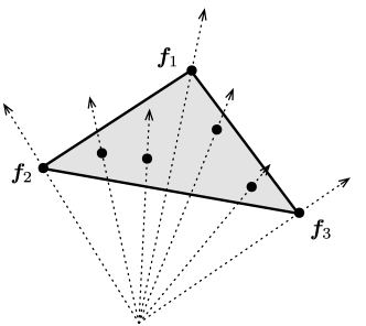
It is ideal that an algorithm for a separable NMF problem is robust to perturbation which disturbs the separability structure. For a separable matrix of (4) and a -by- real matrix , we consider the matrix
| (5) |
We call the a near-separable matrix since the separability structure of is disturbed by . A separable NMF algorithm is said to be robustness if the algorithm can find a matrix close to the basis matrix in a near-separable matrix. It has been shown theoretically and practically in [20] and [11] that ER and SPA are robust algorithms.
4.2 ER Algorithm
We give a precise description of ER. As already mentioned, the algorithm is based on the geometric interpretation of separable matrix, and Propositions 2 and 3 are the backbone of the algorithm. In the application of Proposition 3 to a separable NMF problem, we need to pay attention to the following point. The proposition requires that an -dimensional simplex is in an -dimensional real space. But, in the problem, it can be in higher dimensional space. Therefore, a dimension reduction is required to be performed.
Input: A -by- nonnegative matrix , and a basis number .
Output: An index set .
-
1:
Perform a dimension reduction of from to and construct a dimensionally reduced matrix through SVD.
-
2:
Remove all of zero column vectors in if exist. Construct a diagonal matrix such that all column vectors of lie on a hyperplane . Let for the column vectors of .
-
3:
Compute an origin-centered MVEE for the set , and find all active points. Let be the index set of the active points.
-
4:
If , set as . Otherwise, select elements from by SPA, and construct the set of these elements.
Algorithm 3 describes each step of ER. In the description, the notation is still used to denote the number of column vectors of for simplicity although it varies if the zero column vectors of are removed in the step 2. We explain the details of the steps 1 and 2 although the steps 3 and 4 are the same as the steps 2 and 3 of NCER.
Step 1 computes the singular value decomposition (SVD) of . The SVD of takes the form
| (6) |
is a -by- orthogonal matrix consisting of left singular vectors . is an -by- orthogonal matrix consisting of right singular vectors . is a -by- diagonal matrix consisting of singular values with the relation . Here, the is a -by- zero matrix. We pick up the largest singular values , and construct the -by- diagonal matrix . The matrix is known to be the best rank- approximation matrix to in measured by matrix -norm. Here, for the column vectors of , and for those of . It should be noted that we have if is a separable matrix. After the SVD computation of , step 1 constructs
We call the matrix a dimensionally reduced matrix for .
Step 2 constructs a diagonal matrix that scales the column vectors of to lie on a hyperplane. There exists such a hyperplane since has no zero column vectors. We consider a hyperplane . Here, is a -dimensional real vector such that the elements are all nonzero and is a nonzero real number. The intersection points of column vectors of with are given as for . Thus, in this step, we construct by using the .
We need to put an assumption on a basis number which is set as an input parameter in advance. Step 3 computes an MVEE for the column vectors of . In the MVEE computation, Assumption 1 needs to be satisfied and the computation is allowed under the assumption. Therefore, we put an assumption on a basis number that for a data matrix . If the assumption holds, the largest singular values of are positive, and thus, we have .
ER has been shown in [20] to have the following properties. Let be a separable matrix of the form (4). Then, ER for an input data with returns the index set such that . Let be a near-separable matrix of the form (5). If satisfies , then, ER for an input data with returns the index set such that . Here, is a nonnegative real number determined by the basis matrix and weight matrix . For the details, we refer the reader to Theorem 9 of the paper.
Remark 4.
The original description of ER in [20] does not contain the step 3 of the above algorithm description. If the input data matrix is a separable one, we can assume without loss of generality that the column vectors of lie on a hyperplane. This is because we have for nonsingular matrices and . Hence, we can skip the step 3 if is a separable matrix and the column vectors of are scaled to lie on a hyperplane in advance.
4.3 Connection between NCER and ER Algorithms
We observe the active point sets constructed in the step 2 of NCER and the step 3 of ER, and then, see that the two sets coincide with each other under some assumptions on data points and parameters of the algorithms. In the next steps, the algorithms select elements from the active point sets, and construct sets by collecting them. The two sets are different in general. But, we see that those sets coincide if we modify one step of ER.
We put an assumption on data points for NCER and ER.
Assumption 2.
Any of data points are nonnegative and not a zero vector.
The first part of Assumption 2 is required for ER. In below discussion, we need to handle a diagonal matrix
| (7) |
for data points . The second part of Assumption 2 is used to ensure that the is nonsingular. Let for the data points . We put assumptions for the parameters of NCER and ER.
Assumption 3.
For the NCER algorithm, we have the following settings.
-
(a)
A similarity function in the input is set as .
-
(b)
A neighbor number in the input is set as .
Assumption 4.
Let be of (7). For the ER algorithm, we have the following settings.
-
(a)
A data matrix in the input is set as .
-
(b)
A basis number in the input is set as satisfying .
-
(c)
A diagonal matrix in the step 2 is set as .
It should be noted that the in Assumption 4 is nonsingular under Assumption 2. Assumption 3(a) chooses a polynomial function of (1) with and as a similarity function. This function gives a similarity of two data points as its inner product. Assumption 3(b) means not to ignore small values of similarity, and take into account all the values in a graph. Assumption 4(a) scales the data points into by the diagonal elements of . We give a remark on this assumption in the last of this section. We see below that the corresponds to a degree matrix of a graph constructed by the similarity function and -nearest neighbor set under Assumption 3. As mentioned in the last part of Section 4.2, Assumption 4(b) ensures to allow us to carry out an MVEE computation in the step 3 of ER. We see below that Assumption 4(c) makes the column vectors of dimensionally reduced matrix lie on a hyperplane.
Theorem 1.
We prove this theorem in the remaining of this section. First, we shall see in detail how vectors in the step 1 of NCER are constructed under Assumptions 2 and 3. For the data points , we let . Under the assumptions, a graph Laplacian for the data points is
| (8) |
Here, is a degree matrix for an adjacency matrix , and its form is given as (7). The normalized graph Laplacian is of the form . Hence, the eigenvalue decomposition of can be obtained through the SVD of . In a similar way to the description of (6), we write it as
| (9) |
Here, and are respectively -by- and -by- orthogonal matrices, and the column vectors are respectively the left and right singular vectors of . is a -by- diagonal matrix , and are the singular values of . The eigenvalue decomposition of can be written as
| (10) | |||||
by using the expressions (8) and (9). We arrange the eigenvalues of in ascending order, and denote the th eigenvalue by . Namely, holds. Then, from the expression (10), we have
for . Here, the relation comes from the fact that a normalized graph Laplacian is positive semidefinite and has a zero eigenvalue. The column vector of is the eigenvector of , and corresponds to the eigenvalue and also singular value . Let . Under the assumptions, we see that in the step 1 of NCER are the column vectors of
| (11) |
and the column vectors of are the right singular vectors of in correspondence with the largest singular values with .
Next, we shall see in detail how vectors in the step 2 of ER are constructed under Assumptions 2 and 4. Under the assumptions, step 1 computes the SVD of and constructs a dimensionally reduced matrix for the matrix. Since the is equivalent to the degree matrix constructed in NCER under Assumptions 2 and 3, the SVD of coincides with that of (9). Let for the right singular vectors in correspondence with the largest singular values such that . The last strictly inequality comes from Assumption 4(b). Also, let for the singular values . Then, the dimensionally reduced matrix is given as by using those and . From Assumption 4(b), Step 2 constructs
| (12) |
by using of (7). The and coincide with those of (11). As already shown in (10), the corresponds the eigenvectors of normalized graph Laplacian for of (8). We see from Proposition 1 that of (12) does not have any zero column vectors and the column vectors lie on a hyperplane for some nonzero real number .
The column vectors of in (12) can be thought of as the images of those of in (11) under a linear transformation . This transformation is nonsingular since are all positive under Assumption 4(b). It is well known that an MVEE computation is invariant under a nonsingular linear transformation; see [6] for instance. Therefore, the following proposition holds.
Lemma 1.
Let be a nonsingular matrix. Consider such that for . Let be the set of active points in the origin-centered MVEE for a set and be that for a set . Then, we have .
Proof.
The origin-centered MVEEs for each of sets and are given by the optimal solutions of problems and . We denote by and the optimal solutions of and . Then, we have . Therefore, the active point set of origin-centered MVEE for coincides with that for . ∎
The proof of Theorem 1 is now obtained.
The step 3 of NCER and also the step 4 of ER select elements from the active point sets, and construct the index sets of the elements. Although the two index sets are different in general, those coincide if we modify one step of ER. In the step 1, we set as instead of . We denote the modified version of ER by MER. We immediately have the following corollary.
Corollary 1.
Accordingly, if we perform MER, and classify after the step 4 by following the step 4 of NCER, then, the obtained clusters coincide with those by NCER under the three assumptions. We will give the demonstration in Section 7.4.
5 Issues in Clustering by K-means and NMF
We recall the algorithms in K-means and NMF clustering, and then, mention the issues about the choice of initial points. An empirical study will be reported to confirm the issues in Subsection 7.3. Given a data set and an integer number . Let denote a data point in . In K-means, we set the function for the disjoint partitions of ,
where
| (13) |
and consider the problem of minimizing the function . The serves as a center of the partition . Although, conventionally, the number of partitions is denoted by in K-means, we continue to use for consistency in this paper. The minimization problem is hard to solve, and in fact, has been shown to be NP-hard in [9, 2]. Thus, instead of the global optimal solution, we find the local solution by using an alternative procedure. We minimize by alternatively fixing centers and partitions . When are fixed, a data point is assigned to having the nearest center such that the index attains the minimum value of for . When are fixed, is computed by following (13). The K-means algorithm repeats the procedure until some stopping criteria are satisfied. To start the alternative procedure, it requires us to arbitrarily choose and fix them in advance. It is empirically known that the choice of initial centers is sensitive to the cluster construction; some choices may make it possible to show good clustering performance, while others may not. It is difficult to choose good initial points before running the algorithm and the choice affects the cluster construction. NC has the same issues since K-means is incorporated in it.
Given a -by- nonnegative matrix and an integer number . The column vectors of correspond to data points. In NMF, we find a -by- nonnegative matrix and an -by- nonnegative matrix such that the product of and is as close to as possible. A natural way for the formulation is that we set the function for matrices and
| (14) |
and consider the problem of minimizing the function under the nonnegativity constraints on and . Solving the problem is hard, and has been shown to be NP-hard in [25]. However, the intractable problem can be reduced into tractable subproblems if either of or is fixed. Each subproblem becomes a easily solvable NLS problem. The NMF algorithm repeats to solve NLS problems by alternatively fixing and so as to minimize until some stopping criteria are satisfied. This alternative procedure can be regarded as a BCD framework which is used for minimizing a nonlinear function; see [14] for the details of the framework. After that, the algorithm classifies data points to clusters by using the obtained and . The assignment is similar to the step 4 of NCER. We regard the column vectors of as the representative points of clusters, and the elements of column vectors of as a contribution rate. For a column vector , we find the index of the largest element in , and assign a data point to the th cluster . The NMF algorithm employs a BCD framework, and it requires us to arbitrarily choose (or ) and fix it in advance. As is the case in K-means, the choice of initial matrix is sensitive to the cluster construction.
There are many studies on the efficient implementation of NMF algorithm. The main discussion points are in how to solve NLS problems. Although various types of algorithms are proposed, the multiplicative update algorithm of [17] may be the most popular one. Empirical results in [18] and [13] imply that a projected gradient algorithm and an active set algorithm are faster and provide more accurate solutions than a multiplicative update. We refer the reader to [14] for further discussion.
We finally mention the GNMF algorithm proposed in [7]. Empirical results in the paper imply that GNMF outperforms NC and NMF in clustering. This is a variant of the NMF algorithm. In GNMF, we add the regularization term to the function of (14), and set the function
| (15) |
where
The problem we consider is to minimize the function under the nonnegative constraints on and . Here, are the elements of adjacency matrix which is constructed for data points , and is the corresponding graph Laplacian. Also, is a parameter and takes a nonnegative value. The term is called a graph regularizer. We interpret as a dimensionally reduced data matrix for . If data points and are similar to each other, the term forces the dimensionally reduced ones and to be similar. The GNMF algorithm minimizes by using a BCD framework, and solves subproblems by using an algorithm based on the notion of the multiplicative update. After that, it applies K-means to the column vectors of , and finds clusters. Accordingly, there are two parts in GNMF that require us to set initial points in advance.
6 Related Work on Connection of Spectral Clustering and NMF
Some of previous studies discuss the relationship between spectral clustering and NMF. In particular, the paper [8] points out that a similarity can be found in the problem formulations in spectral clustering and NMF. We again consider the normalized cut minimization problem . Since the matrix variable are nonnegative, we construct the following relaxation problem by taking account of it.
Under the change of variable , this is equivalent to
since is a diagonal matrix such that the diagonal elements are all positive. Furthermore, the object function is and we have . We here let . Thus, the above relaxation problem is essentially equivalent to
Hence, if we drop the orthogonal constraint from there, then, it can be thought of as the special case of NMF since is a nonnegative matrix. However, to the best of the author’s knowledge, there may be no work to rigorously discuss the similarity of algorithms for spectral clustering and NMF.
7 Experiments
We will show an empirical study to investigate the performance of NCER. The first experiments visualize the products obtained from NCER for a small data set. In the experiments, we will see the relationship between the performance of NCER and Observation 1. The second experiments compare the performance of NCER with existing algorithms. The third experiments display how the performance of NCER varies with the neighbor number . All experiments were conducted on a 3.2 GHz CPU processor and 12 GB memory.
7.1 Algorithm Implementation, Data Sets, and Measurements
All algorithms used in the experiments were implemented on MATLAB. We describe the implementation details as follows.
-
•
NCER. Three computation require to be carried out: eigenvalue and eigenvector computation, MVEE computation, and NLS problem solving. We used MATLAB commands eigs and lsqnonneg for the first and third computation. The lsqnonneg employs the active set algorithm for an NLS problem. For the second computation, we performed the interior-point algorithm in a cutting plane framework. It has been shown empirically in [23, 1] that the use of cutting plane accelerates the efficiency of interior-point algorithm for an MVEE problem, and makes it possible to handle large problems. We used the software package SDPT3 [24] to perform the interior-point algorithm.
-
•
NC. In addition to eigenvalue and eigenvector computation, K-means requires to be performed. We used a MATLAB command kmeans for performing it and the eigs command.
-
•
NMF. NLS problems require to be solved in the BCD framework for minimizing of (14). As mentioned in Section 5, there are various possibilities for the choice of algorithms for solving NLS problems. We used the code available from the author’s website of [18]. The code employs the projected gradient algorithm for the problems, and it tends to show better clustering performance than others.
- •
We used image data sets and document data in the experiments. We give an explanation for the data sets as follows.
-
•
COIL20. This is a data set of object images. The images are taken by turning the objects with degree rotation in each degree interval. The data set consists of images per object, and contains a total of images. The size of images is -by- pixels with grayscale intensities. The data set is available from the website (http://www.cs.columbia.edu/CAVE/software/softlib/coil-20). Although two types of data sets, processed and unprocessed ones, are provided, we used the processed version.
-
•
JAFFE. This is a data set of facial images of Japanese female models. It consists of different types of facial expressions per model, and contains a total of images. The size of images is -by- pixels with grayscale intensities. The data set is available from the website (http://www.kasrl.org/jaffe_info.html).
-
•
ORL. This is a data set of facial images of human models. The images are taken by changing facial expressions and lightning. The data set consists of different types of facial images per model, and contains a total of images. The size of images is -by- pixels with grayscale intensities. The data set is available from the website (http://www.cl.cam.ac.uk/research/dtg/attarchive/facedatabase.html).
-
•
MNIST. This is a data set of handwritten digits from to . The data set is constructed by using some part of data sets available from National Institute of Standards and Technology. The data set contains a total of images. The size of images is -by- pixels with grayscale intensities. The data set is available from the website (http://yann.lecun.com/exdb/mnist). Although two types of data sets, training data set and test data set, are provided, we used the test data set.
-
•
USPS. Along with MNIST, this is also a data set of handwritten digits from to . The data set contains a total of images. The size of images is -by- pixels, and the grayscale intensities are scaled into the interval from to . The data set is available from the website (http://www.gaussianprocess.org/gpml/data).
-
•
ReutersTOP10. This data set was constructed by using some part of Reuters-21578 corpus. The corpus contains 21578 news articles appeared on the Reuters newswire in 1987, and the articles are manually classified into 135 topic groups. The corpus size can be reduced into 8293 articles in 65 topic groups by discarding the articles belonging to multiple topics. We picked up the top 10 largest topic groups from the size-reduced corpus, and constructed a data set by collecting all articles in the topic groups. The data set contained 7285 articles with 18933 words. We denote it by ReutersTOP10. The Reuters-21578 corpus is available from the UCI Knowledge Discovery in Databases Archive (http://kdd.ics.uci.edu). The size-reduced corpus is available from the website (http://www.cad.zju.edu.cn/home/dengcai).
-
•
BBC. This is a corpus of news articles appeared on the BBC news website in 2004-2005. The news articles are chosen from five topic groups, and are preprocessed by applying stemming, stop-word removal, and low word frequency filtering. The data set contains 2225 articles with 9636 words, and is available from the website (http://mlg.ucd.ie/datasets/bbc.html).
We generated data matrices by using the above data sets. Consider the case of a image data set such that it consists of grayscale images of -by- pixels. In this case, we vectorized each image data into an -dimensional vector, and constructed an -by- matrix by stacking the vectors on the columns. The images in all the data sets except USPS have 256 grayscale intensities. Thus, the element values of the data matrices ranged from to . For USPS data set, we shifted the element values of the data matrix by so as to range from to . Consider the case of a document data set such that it consists of document with words. We constructed a -by- matrix. The elements of the matrix represent the frequency of words appeared in a document, and the appearance frequency of words was evaluated by tf-idf weighting scheme. For the details of the scheme, we refer the reader to Section 6.2 of [19].
On each data set, we manually classified the data into groups under predefined criteria such that those become the disjoint partitions of the data set. The groups manually constructed are referred to as classes in contrast to clusters returned by an algorithm. In case of image data sets, the data were classified according to object, human model, or digit. In case of document data sets, the data were classified according to topic group. Table 1 summarizes the type of data, size of data matrix, and number of classes in the data sets.
| Data type | Matrix size | Classes | ||||
|---|---|---|---|---|---|---|
| COIL20 | Object image | 16384 | 1440 | 20 | ||
| JAFFE | Facial image | 65536 | 213 | 10 | ||
| ORL | Facial image | 10304 | 400 | 40 | ||
| MNIST | Digit image | 784 | 10000 | 10 | ||
| USPS | Digit image | 256 | 9298 | 10 | ||
| ReutersTOP10 | News article | 18933 | 7285 | 10 | ||
| BBC | News article | 9635 | 2225 | 5 | ||
Two measurements were used for the evaluation of clusters constructed by an algorithm. One is accuracy (AC) and another is normalized mutual information (NMI). Let be classes for a data set, and be clusters returned by an algorithm for the data set. In AC, we compute the correspondence relationship between and to maximize the total number of common elements . Such a correspondence can be obtained by solving an assignment problem. The indices of the classes and clusters are reattached to follow the obtained correspondence order. Then, AC is defined as
In NMI, we compute the mutual information for and , and the entropies and for each of and . Here, and denote and . Then, NMI is defined as
We refer the reader to Section 16.3 of [19] for the precise definitions of mutual information and entropy. Both measurements take the values ranging from 0 to 1. If clusters and classes are similar to each other, the values are close to one; otherwise, those are close to zero.
7.2 Illustration to See the Relationship between Clustering Performance and Observation 1
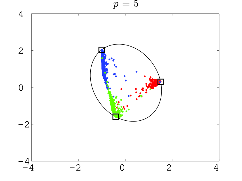
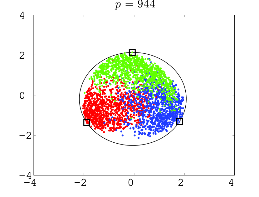
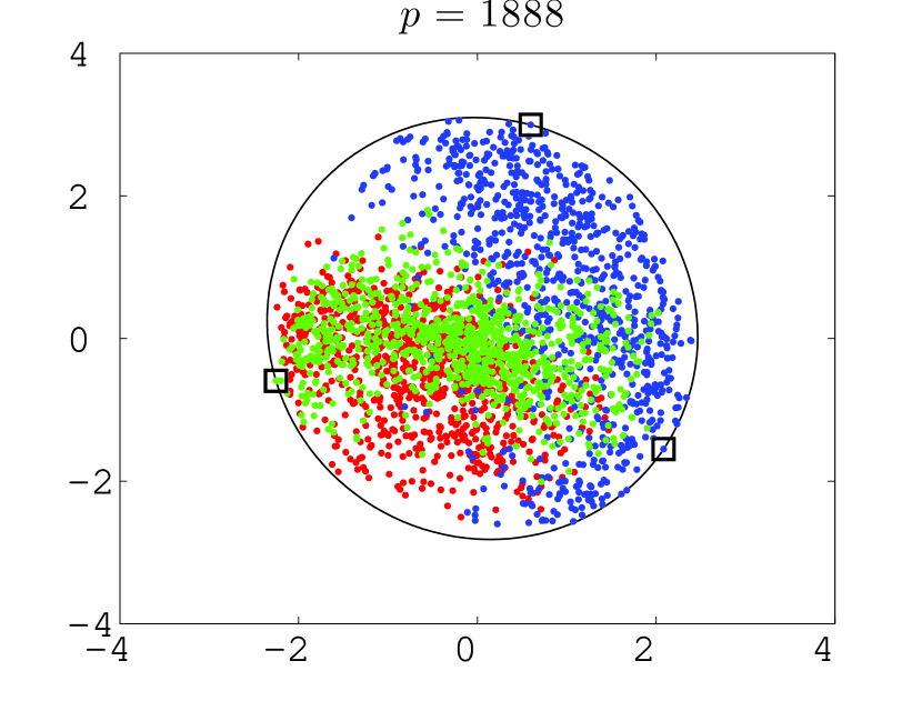
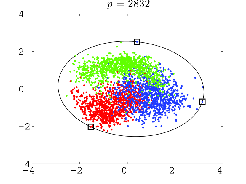
The clustering performance of NCER can be expected to be high if Observation 1 holds. Experiments were conducted with the purpose of illustrating this. We visualized the products produced by NCER on a small data set to see whether Observation 1 holds or not. The data set was constructed by picking image data in three classes of MNIST corresponding to handwritten digits 4, 5, and 6. The data set contained 2832 images of -by- pixels. We conducted NCER by using four different neighbor numbers , namely, and , chosen so as to divide the range from 0 to 2832 into three almost equal parts. The other input parameters were set such that is , and is the inner product of two data points.
Table 2 and Figure 2 display the experimental results. The table summarizes the ACs and NMIs for the four neighbor numbers. The figures may need some explanation. The size of the data matrix is -by-. The vectors constructed in the step 1 of NCER are -dimensional vectors due to and lie on a hyperplane . The MVEE for the set is -dimensional and is centrally symmetric, having the origin as the center. The figures show the intersections of and MVEE with . The figures display four cases for each neighbor number. The colored points correspond to , and red, blue and green respectively represent the three classes. The ellipsoids surrounded by the black lines are the MVEEs, and the squares surrounds active points.
| AC | 0.987 | 0.829 | 0.546 | 0.799 |
|---|---|---|---|---|
| NMI | 0.934 | 0.496 | 0.258 | 0.460 |
We can say from the figures that Observation 1 holds in the case of . We see from the table that the AC and NMI of this case are high. Meanwhile, it is difficult to say that Observation 1 holds in the other cases. In particular, the figure with displays that three types of data points are mixed and not separated. In fact, the AC and NMI of this case are low. We see from the figures with and that the data points group around three active points although some of the points are mixed. Hence, the ACs and NMIs of these cases are higher than those of .
7.3 Performance Evaluation
As mentioned in Section 5, the existing algorithms, NC, NMF, and GNMF, require the initial points to be chosen before they are run, and the choice affects the clustering performance. Hence, their performance may deteriorate with a choice of initial points which bring a low performance. Meanwhile, NCER does not have such issues. Hence, we can expect that its performance will be stable and as high as that of NC.
Experiments were conducted in the purpose of comparing the performance of NCER with the existing algorithms. In the experiments of the existing algorithms, we chose multiple initial points and measured the worst, best, and average performance. We randomly generated 100 initial points for running the K-means algorithm in NC and GNMF and 100 initial points for running the BCD framework to minimize the functions of (14) and (15) in NMF and GNMF. By using these initial points, we performed a total of 100 trials for each of NC and NMF and a total of 10000 trials for GNMF on each data set. Meanwhile, we carried out one trial for NCER on each data set. The parameters of NCER and NC were set such that is 5, is the number of classes in the data set, and is the inner product of two data points. We used the COIL20, JAFFE, ORL, MNIST, and USPS image data sets.
| NCER | NC | NMF | GNMF | ||||||||||
|---|---|---|---|---|---|---|---|---|---|---|---|---|---|
| ave | min | max | ave | min | max | ave | min | max | |||||
| COIL20 | 0.831 | 0.585 | 0.386 | 0.753 | 0.574 | 0.449 | 0.680 | 0.681 | 0.465 | 0.817 | |||
| JAFFE | 0.948 | 0.753 | 0.469 | 0.981 | 0.203 | 0.174 | 0.230 | 0.789 | 0.531 | 0.981 | |||
| ORL | 0.792 | 0.667 | 0.570 | 0.745 | 0.595 | 0.515 | 0.662 | 0.645 | 0.555 | 0.700 | |||
| MNIST | 0.663 | 0.664 | 0.500 | 0.810 | 0.522 | 0.429 | 0.532 | 0.632 | 0.449 | 0.727 | |||
| USPS | 0.802 | 0.710 | 0.395 | 0.937 | 0.683 | 0.563 | 0.756 | 0.750 | 0.289 | 0.940 | |||
| NCER | NC | NMF | GNMF | ||||||||||
|---|---|---|---|---|---|---|---|---|---|---|---|---|---|
| ave | min | max | ave | min | max | ave | min | max | |||||
| COIL20 | 0.933 | 0.813 | 0.695 | 0.887 | 0.712 | 0.666 | 0.748 | 0.857 | 0.774 | 0.919 | |||
| JAFFE | 0.938 | 0.874 | 0.721 | 0.974 | 0.109 | 0.068 | 0.141 | 0.910 | 0.794 | 0.974 | |||
| ORL | 0.875 | 0.837 | 0.787 | 0.869 | 0.788 | 0.759 | 0.811 | 0.825 | 0.797 | 0.842 | |||
| MNIST | 0.755 | 0.735 | 0.642 | 0.779 | 0.460 | 0.426 | 0.467 | 0.719 | 0.646 | 0.745 | |||
| USPS | 0.834 | 0.800 | 0.622 | 0.877 | 0.620 | 0.566 | 0.641 | 0.813 | 0.574 | 0.881 | |||
Tables 4 and 4 summarize the ACs and NMIs of the algorithms on each data set. Since multiple trials for NC, NMF, and GNMF were conducted, the statistics of the measurements are shown. The columns labeled “ave”, “min”, and “max” list the average, minimum, and maximum values of the corresponding measurements. For each data set, we compared the AC and NMI of NCER with the average ACs and NMIs of NC, NMF, and GNMF, and the tables show the highest values in boldface. We can see that the ACs and NMIs of NCER are higher than the average ACs and NMIs of the existing algorithms, except MNIST. NC and GNMF outperform NMF. For JAFFE and USPS, the maximum ACs and NMIs of NC and GNMF are higher than the ACs and NMIs of NCER, but their minimum ACs and NMIs are considerably lower than their maxima. Hence, the averages get worse. For COIL20 and ORL, we can also see that NC and GNMF have gaps between the minimum and maximum values of ACs and NMIs. For MNIST, although the AC of NCER is lower than the average AC of NC, the difference is quite small. Furthermore, the minimum AC of NC is lower than the AC of NCER. This indicates that there exists an initial point such that NC is inferior to NCER in AC. Consequently, we see that the performances of NC, NMF, and GNMF depend on the choice of the initial points and the average performance tends to get worse because some initial points result in poor performance. Meanwhile, NCER is a stable clustering algorithm and has high performance.
Let us mention the computational times of algorithms. The experiments showed that although the computational time of NCER is longer than that of NC, the difference is not so large. The biggest difference was in the case of USPS; NCER spent 81.4 seconds, while NC spent 67.0 seconds on average. It should be noted that the experimental results showed that the bottleneck in computational time is in solving the eigenvalue problem.
7.4 Connection of NCER with MER and ER
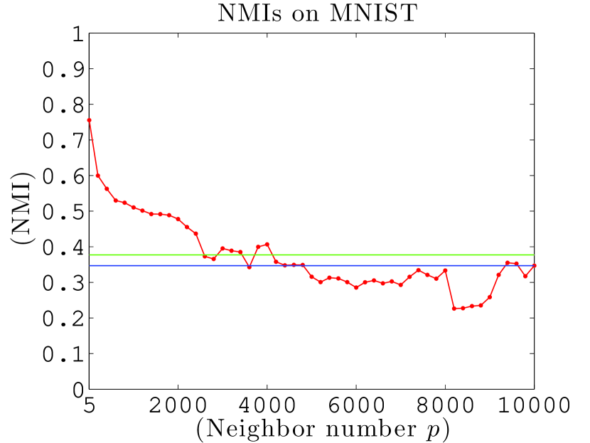
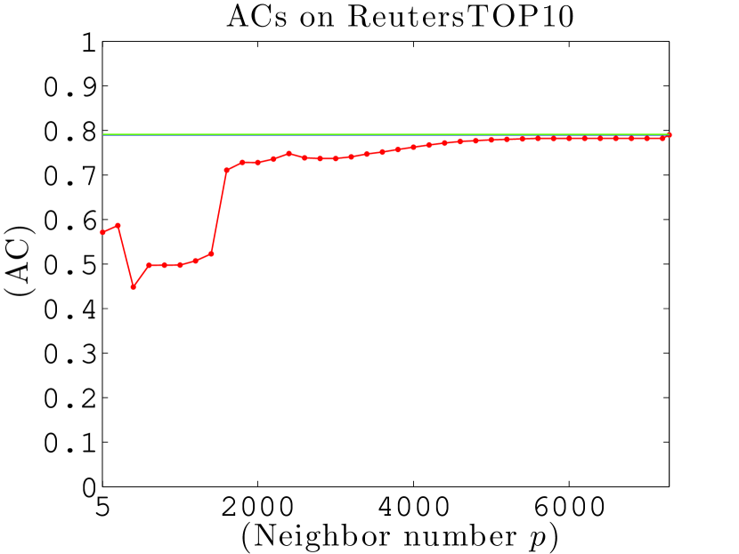
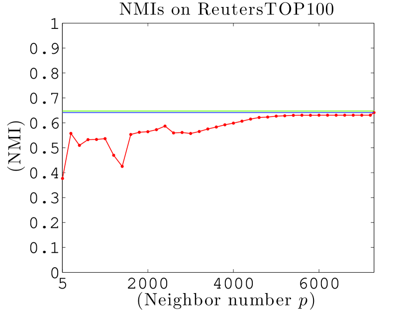
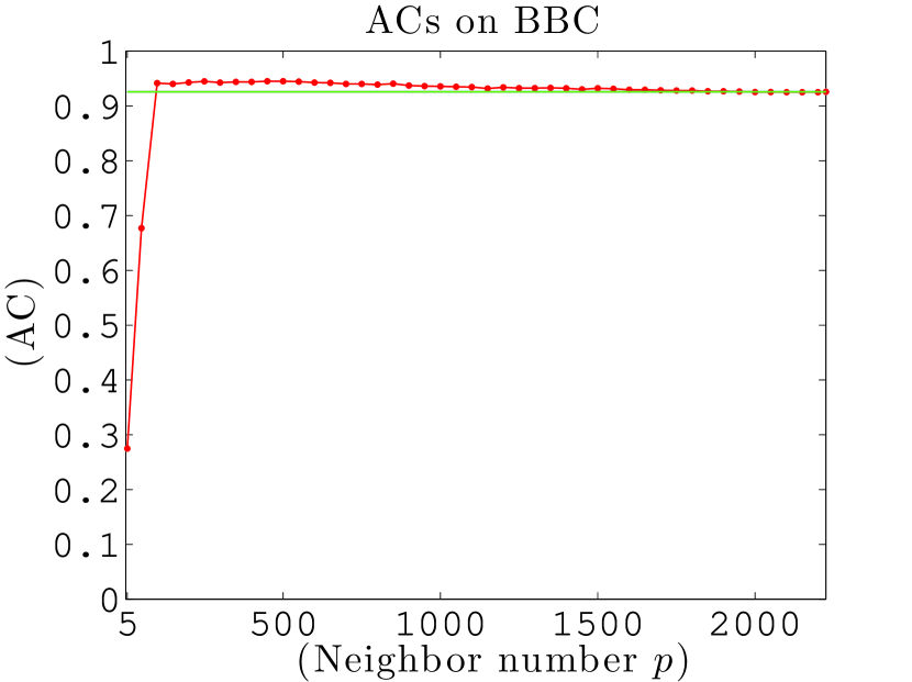
Finally, experiments were conducted to see how the performance of NCER varies with the neighbor number . We used the COIL20 and MNIST image data sets and the ReutersTOP10 and BBC document data sets.
We set the input parameters for NCER as follows. were chosen so as to increase by some unit size such that . Here, and are integers such that is strictly greater than and satisfies . The unit sizes of each data set were set as follows: on COIL20, on MNIST, on ReutersTOP10, and on BBC. The other input parameters were set such that is the number of classes in the data set, and is the inner product of two data points. We set the parameters for MER and ER as follows. Let be the matrix of (7). The data matrix was scaled to , and the scaled data matrix was used as the input for the algorithms. The matrix in step 2 of the algorithms was set as . The input parameter was chosen as the number of classes in a data set.
None of the data sets contained any data that corresponded to a zero vector, and the data matrices satisfied . Hence, Assumptions 2, 3, and 4 held when the neighbor number for NCER was set as . Accordingly, Theorem 1 and Corollary 1 ensured that, when , the clusters returned by NCER would not be far from those returned by ER and would coincide with those returned by MER.
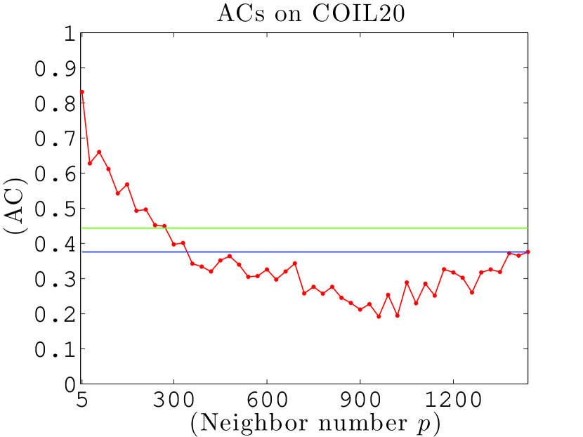
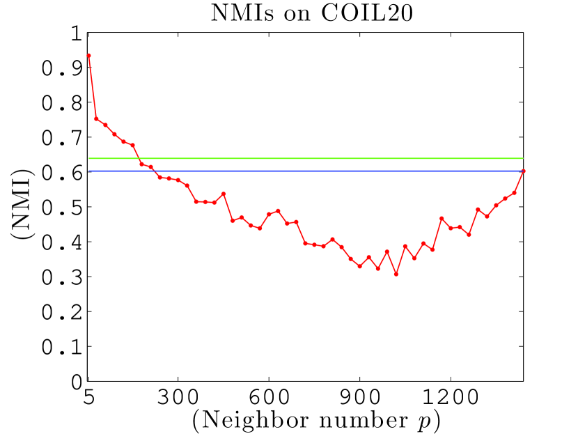
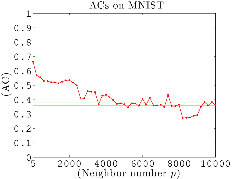
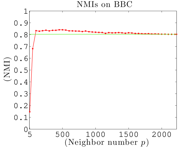
Figure 3 depicts the graphs for showing the ACs and NMIs of NCER, MER, and ER versus neighbor number . The red points connected by the red line plot the ACs and NMIs of NCER. The blue and green lines are the ACs and NMIs of MER and ER. Table 5 summarizes the ACs and NMIs of NCER with , MER, and ER. We can see from the figure and table that the ACs and NMIs of NCER coincide with those of MER when .
The graphs on the COIL20 and MNIST image data sets indicate that the clustering performance of NCER increases as the neighbor number gets close to zero. However, the graphs on the ReutersTOP10 and BBC document data sets indicate that the performance of NCER deteriorates when is a small number close to zero. This difference may have come from the differences in the degree of similarity in each class of the data sets. The data in the same class are quite similar to each other in the image data sets. For instance, regarding COIL20, the image data in a class were taken by turning an object through some interval of degrees. Thus, the image data in the same class may retain a similarity structure even as gets close to zero. However, this may not be the case in the document data sets, since the data in the same class are not as similar to each other as those of the image data sets.
| NCER with | MER | ER | ||||||
|---|---|---|---|---|---|---|---|---|
| AC | NMI | AC | NMI | AC | NMI | |||
| COIL20 | 0.376 | 0.602 | 0.376 | 0.602 | 0.444 | 0.639 | ||
| MNIST | 0.362 | 0.347 | 0.362 | 0.347 | 0.378 | 0.377 | ||
| ReutersTOP10 | 0.790 | 0.641 | 0.790 | 0.641 | 0.791 | 0.647 | ||
| BBC | 0.926 | 0.803 | 0.926 | 0.803 | 0.926 | 0.803 | ||
8 Concluding Remarks
We developed the NCER algorithm for spectral clustering; it is a variant of the normalized cut algorithm of Shi and Malik and Ng et al. The similarity with the ER algorithm for a separable NMF was discussed. In particular, if we modify one step of ER, the final outputs of NCER and the modified version of ER, called MER, coincide if we place assumptions on the data points and input parameters. Experiments indicated that NCER is a stable clustering algorithm and has high performance. They also showed how NCER behaves when the neighbor number was varied. The results confirmed our theoretical insight that NCER is connected with MER when is set to be equal to the number of data points.
Finally, we should mention the issues which will be addressed in future research. In the MVEE computation, we used a cutting plane framework to accelerate the efficiency of the interior-point algorithm. Thanks to the hybrid of interior-point algorithm and cutting plane algorithm, we could handle large problems. However, there is no theoretical guarantee that the hybrid algorithm terminates after a finite number of iterations. The experiments showed that it does not achieve the stopping criteria under some parameter settings even after many iterations. Therefore, we might want to consider alternative approaches for the computation. For instance, the conditional gradient algorithm, which is also referred to as the Frank-Wolfe algorithm, for the dual of MVEE formulation is a promising approach; [1] reports encouraging experimental results. The memory requirements of the algorithm are not so large, and thus, it should be able to work on large problems though it needs more iterations than the interior-point algorithm does.
References
- [1] S. D. Ahipasaoglu, P. Sun, and M. J. Todd. Linear convergence of a modified Frank-Wolfe algorithm for computing minimum-volume enclosing ellipsoids. Optimization Methods and Software, 23(1):5–19, 2008.
- [2] D. Aloise, A. Deshpande, P. Hansen, and P. Popat. NP-hardness of Euclidean sum-of-squares clustering. Machine Learning, 75(2):245–248, 2009.
- [3] S. Arora, R. Ge, Y. Halpern, D. Mimno, and A. Moitra. A practical algorithm for topic modeling with provable guarantees. In Proceedings of the 30th International Conference on Machine Learning (ICML), 2013.
- [4] S. Arora, R. Ge, R. Kannan, and A. Moitra. Computing a nonnegative matrix factorization – Provably. In Proceedings of the 44th symposium on Theory of Computing (STOC), pages 145–162, 2012.
- [5] S. Arora, R. Ge, and A. Moitra. Learning topic models – Going beyond SVD. In Proceedings of the 2012 IEEE 53rd Annual Symposium on Foundations of Computer Science (FOCS), pages 1–10, 2012.
- [6] S. Boyd and L. Vandenberghe. Convex Optimization. Cambridge University Press, 2004.
- [7] D. Cai, X. He, J. Han, and T. S. Huang. Graph regularized nonnegative matrix factorization for data representation. IEEE Transactions on Pattern Analysis and Machine Intelligence, 33(8):1548–1560, 2011.
- [8] C. Ding, X. He, and H. D. Simon. On the equivalence of nonnegative matrix factorization and spectral clustering. In Proceedings of the SIAM International Conference on Data Mining, pages 606–610, 2005.
- [9] P. Drineas, A. Frieze, R. Kannan, S. Vempala, and V. Vinay. Clustering large graphs via the singular value decomposition. Machine Learning, 56(1–4):9–33, 2004.
- [10] N. Gillis and S. A. Vavasis. Semidefinite programming based preconditioning for more robust near-spearable nonnegative matrix factorization. arXiv:1310.2273, 2013.
- [11] N. Gillis and S. A. Vavasis. Fast and robust recursive algorithms for separable nonnegative matrix factorization. IEEE Transactions on Pattern Analysis and Machine Intelligence, 36(4):698–714, 2014.
- [12] L. Hagen and A. B. Kahng. New spectral methods for ratio cut partitioning and clustering. IEEE Transactions on Computer-Aided Design, 11(9):1074–1085, 1992.
- [13] H. Kim and H. Park. Non-negative matrix factorization based on alternating non-negativity constrained least squares and active set method. SIAM Journal on Matrix Analysis and Applications, 30(2):713–730, 2008.
- [14] J. Kim, Y. He, and H. Park. Algorithms for nonnegative matrix and tensor factorizations: a unified view based on block coordinate descent framework. Journal of Global Optimization, 58(2):285–319, 2014.
- [15] A. Kumar, V. Sindhwani, and P. Kambadur. Fast conical hull algorithms for near-separable non-negative matrix factorization. In Proceedings of the 30th International Conference on Machine Learning (ICML), 2013.
- [16] C. L. Lawson and R. J. Hanson. Solving Least Squares Problems. Society for Industrial and Applied Mathematics, 1987.
- [17] D. D. Lee and H. S. Seung. Learning the parts of objects by non-negative matrix factorization. Nature, 401:788–791, 1999.
- [18] C.-J. Lin. Projected gradient methods for non-negative matrix factorization. Neural Computation, 19(10):2756–2779, 2007.
- [19] C. D. Manning, P. Raghavan, and H. Schuetze. Introduction to Information Retrieval. Cambridge University Press, 2008.
- [20] T. Mizutani. Ellipsoidal rounding for nonnegative matrix factorization under noisy separability. Journal of Machine Learning Research, 15:1011–1039, 2014.
- [21] A. Y. Ng, M. Jordan, and Y. Weiss. On spectral clustering: Analysis and an algorithm. In Advances in Neural Information Processing Systems 14 (NIPS), pages 849–856, 2001.
- [22] J. Shi and J. Malik. Normalized cuts and image segmentation. IEEE Transactions on Pattern Analysis and Machine Intelligence, 22(8):888–905, 2000.
- [23] P. Sun and R. M. Freund. Computation of minimum-volume covering ellipsoids. Operations Research, 52(5):690–706, 2004.
- [24] K.-C. Toh, M. J. Todd, and R. H. Tütüncü. SDPT3 – a MATLAB software package for semidefinite programming. Optimization Methods and Software, 11:545–581, 1999.
- [25] S. A. Vavasis. On the complexity of nonnegative matrix factorization. SIAM Journal of Optimization, 20(3):1364–1377, 2009.
- [26] U. von Luxburg. A tutorial on spectral clustering. Statistics and Computing, 17(4):395–416, 2007.
- [27] W. Xu, X. Liu, and Y. Gong. Document clustering based on non-negative matrix factorization. In Proceedings of the 26th annual international ACM SIGIR conference on Research and development in information retrieval (SIGIR), pages 267–273, 2003.