Local Expectation Gradients for Doubly Stochastic Variational Inference

Abstract

We introduce local expectation gradients which is a general purpose stochastic variational inference algorithm for constructing stochastic gradients through sampling from the variational distribution. This algorithm divides the problem of estimating the stochastic gradients over multiple variational parameters into smaller sub-tasks so that each sub-task exploits intelligently the information coming from the most relevant part of the variational distribution. This is achieved by performing an exact expectation over the single random variable that mostly correlates with the variational parameter of interest resulting in a Rao-Blackwellized estimate that has low variance and can work efficiently for both continuous and discrete random variables. Furthermore, the proposed algorithm has interesting similarities with Gibbs sampling but at the same time, unlike Gibbs sampling, it can be trivially parallelized.

1 Introduction

Stochastic variational inference has emerged as a promising and flexible framework for performing large scale approximate inference in complex probabilistic models. It significantly extends the traditional variational inference framework [4, 1] by incorporating stochastic approximation [10] into the optimization of the variational lower bound. Currently, there exists two major research directions in stochastic variational inference. The first attempts to deal with massive datasets by constructing stochastic gradients by using mini-batches of training examples [2, 3]. The second direction aims at dealing with the intractable expectations under the variational distribution that are encountered in non-conjugate probabilistic models [7, 8, 6, 11, 5, 9, 12]. The unified idea in the second direction is that stochastic optimization can be carried out by sampling from the variational distribution. This results in a doubly stochastic estimation approach, where the mini-batch source of stochasticity (the first direction above) can be combined with a second source of stochasticity associated with sampling from the variational distribution. Furthermore, within the second direction there exist now two main sub-classes of methods: the first based on the log derivative trick [7, 8, 6] and the second based on the reparametrization trick [5, 9, 12]. The first approach is completely general and can allow to apply stochastic optimization of variational lower bounds corresponding to arbitrary models and forms for the variational distribution. For instance, probabilistic models having both continuous and discrete latent variables can be accommodated by the log derivative trick approach. On the other hand, the reparametrization approach is specialised to continuous spaces and probabilistic models with differentiable joint distributions.

In this paper, we are interested to further investigate the doubly stochastic methods that sample from the variational distribution. A challenging issue here is concerned with the variance reduction of the stochastic gradients. Specifically, while the method based on the log derivative trick is the most general one, it has been observed to severely suffer from high variance problems [7, 8, 6] and thus it is only applicable together with sophisticated variance reduction techniques based on control variates. However, the construction of efficient control variates is a very challenging issue and in each application depends on the form of the probabilistic model. Therefore, it would be highly desirable to investigate whether it is possible to avoid using control variates altogether and construct simple stochastic gradient estimates that can work well for any probabilistic model. Notice, that while the reparametrization approach [5, 9, 12] has shown to perform well without the use of control variates, it is at the same time applicable only to a restricted class of variational inference problems that involve probabilistic models with differentiable joint distributions and variational distributions typically taken from the location-scale family.

Next, we introduce a general purpose algorithm for constructing stochastic gradients by sampling from the variational distribution that has a very low variance and can work efficiently without the need of any variance reduction technique. This method builds upon the log derivative trick and it is based on the key observation that stochastic gradient estimation over multiple variational parameters can be divided into smaller sub-tasks where each sub-task requires using more information coming from some part of the variational distribution and less information coming from other parts. For instance, assume we have a factorized variational distribution of the form $\prod_{i=1}^{n}q_{v_{i}}(x_{i})$ where $v_{i}$ is a local variational parameter and $x_{i}$ the associated latent variable. Clearly, $v_{i}$ determines the distribution over $x_{i}$, and therefore we expect the latent variable $x_{i}$ to be the most important piece of information for estimating $v_{i}$ or its gradient. Based on this intuitive observation we introduce the local expectation gradients algorithm that provides a stochastic gradient over $v_{i}$ by performing an exact expectation over the associated random variable $x_{i}$ while using a single sample from the remaining latent variables. Essentially this consist of a Rao-Blackwellized estimate that allows to dramatically reduce the variance of the stochastic gradient so that, for instance, for continuous spaces the new stochastic gradient is guaranteed to have lower variance than the stochastic gradient corresponding to the state of the art reparametrization method. Furthermore, the local expectation algorithm has striking similarities with Gibbs sampling with the important difference, that unlike Gibbs sampling, it can be trivially parallelized.

The remainder of the paper has as follows: Section 2 discusses the main two types of algorithms for stochastic variational inference that are based on simulating from the variational distribution. Section 3 describes the proposed local expectation gradients algorithm. Section 4 provides experimental results and the paper concludes with a discussion in Section 5.

2 Stochastic variational inference

Here, we discuss the main ideas behind current algorithms on stochastic variational inference and particularly doubly stochastic methods that sample from the variational distribution in order to approximate intractable expectations using Monte Carlo. Given a joint probability distribution $p(\mathbf{y},{{\bm{\mathbf{x}}}})$ where $\mathbf{y}$ are observations and ${{\bm{\mathbf{x}}}}$ are latent variables (possibly including model parameters that consist of random variables) and a variational distribution $q_{{{\bm{\mathbf{v}}}}}({{\bm{\mathbf{x}}}})$, the objective is to maximize the lower bound

$$F({{\bm{\mathbf{v}}}}) =\mathbbm{E}_{q_{{{\bm{\mathbf{v}}}}}({{\bm{\mathbf{x}}}})}\left[\log p(\mathbf{y},{{\bm{\mathbf{x}}}})-\log q_{{{\bm{\mathbf{v}}}}}({{\bm{\mathbf{x}}}})\right],$$ (1)

$$=\mathbbm{E}_{q_{{{\bm{\mathbf{v}}}}}({{\bm{\mathbf{x}}}})}\left[\log p(\mathbf{y},{{\bm{\mathbf{x}}}})\right]-\mathbbm{E}_{q_{{{\bm{\mathbf{v}}}}}({{\bm{\mathbf{x}}}})}\left[\log q_{{{\bm{\mathbf{v}}}}}({{\bm{\mathbf{x}}}})\right],$$ (2)

with respect to the variational parameters ${{\bm{\mathbf{v}}}}$. Ideally, in order to tune ${{\bm{\mathbf{v}}}}$ we would like to have a closed-form expression for the lower bound so that we could subsequently maximize it by using standard optimization routines such as gradient-based algorithms. However, for many probabilistic models and forms of the variational distribution at least one of the two expectations in (2) are intractable. For instance, if $p(\mathbf{y},{{\bm{\mathbf{x}}}})$ is defined though a neural network, the expectation $\mathbbm{E}_{q_{{{\bm{\mathbf{v}}}}}({{\bm{\mathbf{x}}}})}\left[\log p(\mathbf{y},{{\bm{\mathbf{x}}}})\right]$ will be analytically intractable despite the fact that $q_{{{\bm{\mathbf{v}}}}}({{\bm{\mathbf{x}}}})$ might have a very simple form, such as a Gaussian, so that the second expectation in eq. (2) (i.e. the entropy of $q_{{{\bm{\mathbf{v}}}}}({{\bm{\mathbf{v}}}})$) will be tractable. In other cases, such as when $q_{{{\bm{\mathbf{v}}}}}({{\bm{\mathbf{v}}}})$ is a mixture model or is defined through a complex graphical model, the entropic term will also be intractable. Therefore, in general we are facing with the following intractable expectation

$$\widetilde{F}({{\bm{\mathbf{v}}}})=\mathbbm{E}_{q_{{{\bm{\mathbf{v}}}}}({{\bm{\mathbf{x}}}})}\left[f({{\bm{\mathbf{x}}}})\right],$$ (3)

where $f({{\bm{\mathbf{x}}}})$ can be either $\log p(\mathbf{y},{{\bm{\mathbf{x}}}})$, $-\log q_{{{\bm{\mathbf{v}}}}}({{\bm{\mathbf{x}}}})$ or $\log p(\mathbf{y},{{\bm{\mathbf{x}}}})-\log q_{{{\bm{\mathbf{v}}}}}({{\bm{\mathbf{x}}}})$, from which we would like to efficiently estimate the gradient over ${{\bm{\mathbf{v}}}}$ in order to apply gradient-based optimization.

The most general method for estimating the gradient $\nabla_{{{\bm{\mathbf{v}}}}}\widetilde{F}({{\bm{\mathbf{v}}}})$ is based on the log derivative trick [7, 8, 6]. Specifically, this makes use of the property $\nabla_{{{\bm{\mathbf{v}}}}}q_{{{\bm{\mathbf{v}}}}}({{\bm{\mathbf{x}}}})=q_{{{\bm{\mathbf{v}}}}}({{\bm{\mathbf{x}}}})\nabla_{{{\bm{\mathbf{v}}}}}\log q_{{{\bm{\mathbf{v}}}}}({{\bm{\mathbf{x}}}})$, which allows to write the gradient as

$$\nabla_{{{\bm{\mathbf{v}}}}}\widetilde{F}({{\bm{\mathbf{v}}}})=\mathbbm{E}_{q_{{{\bm{\mathbf{v}}}}}({{\bm{\mathbf{x}}}})}\left[f({{\bm{\mathbf{x}}}})\nabla_{{{\bm{\mathbf{v}}}}}\log q_{{{\bm{\mathbf{v}}}}}({{\bm{\mathbf{x}}}})\right]$$ (4)

and then obtain an unbiased estimate according to

$$\frac{1}{S}\sum_{s=1}^{S}f({{\bm{\mathbf{x}}}}^{(s)})\nabla_{{{\bm{\mathbf{v}}}}}\log q_{{{\bm{\mathbf{v}}}}}({{\bm{\mathbf{x}}}}^{(s)}),$$ (5)

where each ${{\bm{\mathbf{x}}}}^{(s)}$ is an independent draw from $q_{{{\bm{\mathbf{v}}}}}({{\bm{\mathbf{x}}}})$. While this estimate is unbiased, it has been observed to severely suffer from high variance so that in practice it is necessary to consider variance reduction techniques such as those based on control variates [7, 8, 6]. Despite this limitation the above framework is very general as it can deal with any variational distribution over both discrete and continuous latent variables. The proposed method presented in Section 3 is essentially based on the log derivative trick, but it does not suffer from high variance.

The second approach is suitable for continuous spaces where $f({{\bm{\mathbf{x}}}})$ is a differentiable function of ${{\bm{\mathbf{x}}}}$ [5, 9, 12]. It is based on a simple transformation of (3) which allows to move the variational parameters ${{\bm{\mathbf{v}}}}$ inside $f({{\bm{\mathbf{x}}}})$ so that eventually the expectation is taken over a base distribution that does not depend on the variational parameters anymore. For example, if the variational distribution is the Gaussian $\mathcal{N}({{\bm{\mathbf{x}}}}|{{\bm{\mathbf{\mu}}}},LL^{\top})$ where ${{\bm{\mathbf{v}}}}=({{\bm{\mathbf{\mu}}}},L)$, the expectation in (3) can be re-written as $\widetilde{F}({{\bm{\mathbf{\mu}}}},L)=\int\mathcal{N}({{\bm{\mathbf{z}}}}|\mathbf{0},I)f({{\bm{\mathbf{\mu}}}}+L{{\bm{\mathbf{z}}}})d{{\bm{\mathbf{z}}}}$ and subsequently the gradient over $({{\bm{\mathbf{\mu}}}},L)$ can be approximated by the following unbiased Monte Carlo estimate

$$\frac{1}{S}\sum_{s=1}^{S}\nabla_{({{\bm{\mathbf{\mu}}}},L)}f({{\bm{\mathbf{\mu}}}}+L{{\bm{\mathbf{z}}}}^{(s)}),$$ (6)

where each ${{\bm{\mathbf{z}}}}^{(s)}$ is an independent sample from $\mathcal{N}({{\bm{\mathbf{z}}}}|\mathbf{0},I)$. This estimate makes efficient use of the slope of $f({{\bm{\mathbf{x}}}})$ which allows to perform informative moves in the space of $({{\bm{\mathbf{\mu}}}},L)$. For instance, observe that as $L\rightarrow 0$ the gradient over ${{\bm{\mathbf{\mu}}}}$ approaches $\nabla_{{{\bm{\mathbf{\mu}}}}}f({{\bm{\mathbf{\mu}}}})$ so that the optimization reduces to a standard gradient-ascent procedure for locating a mode of $f({{\bm{\mathbf{x}}}})$. Furthermore, it has been shown experimentally in several studies [5, 9, 12] that the estimate in (6) has relatively low variance and can lead to efficient optimization even when a single sample is used at each iteration. Nevertheless, a limitation of the approach is that it is only applicable to models where ${{\bm{\mathbf{x}}}}$ is continuous and $f({{\bm{\mathbf{x}}}})$ is differentiable. Even within this subset of models we are also additionally restricted to using certain classes of variational distributions [5, 9].

Therefore, it is clear that from the current literature is lacking a universal method that both can be applicable to a very broad class of models (in both discrete and continuous spaces) and also provide low-variance stochastic gradients. Next, we introduce such an approach..

3 Local expectation gradients

Suppose that the $n$-dimensional latent vector ${{\bm{\mathbf{x}}}}$ in the probabilistic model takes values in some space $\mathcal{S}_{1}\times\ldots\mathcal{S}_{n}$ where each set $\mathcal{S}_{i}$ can be continuous or discrete. We consider a variational distribution over ${{\bm{\mathbf{x}}}}$ that is represented as a directed graphical model having the following joint density

$$q_{{{\bm{\mathbf{v}}}}}({{\bm{\mathbf{x}}}})=\prod_{i=1}^{n}q_{v_{i}}(x_{i}|\text{pa}_{i}),$$ (7)

where $q_{v_{i}}(x_{i}|\text{pa}_{i})$ is the conditional factor over $x_{i}$ given the set of the parents denoted by $\text{pa}_{i}$. We assume that each conditional factor has its own separate set of variational parameters $v_{i}$ and ${{\bm{\mathbf{v}}}}=(v_{i},\ldots,v_{n})$. The objective is then to obtain a stochastic approximation for the gradient of the lower bound over each variational parameter $v_{i}$ based on the log derivative form in eq. (4).

Our method is motivated by the observation that each parameter $v_{i}$ is rather influenced mostly by its corresponding latent variable $x_{i}$ since $v_{i}$ determines the factor $q_{v_{i}}(x_{i}|\text{pa}_{i})$. Therefore, to get information about the gradient of $v_{i}$ we should be exploring multiple possible values of $x_{i}$ and a rather smaller set of values from the remaining latent variables ${{\bm{\mathbf{x}}}}_{\setminus i}$. Next we take this idea into the extreme where we will be using infinite draws from $x_{i}$ (i.e. essentially an exact expectation) together with just a single sample of ${{\bm{\mathbf{x}}}}_{\setminus i}$. More precisely, we factorize the variational distribution as follows

$$q_{{{\bm{\mathbf{v}}}}}({{\bm{\mathbf{x}}}})=q(x_{i}|\text{mb}_{i})q({{\bm{\mathbf{x}}}}_{\setminus i}),$$ (8)

where $\text{mb}_{i}$ denotes the Markov blanket of $x_{i}$. By using the log derivative trick the gradient over $v_{i}$ can be written as

$$\nabla_{v_{i}}\widetilde{F}({{\bm{\mathbf{v}}}}) =\mathbbm{E}_{q({{\bm{\mathbf{x}}}})}\left[f({{\bm{\mathbf{x}}}})\nabla_{v_{i}}\log q_{v_{i}}(x_{i}|\text{pa}_{i})\right],$$

$$=\mathbbm{E}_{q({{\bm{\mathbf{x}}}}_{\setminus i})}\left[\mathbbm{E}_{q(x_{i}|\text{mb}_{i})}\left[f({{\bm{\mathbf{x}}}})\nabla_{v_{i}}\log q_{v_{i}}(x_{i}|\text{pa}_{i})\right]\right],$$ (9)

where in the second expression we used the law of iterated expectations. Then, an unbiased stochastic gradient, say at the $t$-th iteration of an optimization algorithm, can be obtained by drawing a single sample ${{\bm{\mathbf{x}}}}_{\setminus i}^{(t)}$ from $q({{\bm{\mathbf{x}}}}_{\setminus i})$ so that

$$\mathbbm{E}_{q(x_{i}|\text{mb}_{i}^{(t)})}\left[f({{\bm{\mathbf{x}}}}_{\setminus i}^{(t)},x_{i})\nabla_{v_{i}}\log q_{v_{i}}(x_{i}|\text{pa}_{i}^{(t)})\right],$$ (10)

which is the expression for the proposed stochastic gradient for the parameter $v_{i}$. To get an independent sample ${{\bm{\mathbf{x}}}}_{\setminus i}^{(t)}$ from $q({{\bm{\mathbf{x}}}}_{\setminus i})$ we can simply simulate a full latent vector ${{\bm{\mathbf{x}}}}^{(t)}$ from $q_{{{\bm{\mathbf{v}}}}}({{\bm{\mathbf{x}}}})$ by applying the standard ancestral sampling procedure for directed graphical models [1]. Then, the sub-vector ${{\bm{\mathbf{x}}}}_{\setminus i}^{(t)}$ is by construction an independent draw from the marginal $q({{\bm{\mathbf{x}}}}_{\setminus i})$. Furthermore, the sample ${{\bm{\mathbf{x}}}}^{(t)}$ can be thought of as a pivot sample that is needed to be drawn once and then it can be re-used multiple times in order to compute all stochastic gradients for all variational parameters $v_{1},\ldots,v_{n}$ according to eq. (10).

When the variable $x_{i}$ takes discrete values, the expectation under $q(x_{i}|\text{mb}_{i}^{(t)})$ in eq. (10) reduces to a sum of terms associated with all possible values of $x_{i}$. On the other hand, when $x_{i}$ is a continuous variable the expectation in (10) corresponds to an univariate integral that in general may not be analytically tractable. In this case we shall use fast numerical integration methods (e.g. Gaussian quadrature when $q_{v_{i}}(x_{i}|\text{pa}_{i})$ is Gaussian).

We shall refer to the above algorithm for providing stochastic gradients over variational parameters as local expectation gradients and pseudo-code of a stochastic variational inference scheme that internally uses this algorithm is given in Algorithm 1. Notice that Algorithm 1 corresponds to the case where $f({{\bm{\mathbf{x}}}})=\log p(\mathbf{y},{{\bm{\mathbf{x}}}})-\log q_{{{\bm{\mathbf{v}}}}}({{\bm{\mathbf{x}}}})$ while other cases can be expressed similarly.

In the next two sections we discuss the computational complexity of the proposed algorithm and draw interesting connections between local expectation gradients with Gibbs sampling (Section 3.1) and the reparametrization approach for differentiable functions $f({{\bm{\mathbf{x}}}})$ (Section 3.2).

Algorithm 1 Stochastic variational inference using local expectation gradients

  Input: $f({{\bm{\mathbf{x}}}})$, $q_{{{\bm{\mathbf{v}}}}}({{\bm{\mathbf{x}}}})$.

  Initialize ${{\bm{\mathbf{v}}}}^{(0)}$, $t=0$.

  repeat

     Set $t=t+1$.

     Draw pivot sample ${{\bm{\mathbf{x}}}}^{(t)}\sim q_{{{\bm{\mathbf{v}}}}}({{\bm{\mathbf{x}}}})$.

     for $i=1$ to $n$ do

        $dv_{i}=\mathbbm{E}_{q(x_{i}|\text{mb}_{i}^{(t)})}\left[f({{\bm{\mathbf{x}}}}_{\setminus i}^{(t)},x_{i})\nabla_{v_{i}}\log q_{v_{i}}(x_{i}|\text{pa}_{i}^{(t)})\right]$.

        $v_{i}=v_{i}+\eta_{t}dv_{i}$.

     end for

  until convergence criterion is met.

3.1 Time complexity and connection with Gibbs sampling

In this section we discuss computational issues when running the proposed algorithm and we point out similarities and difference that has with Gibbs sampling.

Let us assume that time complexity is dominated by function evaluations of $f({{\bm{\mathbf{x}}}})$. We further assume that this function neither factorizes into a sum of local terms, where each term depends on a subset of variables, nor allows savings by performing incremental updates of statistics computed during intermediate steps when evaluating $f({{\bm{\mathbf{x}}}})$. Based on this the complexity per iteration is $O(nK)$ where $K$ is the maximum number of evaluations of $f({{\bm{\mathbf{x}}}})$ needed when estimating the gradient for each $v_{i}$. If each $x_{i}$ takes $K$ discrete values, the exact number of evaluations will be $n(K-1)+1$ where the “plus one” comes from the evaluation of the pivot sample ${{\bm{\mathbf{x}}}}^{(t)}$ that needs to be performed once and then it can be re-used for each $i=1,\ldots,n$. Notice that this time complexity corresponds to a worst-case scenario. In practice, we could save a lot of computations by taking advantage of any factorization in $f({{\bm{\mathbf{x}}}})$ and also the fact that any function evaluation is performed for inputs that are the same as the pivot sample ${{\bm{\mathbf{x}}}}^{(t)}$ but having a single variable changed. Furthermore, once we have drawn the pivot sample ${{\bm{\mathbf{x}}}}^{(t)}$ all function evaluations can be trivially parallelized.

There is an interesting connection between local expectation gradients and Gibbs sampling. In particular, carrying out Gibbs sampling in the variational distribution in eq. (7) requires iteratively sampling from each conditional $q(x_{i}|\text{mb}_{i})$, for $i=1,\ldots,n$. Clearly, the same conditional appears also in the local expectation algorithm when estimating the stochastic gradients. The obvious difference is that instead of sampling from $q(x_{i}|\text{mb}_{i})$ we now average under this distribution. Furthermore, for models having discrete latent variables the time complexity per iteration is the same as with Gibbs sampling with the important difference, however, that the algorithm of local expectation gradients is trivially parallelizable while Gibbs sampling is not.

3.2 Connection with the reparametrization approach

A very interesting property of local expectation gradients is that it is guaranteed to provide stochastic gradients having lower variance that the state of the art reparametrization method [5, 9, 12], also called stochastic belief propagation [9], which is suitable for continuous spaces and differential functions $f({{\bm{\mathbf{x}}}})$. Specifically, we will prove that this property holds for any factorized location-scale variational distribution of the form

$$q_{{{\bm{\mathbf{v}}}}}({{\bm{\mathbf{x}}}})=\prod_{i=1}^{n}q_{v_{i}}(x_{i}),$$ (11)

where $v_{i}=(\mu_{i},\ell_{i})$, $\mu_{i}$ is a location-mean parameter and $\ell_{i}$ is a scale parameter. Given that $q(z_{i})$ is the base distribution based on which we can reparametrize $x_{i}$ according to $x_{i}=\mu_{i}+\ell z_{i}$ with $z_{i}\sim q(z_{i})$, the single-sample stochastic gradient over $v_{i}$ is given by

$$\nabla_{v_{i}}f({{\bm{\mathbf{\mu}}}}+\bm{\ell}\circ{{\bm{\mathbf{z}}}}^{(t)}),\ \ z^{(t)}_{i}\sim q(z_{i}),$$ (12)

where ${{\bm{\mathbf{\mu}}}}$ is the vector of all $\mu_{i}$s, similarly $\bm{\ell}$ and ${{\bm{\mathbf{z}}}}^{(t)}$ are vectors of $\ell_{i}$s and $z_{i}^{(t)}$s, while $\circ$ denotes element-wise product. The local expectation stochastic gradient from eq. (10) takes the form

$$\int q_{v_{i}}(x_{i})f({{\bm{\mathbf{x}}}}_{\setminus i}^{(t)},x_{i})\nabla_{v_{i}}\log q_{v_{i}}(x_{i})dx_{i},$$

$$\int\nabla_{v_{i}}q_{v_{i}}(x_{i})f({{\bm{\mathbf{x}}}}_{\setminus i}^{(t)},x_{i})dx_{i}.$$ (13)

Now notice that ${{\bm{\mathbf{x}}}}_{\setminus i}^{(t)}={{\bm{\mathbf{\mu}}}}_{\setminus i}+\bm{\ell}_{\setminus i}\circ{{\bm{\mathbf{z}}}}_{\setminus i}^{(t)}$. Also by interchanging the order of the gradient and integral operators together with using the base distribution we have

$$\nabla_{v_{i}}\int q_{v_{i}}(x_{i})f({{\bm{\mathbf{\mu}}}}_{\setminus i}+\bm{\ell}_{\setminus i}\circ{{\bm{\mathbf{z}}}}_{\setminus i}^{(t)},x_{i})dx_{i},$$

$$=\nabla_{v_{i}}\int q(z_{i})f({{\bm{\mathbf{\mu}}}}+\bm{\ell}\circ{{\bm{\mathbf{z}}}}^{(t)})dz_{i},$$

$$=\int q(z_{i})\nabla_{v_{i}}f({{\bm{\mathbf{\mu}}}}+\bm{\ell}\circ{{\bm{\mathbf{z}}}}^{(t)})dz_{i},$$ (14)

where the final eq. (14) is clearly an expectation of the reparametrization gradient from eq. (12). Therefore, based on the standard Rao-Blackwellization argument the variance of the stochastic gradient obtained by (14) will always be lower or equal than the variance of the gradient of the reparametrization method. To intuitively understand this, observe that eq. (14) essentially says that the single-sample reparametrization gradient from (12) is just a Monte Carlo approximation to the local expectation stochastic gradient obtained by drawing a single sample from the base distribution, thus naturally it should have higher variance. In the experiments in Section 4 we typically observe that the variance provided by local expectation gradients is roughly one order of magnitude lower than the corresponding variance of the reparametrization gradients.

4 Experiments

In this section, we apply local expectation gradients (LeGrad) to different types of stochastic variational inference problems and we compare it against the standard stochastic gradient based on the log derivative trick (LdGrad) described by eq. (5) as well as the reparametrization-based gradient (ReGrad) given by eq. (6). In Section 4.1 we consider fitting using a factorized variational Gaussian distribution a highly correlated multivariate Gaussian. In Section 4.2, we consider a two-class classification problem using two digits from the MNIST database and we approximate a Bayesian logistic regression model using stochastic variational inference. Finally, in Section 4.3 we consider a sigmoid belief network with one layer of hidden variables and we fit it to the binarized version of the MNIST digits. For this problem we also parametrize the variational distribution using a recognition model.

4.1 Fitting a high dimensional Gaussian

We start with a simple “artificial” variational inference problem where we would like to fit a factorized variational Gaussian distribution of the form

$$q_{{{\bm{\mathbf{v}}}}}({{\bm{\mathbf{x}}}})=\prod_{i=1}^{n}\mathcal{N}(x_{i}|\mu_{i},\ell_{i}^{2}),$$ (15)

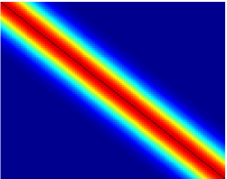
to a highly correlated multivariate Gaussian of the form $\mathcal{N}({{\bm{\mathbf{x}}}}|{{\bm{\mathbf{m}}}},\Sigma)$. We assume that $n=100$, ${{\bm{\mathbf{m}}}}=\bm{2}$, where $\bm{2}$ is the $100$-dimensional vector of $2$s. Further, the correlated matrix $\Sigma$ was constructed from a kernel function so that $\Sigma_{ij}=e^{-\frac{1}{2}(x_{i}-x_{j})^{2}}+0.1\delta_{ij}$ and where the inputs where placed in an uniform grid in $[0,10]$. This covariance matrix is shown in Figure 1. The smaller eigenvalue of $\Sigma$ is roughly $0.1$ so we expect that the optimal values for the variances $\ell_{i}^{2}$ to be around $0.1$ (see e.g. [1]) while the optimal value for each $\mu_{i}$ is $2$.

Given that the latent vector ${{\bm{\mathbf{x}}}}$ is continuous, to obtain the stochastic gradient for each $(\mu_{i},\ell_{i})$ we need to apply numerical integration. More precisely, the stochastic gradient for LeGrad according to eq. (10) reduces to an expectation under the Gaussian $\mathcal{N}(x_{i}|\mu_{i},\ell_{i}^{2})$ and therefore we can naturally apply Gaussian quadrature. We used the quadrature rule having $K=5$ grid points so that the whole complexity of LeGrad was $O(nK)=O(500)$ function evaluations per iteration (see Section 3.1). When we applied the standard LdGrad approach we set the number of samples in (5) equal to $S=500$ so that the computational costs of LeGrad and LdGrad match exactly with one another. When using the ReGrad approach based on (6) we construct the stochastic gradient using a single sample, as this is typical among the practitioners that use this method, and also because we want to empirically confirm the theory from Section 3.2 which states that the LeGrad method should always have lower variance than ReGrad given that the latter uses a sample size of one.

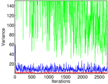
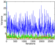
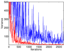
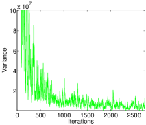
Figure 2(a) shows the evolution of the variance of the three alternative stochastic gradients (estimated by using the first variational parameter $\mu_{1}$ and a running window of $10$ previous iterations) as the stochastic optimization algorithm iterates. Clearly, LeGrad (red line) has the lowest variance, then comes ReGrad (blue line) and last is LdGrad which despite the fact that it uses $500$ independent samples in the Monte Carlo average in eq. (5) suffers from high variance. Someone could ask about how many samples the LdGrad method requires to decrease its variance to the level of the LeGrad method. In this example, we have found empirically that this is achieved when LdGrad uses $S=10^{4}$ samples; see Figure 2(b). This shows that LeGrad is significantly better than LdGrad and the same conclusion is supported from the experiment in Section 4.2 where we consider a Bayesian logistic regression model.

Furthermore, observe that the fact that LeGrad has lower variance than ReGrad is in a good accordance with the theoretical results of Section 3.2. Notice also that the variance of LeGrad is roughly one order of magnitude lower than the variance of ReGrad.

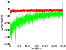
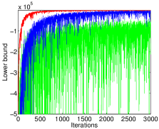
Finally, to visualize the convergence of the different algorithms and their ability to maximize the lower bound in Figure 2(c) we plot the stochastic value of the lower bound computed at each iteration by drawing a single sample from the variational distribution. Clearly, the stochastic value of the bound can allow us to quantify convergence and it could also be used as a diagnostic of high variance problems. From Figure 2(c) we can observe that LdGrad makes very slow progress in maximizing the bound while LeGrad and ReGrad converge rapidly.

Figure 1: The $100\times 100$ covariance matrix $\Sigma$ used in the experiment in Section 4.1.

(a)	(b)	(c)

Figure 2: The panel in (a) shows the variance of the gradient for the variational parameter $\mu_{1}$ when using LeGrad (red line), ReGrad (blue line) and LdGrad (green line). The number of samples used by LdGrad was $S=500$. The panel in (b) shows again the variances for all methods (the red and blue lines are from (a)) when LdGrad uses $S=10^{4}$ samples. The panel in (c) shows the evolution of the stochastic value of the lower bound (for LdGrad $S=500$ was used).

4.2 Logistic regression

In this section we compare the three approaches in a challenging binary classification problem using Bayesian logistic regression. We apply the stochastic variational algorithm in order to approximate the posterior over the regression parameters. Specifically, given a dataset $\mathcal{D}\equiv\{{{\bm{\mathbf{z}}}}_{j},y_{j}\}_{j=1}^{m}$, where ${{\bm{\mathbf{z}}}}_{m}\in\mathbbm{R}^{n}$ is the input and $y_{m}\in\{-1,+1\}$ the class label, we model the joint distribution over the observed labels and the parameters $\mathbf{w}$ by

$$p(\mathbf{y},\mathbf{w})=\left(\prod_{m=1}^{M}\sigma(y_{m}{{\bm{\mathbf{z}}}}_{m}^{\top}\mathbf{w})\right)p(\mathbf{w}),$$

where $\sigma(a)$ is the sigmoid function and $p(\mathbf{w})$ denotes a zero-mean Gaussian prior on the weights $\mathbf{w}$. As in the previous section we will assume a variational Gaussian distribution defined as in eq. (15) with the only notational difference that the unknowns now are model parameters, denoted by $\mathbf{w}$, and not latent variables.

For the above setting we considered a subset of the MNIST dataset that includes all $12660$ training examples from the digit classes $2$ and $7$. We applied all three stochastic gradient methods using a setup analogous to the one used in the previous section. In particular, the LeGrad method uses again a Gaussian quadrature rule of $K=5$ grid points so that the time complexity per iteration was $O(nK)=O(785*5)$ and where the number $785$ comes from the dimensionality of the digit images plus the bias term. To match this with the time complexity of LdGrad, we will use a size of $S=3925$ samples in the Monte Carlo approximation in eq. (5).

Figure 3(a) displays the variance of the stochastic gradient for the LeGrad method (green line) and the ReGrad method (blue line). As we can observe the local expectation method has roughly one order of magnitude lower variance than the reparametrization approach which is in a accordance with the results from the previous section (see Figure 2). In contrast to these two methods, which somehow have comparable variances, the LdGrad approach severely suffers from very high variance as shown in Figure 3(b) where the displayed values are of the order of $10^{7}$. Despite the fact that $3925$ independent samples are used in the Monte Carlo approximation still LdGrad cannot make good progress when maximizing the lower bound. To get a sensible performance with LdGrad we will need to increase considerably the sample-size which is computationally very expensive. Of course, control variates can be used to reduce variance to some extend, but it would have been much better if this problem was not present in the first place. LeGrad can be viewed as a certain variant of LdGrad but has the useful property that does not suffer from the high variance problem.

Finally, Figure 3(b) shows the evolution of the stochastic value of the lower bound for all three methods. Here, we can observe that LeGrad has significant faster and much more stable convergence than the other two methods. Furthermore, unlike in the example from the previous section, in this real dataset the ReGrad method exhibits clearly much slower convergence that the LeGrad approach.

Figure 3: The panel in (a) shows the variance of the gradient for the variational parameter $\mu_{1}$ when using LeGrad (red line), ReGrad (blue line), while panel (b) shows the corresponding curve for LdGrad (green line). The number of samples used by LdGrad was $S=3925$. The panel in (c) shows the evolution of the stochastic values of the lower bound.

Figure 4: The first row shows $100$ training examples and the learned model parameters $W$ for all $K=200$ hidden variables. The second row shows the corresponding reconstructed data and the evolution of the stochastic value of the lower bound.

4.3 Fitting one-layer sigmoid belief net with a recognition model

In the final example we consider a sigmoid belief network with a single hidden layer. More precisely, by assuming the observations are binary data vectors of the form $\mathbf{y}_{i}\in\{0,1\}^{D}$, such a sigmoid belief network assumes that each $\mathbf{y}_{i}$ is generated independently according to

$$p(\mathbf{y}|W)=\sum_{{{\bm{\mathbf{x}}}}}\prod_{d=1}^{D}\left[\sigma(\mathbf{w}_{d}^{\top}{{\bm{\mathbf{x}}}})\right]^{y_{d}}\left[1-\sigma(\mathbf{w}_{d}^{\top}{{\bm{\mathbf{x}}}})\right]^{1-y_{d}}p({{\bm{\mathbf{x}}}}),$$ (16)

where ${{\bm{\mathbf{x}}}}\in\{0,1\}^{K}$ is a vector of hidden variables while the prior $p({{\bm{\mathbf{x}}}})$ is taken to be uniform. The matrix $W$ (that incorporates also a bias term) consists of the set of model parameters to be estimated by fitting the model to the data. In theory we could use the EM algorithm to learn the parameters $W$, however, such an approach is not feasible because at the E step we need to compute the posterior distribution $p({{\bm{\mathbf{x}}}}_{i}|\mathbf{y}_{i},W)$ over each hidden variable which clearly is intractable since each ${{\bm{\mathbf{x}}}}_{i}$ takes $2^{K}$ values. Therefore, we need to apply approximate inference and next we consider stochastic variational inference using the local expectation gradients algorithm.

More precisely, by following recent trends in the literature for fitting this type of models [6, 5, 9] we assume a variational distribution parametrized by a “reverse” sigmoid network that predicts the latent vector ${{\bm{\mathbf{x}}}}_{i}$ from the associated observation $\mathbf{y}_{i}$:

$$q_{V}({{\bm{\mathbf{x}}}}_{i})=\prod_{k=1}^{K}\left[\sigma({{\bm{\mathbf{v}}}}_{k}^{\top}\mathbf{y}_{i})\right]^{x_{ik}}\left[1-\sigma({{\bm{\mathbf{v}}}}_{k}^{\top}\mathbf{y}_{i})\right]^{1-x_{ik}},$$ (17)

where $V$ is a matrix (that incorporates also a bias term) comprising the set of all variational parameters to be estimated. Often a variational distribution of the above form is referred to as the recognition model because allows to predict the activations of the hidden variables in unseen data $\mathbf{y}_{*}$ without needing to fit each time a new variational distribution.

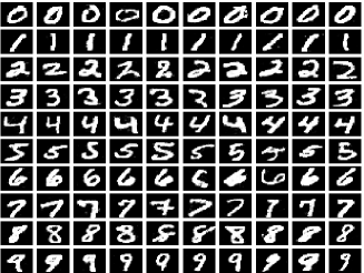
Based on the above model we considered a set of $1000$ binarized MNIST digits so that $100$ examples were chosen from each digit class. The application of stochastic variational inference is straightforward and boils down to constructing a separate lower bound for each pair $(\mathbf{y}_{i},{{\bm{\mathbf{x}}}}_{i})$ having the form

$$\mathcal{F}_{i}(V,W) =\sum_{{{\bm{\mathbf{x}}}}_{i}}q_{V}({{\bm{\mathbf{x}}}}_{i})\log\prod_{d=1}^{D}[\sigma(\mathbf{w}_{d}^{\top}{{\bm{\mathbf{x}}}}_{i})]^{y_{id}}[1-\sigma(\mathbf{w}_{d}^{\top}{{\bm{\mathbf{x}}}}_{i})]^{1-y_{id}}$$

$$-\sum_{k=1}^{K}\sigma({{\bm{\mathbf{v}}}}_{k}^{\top}\mathbf{y}_{i})\log\sigma({{\bm{\mathbf{v}}}}_{k}^{\top}\mathbf{y}_{i})-\sum_{k=1}^{K}(1-\sigma({{\bm{\mathbf{v}}}}_{k}^{\top}\mathbf{y}_{i}))\log(1-\sigma({{\bm{\mathbf{v}}}}_{k}^{\top}\mathbf{y}_{i})).$$ (18)

The total lower bound is then expressed as the sum of all data-specific bounds and it is maximized using stochastic updates to tune the forward model weights $W$ and the recognition weights $V$. Specifically, the update we used for $W$ was based on drawing a single sample from the full variational distribution: $q_{V}({{\bm{\mathbf{x}}}}_{i})$, with $i=1,\ldots,n$. The update for the recognition weights was carried out by computing the stochastic gradients according to the local expectation gradients so that for each ${{\bm{\mathbf{v}}}}_{k}$ the estimate obtained the following form

$$\nabla_{{{\bm{\mathbf{v}}}}_{k}}\mathcal{F}=\sum_{i=1}^{n}\nabla_{{{\bm{\mathbf{v}}}}_{k}}\mathcal{F}_{i} =\sum_{i=1}^{n}\sigma_{ik}(1-\sigma_{ik})\left[\sum_{d=1}^{D}\log\left(\frac{1+e^{-\widetilde{y}_{id}\mathbf{w}_{d}^{\top}({{\bm{\mathbf{x}}}}_{i\setminus k}^{(t)},x_{ik}=0)}}{1+e^{-\widetilde{y}_{id}\mathbf{w}_{d}^{\top}({{\bm{\mathbf{x}}}}_{i\setminus k}^{(t)},x_{ik}=1)}}\right)+\log\left(\frac{1-\sigma_{ik}}{\sigma_{ik}}\right)\right]\mathbf{y}_{i},$$ (19)

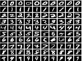
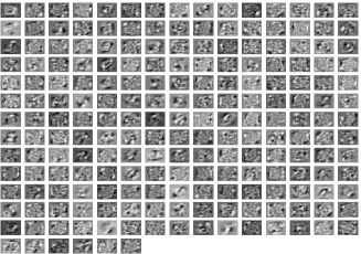
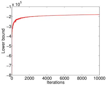
where $\sigma_{ik}=\sigma({{\bm{\mathbf{v}}}}_{k}^{\top}\mathbf{y}_{i})$ and $\widetilde{y}_{id}$ is the $\{-1,1\}$ encoding of $y_{id}$. Figure 4 shows several plots that illustrate how the model fits the data and how the algorithm converges. More precisely, we optimized the model assuming $K=200$ hidden variables in the hidden layer of the sigmoid network with the corresponding weights $W$ shown in Figure 4. Clearly, the model is able to provide very good reconstruction of the training data and exhibits also a fast and very stable convergence.

Finally, for comparison reasons we tried also to optimize the variational lower bound using the LdGrad algorithm. However, this proved to be very problematic since the algorithm was unable to make good progress and has severe tendency to get stuck to local maxima possibly due to the high variance problems.

5 Discussion

We have presented a stochastic variational inference algorithm which we call local expectation gradients. This algorithm provides a a general framework for estimating stochastic gradients that exploits the local independence structure of the variational distribution in order to efficiently optimize the variational parameters. We have shown that this algorithm does not suffer from high variance problems. Future work will concern with the further theoretical analysis of the properties of the algorithm as well as applications to hierarchical probabilistic models such as sigmoid belief networks with multiple layers.

References

- [1] Christopher M. Bishop. Pattern Recognition and Machine Learning. Springer, 2006.
- [2] Matthew D. Hoffman, David M. Blei, and Francis R. Bach. Online learning for latent dirichlet allocation. In NIPS, pages 856–864, 2010.
- [3] Matthew D. Hoffman, David M. Blei, Chong Wang, and John William Paisley. Stochastic variational inference. Journal of Machine Learning Research, 14(1):1303–1347, 2013.
- [4] Michael I. Jordan, Zoubin Ghahramani, Tommi S. Jaakkola, and Lawrence K. Saul. An introduction to variational methods for graphical models. Mach. Learn., 37(2):183–233, November 1999.
- [5] Diederik P. Kingma and Max Welling. Auto-encoding variational bayes. arXiv preprint arXiv:1312.6114, 2013.
- [6] Andriy Mnih and Karol Gregor. Neural variational inference and learning in belief networks. In The 31st International Conference on Machine Learning (ICML 2014), 2014.
- [7] John William Paisley, David M. Blei, and Michael I. Jordan. Variational bayesian inference with stochastic search. In ICML, 2012.
- [8] Rajesh Ranganath, Sean Gerrish, and David Blei. Black box variational inference. In Proceedings of the Seventeenth International Conference on Artificial Intelligence and Statistics (AISTATS), page 814–822, 2014.
- [9] Danilo Jimenez Rezende, Shakir Mohamed, and Daan Wierstra. Stochastic backpropagation and approximate inference in deep generative models. In The 31st International Conference on Machine Learning (ICML 2014), 2014.
- [10] Herbert Robbins and Sutton Monro. A Stochastic Approximation Method. The Annals of Mathematical Statistics, 22(3):400–407, 1951.
- [11] Tim Salimans and David A. Knowles. Fixed-form variational posterior approximation through stochastic linear regression. Bayesian Anal., 8(4):837–882, 12 2013.
- [12] Michalis K. Titsias and Miguel Lázaro-Gredilla. Doubly stochastic variational bayes for non-conjugate inference. In The 31st International Conference on Machine Learning (ICML 2014), 2014.