Abstract

Everyday we are exposed to various chemicals via food additives, cleaning and cosmetic products and medicines — and some of them might be toxic. However testing the toxicity of all existing compounds by biological experiments is neither financially nor logistically feasible. Therefore the government agencies NIH, EPA and FDA launched the Tox21 Data Challenge within the “Toxicology in the 21st Century” (Tox21) initiative. The goal of this challenge was to assess the performance of computational methods in predicting the toxicity of chemical compounds. State of the art toxicity prediction methods build upon specifically-designed chemical descriptors developed over decades. Though Deep Learning is new to the field and was never applied to toxicity prediction before, it clearly outperformed all other participating methods. In this application paper we show that deep nets automatically learn features resembling well-established toxicophores. In total, our Deep Learning approach won both of the panel-challenges (nuclear receptors and stress response) as well as the overall Grand Challenge, and thereby sets a new standard in tox prediction.

1 Introduction

Throughout their lives people are exposed to a sheer endless variety of chemical compounds, many of which are potentially dangerous. Determining the toxicity of a chemical is of crucial importance in order to minimize our exposure to harmful substances in every day products. Toxicity is also a central issue in the development of new drugs, with more than 30 % of drug candidates failing in clinical trials because of undetected toxic effects Kola & Landis (2004); Arrowsmith (2011).

In 2008, the U. S. National Institutes of Health (NIH) and the U. S. Environmental Protection Agency (EPA), agreed on collaborating on future toxicity testing activities Committee on Toxicity Testing and Assessment of Environmental Agents, National Research Council (2007). Their efforts were later joined by the U. S. Food and Drug Administration (FDA) under the umbrella of the Tox21 Program. The program’s stated goals are to develop better toxicity assessment methods, as current methods are not likely to scale with the increased demand for effective toxicity testing.

Current methods for testing the toxicity of a high number of chemicals rely on High-Throughput Screening (HTS). HTS experiments can investigate whether a chemical compound at a given concentration exhibits a certain type of toxicity, for a number of different compounds in parallel. These experiments are repeated with varying concentrations of the chemical compound, which allows to determine dose-response curves Inglese et al. (2006). From these curves one can reliably determine whether a compound activated a given pathway or receptor, inhibited it or did not interact at all.

Conducting these HTS experiments is a time- and cost-intensive process. Typically, a compound has to be tested for several types of toxicity at different concentration levels. Thus, the whole procedure has to be rerun for many times for each compound. Usually, a cell line has to be cultivated to obtain a single data point. Even an unprecedented multi-million-dollar effort, the Tox21 project, could test only a few thousands of compounds for as few as twelve toxic effects. Therefore, accurate computational methods for accurate prediction of toxic effects are highly demanded.

Existing computational approaches can be grouped into structure- and ligand-based. The structure-based methods simulate physical interactions between the compound and a biomolecular target (Kitchen et al., 2004) but are only applicable if the complete 3D structure of all interacting molecules are known, and they are infeasible for larger compound data bases. Ligand-based approaches predict the interactions based on previous measurements (Jenkins et al., 2007). Previous machine learning efforts were almost always ligand-based, such as scoring approaches like the Naive Bayes statistics (Xia et al., 2004; Nigsch et al., 2008; Mussa et al., 2013), density estimation (R. et al., 2012; Harper et al., 2001), nearest neighbor, support vector machines, and shallow feed forward neural networks  (Byvatov et al., 2003; Lowe et al., 2011).

In 2012, the Merck Kaggle challenge on chemical compound activity was won using deep neural networks, and the winning group later showed that multi-task learning can help to predict biological activities on single proteins Dahl et al. (2014). Dahl’s success inspired us to use Deep Learning for toxicity and target prediction Unterthiner et al. (2014). In contrast to biological activities of proteins, toxicological effects involve whole cell states determined by dysregulated biological processes. More specifically, toxicity prediction mainly focuses on cellular assays which measure cytotoxicity, i.e., they measure if a compound is toxic to a cell. A (cyto)toxic compound will cause harm to a cell, e.g. by causing acute mechanical injury or by triggering the programmed cell death mechanism (apoptosis) in the affected cells, which multicellular organisms use to protect themselves from cells that have gone out of control.

1.1 Deep Learning for Toxicity Prediction

Deep learning architectures seem to be well suited for toxicity prediction because they (1) automatically construct complex features Bengio et al. (2013) and (2) allow for multi-task learning Caruana (1997); Deng et al. (2013); Bengio et al. (2013).

One key aspect of toxicological research is its reliance on hierarchical levels of abstraction when thinking about chemical structures. A major research goal is the identification of toxicophores, Kier (1971); Lin (2000) which are the sets of steric and electronic properties that together produce a certain toxicological effect. These properties include hydrophobic regions, aromatic rings, electron acceptors or donors.

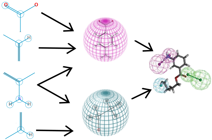
This maps naturally to Deep Learning architectures, where higher levels represent more complex concepts Bengio (2013). This idea is depicted in Figure 1, where ECFP4 input data (chemical substructures) represent low level properties in their first layer, which are combined to form reactive centers, which in turn encode toxicophores in higher layers.

Figure 1: Hierarchical nature of fingerprint features: by combining the ECFP features we can build reactive centers. By pooling specific reactive centers together we obtain a toxicophore that encodes a specific toxicological effect.

Additionally, Deep Learning is ideally suited for multi-task learning, which is a common setting for toxicology prediction: The same compound is often under investigation for several types of toxicity, and each of these types is its own prediction task. The work of Ramsundar et al. (2015) also shows that the multi-task environment does help when predicing chemical compounds, and that the performance boost obtained this way increases with the number of additional learning tasks. However, we typically have to deal with missing labels, as not all compounds will have been tested for each type of toxicity, or because some measurements were inconclusive.

Integrating all prediction tasks into one overarching multi-task setting offers two advantages: (a) it naturally allows for multi-label information and therefore can utilize relations between tasks; (b) it allows to share hidden unit representations among prediction tasks. The latter item is particularly important in our application as for some tasks very few measurements are available, therefore single-task prediction may fail to construct an effective representation. Thus, deep networks exploit representations learned across different tasks and can boost the performance on tasks with few training examples. Furthermore, this method allows us to predict an arbitrary number of toxicological effects at the same time, without the need to train single classifiers for each one.

2 Methods

2.1 DNN Architecture

Our system takes a numerical descriptor of a given compound as input, and tries to predict several different types of toxic effects at the same time. Such a type could be e.g. whether the compound acts as inhibitor to a specific nuclear receptor, or whether it activates a specific stress response pathway. Each of these types is a binary prediction task.

Formally, the problem we are trying to solve presents itself as follows: given a chemical compound $i$, we want to predict whether the compound has property $t$. We encode this information in the binary value $y_{it}$, where $y_{it}=1$ if the compound has the property and $y_{it}=0$ otherwise. We are interested in predicting the behavior of a compound on $T$ properties at the same time.

Each compound is represented using a number of numerical (or binary) features described later in this section. As training data, we are given a numerical representation $\mathbf{x_{i}}\in\mathbb{R}^{d}$ of $n$ training compounds as well as a sparsely populated matrix $\mathbf{Y}\in\mathbb{R}^{n\cdot m}$ of measurements.

We solve this by using a training objective that is the weighted sum of the cross-entropies over all tasks $t$:

$$-\sum_{t}^{T}m_{ti}\left(y_{it}\log\left(\sigma_{t}({\bf x_{i}})\right)+(1-y_{it})\log\left(1-\sigma_{t}({\bf x_{i}})\right)\right)$$

The binary variable $m_{ti}$ is 1 if sample $i$ has a valid label for task $t$ and 0 otherwise. Each single training sample contributed only to a few of the tasks. Thus, output units that were not active during a training sample were masked during backpropagation by multiplying their $\delta$ error by $m_{ti}$.

Our network consists of one or multiple layers of ReLU hidden units (Nair & Hinton, 2010; Glorot et al., 2011), followed by one layer of one or more sigmoid output units, one for each classification task.

2.2 Hyperparameters

The input features had substantially different scales and distributions, such that it was not obvious how to best preprocess them. We tried both the standard deviation as well as simple $\tanh$ nonlinearity to bring the chemical descriptors in the same range. ECFP4 features were either scaled by $tanh$ or sqrt nonlinearities. We additionally used a simple thresholding scheme to filter out very sparse features, which helped to bring the number of features down into a manageable range.

We tried different combinations of the available features, e.g. using only the binary ECFP4 fingerprints, or combining only the chemical descriptors with the toxicophore features.

To regularize our network, we used both Dropout Hinton et al. (2012); Srivastava et al. (2014) as well as small amounts of L2 weight decay, which both work in concert to avoid regularization  Krizhevsky et al. (2012); Dahl et al. (2014). Additionally, we used Early Stopping as determined via cross-validation.

Table 1 contains the complete list of hyperparameters we used for our network, as well as the search range for each parameter.

Hyperparameter	Considered values
Normalization	{standard-deviation, tanh, sqrt}
Feature type	{molecular-descriptors, tox-and-scaffold-similarities, ECFP4}
Fingerprint sparseness threshold	{5, 10, 20}
Number of Hidden Units	{1024, 4096, 8192, 16356}
Number of Layers	{1, 2, 3}
Learning Rate	{0.01, 0.05, 0.1}
Dropout	{no, yes (50% Hidden Dropout, 20% Input Dropout)}
L2 Weight Decay	{0, $10^{-6}$, $10^{-5}$, $10^{-4}$}

Table 1: Hyperparameters considered for the neural networks. Normalization: Scaling of the predefined features. Feature type: Determines which of the features were used as input features. “molecular-descriptors” were the real-valued descriptors. “tox-and-scaffold-similarities” were the similarity scores to known toxicophores and scaffolds, “ECFP4” were the ECFP4 fingerprint features. We tested all possible combinations of these features. Fingerprint sparseness threshold: A feature was not used if it was only present in fewer compounds than the given number. Number of hidden units: The number of units in the hidden layer of the neural network. Number of layers: The number of layers of the neural network. Learning rate: The learning rate for the backpropagation algorithm. Dropout: Dropout rates. L2 Weight Decay: The weight decay hyperparameter.

2.3 Input Features

Having good input features is a crucial issue for chemoinformatics applications. A vast variety of different methods exist, which calculate numerical features of the the typical graph-based storage format used for chemical compounds.

We used a high-dimensional binary representation using Extended Connectivity FingerPrint (ECFP4) features, the currently best performing compound description in drug design applications Rogers & Hahn (2010). Each feature/fingerprint denotes the presence-count of a certain chemical substructure, such as the ones given on the left-most column of Figure 1. In total, this produced approximately 30 000 very sparse features. As part of the hyperparameter selection we used a sparsity filter to emove non-informative ones.

We also calculated the similarity of each compound to 2 500 known toxicophore features, ie., patterns of substructures that were previously reported as toxicophores in the literature Kazius et al. (2005). We also calculated the similarity of each compound with 200 common chemical substructures that appear often in organic molecules.

Additionally, we calculated a number of descriptors based on the topological and physical properties of each compound. Typical descriptors for toxicity prediction can be grouped into 1D, 2D and 3D features Hong et al. (2008). Features that revolve around scalar properties such as counts of occurences for various atom-types, molecular weight or size are 1D features, while 2D features can be extracted from the planar chemical structure graph. These include graph-based features, 2D autocorrelation descriptors as well as van der Waals volume or the sum of Pauling atomic polarizabilities. Finally 3D structures usually involve force-field and quantum-mechanical simluations to extract things like solvent accessible surface area or partial charge informations.

We calculated a variety of these descriptors using off-the-shelf software Cao et al. (2013). However, not all descriptors could be calculated for all compounds. We used median-imputation to deal with missing values whenever feasible. This way we obtained a total of 5057 additional features.

2.4 Implementation

Depending on hyperparameter settings, our deep neural network had to deal with up to 40 000 input features and very large hidden layers. We stored the weight parameters on a single GPU with 12 GB RAM and used mini-batches of 512 samples for stochastic gradient descent learning. Since storing our input data in dense format requires about 5 TB of disk space, we used a sparse storage format. However, it proved to be faster to upload a mini-batch in sparse format to the GPU and then convert it to dense format instead of using sparse matrix multiplication.

3 Experimental Results

3.1 Tox21 Data Challenge Data

We validated our approach using the data from the Tox21 Data Challenge National Center for Advancing Translational Sciences (2014), a toxicity prediction challenge organized by the Tox21 program partners open to participants worldwide. The data for this challenge was collected within the framework of the Tox21 research initiative, which aims to produce highly realiable measurements with stringent quality-control criteria, that are otherwise hard to come by in public databases.

The data set provided by the Tox21 Data Challenge included approximately 12 000 compounds and was composed of twelve different sub-challenges/tasks. Each sub-challenge required the prediction of a different type of toxicity. The sub-challenges were split between two panels: Seven of the twelve sub-challenges dealt with Nuclear Receptor (NR) signaling pathways, the remaining five with the Stress Response (SR) pathways.

Nuclear receptors are important components in cell communication and control, and are involved in development, metabolism and proliferation. They have been shown to play a key role in toxicology as well Woods et al. (2007). The Tox21 data set investigated several NRs involved in endocrine system, i.e., the secretion of hormones into the blood stream, as toxins can cause disruption of the normal endocrine function. Two such nuclear hormone receptors, the estrogen and the androgen receptor, have been measured by two independent systems, once using a luminescence method, and once using a modified antibiotic resistance gene (NR.ER and NR.ER.LBD / NR.AR and NR.AR.LBD respectively). Furthermore, the challenge included a task on predicting the antagonists of the aromatase enzyme, which catalyzes the conversion of androgen to estrogen and thereby keeps the balance between these two hormones (NR.Aromatase). The last two NRs in the Tox21 data set were the aryl hydrocarbon receptor (NR.AhR) which is essential for reacting to a cell’s environmental changes, and a specific subtype of the peroxisome proliferator-activated receptors (NR.PPAR.gamma) which is involved in the regulation of various genes as well as metabolism. Overall the NR tasks included a broad variety of different toxicity-related receptors.

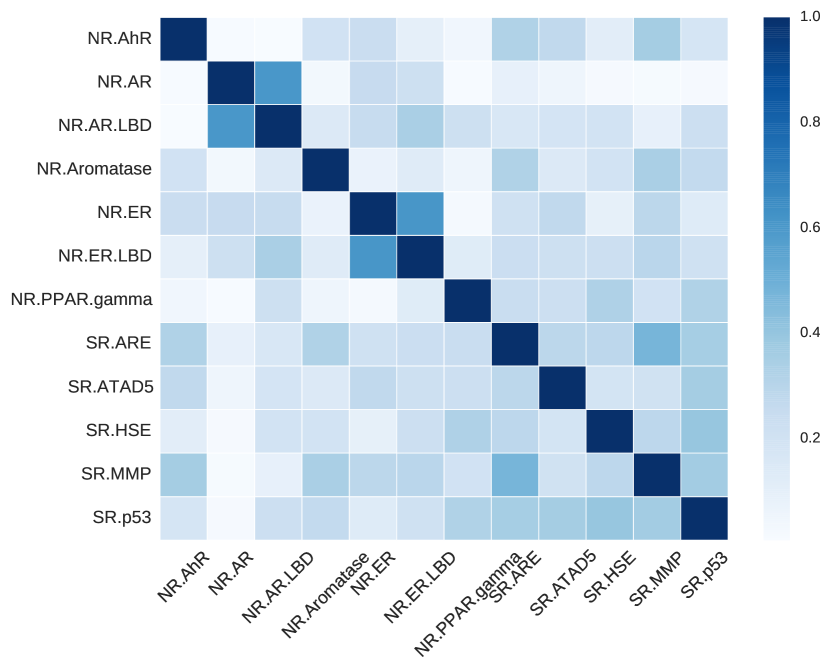
Toxicity can also cause cellular stress which in term can lead to apoptosis. Therefore the Tox21 data also includes five tasks on various stress response indicators: The antioxidant response element signaling pathway (SR.ARE) directly reacts to oxidative stress, while the heat shock factor response element (SR.HSE) is involved in reacting to heat shocks as part of the cell’s internal repair mechanisms. The ATAD5 signaling pathway will be activated when a cell detects DNA damage (SR.ATAD5). The SR panel also includes a task on predicting which compounds influence the mitochondrial membrane potential (SR.MMP), which is essential for generating the energy a cell consumes. Finally, the p53 task requires participants to detect activation of the p53 pathway (SR.p53), a well known cancer pathway which is activated both by DNA damage, but also reacts to various other cellular stresses. For this reason, a compound that triggers any of the other stress response pathways has a high probability to also show up as active on the p53 task. In general, all of the SR tasks show higher correlation with each other than the nuclear receptor tasks (c.f. Figure 3).

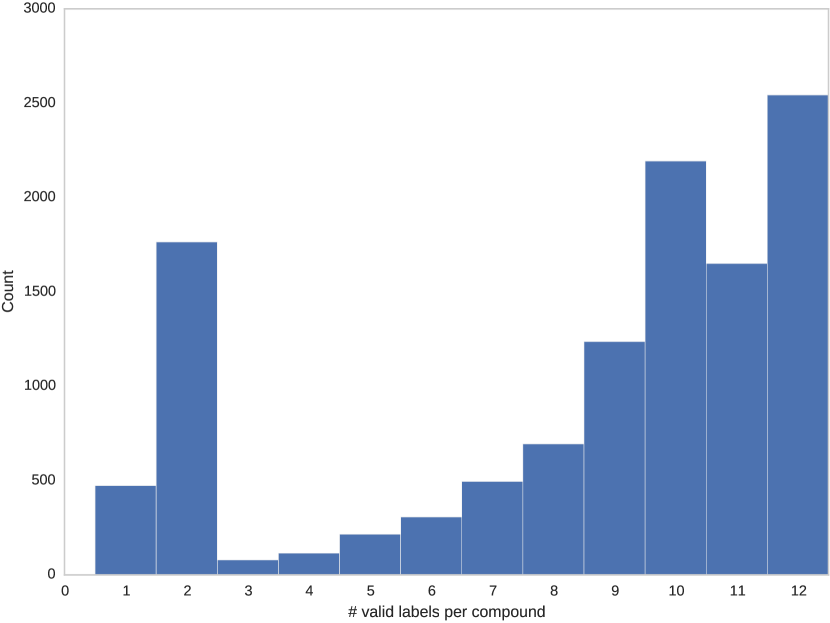
Most of the compounds were measured on several of the tasks (c.f. Figure 2), such that all the tasks operated on subsets of the same overall data set. This allowed us to compute correlations between the tasks, displayed in Figure 3. As expected, the tasks that involved measuring the same pathway via different methods (AR/AR-LBD and ER/ER-LBD) were highly correlated. Also, the p53 pathway, which is one of the main focal points of stress response signaling, showed high levels of correlation with the other tasks that measured specific stress responses.

Overall, the compounds were split into a training set consisting of 11 764 compounds with known labels, a leaderboard set used to rank participants on a public leaderboard (297 compounds) as well as a private test set used for the final evaluation of all submitted entries (643 compounds). The labels for the leaderboard set were initially held back, but later made available to the participants in the final stages of the competition, while the labels of the final test set have not yet been released.

Figure 2: Number of tasks each training compound of the Tox21 Data Challenge was part of. Only $\approx 500$ compounds were part of only a single task, with over half (54 %) of the compounds being labeled in 10 or more of the tasks.

Figure 3: Absolute correlation coefficient between the different tasks of the Tox21 Data Challenge

Task	AUC ST	AUC MT	$p$-value
NR.AhR	0.8487	0.8409	0.072
NR.AR	0.3755	0.3459	0.202
NR.AR.LBD	0.8799	0.9289	0.011
NR.Aromatase	0.7523	0.7921	0.006
NR.ER	0.6659	0.6949	0.006
NR.ER.LBD	0.6532	0.7272	0.006
NR.PPAR.gamma	0.6367	0.7102	0.006
SR.ARE	0.7927	0.8017	0.148
SR.ATAD5	0.7972	0.7958	0.338
SR.HSE	0.7354	0.8101	0.006
SR.MMP	0.8485	0.8489	0.265
SR.p53	0.6955	0.7487	0.006

Table 2: Comparing single-task (ST) and multi-task (MT) learning. Evaluation was done on the Tox21 leaderboard set. Results are the mean values of training 5 nets from different random initializations. Significant differences according to a two-sided Mann - Whitney U test in bold.

3.1.1 Data Preprocessing

The Tox21 training set contains redundant compounds that appear multiple times within the data, but each time accompanied by carrier molecules such as water, salts or other solubles. Also, we observed compounds that actually consisted of two unrelated structures, but which for some unknown reason where encoded together. We semi-automatically labeled these fragments, cleaning up contradictory and combining agreeing compounds. This way we identified 8,695 distinct compound fragments.

To further clean up the data, we made ran a standard clean-up routine for chemical compounds on the data using ChemAxon. This made all hydrogen atoms explicit, ensured that aromatic bonds and tautomers where coded consistently and unified the encoding of salts. We then calculated the input features as described in subsection 2.3.

 
 

Figure 4: Neurons that have learned to detect the presence of pharmacophores. Each row shows a certain hidden unit in a learned network that correlates highly with a certain toxicophore feature. The row shows the three chemical compounds that had the highest activation for that neuron. Emphasized in red is the toxicophore structure from the literature that the neuron correlates with. Rows 1 and 2 are from the first hidden layer, the last row is from a higher layer.

3.2 Evaluation

We defined cross-validation sets for hyperparameter selection, optimizing for two goals: a) The class-distributions should be close to the final test set. In the training set many compounds were only measured on a small subset of assay, whereas we expected compounds in the final test set to be labeled on all twelve tasks. We therefore included only compounds that were labeled on at least eight tasks in the cross-validation sets. The remaining, sparsely labeled compounds were added to the training set of each fold. b) The cross-validation sets should not be overly simple. We wanted to avoid the situation where the training samples were exceedingly similar to the test samples. This happens frequently within chemical data because a number of compounds might share the same chemical backbone. Therefore, we clustered the compounds according to their structural similarity Verbist et al. (2015) and distributed the resulting clusters among the five cross-validation folds.

We used the AUC score as quality criterion, which we optimized independently for each task. So even though we employed multi-task networks, we optimized the hyperparameters differently for each task at hand.

3.3 Multitask Learning

Most of the compounds where labeled on several of the tasks (c.f. Figure 2), which allowed us to calculate the correlation between different tasks. As can be seen in Figure 3, the twelve different task of the Tox21 Data Challenge Data were highly correlated with one another. Thus, this was an ideal setting for multi-task learning.

To see whether multi-task learning really helps in this scenario as much as it did when predicting biological activities on protein level Dahl et al. (2014), we also trained single-task neural networks on the same tasks.

As shown in Table 2, in almost all tasks the multi-task learning approach significantly outperforms the single task networks. Both networks failed in one task which suffered from very unbalanced class distribution (only 3 positive examples in the leaderboard set).

3.4 Learning Toxicophore Representation

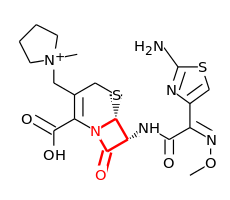
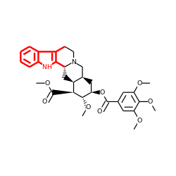
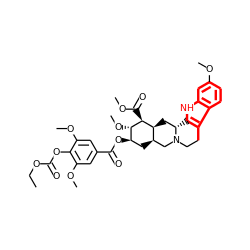
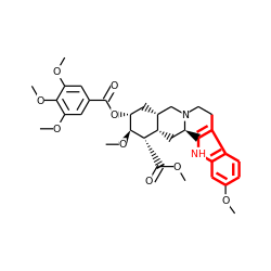
One of the hallmarks of Deep Learning are several layers of hierarchical representations of increasing abstractions Bengio et al. (2013). Within the chemical research community such a hierarchy of features has naturally emerged: single atoms are grouped together as functional groups and reactive centers, which in turn define toxicophores (c.f. Figure 1. Such features are the state-of-the-art way that chemists and drug designers think about the properties of each chemical compound Kazius et al. (2005). To determine the effectiveness of Deep Learning for toxicity prediction, we investigated whether the network did implicitly encode toxicophore features in its hidden layers.

We trained a multi-task deep network on the Tox21 data using exclusively ECFP4 fingerprint-features as input. Each fingerprint encodes how many times a specific, small chemical substructure appears within a compound. No other input features were used.

After training, we computed the correlation between the activations of the hidden units and the presence/absence of known toxicophore features in the compounds. We did indeed find several highly significant correlations, clearly demonstrating that the hidden units of a neural network do indeed automatically learn toxicophore structures.

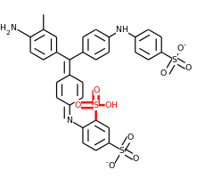
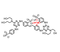
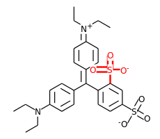
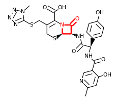
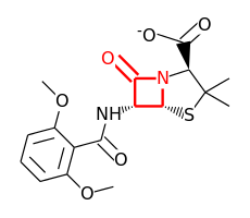
Visual inspection of the results showed that lower layers did tend to learn smaller features, often focusing on single functional groups like e.g. sulfonyl-groups (see row 1 and 2 of Figure 4, while in higher layers the correlations were more with larger toxicophore clusters, even involving structures that did not match the toxicophore perfectly (row 3 of Figure 4.

4 Results

The Tox21 Data Challenge Data attracted a large crowd of participants from all over the world, including submissions from leading research labs and industry.

The final evaluation was done by the organizers on a held back evaluation set consisting of 643 compounds. The teams were allowed to send in predictions for these final compounds, but did not receive any feedback as to how well they fared. The final scoring on each sub-challenge was based on the AUC values of each team’s final submission.

	AVG	NR	SR	AhR	AR	AR-LBD	ARE	Aromatase	ATAD5	ER	ER-LBD	HSE	MMP	p53	PPAR.g
our method	gray!350.846	gray!350.826	gray!350.858	gray!350.928	gray!200.807	gray!350.850	gray!350.840	gray!200.834	0.793	gray!200.793	gray!200.814	gray!200.858	0.941	gray!200.862	gray!350.839
AMAZIZ	gray!200.838	gray!200.816	gray!200.854	gray!200.913	0.770	0.846	gray!200.805	0.819	gray!350.828	gray!350.806	0.806	0.842	gray!350.950	0.843	0.830
dmlab	0.824	0.811	0.850	0.781	gray!350.828	0.819	0.768	gray!350.838	0.800	0.766	0.772	0.855	gray!200.946	gray!350.880	gray!200.831
T	0.823	0.798	0.842	0.913	0.676	gray!200.848	0.801	0.825	gray!200.814	0.784	0.805	0.811	0.937	0.847	0.822
microsomes	0.810	0.785	0.814	0.901	–	–	0.804	–	0.812	0.785	gray!350.827	–	–	0.826	0.717
filipsPL	0.798	0.765	0.817	0.893	0.736	0.743	0.758	0.776	–	0.771	–	0.766	0.928	0.815	–
Charite	0.785	0.750	0.811	0.896	0.688	0.789	0.739	0.781	0.751	0.707	0.798	0.852	0.880	0.834	0.700
RCC	0.772	0.751	0.781	0.872	0.763	0.747	0.761	0.792	0.673	0.781	0.762	0.755	0.920	0.795	0.637
frozenarm	0.771	0.759	0.768	0.865	0.744	0.722	0.700	0.740	0.726	0.745	0.790	0.752	0.859	0.803	0.803
ToxFit	0.763	0.753	0.756	0.862	0.744	0.757	0.697	0.738	0.729	0.729	0.752	0.689	0.862	0.803	0.791
CGL	0.759	0.720	0.791	0.866	0.742	0.566	0.747	0.749	0.737	0.759	0.727	0.775	0.880	0.817	0.738
SuperTox	0.743	0.682	0.768	0.854	–	0.560	0.711	0.742	–	–	–	–	0.862	0.732	–
kibutz	0.741	0.731	0.731	0.865	0.750	0.694	0.708	0.729	0.737	0.757	0.779	0.587	0.838	0.787	0.666
MML	0.734	0.700	0.753	0.871	0.693	0.660	0.701	0.709	0.749	0.750	0.710	0.647	0.854	0.815	0.645
NCI	0.717	0.651	0.791	0.812	0.628	0.592	0.783	0.698	0.714	0.483	0.703	gray!350.858	0.851	0.747	0.736
VIF	0.708	0.702	0.692	0.827	0.797	0.610	0.636	0.671	0.656	0.732	0.735	0.723	0.796	0.648	0.666
Toxic Avg	0.644	0.659	0.607	0.715	0.721	0.611	0.633	0.671	0.593	0.646	0.640	0.465	0.732	0.614	0.682
Swamidass	0.576	0.596	0.593	0.353	0.571	0.748	0.372	0.274	0.391	0.680	0.738	0.711	0.828	0.661	0.585

Table 3: Results of the leading teams in the Tox21 Data Challenge, best results in bold and gray background, second best results in light gray. AVG is the average over all 12 subchallenges. NR/SR are averages over all tasks that are part of the “Nuclear Receptor” and “Stress Response” panels, respectively. The left side shows the individual sub-challenges. Team-names have been abbreviated in order to save space. The full list of results is available online at https://tripod.nih.gov/tox21/challenge/leaderboard.jsp.

Our approach which was spearheaded by the deep neural network presented in this paper showed the most consistent performance of all participants: It never placed lower than fifth place in any of the tasks, and outright won a total of 8 of the 15 challenges. In particular, it achieved the best average AUC in both the SR and NR panels, as well as as well as the best average AUC over the whole set of sub-challenges. It was thus declared winner of both the Nuclear Receptor and the Stress Response pannel, as well as the overall Tox21 Grand Challenge. The detailed results are displayed in Table 3.

5 Conclusion

In this paper we applied of deep neural networks to toxicity prediction. We showed that deep networks are able to learn a highly effective representation of chemical compounds. In this representation we could detect toxicophores, proven concepts which have previously often been handcrafted over decades by experts in the field. It stands to reason that these representations also include novel, previously undiscovered toxicophores that are lying dormant in the data. Using these representations, our approach outperformed methods that were specifically tailored for toxicological applications.

As demonstrated by the Tox21 Data Challenge, our method sets a new state of the art in this field. As the NIH confirmed National Center for Advancing Translational Sciences (2015), the high quality of the models makes them suitable for deployment in leading edge toxicological research. We believe that Deep Learning has the ability to greatly influence the field of toxicity prediction in the future. Toxicology is a crucial part of modern environmental health, drug development and pharmaceutical research, and machine learning is on the verge of becoming a vital part of it.

References

- Arrowsmith (2011) Arrowsmith, J. Trial watch: phase III and submission failures: 2007–2010. Nature Reviews Drug Discovery, 10(2):87–87, 2011.
- Bengio (2013) Bengio, Y. Deep learning of representations: Looking forward. In Proceedings of the First International Conference on Statistical Language and Speech Processing, SLSP’13, pp. 1–37, Berlin, Heidelberg, 2013. Springer-Verlag. ISBN 978-3-642-39592-5.
- Bengio et al. (2013) Bengio, Y., Courville, A., and Vincent, P. Representation learning: A review and new perspectives. IEEE Trans Pattern Anal Mach Intell, Feb 2013.
- Byvatov et al. (2003) Byvatov, E., Fechner, U., Sadowski, J., and Schneider, G. Comparison of Support Vector Machine and Artificial Neural Network Systems for Drug/Nondrug Classification. Journal of Chemical Information and Computer Sciences, 43(6):1882–1889, September 2003.
- Cao et al. (2013) Cao, DS., Xu, QS., Hu, QN., and Liang, YZ. ChemoPy: freely available python package for computational biology and chemoinformatics. Bioinformatics, 29(8):1092–1094, 2013.
- Caruana (1997) Caruana, R. Multitask learning. Machine Learning, 28(1):41–75, 1997. ISSN 0885-6125.
- Committee on Toxicity Testing and Assessment of Environmental Agents, National Research Council (2007) Committee on Toxicity Testing and Assessment of Environmental Agents, National Research Council. Toxicity Testing in the 21st Century: A Vision and a Strategy. The National Academies Press, Washington, DC, 2007. ISBN 978-0-309-15173-3.
- Dahl et al. (2014) Dahl, G., Jaitly, N., and Salakhutdinov, R. Multi-task neural networks for QSAR predictions. CoRR, abs/1406.1231, 2014.
- Deng et al. (2013) Deng, L., Li, J., Huang, JT., Yao, K., Yu, D., Seide, F., Seltzer, M., Zweig, G., He, Xiaodong, Williams, J., Gong, Y., and Acero, A. Recent advances in deep learning for speech research at microsoft. In Acoustics, Speech and Signal Processing (ICASSP), 2013 IEEE International Conference on, pp. 8604–8608, 2013.
- Glorot et al. (2011) Glorot, X., Bordes, A., and Bengio, Y. Deep sparse rectifier neural networks. In AISTATS, pp. 315–323, 2011.
- Harper et al. (2001) Harper, G., Bradshaw, J., Gittins, J., Green, D., and Leach, A. Prediction of biological activity for high-throughput screening using binary kernel discrimination. Journal of Chemical Information and Computer Sciences, 41(5):1295–1300, 2001.
- Hinton et al. (2012) Hinton, G., Srivastava, N., Krizhevsky, A., Sutskever, I., and Salakhutdinov, R. Improving neural networks by preventing co-adaptation of feature detectors. July 2012.
- Hong et al. (2008) Hong, H., Xie, Q., Ge, W., Qian, F., Fang, H., Shi, L., Su, Z., Perkins, R., and Tong, W. Mold2, molecular descriptors from 2d structures for chemoinformatics and toxicoinformatics. Journal of Chemical Information and Modeling, 48(7):1337–1344, 2008.
- Inglese et al. (2006) Inglese, J., Auld, D. S., Jadhav, A., Johnson, R. L., Simeonov, A., Yasgar, A., Zheng, W., and Austin, C. P. Quantitative high-throughput screening: a titration-based approach that efficiently identifies biological activities in large chemical libraries. Proc Natl Acad Sci U S A, 103(31):11473–11478, August 2006.
- Jenkins et al. (2007) Jenkins, J., Bender, A., and Davies, J. In silico target fishing: Predicting biological targets from chemical structure. Drug Discovery Today: Technologies, 3(4):413–421, 2007.
- Kazius et al. (2005) Kazius, J., McGuire, R., and Bursi, R. Derivation and validation of toxicophores for mutagenicity prediction. Journal of Medicinal Chemistry, 48(1):312–320, 2005.
- Kier (1971) Kier, L.B. Molecular orbital theory in drug research. Medicinal chemistry. Academic Press, 1971.
- Kitchen et al. (2004) Kitchen, D., Decornez, H., Furr, J., and Bajorath, J. Docking and scoring in virtual screening for drug discovery: methods and applications. Nature Reviews Drug discovery, 3(11):935–949, 2004.
- Kola & Landis (2004) Kola, I. and Landis, J. Can the pharmaceutical industry reduce attrition rates? Nat Rev Drug Discov, 3(8):711–716, August 2004. ISSN 1474-1776.
- Krizhevsky et al. (2012) Krizhevsky, A., Sutskever, I., and Hinton, G. Imagenet classification with deep convolutional neural networks. In Pereira, F., Burges, C.J.C., Bottou, L., and Weinberger, K.Q. (eds.), Advances in Neural Information Processing Systems 25, pp. 1097–1105. Curran Associates, Inc., 2012.
- Lin (2000) Lin, SK. Pharmacophore perception, development and use in drug design. edited by osman f. güner. Molecules, 5(7):987–989, 2000. ISSN 1420-3049.
- Lowe et al. (2011) Lowe, R, Mussa, H., Mitchell, J., and Glen, R. Classifying molecules using a sparse probabilistic kernel binary classifier. Journal of Chemical Information and Modeling, 51(7):1539–1544, 2011.
- Mussa et al. (2013) Mussa, H., Mitchell, J., and Glen, R. Full ”Laplacianised” posterior naive Bayesian algorithm. Journal of Cheminformatics, 5(1):37+, August 2013.
- Nair & Hinton (2010) Nair, V. and Hinton, G. Rectified linear units improve restricted boltzmann machines. In Proceedings of the 27th International Conference on Machine Learning (ICML), pp. 807–814, 2010.
- National Center for Advancing Translational Sciences (2014) National Center for Advancing Translational Sciences. Tox21 Data Challenge 2014. https://tripod.nih.gov/tox21/challenge/, 2014. [Online; last accessed 05-January-2015].
- National Center for Advancing Translational Sciences (2015) National Center for Advancing Translational Sciences. NCATS Announces Tox21 Data Challenge Winners. http://www.ncats.nih.gov/news-and-events/features/tox21-challenge-winners.html, 2015. [Online; last accessed 06-February-2015].
- Nigsch et al. (2008) Nigsch, F., Bender, A., Jenkins, J., and Mitchell, J. Ligand-target prediction using winnow and naive bayesian algorithms and the implications of overall performance statistics. Journal of Chemical Information and Modeling, 48(12):2313–2325, 2008.
- R. et al. (2012) R., Lowe, Y., Mussa, F., Nigsch, Glen, R., and Mitchell, J. Predicting the mechanism of phospholipidosis. Journal of Cheminformatics, 4(1):2, 2012.
- Ramsundar et al. (2015) Ramsundar, B., Kearnes, S., Riley, P., Webster, D., Konerding, D., and Pande, V. Massively Multitask Networks for Drug Discovery. CoRR, abs/1502.02072, 2015.
- Rogers & Hahn (2010) Rogers, D. and Hahn, M. Extended-connectivity fingerprints. Journal of Chemical Information and Modeling, 50(5):742–754, May 2010.
- Srivastava et al. (2014) Srivastava, N., Hinton, G., Krizhevsky, A., Sutskever, I., and Salakhutdinov, R. Dropout: A simple way to prevent neural networks from overfitting. Journal of Machine Learning Research, 15:1929–1958, 2014.
- Unterthiner et al. (2014) Unterthiner, T., Mayr, A., Klambauer, G., Steijaert, M., Wegner, J. K., Ceulemans, H., and Hochreiter, S. Deep learning as an opportunity in virtual screening. In Deep Learning and Representation Learning Workshop, NIPS 2014, Montreal, Canada, Dec 2014.
- Verbist et al. (2015) Verbist, B., Klambauer, G., Vervoort, L., Talloen, W., Shkedy, Z., Thas, O., Bender, A., Göhlmann, H., and Hochreiter, S. Using transcriptomics to guide lead optimization in drug discovery projects: Lessons learned from the QSTAR project. Drug Discovery Today, 2015. ISSN 1359-6446.
- Woods et al. (2007) Woods, C. G., Vanden H., John P., and Rusyn, I. Genomic profiling in nuclear receptor-mediated toxicity. Toxicologic Pathology, 35(4):474–494, 2007.
- Xia et al. (2004) Xia, X., Maliski, E., Gallant, P., and Rogers, D. Classification of Kinase Inhibitors Using a Bayesian Model. Journal of Medicinal Chemistry, 47(18):4463–4470, August 2004.