Scalable Methods for Adaptively Seeding a Social Network

Abstract

In recent years, social networking platforms have developed into extraordinary channels for spreading and consuming information. Along with the rise of such infrastructure, there is continuous progress on techniques for spreading information effectively through influential users. In many applications, one is restricted to select influencers from a set of users who engaged with the topic being promoted, and due to the structure of social networks, these users often rank low in terms of their influence potential. An alternative approach one can consider is an adaptive method which selects users in a manner which targets their influential neighbors. The advantage of such an approach is that it leverages the friendship paradox in social networks: while users are often not influential, they often know someone who is.

Despite the various complexities in such optimization problems, we show that scalable adaptive seeding is achievable. In particular, we develop algorithms for linear influence models with provable approximation guarantees that can be gracefully parallelized. To show the effectiveness of our methods we collected data from various verticals social network users follow. For each vertical, we collected data on the users who responded to a certain post as well as their neighbors, and applied our methods on this data. Our experiments show that adaptive seeding is scalable, and importantly, that it obtains dramatic improvements over standard approaches of information dissemination.

1 Introduction

The massive adoption of social networking services in recent years creates a unique platform for promoting ideas and spreading information. Communication through online social networks leaves traces of behavioral data which allow observing, predicting and even engineering processes of information diffusion. First posed by Domingos and Richardson [7, 24] and elegantly formulated and further developed by Kempe, Kleinberg, and Tardos [13], influence maximization is the algorithmic challenge of selecting a fixed number of individuals who can serve as early adopters of a new idea, product, or technology in a manner that will trigger a large cascade in the social network.

In many cases where influence maximization methods are applied one cannot select any user in the network but is limited to some subset of users. As an example, consider an online retailer who wishes to promote a product through word-of-mouth by rewarding influential customers who purchased the product. The retailer is then limited to select influential users from the set of users who purchased the product. In general, we will call the core set the set of users an influence maximization campaign can access. When the goal is to select influential users from the core set, the laws that govern social networks can lead to poor outcomes. Due to the heavy-tailed degree distribution of social networks, high degree nodes are rare, and since influence maximization techniques often depend on the ability to select high degree nodes, a naive application of influence maximization techniques to the core set can become ineffective.

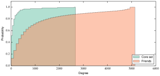
Figure 1: CDF of the degree distribution of users who liked a post by Kiva on Facebook and that of their friends.

An adaptive approach. An alternative approach to spending the entire budget on the core set is an adaptive two-stage approach. In the first stage, one can spend a fraction of the budget on the core users so that they invite their friends to participate in the campaign, then in the second stage spend the rest of the budget on the influential friends who hopefully have arrived. The idea behind this approach is to leverage a structural phenomenon in social networks known as the friendship paradox [9]. Intuitively, the friendship paradox says that individuals are not likely to have many friends, but they likely have a friend that does (“your friends have more friends than you”). In Figure 1 we give an example of such an effect by plotting a CDF of the degree distribution of a core set of users who responded to a post on Facebook and the degree distribution of their friends. Remarkably, there are also formal guarantees of such effects. Recent work shows that for any network that has a power law degree distribution and a small fraction of random edges, there is an asymptotic gap between the average degree of small samples of nodes and that of their neighbors, with constant probability [17]. The implication is that when considering the core users (e.g. those who visit the online store) as random samples from a social network, any algorithm which can use their neighbors as influencers will have dramatic improvement over the direct application of influence maximization.

Warmup. Suppose we are given a network, a random set of core users $X$ and a budget $k$, and the goal is to select a subset of nodes in $X$ of size $t\leq k$ which has the most influential set of neighbors of size $k-t$. For simplicity, assume for now that the influence of a set is simply its average degree. If we take the $k/2$ highest degree neighbors of $X$, then surely there is a set $S$ of size at most $k/2$ in $X$ connected to this set, and selecting $S$ would be a two-approximation to this problem. In comparison, the standard approach of influence maximization is to select the $k$ highest degree nodes in $X$. Thus, standard influence maximization would have $k$ of the most influential nodes in $X$ while the approximation algorithm we propose has $k/2$ of the most influential nodes from its set of neighbors. How much better or worse is it to use this approach over the standard one? If the network has a power-law degree distribution with a small fraction of random edges, and influence is measured in terms of sum of degrees of a set, then the results of [17] discussed above imply that the two-stage approach which allows seeding neighbors can do asymptotically (in the size of the network) better. Thus, at least intuitively, it looks as if two-stage approaches may be worth investigating.

In this paper, our goal is to study the potential benefits of adaptive approaches for influence maximization. We are largely motivated by the following question.

Can adaptive optimization lead to significant improvements in influence maximization?

To study this question we use the adaptive seeding model recently formalized in [26]. The main distinctions from the caricature model in the warmup problem above is that in adaptive seeding the core set $X$ can be arbitrary (it does not have to be random), and every neighbor of $X$ is assumed to arrive with some independent probability. These probabilities are used to model the uncertainty we have in that the neighbors would be interested in promoting the product, as they are not in the core set. The goal in adaptive seeding is to select a subset of nodes in $X$ such that, in expectation over all possible arrivals of its neighbors, one can select a maximally influential set of neighbors with the remaining budget. It is worth noting that using $X$ to be the entire set of nodes in the network we get the Kempe-Kleinberg-Tardos model [13], and thus adaptive seeding can be seen as a generalization of this model.

Scalability. One of the challenges in adaptive seeding is scalability. This is largely due to the stochastic nature of the problem derived from uncertainty about arrival of neighbors. The main result in [26] is a constant factor approximation algorithm for well-studied influence models such as independent cascade and linear threshold which is, at large, a theoretical triumph. These algorithms rely on various forms of sampling, which lead to a significant blowup in the input size. While such techniques provide strong theoretical guarantees, for social network data sets which are often either large or massive, such approaches are inapplicable. The main technical challenge we address in this work is how to design scalable adaptive optimization techniques for influence maximization which do not require sampling.

Beyond random users. The motivation for the adaptive approach hinges on the friendship paradox, but what if the core set is not a random sample? The results in [17] hold when the core set of users is random but since users who follow a particular topic are not a random sample of the network, we must somehow evaluate adaptive seeding on representative data sets. The experimental challenge is to estimate the prominence of high degree neighbors in settings that are typical of viral marketing campaigns. Figure 1 is a foreshadowing of the experimental methods we used to show that an effect similar to the friendship paradox exists in such cases as well.

Main results. Our main results in this paper show that adaptive seeding is a scalable approach which can dramatically improve upon standard approaches of influence maximization. We present a general method that enables designing adaptive seeding algorithms in a manner that avoids sampling, and thus makes adaptive seeding scalable to large size graphs. We use this approach as a basis for designing two algorithms, both achieving an approximation ratio of $(1-1/e)$ for the adaptive problem. The first algorithm is implemented through a linear program, which proves to be extremely efficient over instances where there is a large budget. The second approach is a combinatorial algorithm with the same approximation guarantee which can be easily parallelized, has good theoretical guarantees on its running time and does well on instances with smaller budgets. The guarantees of our algorithms hold for linear models of influence, i.e. models for which the influence of a set can be expressed as the sum of the influence of its members. While this class does not include models such as the independent cascade and the linear threshold model, it includes the well-studied voter model [12, 8] and measures such as node degree, click-through-rate or retweet measures of users which serve as natural proxies of influence in many settings [29]. In comparison to submodular influence functions, the relative simplicity of linear models allows making substantial progress on this challenging problem.

We then use these algorithms to conduct a series of experiments to show the potential of adaptive approaches for influence maximization both on synthetic and real social networks. The main component of the experiments involved collecting publicly available data from Facebook on users who expressed interest (“liked”) a certain post from a topic they follow and data on their friends. The premise here is that such users mimic potential participants in a viral marketing campaign. The results on these data sets suggest that adaptive seeding can have dramatic improvements over standard influence maximization methods.

Paper organization. We begin by formally describing the model and the assumptions we make in the following section. In Section 3 we describe the reduction of the adaptive seeding problem to a non-adaptive relaxation. In Section 4 we describe our non-adaptive algorithms for adaptive seeding. In Section 5 we describe our experiments, and conclude with a brief discussion on related work.

2 Model

Given a graph $G=(V,E)$, for a node $v\in V$ we denote by $\mathcal{N}(v)$ the neighborhood of $v$. By extension, for any subset of nodes $S\subseteq V$, $\mathcal{N}(S)\equiv\bigcup_{v\in S}\mathcal{N}(v)$ will denote the neighborhood of $S$. The notion of influence in the graph is captured by a function $f:2^{|V|}\rightarrow\mathbf{R}_{+}$ mapping a subset of nodes to a non-negative influence value.

The adaptive seeding model. The input of the adaptive seeding problem is a core set of nodes $X\subseteq V$ and for any node $u\in\mathcal{N}(X)$ a probability $p_{u}$ that $u$ realizes if one of its neighbor in $X$ is seeded. We will write $m=|X|$ and $n=|\mathcal{N}(X)|$ the parameters controlling the input size. The seeding process is the following:

1. Seeding: the seeder selects a subset of nodes $S\subseteq X$ in the core set.

2. Realization of the neighbors: every node $u\in\mathcal{N}(S)$ realizes independently with probability $p_{u}$. We denote by $R\subseteq\mathcal{N}(S)$ the subset of nodes that is realized during this stage.

3. Influence maximization: the seeder selects the set of nodes $T\subseteq R$ that maximizes the influence function $f$.

There is a budget constraint $k$ on the total number of nodes that can be selected: $S$ and $T$ must satisfy $|S|+|T|\leq k$. The seeder chooses the set $S$ before observing the realization $R$ and thus wishes to select optimally in expectation over all such possible realizations. Formally, the objective can be stated as:

$$\begin{split}&\max_{S\subseteq X}\sum_{R\subseteq\mathcal{N}(S)}p_{R}\max_{\begin{subarray}{c}T\subseteq R\\ |T|\leq k-|S|\end{subarray}}f(T)\\ &\text{s.t. }|S|\leq k\end{split}$$ (1)

where $p_{R}$ is the probability that the set $R$ realizes, $p_{R}\equiv\prod_{u\in R}p_{u}\prod_{u\in\mathcal{N}(S)\setminus R}(1-p_{u})$.

It is important to note that the process through which nodes arrive in the second stage is not an influence process. The nodes in the second stage arrive if they are willing to spread information in exchange for a unit of the budget. Only when they have arrived does the influence process occur. This process is encoded in the influence function and occurs after the influence maximization stage without incentivizing nodes along the propagation path. In general, the idea of a two-stage (or in general, multi-stage) approach is to use the nodes who arrive in the first stage to recruit influential users who can be incentivized to spread information. In standard influence maximization, the nodes who are not in the core set do not receive incentives to propagate information, and cascades tend to die off quickly [28, 3, 10, 6].

Influence functions. In this paper we focus on linear (or additive) influence models: in these models the value of a subset of nodes can be expressed as a weighted sum of their individual influence. One important example of such models is the voter model [25] used to represent the spread of opinions in a social network: at each time step, a node adopts an opinion with a probability equal to the fraction of its neighbors sharing this opinion at the previous time step. Formally, this can be written as a discrete-time Markov chain over opinion configurations of the network. In this model influence maximization amounts to “converting” the optimal subset of nodes to a given opinion at the initial time so as to maximize the number of converts after a given period of time. Remarkably, a simple analysis shows that under this model, the influence function $f$ is additive:

$$\forall S\subseteq V,\;f(S)=\sum_{u\in S}w_{u}$$ (2)

where $w_{u},u\in V$ are weights which can be easily computed from the powers of the transition matrix of the Markov chain. This observation led to the development of fast algorithms for influence maximization under the voter model [8].

NP-Hardness. In contrast to standard influence maximization, adaptive seeding is already NP-Hard even for the simplest influence functions such as $f(S)=|S|$ and when all probabilities are one. We discuss this in Appendix B.

3 Non-adaptive Optimization

The challenging aspect of the adaptive seeding problem expressed in Equation 1 is its adaptivity: a seed set must be selected during the first stage such that in expectation a high influence value can be reached when adaptively selecting nodes on the second stage. A standard approach in stochastic optimization for overcoming this challenge is to use sampling to estimate the expectation of the influence value reachable on the second stage. However, as will be discussed in Section 5, this approach quickly becomes infeasible even with modest size graphs.

In this section we develop an approach which avoids sampling and allows designing adaptive seeding algorithms that can be applied to large graphs. We show that for additive influence functions one can optimize a relaxation of the problem which we refer to as the non-adaptive version of the problem. After defining the non-adaptive version, we show in sections 3.1 that the optimal solution for the non-adaptive version is an upper bound on the optimal solution of the adaptive seeding problem. We then argue in Section 3.2 that any solution to the non-adaptive version of the problem can be converted to an adaptive solution, losing an arbitrarily small factor in the approximation ratio. Together, this implies that one can design algorithms for the non-adaptive problem instead, as we do in Section 4.

Non-adaptive policies. We say that a policy is non-adaptive if it selects a set of nodes $S\subseteq X$ to be seeded in the first stage and a vector of probabilities $\mathbf{q}\in[0,1]^{n}$, such that each neighbor $u$ of $S$ which realizes is included in the solution independently with probability $q_{u}$. The constraint will now be that the budget is only respected in expectation, i.e. $|S|+\textbf{p}^{T}\textbf{q}\leq k$. Formally the optimization problem for non-adaptive policies can be written as:

$$\begin{split}\max_{\begin{subarray}{c}S\subseteq X\\ \textbf{q}\in[0,1]^{n}\end{subarray}}&\;\sum_{R\subseteq\mathcal{N}(X)}\Big{(}\prod_{u\in R}p_{u}q_{u}\prod_{u\in\mathcal{N}(X)\setminus R}(1-p_{u}q_{u})\Big{)}f(R)\\ \text{s.t. }&\;|S|+\textbf{p}^{T}\textbf{q}\leq k,\;q_{u}\leq\mathbf{1}\{u\in\mathcal{N}(S)\}\end{split}$$ (3)

where we denote by $\mathbf{1}\{E\}$ the indicator variable of the event $E$. Note that because of the condition $q_{u}\leq\mathbf{1}\{u\in\mathcal{N}(S)\}$, the summand associated with $R$ in (3) vanishes whenever $R$ contains $u\in\mathcal{N}(X)\setminus\mathcal{N}(S)$. Hence, the summation is restricted to $R\subseteq\mathcal{N}(S)$ as in (1).

3.1 Adaptivity Gap

We will now justify the use of non-adaptive strategies by showing that the optimal solution for this form of non-adaptive strategies yields a higher value than adaptive ones. For brevity, given a probability vector $\pi\in[0,1]^{m}$ we write:

$$F(\pi)\equiv\sum_{R\subseteq\mathcal{N}(X)}\left(\prod_{u\in R}\pi_{u}\prod_{u\in\mathcal{N}(X)\setminus R}(1-\pi_{u})\right)f(R)$$ (4)

as well as $\textbf{p}\otimes\textbf{q}$ to denote the component-wise multiplication between vectors p and q. Finally, we write $\mathcal{F}_{A}\equiv\{S\subseteq X:|S|\leq k\}$, and $\mathcal{F}_{NA}\equiv\{(S,\textbf{q}),|S|+\textbf{p}^{T}\textbf{q}\leq k,q_{u}\leq\mathbf{1}_{\{u\in\mathcal{N}(S)\}}\}$ to denote the feasible regions of the adaptive and non-adaptive problems, respectively.

Proposition 1

For additive functions given by (2), the value of the optimal adaptive policy is upper bounded by the optimal non-adaptive policy:

$$\begin{aligned} &\max_{S\subseteq X}\sum_{R\subseteq\mathcal{N}(S)}p_{R}\max_{\begin{subarray}{c}T\subseteq R\\ |T|\leq k-|S|\end{subarray}}f(T)\\ &\text{s.t. }S\in\mathcal{F}_{A}\end{aligned}\leq\begin{aligned} &\max_{\begin{subarray}{c}S\subseteq X\\ \textbf{q}\in[0,1]^{n}\end{subarray}}F(\mathbf{p}\otimes\mathbf{q})\\ &\text{s.t. }(S,\textbf{q})\in\mathcal{F}_{NA}\end{aligned}$$

The proof of this proposition can be found in Appendix A and relies on the following fact: the optimal adaptive policy can be written as a feasible non-adaptive policy, hence it provides a lower bound on the value of the optimal non-adaptive policy.

3.2 From Non-Adaptive to Adaptive Solutions

From the above proposition we now know that optimal non-adaptive solutions have higher values than adaptive solutions. Given a non-adaptive solution $(S,\mathbf{q})$, a possible scheme would be to use $S$ as an adaptive solution. But since $(S,\mathbf{q})$ is a solution to the non-adaptive problem, Proposition 1 does not provide any guarantee on how well $S$ performs as an adaptive solution.

However, we show that from a non-adaptive solution $(S,\mathbf{q})$, we can obtain a lower bound on the adaptive value of $S$, that is, the expected influence attainable in expectation over all possible arrivals of neighbors of $S$. Starting from $S$, in every realization of neighbors $R$, sample every node $u\in R\cap\mathcal{N}(S)$ with probability $q_{u}$, to obtain a random set of nodes $I_{R}\subseteq R\cap S$. $(S,\mathbf{q})$ being a non-adaptive solution, it could be that selecting $I_{R}$ exceeds our budget. Indeed, the only guarantee that we have is that $|S|+\mathbb{E}\big{[}|I_{R}|\big{]}\leq k$. As a consequence, an adaptive solution starting from $S$ might not be able to select $I_{R}$ on the second stage.

Fortunately, the probability of exceeding the budget is small enough and with high probability $I_{R}$ will be feasible. This is exploited in [27] to design a randomized rounding method with approximation guarantees. These rounding methods are called contention resolution schemes. Theorem 1.3 of this paper gives us a contention resolution scheme which will compute from $\mathbf{q}$ and for any realization $R$ a feasible set $\tilde{I}_{R}$, such that:

$$\mathbb{E}_{R}\big{[}f(\tilde{I}_{R})\big{]}\geq(1-\varepsilon)F(\mathbf{q})$$ (5)

What this means is that starting from a non-adaptive solution $(S,\mathbf{q})$, there is a way to construct a random feasible subset on the second stage such that in expectation, this set attains almost the same influence value as the non-adaptive solution. Since the adaptive solution starting from $S$ will select optimally from the realizations $R\subseteq\mathcal{N}(S)$, $\mathbb{E}_{R}[f(\tilde{I}_{R})]$ provides a lower bound on the adaptive value of $S$ that we denote by $A(S)$.

More precisely, denoting by $\text{OPT}_{A}$ the optimal value of the adaptive problem (1), we have the following proposition whose proof can be found in Appendix A.

Proposition 2

Let $(S,\textbf{q})$ be an $\alpha$-approximate solution to the non-adaptive problem (3), then $\mathrm{A}(S)\geq\alpha\mathrm{OPT}_{A}$.

4 Algorithms

Section 3 shows that the adaptive seeding problem reduces to the non-adaptive problem. We will now discuss two approaches to construct approximate non-adaptive solutions. The first is an LP-based approach, and the second is a combinatorial algorithm. Both approaches have the same $(1-1/e)$ approximation ratio, which is then translated to a $(1-1/e)$ approximation ratio for the adaptive seeding problem (1) via Proposition 2. As we will show in Section 5, both algorithms have their advantages and disadvantages in terms of scalability.

4.1 An LP-Based Approach

Note that due to linearity of expectation, for a linear function $f$ of the form given by (2) we have:

$$\begin{split}F(\textbf{p})&=\mathbb{E}_{R}\big{[}f(R)\big{]}=\mathbb{E}_{R}\Bigg{[}\sum_{u\in\mathcal{N}(X)}w_{u}\mathbf{1}_{\{u\in R\}}\Bigg{]}\\ &=\sum_{u\in\mathcal{N}(X)}w_{u}\mathbb{P}[u\in R]=\sum_{u\in\mathcal{N}(X)}p_{u}w_{u}\end{split}$$ (6)

Thus, the non-adaptive optimization problem (3) can be written as:

$$\begin{split}\max_{\begin{subarray}{c}S\subseteq X\\ \mathbf{q}\in[0,1]^{n}\end{subarray}}&\sum_{u\in\mathcal{N}(X)}p_{u}q_{u}w_{u}\\ \text{s.t. }&|S|+\textbf{p}^{T}\textbf{q}\leq k,\;q_{u}\leq\mathbf{1}\{u\in\mathcal{N}(S)\}\end{split}$$

The choice of the set $S$ can be relaxed by introducing a variable $\lambda_{v}\in[0,1]$ for each $v\in X$. We obtain the following LP for the adaptive seeding problem:

$$\begin{split}\max_{\begin{subarray}{c}\mathbf{q}\in[0,1]^{n}\\ \boldsymbol{\lambda}\in[0,1]^{m}\end{subarray}}&\;\sum_{u\in\mathcal{N}(X)}p_{u}q_{u}w_{u}\\ \text{s.t. }&\sum_{v\in X}\lambda_{v}+\textbf{p}^{T}\textbf{q}\leq k,\;q_{u}\leq\sum_{v\in\mathcal{N}(u)}\lambda_{v}\end{split}$$ (7)

An optimal solution to the above problem can be found in polynomial time using standard LP-solvers. The solution returned by the LP is fractional, and requires a rounding procedure to return a feasible solution to our problem, where $S$ is integral. To round the solution we use the pipage rounding method [2]. We defer the details to Appendix B.1.

Lemma 1

For AdaptiveSeeding-LP defined in (7), any fractional solution $(\boldsymbol{\lambda},\mathbf{q})\in[0,1]^{m}\times[0,1]^{n}$ can be rounded to an integral solution $\bar{\boldsymbol{\lambda}}\in\{0,1\}^{m}$ s.t. $(1-1/e)F(\mathbf{p}\circ\mathbf{q})\leq A(\bar{\lambda})$ in $O(m+n)$ steps.

4.2 A Combinatorial Algorithm

In this section, we introduce a combinatorial algorithm with an identical approximation guarantee to the LP-based approach. However, its running time, stated in Proposition 5 can be better than the one given by LP solvers depending on the relative sizes of the budget and the number of nodes in the graph. Furthermore, as we discuss at the end of this section, this algorithm is amenable to parallelization.

The main idea is to reduce the problem to a monotone submodular maximization problem and apply a variant of the celebrated greedy algorithm [23]. In contrast to standard influence maximization, the submodularity of the non-adaptive seeding problem is not simply a consequence of properties of the influence function; it also strongly relies on the combinatorial structure of the two-stage optimization.

Intuitively, we can think of our problem as trying to find a set $S$ in the first stage, for which the nodes that can be seeded on the second stage have the largest possible value. To formalize this, for a budget $b\in\mathbf{R}^{+}$ used in the second stage and a set of neighbors $T\subseteq\mathcal{N}(X)$, we will use $\mathcal{O}(T,b)$ to denote the solution to:

$$\begin{split}\mathcal{O}(T,b)\equiv\max_{\textbf{q}\in[0,1]^{n}}&\sum_{u\in\mathcal{N}(X)\cap T}p_{u}q_{u}w_{u}\\ \text{s.t. }&\mathbf{p}^{T}\mathbf{q}\leq b\end{split}$$ (8)

The optimization problem (3) for non-adaptive policies can now be written as:

$$\max_{S\subseteq X}\;\mathcal{O}\big{(}\mathcal{N}(S),k-|S|\big{)}\quad\text{s.t. }|S|\leq k$$ (9)

We start by proving in Proposition 3 that for fixed $t$, $\mathcal{O}(\mathcal{N}(\cdot),t)$ is submodular. This proposition relies on lemmas 2 and 3 about the properties of $\mathcal{O}(T,b)$.

Lemma 2

Let $T\subseteq\mathcal{N}(X)$ and $x\in\mathcal{N}(X)$, then $\mathcal{O}(T\cup\{x\},b)-\mathcal{O}(T,b)$ is non-decreasing in $b$.

The proof of this lemma can be found in Appendix B.2. The main idea consists in writing:

$$\mathcal{O}(T\cup\{x\},c)-\mathcal{O}(T\cup\{x\},b)=\int_{b}^{c}\partial_{+}\mathcal{O}_{T\cup\{x\}}(t)dt$$

where $\partial_{+}\mathcal{O}_{T}$ denotes the right derivative of $\mathcal{O}(T,\cdot)$. For a fixed $T$ and $b$, $\mathcal{O}(T,b)$ defines a fractional Knapsack problem over the set $T$. Knowing the form of the optimal fractional solution, we can verify that $\partial_{+}\mathcal{O}_{T\cup\{x\}}\geq\partial_{+}\mathcal{O}_{T}$ and obtain:

$$\mathcal{O}(T\cup\{x\},c)-\mathcal{O}(T\cup\{x\},b)\geq\mathcal{O}(T,c)-\mathcal{O}(T,b)$$

Lemma 3

For any $b\in\mathbf{R}^{+}$, $\mathcal{O}(T,b)$ is submodular in $T$, $T\subseteq\mathcal{N}(X)$.

The proof of this lemma is more technical. For $T\subseteq\mathcal{N}(X)$ and $x,y\in\mathcal{N}(X)\setminus T$, we need to show that:

$$\mathcal{O}(T\cup\{x\},b)-\mathcal{O}(T,b)\geq\mathcal{O}(T\cup\{y,x\},b)-\mathcal{O}(T\cup\{y\},b)$$

This can be done by partitioning the set $T$ into “high value items” (those with weight greater than $w_{x}$) and “low value items” and carefully applying Lemma 2 to the associated subproblems. The proof is in Appendix B.2.

Finally, Lemma 3 can be used to show Proposition 3 whose proof can be found in Appendix B.2.

Proposition 3

Let $b\in\mathbf{R}^{+}$, then $\mathcal{O}(\mathcal{N}(S),b)$ is monotone and submodular in $S$, $S\subseteq X$.

We can now use Proposition 3 to reduce (9) to a monotone submodular maximization problem. First, we note that (9) can be rewritten:

$$\max_{\begin{subarray}{c}S\subseteq X\\ t\in\mathbb{N}\end{subarray}}\;\mathcal{O}\big{(}\mathcal{N}(S),t\big{)}\quad\text{s.t. }|S|+t\leq k$$ (10)

Intuitively, we fix $t$ arbitrarily so that the maximization above becomes a submodular maximization problem with fixed budget $t$. We then optimize over the value of $t$. Combining this observation with the greedy algorithm for monotone submodular maximization [23], we obtain Algorithm 1, whose performance guarantee is summarized in Proposition 4.

Algorithm 1 Combinatorial algorithm

1:  $S\leftarrow\emptyset$

2:  for $t=1$ to $k-1$ do

3:        $S_{t}\leftarrow\emptyset$

4:        for $i=1$ to $k-t$ do

5:              $x^{*}\leftarrow\operatorname*{argmax}_{x\in X\setminus S_{t}}\mathcal{O}(\mathcal{N}(S_{t}\cup\{x\}),t)-\mathcal{O}(\mathcal{N}(S_{t}),t)$

6:              $S_{t}\leftarrow S_{t}\cup\{x^{*}\}$

7:        end for

8:        if $\mathcal{O}(\mathcal{N}(S_{t}),t)>\mathcal{O}(\mathcal{N}(S),k-|S|)$ then

9:              $S\leftarrow S_{t}$

10:        end if

11:  end for

12:  return  $S$

Proposition 4

Let $S$ be the set computed by Algorithm 1 and let us denote by $\mathrm{A}(S)$ the value of the adaptive policy selecting $S$ on the first stage. Then $\mathrm{A}(S)\geq(1-1/e)\mathrm{OPT}_{A}$.

Parallelization. The algorithm described above considers all possible ways to split the seeding budget between the first and the second stage. For each possible split $\{(t,k-t)\}_{t=1\ldots,k-1}$, the algorithm computes an approximation to the optimal non adaptive solution that uses $k-t$ nodes in the first stage and $t$ nodes in the second stage, and returns the solution for the split with the highest value (breaking ties arbitrarily). This process can be trivially parallelized across $k-1$ machines, each performing a computation of a single split. With slightly more effort, for any $\epsilon>0$ one can parallelize over $\log_{1+\epsilon}n$ machines at the cost of losing a factor of $\epsilon$ in the approximation guarantee (see Appendix B.3 for details).

Implementation in MapReduce. While the previous paragraph describes how to parallelize the outer for loop of Algorithm 1, we note that its inner loop can also be parallelized in the MapReduce framework. Indeed, it corresponds to the greedy algorithm applied to the function $\mathcal{O}\left(\mathcal{N}(\cdot),t\right)$. The Sample&Prune approach successfully applied in [16] to obtain MapReduce algorithms for various submodular maximizations can also be applied to Algorithm 1 to cast it in the MapReduce framework. The details of the algorithm can be found in Appendix B.4.

Algorithmic speedups. To implement Algorithm 1 efficiently, the computation of the $\operatorname*{argmax}$ on line 5 must be dealt with carefully. $\mathcal{O}(\mathcal{N}(S_{t}\cup\{x\}),t)$ is the optimal solution to the fractional Knapsack problem (8) with budget $t$ and can be computed in time $\min(\frac{t}{p_{\text{min}}},n)$ by iterating over the list of nodes in $\mathcal{N}(S_{t}\cup\{x\})$ in decreasing order of the degrees. This decreasing order of $\mathcal{N}(S_{t})$ can be maintained throughout the greedy construction of $S_{t}$ by:

• ordering the list of neighbors of nodes in $X$ by decreasing order of the degrees when initially constructing the graph. This is responsible for a $O(n\log n)$ pre-processing time.

• when adding node $x$ to $S_{t}$, observe that $\mathcal{N}(S_{t}\cup\{x\})=\mathcal{N}(S_{t})\cup\mathcal{N}(\{x\})$. Hence, if $\mathcal{N}(S_{t})$ and $\mathcal{N}(\{x\})$ are sorted lists, then $\mathcal{O}(\mathcal{N}(S_{t}\cup\{x\}),t)$ can be computed in a single iteration of length $\min(\frac{t}{p_{\text{min}}},n)$ where the two sorted lists are merged on the fly.

As a consequence, the running time of line 5 is bounded from above by $m\min(\frac{t}{p_{\text{min}}},n)$. The two nested for loops are responsible for the additional $k^{2}$ factor. The running time of Algorithm 1 is summarized in Proposition 5.

Proposition 5

Let $p_{\text{min}}=\min\{p_{u},u\in\mathcal{N}(X)\}$, then Algorithm 1 runs in time ${O\big{(}n\log n+k^{2}m\min(\frac{k}{p_{\text{min}}},n)\big{)}}$.

5 Experiments

In this section we validate the adaptive seeding approach through experimentation. Specifically, we show that our algorithms for adaptive seeding obtain significant improvement over standard influence maximization, that these improvements are robust to changes in environment variables, and that our approach is efficient in terms of running-time and scalable to large social networks.

5.1 Experimental setup

We tested our algorithms on three types of datasets. Each of them allows us to experiment on a different aspect of the adaptive seeding problem. The Facebook Pages dataset that we collected ourselves has a central place in our experiments since it is the one which is closet to actual applications of adaptive seeding.

Synthetic networks. Using standard models of social networks we generated large-scale graphs to model the social network. To emulate the process of users following a topic (the core set $X$) we sampled subsets of nodes at random, and applied our algorithms on the sample and their neighbors. The main advantage of these data sets is that they allow us to generate graphs of arbitrary sizes and experiment with various parameters that govern the structure of the graph. The disadvantages are that users who follow a topic are not necessarily random samples, and that social networks often have structural properties that are not captured in generative models.

Real networks. We used publicly available data sets of real social networks available at [20]. As for synthetic networks, we used a random sample of nodes to emulate users who follow a topic, which is the main disadvantage of this approach. The advantage however, is that such datasets contain an entire network which allows testing different propagation parameters.

Facebook Pages. We collected data from several Facebook Pages, each associated with a commercial entity that uses the Facebook page to communicate with its followers. For each page, we selected a post and then collected data about the users who expressed interest (“liked”) the post and their friends. The advantage of this data set is that it is highly representative of the scenario we study here. Campaigns run on a social network will primarily target users who have already expressed interests in the topic being promoted. The main disadvantage of this method is that such data is extremely difficult to collect due to the crawling restrictions that Facebook applies and gives us only the 2-hop neighborhood around a post. This makes it difficult to experiment with different propagation parameters. Fortunately, as we soon discuss, we were able to circumvent some of the crawling restrictions and collect large networks, and the properties of the voter influence model are such that these datasets suffice to accurately account for influence propagation in the graph.

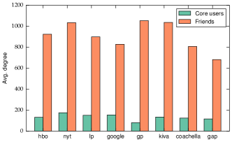
Figure 2: Comparison of the average degree of the core set users and the average degree of their friends.

Data collection. We selected Facebook Pages in different verticals (topics). Each page is operated by an institution or an entity whose associated Facebook Page is regularly used for promotional posts related to this topic. On each of these pages, we selected a recent post (posted no later than January 2014) with approximately 1,000 likes. The set of users who liked those posts constitute our core set. We then crawled the social network of these sets: for each user, we collected her list of friends, and the degrees (number of friends) of these friends.

Data description. Among the several verticals we collected, we select eight of them for which we will report our results. We obtained similar results for the other ones. Table 1 summarizes statistics about the selected verticals. We note that depending on the privacy settings of the core set users, it was not always possible to access their list of friends. We decided to remove these users since their ability to spread information could not be readily determined. This effect, combined with various errors encountered during the data collection, accounts for an approximate 15% reduction between the users who liked a post and the number of users in the datasets we used. Following our discussion in the introduction, we observe that on average, the degrees of core set users is much lower than the degrees of their friends. This is highlighted on Figure 2 and justifies our approach.

Vertical	Page	$m$	$n$
Charity	Kiva	978	131334
Travel	Lonely Planet	753	113250
Fashion	GAP	996	115524
Events	Coachella	826	102291
Politics	Green Party	1044	83490
Technology	Google Nexus	895	137995
News	The New York Times	894	156222
Entertainment	HBO	828	108699

Table 1: Dataset statistics. $m$: number of users in the core set, $n$: number of friends of core set users.

5.2 Performance of Adaptive Seeding

For a given problem instance with a budget of $k$ we applied the adaptive seeding algorithm (the combinatorial version). Recall from Section 2 that performance is defined as the expected influence that the seeder can obtain by optimally selecting users on the second stage, where influence is defined as the sum of the degrees of the selected users. We tested our algorithm against the following benchmarks:

• Random Node (RN): we randomly select $k$ users from the core set. This is a typical benchmark in comparing influence maximization algorithms [13].

• Influence Maximization (IM): we apply the optimal influence maximization algorithm on the core set. This is the naive application of influence maximization. For the voter model, when the propagation time is polynomially large in the network size, the optimal solution is to simply take the $k$ highest degree nodes [8]. We study the case of bounded time horizons in Section 5.5.

• Random Friend (RF): we implement a naive two-stage approach: randomly select $k/2$ nodes from the core set, and for each node select a random neighbor (hence spending the budget of $k$ rewards overall). This method was recently shown to outperform standard influence maximization when the core set is random [17].

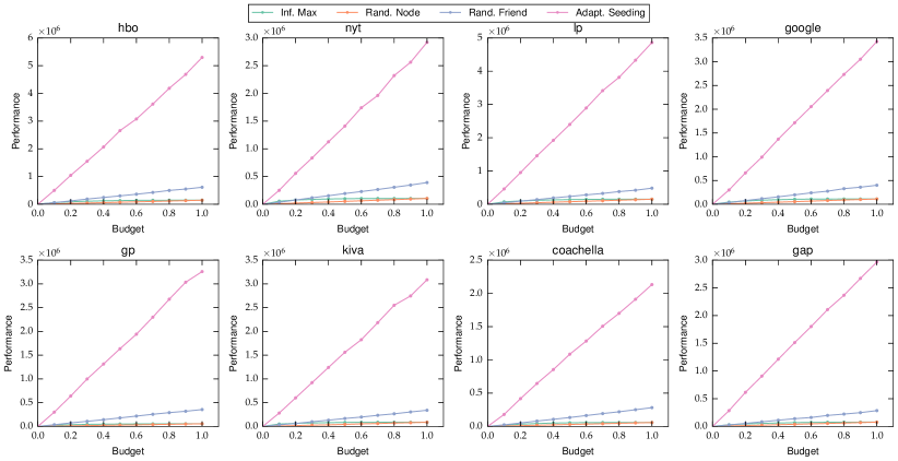
Figure 3: Performance of adaptive seeding compared to other influence maximization approaches. The horizontal axis represents the budget used as a fraction of the size of the core set. The vertical axis is the expected influence reachable by optimally selecting nodes on the second stage.

5.3 Performance on Facebook Pages

Figure 3 compares the performance of adaptive seeding, our own approach, to the afore-mentioned approaches for all the verticals we collected. In this first experiment we made simplifying assumptions about the parameters of the model. The first assumption is that all probabilities in the adaptive seeding model are equal to one. This implicitly assumes that every friend of a user who followed a certain topic is interested in promoting the topic given a reward. Although this is a strong assumption that we will revisit, we note that the probabilities can be controlled to some extent by the social networking service on which the campaign is being run by showing prominently the campaign material (sponsored links, fund-raising banners, etc.). The second assumption is that the measure of influence is the sum of the degrees of the selected set. This measure is an appealing proxy as it is known that in the voter model, after polynomially many time steps, the influence of each node is proportional to its degree with high probability [8]. Since the influence process cannot be controlled by the designer, the assumption is often that the influence process runs until it stabilizes (in linear thresholds and independent cascades for example, the process terminates after a linear number of steps [13]). We perform a set of experiments for different time horizons in Section 5.5.

It is striking to see how well adaptive seeding does in comparison to other methods. Even when using a small budget (0.1 fraction of the core set, which in these cases is about 100 nodes), adaptive seeding improves influence by a factor of at least 10, across all verticals. To confirm this, we plot the relative improvements of adaptive seeding over IM in aggregate over the different pages. The results are shown in Figure 4. This dramatic improvement is largely due to the friendship paradox phenomenon that adaptive seeding leverages. Returning to Figure 3, it is also interesting to note that the RF heuristic significantly outperforms the standard IM benchmark. Using the same budget, the degree gain induced by moving from the core set to its neighborhood is such that selecting at random among the core set users’ friends already does better than the best heuristic restricted only on the core set. Using adaptive seeding to optimize the choice of core set users based on their friends’ degrees then results in an order of magnitude increase over RF, consistently for all the pages.

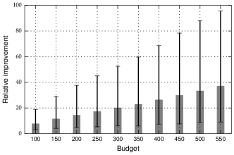
Figure 4: Ratio of the performance of adaptive seeding to IM. Bars represents the mean improvement across all verticals, and the “error bar” represents the range of improvement across verticals.

5.4 The Effect of the Probabilistic Model

The results presented in Section 5.2 were computed assuming the probabilities in the adaptive seeding model are one. We now describe several experiments we performed with the Facebook Pages data set that test the advantages of adaptive seeding under different probability models.

Impact of the Bernouilli parameter. Figure 5(a) shows the impact of the probability of nodes realizing in the second stage. We computed the performance of adaptive seeding when each friend of a seeded user in the core set joins during the second stage independently with probability $p$, using different values of $p$. We call $p$ the Bernouilli parameter, since the event that a given user joins on the second stage of adaptive seeding is governed by a Bernouilli variable of parameter $p$. We see that even with $p=0.01$, adaptive seeding still outperforms IM. As $p$ increases, the performance of adaptive seeding quickly increases and reaches $80\%$ of the values of Figure 3 at $p=0.5$.

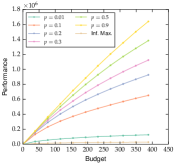
(a)

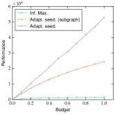
(b)

Figure 5: (a) Performance of adaptive seeding for various propagation probabilities. (b) Performance of adaptive seeding when restricted to the subgraph of users who liked HBO (red line).

Coarse estimation of probabilities. In practice, the probability a user may be interested in promoting a campaign her friend is promoting may vary. However, for those who have already expressed interest in the promoted content, we can expect this probability to be close to one. We therefore conducted the following experiment. We chose a page (HBO) and trimmed the social graph we collected by only keeping on the second stage users who indicated this page (HBO) in their list of interests. This is a coarse estimation of the probabilities as it assumes that if a friend follows HBO she will be willing to promote with probability 1 (given a reward), and otherwise the probability of her promoting anything for HBO is 0. Figure 5(b) shows that even on this very restricted set of users, adaptive seeding still outperforms IM and reaches approximately $50\%$ of the unrestricted adaptive seeding.

Impact of the probability distribution. In order to test scenarios where users have a rich spectrum of probabilities of realizing on the second stage. We consider a setting where the Bernouilli parameter $p$ is drawn from a distribution. We considered four different distributions; for each distribution for fixed values of the budget and the parameter $p$, we tuned the parameters of the distribution so that its mean is exactly $p$. We then plotted the performance as a function of the budget and mean $p$.

For the Beta distribution, we fixed $\beta=5$ and tuned the $\alpha$ parameter to obtain a mean of $p$, thus obtaining a unimodal distribution. For the normal distribution, we chose a standard deviation of $0.01$ to obtain a distribution more concentrated around its mean than the Beta distribution. Finally, for the inverse degree distribution, we took the probability of a node joining on the second stage to be proportional to the inverse of its degree (scaled so that on average, nodes join with probability $p$). The results are shown in Figure 6(d).

We observe that the results are comparable to the one we obtained in the uniform case in Figure 5(a) except in the case of the inverse degree distribution for which the performance is roughly halved. Remember that the value of a user $v$ on the second stage of adaptive seeding is given by $p_{v}d_{v}$ where $d_{v}$ is its degree and $p_{v}$ is the its probability of realizing on the second stage. Choosing $p_{v}$ to be proportional to ${1}/{d_{v}}$ has the effect of normalizing the nodes on the second stage and is a strong perturbation of the original degree distribution of the nodes available on the second stage.

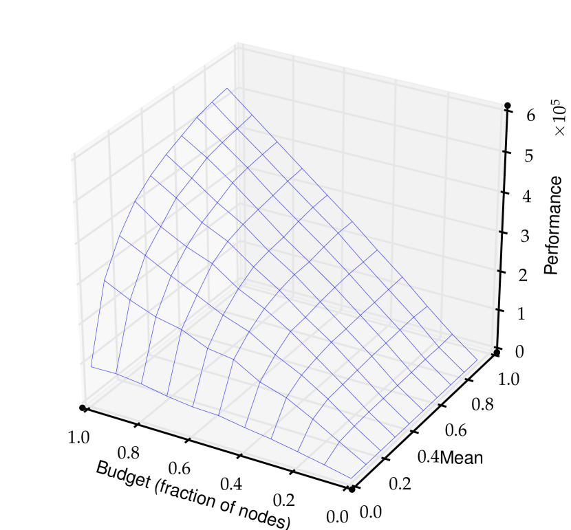
(a) Beta distribution

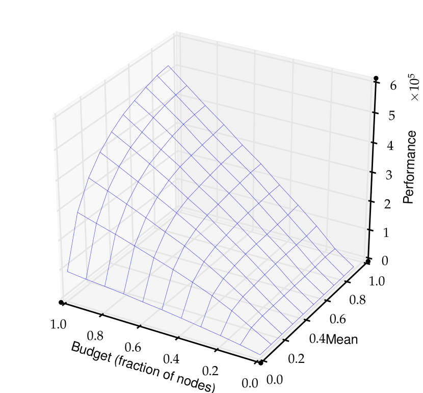
(b) Normal Distribution

(c) Power-law distribution

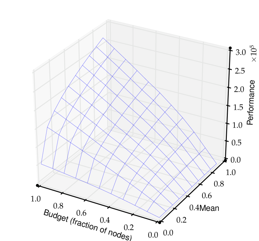
(d) Inverse degree

Figure 6: Performance of adaptive seeding as a function of the budget and the mean of the distribution from which the Bernouilli parameters are drawn. The details of the parameters for each distribution can be found in Section 5.4.

.

5.5 Impact of the Influence Model

The Facebook Pages data set we collected is limited in that we only have access to the 2-hop neighborhood around the seed users and we use the degree of the second stage users as a proxy for their influence. As proved in [8], in the voter model, the influence of nodes converges to their degree with high probability when the number of time steps become polynomially large in the network size.

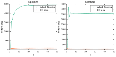
Figure 7: Performance of adaptive seeding compared to IM for the voter influence model with $t$ steps.

In order to analyze the expected number of nodes influenced according to the voter model that terminates after some fixed number of time steps, we use publicly available data sets from [20] where the entire network is at our disposal. As discussed above, we sample nodes uniformly at random to model the core set. We then run the voter model for $t$ time steps to compute the influence of the second stage users. Figure 7 shows the performance of adaptive seeding as a function of $t$ compared to the performance of the IM benchmark. In this experiment, the budget was set to half the size of the core set.

We see that the performance of adaptive seeding quickly converges (5 time steps for Slashdot, 15 time steps for Epinions). In practice, the voter model converges much faster than the theoretical guarantee of [8], which justifies using the degree of the second stage users as measure of influence as we did for the Facebook Pages data sets. Furthermore, we see that similarly to the Facebook data sets, adaptive seeding significantly outperforms IM.

5.6 Performance on Synthetic Networks

In order to analyze the impact of topological variations we generated synthetic graphs using standard network models. All the generated graphs have $100,000$ vertices, for each model, we tuned the generative parameters to obtain when possible a degree distribution (or graph density otherwise) similar to what we observed in the Facebook Pages data sets.

• Barabási-Albert: this well-known model is often used to model social graphs because its degree distribution is a power law. We took 10 initial vertices and added 10 vertices at each step, using the preferential attachment model, until we reached 100,000 vertices.

• Small-World: also known as the Watts-Strogatz model. This model was one of the first models proposed for social networks. Its diameter and clustering coefficient are more representative of a social network than what one would get with the Erdős–Rényi model. We started from a regular lattice of degree 200 and rewired each edge with probability 0.3.

• Kronecker: Kronecker graphs were more recently introduced in [18] as a scalable and easy-to-fit model for social networks. We started from a star graph with 4 vertices and computed Kronecker products until we reached 100,000 nodes.

• Configuration model: The configuration model allows us to construct a graph with a given degree distribution. We chose a page (GAP) and generated a graph with the same degree distribution using the configuration model.

The performance of adaptive seeding compared to our benchmarks can be found in Figure 8. We note that the improvement obtained by adaptive seeding is comparable to the one we had on real data except for the Small-World model. This is explained by the nature of the model: starting from a regular lattice, some edges are re-wired at random. This model has similar properties to a random graph where the friendship paradox does not hold [17]. Since adaptive seeding is designed to leverage the friendship paradox, such graphs are not amenable to this approach.

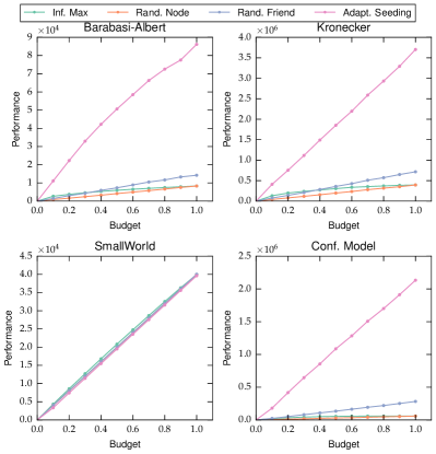
Figure 8: Performance of adaptive seeding on synthetic networks.

5.7 Scalability

To test the scalability of adaptive seeding we were guided by two central questions. First, we were interested to witness the benefit our non-sampling approach has over the standard SAA method. Secondly, we wanted to understand when one should prefer to use the LP-based approach from Section 4.1 over the combinatorial one from Section 4.2. The computations in this section were run on Intel Core i5 CPU 4x2.40Ghz. For each computation, we plot the time and number of CPU cycles it took.

Comparison with SAA. The objective function of the non-adaptive problem (3) is an expectation over exponentially many sets, all possible realizations of the neighbors in the second stage. Following the sampling-based approach introduced in [26], this expectation can be computed by averaging the values obtained in $O\left(n^{2}\right)$ independent sample realizations of the second stage users ($n$ is the number of neighbors of core set users). One important aspect of the algorithms introduced in this paper is that in the additive case, this expectation can be computed exactly without sampling, thus significantly improving the theoretical complexity.

In Figure 9, we compare the running time of our combinatorial algorithm to the same algorithm where the expectation is computed via sampling. We note that this sampling-based algorithm is still simpler than the algorithm introduced in [26] for general influence models. However, we observe a significant gap between its running time and the one of the combinatorial algorithm. Since each sample takes linear time to compute, this gap is in fact $O(n^{3})$, quickly leading to impracticable running times as the size of the graph increases. This highlights the importance of the sans-sampling approach underlying the algorithms we introduced.

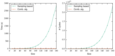
Figure 9: Running time and number of CPU cycles used by the sampling-based algorithm and the combinatorial adaptive seeding algorithm for different sizes of the core set.

Combinatorial vs. LP algorithm. We now compare the running time of the LP-based approach and the combinatorial approach for different instance sizes.

Figure 10 shows the running time and number of CPU cycles used by the LP algorithm and the combinatorial algorithm as a function of the network size $n$. The varying size of the network was obtained by randomly sampling a varying fraction of core set users and then trimming the social graph by only keeping friends of this random sample on the second stage. The LP solver used was CLP [1].

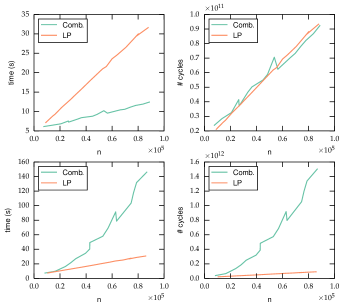
Figure 10: Running time and number of CPU cycles of the combinatorial algorithm and the LP algorithm as a function of the number of nodes $n$. First row with budget $k=100$, second row with budget $k=500$.

We observe that for a small value of the budget $k$ (first row of Figure 10), the combinatorial algorithm outperforms the LP algorithm. When $k$ becomes large (second row of Figure 10), the LP algorithm becomes faster. This can be explained by the $k^{2}$ factor in the running time of the combinatorial algorithm (see Proposition 5). Even though the asymptotic guarantee of the combinatorial algorithm should theoretically outperform the LP-based approach for large $n$, we were not able to observe it for our instance sizes. In practice, one can choose which of the two algorithms to apply depending on the relative sizes of $k$ and $n$.

6 Related work

Influence maximization was introduced by Domingos and Richardson [7, 24], formulated by Kempe, Kleinberg and Tardos [13, 14], and has been extensively studied since [22, 5, 19, 22, 5, 21, 4]. The main result in [13, 14] is a characterization of influence processes as submodular functions, which implies good approximation guarantees for the influence maximization problem. In [8], the authors look at the special case of the voter model and design efficient algorithms in this setting.

Our two-stage model for influence maximization is related to the field of stochastic optimization where problems are commonly solved using the sample average approximation method [15]. Golovin and Krause [11] study a stochastic sequential submodular maximization problem where at each step an element is chosen, its realization is revealed and the next decision is made. We note that contrary to adaptive seeding, the decision made at a given stage does not affect the following stages as the entire set of nodes is available as potential seeds at every stage.

Appendix A Adaptivity proofs

Proof A.1 (of Proposition 1).

We will first show that the optimal adaptive policy can be interpreted as a non-adaptive policy. Let $S$ be the optimal adaptive solution and define $\delta_{R}:\mathcal{N}(X)\mapsto\{0,1\}$:

$$\delta_{R}(u)\equiv\begin{cases}1&\text{if }u\in\operatorname*{argmax}\big{\{}f(T);\;T\subseteq R,\;|T|\leq k-|S|\big{\}}\\ 0&\text{otherwise}\end{cases},$$

one can write

$$\begin{split}\sum_{R\subseteq\mathcal{N}(S)}p_{R}\max_{\begin{subarray}{c}T\subseteq R\\ |T|\leq k-|S|\end{subarray}}f(T)&=\sum_{R\subseteq\mathcal{N}(S)}p_{R}\sum_{u\in\mathcal{N}(X)}\delta_{R}(u)w_{u}\\ &=\sum_{u\in\mathcal{N}(X)}w_{u}\sum_{R\subseteq\mathcal{N}(S)}p_{R}\delta_{R}(u).\end{split}$$

Let us now define for $u\in\mathcal{N}(X)$:

$$q_{u}\equiv\begin{cases}\sum_{R\subseteq\mathcal{N}(S)}\frac{p_{R}}{p_{u}}\delta_{R}(u)&\text{if }p_{u}\neq 0\\ 0&\text{otherwise}\end{cases}.$$

This allows us to write:

$$\sum_{R\subseteq\mathcal{N}(S)}p_{R}\max_{\begin{subarray}{c}T\subseteq R\\ |T|\leq k-|S|\end{subarray}}f(T)=\sum_{u\in\mathcal{N}(X)}p_{u}q_{u}w_{u}=F(\mathbf{p}\circ\mathbf{q})$$

where the last equality is obtained from (4) by successively using the linearity of the expectation and the linearity of $f$.

Furthermore, observe that $q_{u}\in[0,1]$, $q_{u}=0$ if $u\notin\mathcal{N}(S)$ and:

$$\begin{split}|S|+\sum_{u\in\mathcal{N}(X)}p_{u}q_{u}&=|S|+\sum_{R\subseteq\mathcal{N}(S)}p_{R}\sum_{u\in\mathcal{N}(X)}\delta_{R}(u)\\ &\leq|S|+\sum_{R\subseteq\mathcal{N}(S)}p_{R}(k-|S|)\leq k\end{split}$$

Hence, $(S,\mathbf{q})\in\mathcal{F}_{NA}$. In other words, we have written the optimal adaptive solution as a relaxed non-adaptive solution. This conclude the proof of the proposition.

Proof A.2 (of Proposition 2).

Using the definition of $\mathrm{A}(S)$, one can write:

$$\mathrm{A}(S)=\sum_{R\subseteq\mathcal{N}(S)}p_{R}\max_{\begin{subarray}{c}T\subseteq R\\ |T|\leq k-|S|\end{subarray}}f(T)\geq\sum_{R\subseteq\mathcal{N}(S)}p_{R}\mathbf{E}\big{[}f(I)\big{]}$$

where the inequality comes from the fact that $I$ is a feasible random set: $|I|\leq k-|S|$, hence the expected value of $f(I)$ is bounded by the maximum of $f$ over feasible sets.

Equation (5) then implies:

$$\mathrm{A}(S)\geq(1-\varepsilon)\sum_{R\subseteq\mathcal{N}(S)}p_{R}F(\mathbf{q})=(1-\varepsilon)F(\mathbf{p}\circ\mathbf{q}).$$ (11)

Equation (11) holds for any $\varepsilon\geq 0$. In particular, for $\varepsilon$ smaller than $\inf_{S\neq T}|A(S)-A(T)|$, we obtain that $\mathrm{A}(S)\geq F(\mathbf{p}\circ\mathbf{q})$. Note that such a $\varepsilon$ is at most polynomially small in the size of the instance. $(S,\mathbf{q})$ is an $\alpha$-approximate non adaptive solution, hence $F(\mathbf{p}\circ\mathbf{q})\geq\alpha\mathrm{OPT}_{NA}$. We can then conclude by applying Proposition 1.

Appendix B Algorithms Proofs

We first discuss the NP-hardness of the problem.

NP-Hardness. In contrast to standard influence maximization, adaptive seeding is already NP-Hard even for the simplest cases. In the case when $f(S)=|S|$ and all probabilities equal one, the decision problem is whether given a budget $k$ and target value $\ell$ there exists a subset of $X$ of size $k-t$ which yields a solution with expected value of $\ell$ using $t$ nodes in $\mathcal{N}(X)$. This is equivalent to deciding whether there are $k-t$ nodes in $X$ that have $t$ neighbors in $\mathcal{N}(X)$. To see this is NP-hard, consider reducing from Set-Cover where there is one node $i$ for each input set $T_{i}$, $1\leq i\leq n$, with $\mathcal{N}(i)=T_{i}$ and integers $k,\ell$, and the output is “yes” if there is a family of $k$ sets in the input which cover at least $\ell$ elements, and “no” otherwise.

B.1 LP-based approach

In the LP-based approach we rounded the solution using the pipage rounding method. We discuss this with greater detail here.

Pipage Rounding. The pipage rounding method [2] is a deterministic rounding method that can be applied to a variety of problems. In particular, it can be applied to LP-relaxations of the Max-K-Cover problem where we are given a family of sets that cover elements of a universe and the goal is to find $k$ subsets whose union has the maximal cardinality. The LP-relaxation is a fractional solution over subsets, and the pipage rounding procedure then rounds the allocation in linear time, and the integral solution is guaranteed to be within a factor of $(1-1/e)$ of the fractional solution. We make the following key observation: for any given q, one can remove all elements in $\mathcal{N}(X)$ for which $q_{u}=0$, without changing the value of any solution $(\boldsymbol{\lambda},\textbf{q})$. Our rounding procedure can therefore be described as follows: given a solution $(\boldsymbol{\lambda},\textbf{q})$ we remove all nodes $u\in\mathcal{N}(X)$ for which $q_{u}=0$, which leaves us with a fractional solution to a (weighted) version of the Max-K-Cover problem where nodes in $X$ are the sets and the universe is the set of weighted nodes in $\mathcal{N}(X)$ that were not removed. We can therefore apply pipage rounding and lose only a factor of $(1-1/e)$ in quality of the solution.

B.2 Combinatorial Algorithm

We include the missing proofs from the combinatorial algorithm section. The scalability and implementation in MapReduce are discussed in this section as well.

Proof B.1 (of Lemma 2).

W.l.o.g we can rename and order the pairs in $T$ so that $w_{1}\geq w_{2}\geq\ldots\geq w_{m}$. Then, $\mathcal{O}(T,b)$ has the following simple piecewise linear expression:

$$\mathcal{O}(T,b)=\begin{cases}bw_{1}&\text{if }0\leq b<p_{1}\\ \displaystyle\sum_{k=1}^{i-1}p_{k}(w_{k}-w_{i})+bw_{i}&\displaystyle\text{if }0\leq b-\sum_{k=1}^{i-1}p_{k}<p_{i}\\ \displaystyle\sum_{k=1}^{m}p_{k}w_{k}&\displaystyle\text{if }b\geq\sum_{i=1}^{m}p_{k}\par\end{cases}$$

Let us define for $t\in\mathbf{R}^{+}$, $n(t)\equiv\inf\Big{\{}i\text{ s.t. }\sum_{k=1}^{i}p_{k}>t\Big{\}}$ with $n(t)=+\infty$ when the set is empty. In particular, note that $x\mapsto n(t)$ is non-decreasing. Denoting $\partial_{+}\mathcal{O}_{T}$ the right derivative of $\mathcal{O}(T,\cdot)$, one can write $\partial_{+}\mathcal{O}_{T}(t)=w_{n(t)}$, with the convention that $w_{\infty}=0$.

Writing $i\equiv\sup\Big{\{}j\text{ s.t. }w_{j}\geq w_{x}\Big{\}}$, it is easy to see that $\partial_{+}\mathcal{O}_{T\cup\{x\}}\geq\partial_{+}\mathcal{O}_{T}$. Indeed:

1. if $n(t)\leq i$ then $\partial_{+}\mathcal{O}_{T\cup\{x\}}(t)=\partial_{+}\mathcal{O}_{T}(t)=w_{n(t)}$.

2. if $n(t)\geq i+1$ and $n(t-c)\leq i$ then $\partial_{+}\mathcal{O}_{T\cup\{x\}}(t)=w_{x}\geq w_{n(t)}=\partial_{+}\mathcal{O}_{T}(t)$.

3. if $n(t-c)\geq i+1$, then $\partial_{+}\mathcal{O}_{T\cup\{x\}}=w_{n(t-c)}\geq w_{n(t)}=\partial_{+}\mathcal{O}_{T}(t)$.

Let us now consider $b$ and $c$ such that $b\leq c$. Then, using the integral representation of $\mathcal{O}(T\cup\{x\},\cdot)$ and $\mathcal{O}(T,\cdot)$, we get:

$$\mathcal{O}(T\cup\{x\},c)-\mathcal{O}(T\cup\{x\},b)=\int_{b}^{c}\partial_{+}\mathcal{O}_{T\cup\{x\}}(t)dt\\ \geq\int_{b}^{c}\partial_{+}\mathcal{O}_{T}(t)dt=\mathcal{O}(T,c)-\mathcal{O}(T,b)$$

Re-ordering the terms, $\mathcal{O}(T\cup\{x\},c)-\mathcal{O}(T,c)\geq\mathcal{O}(T\cup\{x\},b)-\mathcal{O}(T,b)$ which concludes the proof of the lemma.

Proof B.2 (of Lemma 3).

Let $T\subseteq\mathcal{N}(X)$ and $x,y\in\mathcal{N}(X)\setminus T$. Using the second-order characterization of submodular functions, it suffices to show that:

$$\mathcal{O}(T\cup\{x\},b)-\mathcal{O}(T,b)\geq\mathcal{O}(T\cup\{y,x\},b)-\mathcal{O}(T\cup\{y\},b)$$

We distinguish two cases based on the relative position of $w_{x}$ and $w_{y}$. The following notations will be useful: $S_{T}^{x}\equiv\big{\{}u\in T\text{ s.t. }w_{x}\leq w_{u}\big{\}}$ and $P_{T}^{x}\equiv T\setminus S_{T}^{x}$.

Case 1: If $w_{y}\geq w_{x}$, then one can write:

$$\mathcal{O}(T\cup\{y,x\},b)=\mathcal{O}(P_{T}^{y}\cup\{y\},b_{1})+\mathcal{O}(S_{T}^{y}\cup\{x\},b_{2})$$

$$\mathcal{O}(T\cup\{y\},b)=\mathcal{O}(P_{T}^{y}\cup\{y\},b_{1})+\mathcal{O}(S_{T}^{y},b_{2})$$

where $b_{1}$ is the fraction of the budget $b$ spent on $P_{T}^{y}\cup\{y\}$ and $b_{2}=b-b_{1}$.

Similarly:

$$\mathcal{O}(T\cup\{x\},b)=\mathcal{O}(P_{T}^{y},c_{1})+\mathcal{O}(S_{T}^{y}\cup\{x\},c_{2})$$

$$\mathcal{O}(T,b)=\mathcal{O}(P_{T}^{y},c_{1})+\mathcal{O}(S_{T}^{y},c_{2})$$

where $c_{1}$ is the fraction of the budget $b$ spent on $P_{T}^{y}$ and $c_{2}=b-c_{1}$.

Note that $b_{1}\geq c_{1}$: an optimal solution will first spent as much budget as possible on $P_{T}^{y}\cup\{y\}$ before adding elements in $S_{T}^{y}\cup\{x\}$.

In this case:

$$\begin{split}\mathcal{O}(T\cup\{x\},b)-\mathcal{O}(T,b)&=\mathcal{O}(S_{T}^{y}\cup\{x\},c_{2})+\mathcal{O}(S_{T}^{y},c_{2})\\ &\geq\mathcal{O}(S_{T}^{y}\cup\{x\},b_{2})+\mathcal{O}(S_{T}^{y},b_{2})\\ &=\mathcal{O}(T\cup\{y,x\},b)-\mathcal{O}(T\cup\{y\},b)\end{split}$$

where the inequality comes from Lemma 2 and $c_{2}\geq b_{2}$.

Case 2: If $w_{x}>w_{y}$, we now decompose the solution on $P_{T}^{x}$ and $S_{T}^{x}$:

$$\mathcal{O}(T\cup\{x\},b)=\mathcal{O}(P_{T}^{x}\cup\{x\},b_{1})+\mathcal{O}(S_{T}^{x},b_{2})$$

$$\mathcal{O}(T,b)=\mathcal{O}(P_{T}^{x},c_{1})+\mathcal{O}(S_{T}^{x},c_{2})$$

$$\mathcal{O}(T\cup\{y,x\},b)=\mathcal{O}(P_{T}^{x}\cup\{x\},b_{1})+\mathcal{O}(S_{T}^{x}\cup\{y\},b_{2})$$

$$\mathcal{O}(T\cup\{y\},b)=\mathcal{O}(P_{T}^{x},c_{1})+\mathcal{O}(S_{T}^{x}\cup\{y\},c_{2})$$

with $b_{1}+b_{2}=b$, $c_{1}+c_{2}=b$ and $b_{2}\leq c_{2}$.

In this case again:

$$\mathcal{O}(T\cup\{x\},b)-\mathcal{O}(T,b)=\mathcal{O}(S_{T}^{x},b_{2})-\mathcal{O}(S_{T}^{x},c_{2})\\ \geq\mathcal{O}(S_{T}^{x}\cup\{y\},b_{2})-\mathcal{O}(S_{T}^{x}\cup\{y\},c_{2})\\ =\mathcal{O}(T\cup\{y,x\},b)-\mathcal{O}(T\cup\{y\},b)$$

where the inequality uses Lemma 2 and $c_{2}\geq b_{2}$.

In both cases, we were able to obtain the second-order characterization of submodularity. This concludes the proof of the lemma.

Proof B.3 (of Proposition 3).

Let us consider $S$ and $T$ such that $S\subseteq T\subseteq X$ and $x\in X\setminus T$. In particular, note that $\mathcal{N}(S)\subseteq\mathcal{N}(T)$.

Let us write $\mathcal{N}(S\cup\{x\})=\mathcal{N}(S)\cup R$ with $\mathcal{N}(S)\cap R=\emptyset$ and similarly, $\mathcal{N}(T\cup\{x\})=\mathcal{N}(T)\cup R^{\prime}$ with $\mathcal{N}(T)\cap R^{\prime}=\emptyset$. It is clear that $R^{\prime}\subseteq R$. Writing $R^{\prime}=\{u_{1},\ldots,u_{k}\}$:

$$\mathcal{O}(\mathcal{N}(T\cup\{x\}),b)-\mathcal{O}(\mathcal{N}(T),b)\\ =\sum_{i=1}^{k}\mathcal{O}(\mathcal{N}(T)\cup\{u_{1},\ldots u_{i}\},b)-\mathcal{O}(\mathcal{N}(T)\cup\{u_{1},\ldots u_{i-1}\},b)\\ \leq\sum_{i=1}^{k}\mathcal{O}(\mathcal{N}(S)\cup\{u_{1},\ldots u_{i}\},b)-\mathcal{O}(\mathcal{N}(S)\cup\{u_{1},\ldots u_{i-1}\},b)\\ =\mathcal{O}(\mathcal{N}(S)\cup R^{\prime},b)-\mathcal{O}(\mathcal{N}(S),b)$$

where the inequality comes from the submodularity of $\mathcal{O}(\cdot,b)$ proved in Lemma 3. This same function is also obviously set-increasing, hence:

$$\mathcal{O}(\mathcal{N}(S)\cup R^{\prime},b)-\mathcal{O}(\mathcal{N}(S),b)\\ \leq\mathcal{O}(\mathcal{N}(S)\cup R,b)-\mathcal{O}(\mathcal{N}(S),b)\\ =\mathcal{O}(\mathcal{N}(S\cup\{x\}),b)-\mathcal{O}(\mathcal{N}(S),b)$$

This concludes the proof of the proposition.

Proof B.4 (of Proposition 4).

We simply note that the content of the outer for loop on line 2 of Algorithm 1 is the greedy submodular maximization algorithm of [23]. Since $\mathcal{O}(\mathcal{N}(\cdot),t)$ is submodular (Proposition 3), this solves the inner $\max$ in (10) with an approximation ratio of $(1-1/e)$. The outer for loop then computes the outer $\max$ of (10).

As a consequence, Algorithm 1 computes a $(1-1/e)$-approximate non-adaptive solution. We conclude by applying Proposition 2.

B.3 Parallelization

As discussed in the body of the paper, the algorithm can be parallelized across $k$ different machines, each one computing an approximation for a fixed budget $k-t$ in the first stage and $t$ in the second. A slightly more sophisticated approach is to consider only $\log n$ splits: $(1,k-1),(2,k-2),\ldots,(2^{\lfloor\log n\rfloor},1)$ and then select the best solution from this set. It is not hard to see that in comparison to the previous approach, this would reduce the approximation guarantee by a factor of at most 2: if the optimal solution is obtained by spending $t$ on the first stage and $k-t$ in the second stage, then since $t\leq 2\cdot 2^{\lfloor\log t\rfloor}$ the solution computed for $(2^{\lfloor\log t\rfloor},k-2^{\lfloor\log t\rfloor})$ will have at least half that value. More generally, for any $\epsilon>0$ one can parallelize over $\log_{1+\epsilon}n$ machines at the cost of losing a factor of $(1+\epsilon)$ in the approximation guarantee.

B.4 Implementation in MapReduce

As noted in Section 4.2, lines 4 to 7 of Algorithm 1 correspond to the greedy heuristic of [23] applied to the submodular function $f_{t}(S)\equiv\mathcal{O}\big{(}\mathcal{N}(S),t\big{)}$. A variant of this heuristic, namely the $\varepsilon$-greedy heuristic, combined with the Sample&Prune method of [16] allows us to write a MapReduce version of Algorithm 1. The resulting algorithm is described in Algorithm 2

Algorithm 2 Combinatorial algorithm, MapReduce

1:  $S\leftarrow\emptyset$

2:  for $t=1$ to $k-1$ do

3:        $S_{t}\leftarrow\emptyset$

4:        for $i=1$ to $\log_{1+\varepsilon}\Delta$ do

5:              $U\leftarrow X$, $S^{\prime}\leftarrow\emptyset$

6:              while $|U|>0$ do

7:                    $R\leftarrow$ sample from $U$ w.p. $\min\left(1,\frac{\ell}{|U|}\right)$

8:                    while $|R|>0$ or $|S_{t}\cup S^{\prime}|<k$ do

9:                          $x\leftarrow$ some element from $R$

10:                          if $\nabla f_{t}(S_{t}\cup S^{\prime},x)\geq\frac{\Delta}{(1+\varepsilon)^{i}}$ then

11:                                $S^{\prime}\leftarrow S^{\prime}\cup\{x\}$

12:                          end if

13:                          $R\leftarrow R\setminus\{x\}$

14:                    end while

15:                    $S_{t}\leftarrow S_{t}\cup S^{\prime}$

16:                    $U\leftarrow\{x\in U\,|\,\nabla f_{t}(S_{t},x)\geq\frac{\Delta}{(1+\varepsilon)^{i}}\}$

17:              end while

18:        end for

19:        if $\mathcal{O}(\mathcal{N}(S_{t}),t)>\mathcal{O}(\mathcal{N}(S),k-|S|)$ then

20:              $S\leftarrow S_{t}$

21:        end if

22:  end for

23:  return  $S$

We denoted by $\nabla f_{t}(S,x)$ the marginal increment of $x$ to the set $S$ for the function $f_{t}$, $\nabla f_{t}(S,x)=f_{t}(S\cup\{x\})-f_{t}(S)$. $\Delta$ is an upper bound on the marginal contribution of any element. In our case, $\Delta=\max_{u\in\mathcal{N}(X)}w_{u}$ provides such an upper bound. The sampling in line 7 selects a small enough number of elements that the while loop from lines 8 to 14 can be executed on a single machine. Furthermore, lines 7 and 16 can be implemented in one round of MapReduce each.

The approximation ratio of Algorithm 2 is $1-\frac{1}{e}-\varepsilon$. The proof of this result as well as the optimal choice of $\ell$ follow from Theorem 10 in [16].

References

- [1] https://projects.coin-or.org/Clp.
- [2] A. A. Ageev and M. Sviridenko. Pipage rounding: A new method of constructing algorithms with proven performance guarantee. J. Comb. Optim., 8(3):307–328, 2004.
- [3] E. Bakshy, J. M. Hofman, W. A. Mason, and D. J. Watts. Everyone’s an influencer: quantifying influence on twitter. In WSDM, 2011.
- [4] C. Borgs, M. Brautbar, J. Chayes, and B. Lucier. Maximizing social influence in nearly optimal time. In SODA, volume 14. SIAM, 2014.
- [5] N. Chen. On the approximability of influence in social networks. In SODA, pages 1029–1037, 2008.
- [6] J. Cheng, L. Adamic, P. A. Dow, J. M. Kleinberg, and J. Leskovec. Can cascades be predicted? WWW ’14, pages 925–936, New York, NY, USA, 2014. ACM.
- [7] P. Domingos and M. Richardson. Mining the network value of customers. In KDD, pages 57–66, 2001.
- [8] E. Even-Dar and A. Shapira. A note on maximizing the spread of influence in social networks. In WINE, pages 281–286, 2007.
- [9] S. L. Feld. Why your friends have more friends than you do. American Journal of Sociology, pages 1464–1477, 1991.
- [10] S. Goel, D. J. Watts, and D. G. Goldstein. The structure of online diffusion networks. In EC ’12, Valencia, Spain, June 4-8, 2012, pages 623–638, 2012.
- [11] D. Golovin and A. Krause. Adaptive submodularity: Theory and applications in active learning and stochastic optimization. Journal of Artificial Intelligence Research, 42(1):427–486, 2011.
- [12] R. A. Holley and T. M. Liggett. Ergodic theorems for weakly interacting infinite systems and the voter model. The annals of probability, pages 643–663, 1975.
- [13] D. Kempe, J. M. Kleinberg, and É. Tardos. Maximizing the spread of influence through a social network. In KDD, pages 137–146, 2003.
- [14] D. Kempe, J. M. Kleinberg, and É. Tardos. Influential nodes in a diffusion model for social networks. In ICALP, pages 1127–1138, 2005.
- [15] A. J. Kleywegt, A. Shapiro, and T. Homem-de Mello. The sample average approximation method for stochastic discrete optimization. SIAM Journal on Optimization, 12(2):479–502, 2002.
- [16] R. Kumar, B. Moseley, S. Vassilvitskii, and A. Vattani. Fast greedy algorithms in mapreduce and streaming. In G. E. Blelloch and B. Vöcking, editors, SPAA 2013, pages 1–10. ACM, 2013.
- [17] S. Lattanzi and Y. Singer. The power of random neighbors in social networks. WSDM 2015.
- [18] J. Leskovec, D. Chakrabarti, J. M. Kleinberg, and C. Faloutsos. Realistic, mathematically tractable graph generation and evolution, using kronecker multiplication. In PKDD 2005, volume 3721 of Lecture Notes in Computer Science, pages 133–145. Springer, 2005.
- [19] J. Leskovec, A. Krause, C. Guestrin, C. Faloutsos, J. M. VanBriesen, and N. S. Glance. Cost-effective outbreak detection in networks. In KDD, pages 420–429, 2007.
- [20] J. Leskovec and A. Krevl. SNAP Datasets: Stanford large network dataset collection. http://snap.stanford.edu/data, June 2014.
- [21] M. Mathioudakis, F. Bonchi, C. Castillo, A. Gionis, and A. Ukkonen. Sparsification of influence networks. In KDD, 2011.
- [22] E. Mossel and S. Roch. On the submodularity of influence in social networks. In STOC, pages 128–134, 2007.
- [23] G. L. Nemhauser, L. A. Wolsey, and M. L. Fisher. An analysis of approximations for maximizing submodular set functions—i. Mathematical Programming, 14(1):265–294, 1978.
- [24] M. Richardson and P. Domingos. Mining knowledge-sharing sites for viral marketing. In KDD, pages 61–70, 2002.
- [25] M. Richardson and P. Domingos. Mining knowledge-sharing sites for viral marketing. In KDD, pages 61–70. ACM, 2002.
- [26] L. Seeman and Y. Singer. Adaptive seeding in social networks. In FOCS, 2013.
- [27] J. Vondrák, C. Chekuri, and R. Zenklusen. Submodular function maximization via the multilinear relaxation and contention resolution schemes. In STOC, pages 783–792. ACM, 2011.
- [28] J. Yang and S. Counts. Predicting the speed, scale, and range of information diffusion in twitter. In ICWSM, 2010.
- [29] T. R. Zaman, R. Herbrich, J. V. Gael, and D. Stern. Predicting information spreading in twitter, 2010.