Class Probability Estimation via Differential Geometric Regularization

Abstract

We study the problem of supervised learning for both binary and multiclass classification from a unified geometric perspective. In particular, we propose a geometric regularization technique to find the submanifold corresponding to a robust estimator of the class probability $P(y|\boldsymbol{x}).$ The regularization term measures the volume of this submanifold, based on the intuition that overfitting produces rapid local oscillations and hence large volume of the estimator. This technique can be applied to regularize any classification function that satisfies two requirements: firstly, an estimator of the class probability can be obtained; secondly, first and second derivatives of the class probability estimator can be calculated. In experiments, we apply our regularization technique to standard loss functions for classification, our RBF-based implementation compares favorably to widely used regularization methods for both binary and multiclass classification.

1 Introduction

In supervised learning for classification, the idea of regularization seeks a balance between a perfect description of the training data and the potential for generalization to unseen data. Most regularization techniques are defined in the form of penalizing some functional norms. For instance, one of the most successful classification methods, the support vector machine (SVM) (Vapnik, 1998; Schölkopf & Smola, 2002) and its variants (Bartlett et al., 2006; Steinwart, 2005), use a RKHS norm as a regularizer. While functional norm based regularization is widely-used in machine learning, we feel that there is important local geometric information overlooked by this approach.

In many real world classification problems, if the feature space is meaningful, then all samples that are locally within a small enough neighborhood of a training sample should have class probability $P(y|\boldsymbol{x})$ similar to the training sample. For instance, a small enough perturbation of RGB values at some pixels of a human face image should not change dramatically the likelihood of correct identification of this image during face recognition. However, such “small local oscillations” of the class probability are not explicitly incorporated by penalizing commonly used functional norms. For instance, as reported by Goodfellow et al. (2014), linear models and their combinations can be easily fooled by hardly perceptible perturbations of a correctly predicted image, even though a $L2$ regularizer is adopted.

Geometric regularization techniques have also been studied in machine learning. Belkin et al. (2006) employed geometric regularization in the form of the $L2$ norm of the gradient magnitude supported on a manifold. This approach exploits the geometry of the marginal distribution $P(\boldsymbol{x})$ for semi-supervised learning, rather than the geometry of the class probability $P(y|\boldsymbol{x})$. Other related geometric regularization methods are motivated by the success of level set methods in image segmentation (Cai & Sowmya, 2007; Varshney & Willsky, 2010) and Euler’s Elastica in image processing (Lin et al., 2012, 2015). In particular, the Level Learning Set (Cai & Sowmya, 2007) combines a counting function of training samples and a geometric penalty on the surface area of the decision boundary. The Geometric Level Set (Varshney & Willsky, 2010) generalizes this idea to standard empirical risk minimization schemes with margin-based loss. Along this line, the Euler’s Elastica Model (Lin et al., 2012, 2015) proposes a regularization technique that penalizes both the gradient oscillations and the curvature of the decision boundary. However, all three methods focus on the geometry of the decision boundary supported in the domain of the feature space, and the “small local oscillation” of the class probability is not explicitly addressed.

In this work, we argue that the “small local oscillation” of the class probability actually lies in the product space of the feature domain and the probabilistic output space, and can be characterized by the geometry of a submanifold in this product space corresponding to the class probability. Let $\boldsymbol{f}:\mathcal{X}\to\Delta^{L-1}$ be a class probability estimator, where $\mathcal{X}$ is the feature space and $\Delta^{L-1}$ is the probabilistic simplex for $L$ classes. From a geometric perspective, if we regard $\{(\boldsymbol{x},\boldsymbol{f}(\boldsymbol{x}))|\boldsymbol{x}\in\mathcal{X}\}$, the functional graph (in the geometric sense) of $\boldsymbol{f}$, as a submanifold in $\mathcal{X}\times\Delta^{L-1}$, then “small local oscillations” can be measured by the local flatness of this submanifold.

In our approach, the learning process can be viewed as a submanifold fitting problem that is solved by a geometric flow method. In particular, our approach finds a submanifold by iteratively fitting the training samples in a curvature or volume decreasing manner without any a priori assumptions on the geometry of the submanifold in $\mathcal{X}\times\Delta^{L-1}$. We use gradient flow methods to find an optimal direction, i.e. at each step we find the vector field pointing in the optimal direction to move $\boldsymbol{f}$. As we will see in the next section, this regularization approach naturally handles binary and multiclass classification in a unified way, while previous decision boundary based techniques (and most functional regularization approaches) are originally designed for binary classification, and rely on “one versus one”, “one versus all” or more efficiently a binary coding strategy (Varshney & Willsky, 2010) to generalize to multiclass case.

In experiments, a radial basis function (RBF) based implementation of our formulation compares favorably to widely used binary and multiclass classification methods on datasets from the UCI repository and real-world datasets including the Flickr Material Database (FMD) and the MNIST Database of handwritten digits.

In summary, our contributions are:

• A geometric perspective on overfitting and a regularization approach that exploits the geometry of a robust class probability estimator for classification,

• A unified gradient flow based algorithm for both binary and multiclass classification that can be applied to standard loss functions, and

• A RBF-based implementation that achieves promising experimental results.

2 Method Overview

In our work, we propose a regularization scheme that exploits the geometry of a robust class probability estimator and suggest a gradient flow based approach to solve for it. In the follow, we will describe our approach. Related mathematical notation is summarized in Table 2.

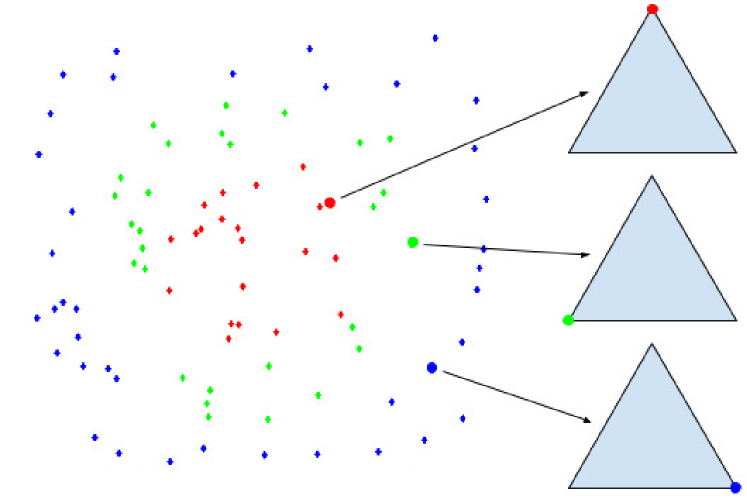
Figure 1: Example of three-class learning, i.e., $L=3$, where the input space $\mathcal{X}$ is $2d$. Training samples of the three classes are marked with red, green and blue dots respectively. The class label for each training sample corresponds to a vertex of the simplex $\Delta^{L-1}$. As a result, each mapped training point $(\boldsymbol{x}_{i},\boldsymbol{z}_{i})$ lies on one face (corresponding to its label $y_{i}$) of the space $\cal X\times$$\Delta^{2}$.

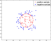
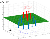
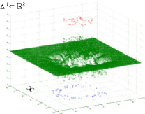
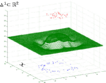
$(a)$	$(b)$	$(c)$	$(d)$

Figure 2: Example of binary learning via gradient flow. As shown in $(a),$ the feature space $\cal X$ is $2d$, training points are sampled uniformly within the region $[-15,15]\times[-15,15]$, and labeled by the function $y=\rm sign(10-\|\boldsymbol{x}\|_{2})$ (the red circle). In the initialization step, shown in $(b),$ positive and negative training points map to the two faces of the space $\mathcal{X}\times\Delta^{1}$ respectively. Our gradient flow method starts from a neutral function $\boldsymbol{f}_{0}\equiv\frac{1}{2}$ and moves towards the negative direction (red and blue arrows) of the penalty gradient $\nabla\mathcal{P}_{\boldsymbol{f}_{0}}.$ Figure $(c)$ shows the submanifold (${\rm gr}(\boldsymbol{f}_{1})$) one step after $(b)$. The submanifold then continues to evolve towards $-\nabla\mathcal{P}_{\boldsymbol{f}_{t}}$ step by step and the final output after convergence of the algorithm is shown in $(d).$

Following the probabilistic setting of classification, given a sample (feature) space $\mathcal{X}\subset\mathbb{R}^{N}$, a label space $\mathcal{Y}=\{1,\ldots,L\}$, and a finite training set of labeled samples $\mathcal{T}_{m}=\{(\boldsymbol{x}_{i},y_{i})\}_{i=1}^{m}$, where each training sample is generated i.i.d. from distribution $P$ over $\mathcal{X}\times\mathcal{Y}$, our goal is to find a $h_{\mathcal{T}_{m}}:\mathcal{X}\to\mathcal{Y}$ such that for any new sample $\boldsymbol{x}\in\mathcal{X}$, $h_{\mathcal{T}_{m}}$ predicts its label $\hat{y}=h_{\mathcal{T}_{m}}(\boldsymbol{x})$. The optimal generalization risk (Bayes risk) is achieved by the classifier $h^{*}(\boldsymbol{x})=\operatorname*{\arg\!\max}\{\eta^{\ell}(\boldsymbol{x}),\ell\in\mathcal{Y}\}$, where $\boldsymbol{\eta}=(\eta^{1},\ldots,\eta^{L})$ with $\eta^{\ell}:\mathcal{X}\to[0,1]$ being the $\ell^{\rm th}$ class probability, i.e. $\eta^{\ell}(\boldsymbol{x})=P(y=\ell|\boldsymbol{x})$.

Our regularization approach exploits the geometry of the class probability estimator, and can be regarded as a “hybrid” plug-in/ERM scheme (Audibert & Tsybakov, 2007). A regularized loss minimization problem is setup to find an estimator $\boldsymbol{f}:\mathcal{X}\to\Delta^{L-1}$, where $\Delta^{L-1}$ is the standard $(L-1)$-simplex in $\mathbb{R}^{L}$, and $\boldsymbol{f}=(f^{1},\ldots,f^{L})$ is an estimator of $\boldsymbol{\eta}$ with $f^{\ell}:\mathcal{X}\to[0,1]$. The estimator $\boldsymbol{f}$ is then “plugged-in” to get the classifier $h_{\boldsymbol{f}}(\boldsymbol{x})=\operatorname*{\arg\!\max}\{f^{\ell}(\boldsymbol{x}),\ell\in\mathcal{Y}\}.$

Figure 1 shows an example of the setup of our approach, for a synthetic three-class classification problem. The submanifold corresponding to estimator $\boldsymbol{f}$ is the graph (in the geometric sense) of $\boldsymbol{f}$: ${\rm gr}(\boldsymbol{f})=\{(\boldsymbol{x},f^{1}(\boldsymbol{x}),\ldots,f^{L}(\boldsymbol{x})):\boldsymbol{x}\in\mathcal{X}\}\subset\mathcal{X}\times\Delta^{L-1}$. We denote a point in the space $\mathcal{X}\times\Delta^{L-1}$ as $(\boldsymbol{x},\boldsymbol{z})=(x^{1},\ldots,x^{N},z^{1},\ldots,z^{L})$, where $\boldsymbol{x}\in\mathcal{X}$ and $\boldsymbol{z}\in\Delta^{L-1}.$ Then in this product space, a training pair $(\boldsymbol{x}_{i},y_{i}=\ell)$ naturally maps to the point $(\boldsymbol{x}_{i},\boldsymbol{z}_{i})=(\boldsymbol{x}_{i},0,\ldots,1,\ldots,0)$, with the one-hot vector $\boldsymbol{z}_{i}$ (with the $1$ in its $\ell$-th slot) at the vertex of $\Delta^{L-1}$ corresponding to $P(y=y_{i}|\boldsymbol{x})=1$.

We point out two properties of this geometric setup. Firstly, it inherently handles multiclass classification, with binary classification as a special case. Secondly, while the dimension of the ambient space, i.e. $\mathbb{R}^{N+L}$, depends on both the feature dimension $N$ and number of classes $L$, the intrinsic dimension of the submanifold ${\rm gr}(\boldsymbol{f})$ only depends on $N$.

2.1 Variational formulation

We want ${\rm gr}(\boldsymbol{f})$ to approach the mapped training points while remaining as flat as possible, so we impose a penalty on $\boldsymbol{f}$ consisting of an empirical loss term $\mathcal{P}_{\mathcal{T}_{m}}$ and a geometric regularization term $\mathcal{P}_{G}$. For $\mathcal{P}_{\mathcal{T}_{m}}$, we can choose either the widely-used cross-entropy loss function for multiclass classification or the simpler Euclidean distance function between the simplex coordinates of the graph point and the mapped training point. For $\mathcal{P}_{G}$, we would ideally consider an $L^{2}$ measure of the Riemann curvature of ${\rm gr}(\boldsymbol{f})$, as the vanishing of this term gives optimal (i.e., locally distortion free) diffeomorphisms from ${\rm gr}(\boldsymbol{f})$ to $\mathbb{R}^{N}.$ However, the Riemann curvature tensor takes the form of a combination of derivatives up to third order, and the corresponding gradient vector field is even more complicated and inefficient to compute in practice. As a result, we measure the graph’s volume, $\mathcal{P}_{G}(\boldsymbol{f})=\int_{{\rm gr}(\boldsymbol{f})}{\rm dvol}$, where ${\rm dvol}$ is the induced volume from the Lebesgue measure on the ambient space $\mathbb{R}^{N+L}$.

More precisely, we find the function that minimizes the following penalty $\mathcal{P}$:

$$\mathcal{P}=\mathcal{P}_{\mathcal{T}_{m}}+\lambda\mathcal{P}_{G}:\mathcal{M}={\rm Maps}(\mathcal{X},\Delta^{L-1})\to\mathbb{R}$$ (1)

on the set $\mathcal{M}$ of smooth functions from $\mathcal{X}$ to $\Delta^{L-1}$, where $\lambda$ is the tradeoff parameter between empirical loss and regularization. It is important to note that any relative scaling of the domain $\mathcal{X}$ will not affect the estimate of the class probability $\boldsymbol{\eta}$, as scaling will distort ${\rm gr}(\boldsymbol{f})$ but will not change the critical function estimating $\boldsymbol{\eta}$.

2.2 Gradient flow and geometric foundation

The standard technique for solving variational formulas is the Euler-Lagrange PDE. However, due to our geometric term $\mathcal{P}_{G}$, finding the minimal solutions of the Euler-Lagrange equations for $\mathcal{P}$ is difficult, instead, we solve for ${\rm argmin}\ \mathcal{P}$ using gradient flow in functional space $\mathcal{M}.$

A simple but intuitive simulated example of binary learning using gradient flow for our approach is given in Figure 2. For the explanation purposes only, we replace $\mathcal{M}$ with a finite dimensional Riemannian manifold $M$. Without loss of generality, we also assume that $\mathcal{P}$ is smooth, then it has a differential $d\mathcal{P}_{\boldsymbol{f}}:T_{\boldsymbol{f}}M\to\mathbb{R}$ for each $\boldsymbol{f}\in M$, where $T_{\boldsymbol{f}}M$ is the tangent space to $M$ at $\boldsymbol{f}$. Since $d\mathcal{P}_{\boldsymbol{f}}$ is a linear functional on $T_{\boldsymbol{f}}M$, there is a unique tangent vector, denoted $\nabla\mathcal{P}_{\boldsymbol{f}}$, such that $d\mathcal{P}_{\boldsymbol{f}}(\boldsymbol{v})=\langle\boldsymbol{v},\nabla\mathcal{P}_{\boldsymbol{f}}\rangle$ for all $\boldsymbol{v}\in T_{\boldsymbol{f}}M.$ $\nabla\mathcal{P}_{\boldsymbol{f}}$ points in the direction of maximal increase of $\mathcal{P}$ at $\boldsymbol{f}$. Thus, the solution of the negative gradient flow $d\boldsymbol{f}_{t}/dt=-\nabla\mathcal{P}_{\boldsymbol{f}_{t}}$ is a flow line of steepest descent starting at an initial $\boldsymbol{f}_{0}.$ For a dense open set of initial points, flow lines approach a local minimum of $\mathcal{P}$ at $t\to\infty.$ We always choose the initial function $\boldsymbol{f}_{0}$ to be the “neutral” choice $\boldsymbol{f}_{0}(\boldsymbol{x})\equiv(\frac{1}{L},\ldots,\frac{1}{L})$ which reasonably assigns equal conditional probability to all classes.

Similar gradient flow procedures are widely used in variational problems, such as level set methods (Osher & Sethian, 1988; Sethian, 1999), Mumford-Shah functional (Mumford & Shah, 1989), etc. In the classification literature, Varshney & Willsky (2010) were the first to use gradient flow methods for solving level set based energy functions, then followed by Lin et al. (2012, 2015) to solve Euler’s Elastica models. In our case, we are exploiting the geometry in the space $\mathcal{X}\times\Delta^{L-1},$ rather than standard vector spaces.

Since our gradient flow method is actually applied on the infinite dimensional manifold $\mathcal{M},$ we have to understand both the topology and the Riemannian geometry of $\mathcal{M}$. For the topology, we put the Fréchet topology on $\mathcal{M}^{\prime}={\rm Maps}(\mathcal{X},\mathbb{R}^{L})$, the set of smooth maps from $\mathcal{X}$ to $\mathbb{R}^{L}$, and take the induced topology on $\mathcal{M}.$ Intuitively speaking, two functions in $\mathcal{M}$ are close if the functions and all their partial derivatives are pointwise close. Since $\mathcal{M}$ is an open Fréchet submanifold with boundary inside the vector space $\mathcal{M}^{\prime}$, so as with an open set in Euclidean space, we can canonically identify $T_{\boldsymbol{f}}\mathcal{M}$ with $\mathcal{M}^{\prime}$. For the Riemannian metric, we take the $L^{2}$ metric on each tangent space $T_{\boldsymbol{f}}\mathcal{M}$: $\langle\phi_{1},\phi_{2}\rangle:=\int_{\mathcal{X}}\phi_{1}(\boldsymbol{x})\phi_{2}(\boldsymbol{x}){\rm dvol}_{\boldsymbol{x}}$, with $\phi_{i}\in\mathcal{M}^{\prime}$ and ${\rm dvol}_{\boldsymbol{x}}$ being the volume form of the induced Riemannian metric on the graph of $\boldsymbol{f}$. (Strictly speaking, the volume form is pulled back to $\mathcal{X}$ by $\boldsymbol{f}$, usually denoted by $\boldsymbol{f}^{*}{\rm dvol}$.)

The differential $d\mathcal{P}_{\boldsymbol{f}}$ is linear as above, and by a direct calculation, there is a unique tangent vector $\nabla\mathcal{P}_{\boldsymbol{f}}\in T_{\boldsymbol{f}}\mathcal{M}$ such that $d\mathcal{P}_{\boldsymbol{f}}(\phi)=\langle\nabla\mathcal{P}_{\boldsymbol{f}},\phi\rangle$ for all $\phi\in T_{\boldsymbol{f}}\mathcal{M}.$ Thus, we can construct the gradient flow equation. However, unlike the case of finite dimensions, the existence of flow lines is not automatic. Assuming the existence of flow lines, a generic initial point flows to a local minimum of $\mathcal{P}$. In any case, our RBF-based implementation in §3 mimicking gradient flow is well defined.

Note that we think of $\mathcal{X}$ as large enough so that the training data actually is sampled well inside $\mathcal{X}$. This allows us to treat $\mathcal{X}$ as a closed manifold in our gradient calculations, so that boundary effects can be ignored. A similar natural boundary condition is also adopted by previous work (Varshney & Willsky, 2010; Lin et al., 2012, 2015).

2.3 More on related work

There exist some other works that are related to some aspects of our work. Most notably, Sobolev regularization, involves functional norms of a certain number of derivatives of the prediction function. For instance, the manifold regularization (Belkin et al., 2006) mentioned in §1 uses a Sobolev regularization term,

$$\int_{x\in\mathcal{M}}\|\nabla_{\mathcal{M}}f\|^{2}dP(x),$$ (2)

where $f$ is a smooth function on manifold $\mathcal{M}.$ A discrete version of (2) corresponds to the graph Laplacian regularization (Zhou & Schölkopf, 2005). Lin et al. (2015) discussed in detail the difference between a Sobolev norm and a curvature-based norm for the purpose of exploiting the geometry of the decision boundary.

For our purpose, while imposing, say, a high Sobolev norm, will also lead to a flattening of the hypersurface ${\rm gr}(\boldsymbol{f})$, these norms are not specifically tailored to measuring the flatness of ${\rm gr}(\boldsymbol{f})$. In other words, a high Sobolev norm bound will imply the volume bound we desire, but not vice versa. As a result, imposing high Sobolev norm constraints (regardless of computational difficulties) overshrinks the hypothesis space from a learning theory point of view. In contrast, our regularization term (given in (11)) involves only the combination of first derivatives of $\boldsymbol{f}$ that specifically address the geometry behind the “small local oscillation” prior observed in practice.

Our training procedure for finding the optimal graph of a function is, in a general sense, also related to the manifold learning problem (Tenenbaum et al., 2000; Roweis & Saul, 2000; Belkin & Niyogi, 2003; Donoho & Grimes, 2003; Zhang & Zha, 2005; Lin & Zha, 2008). The most closely related work is (Donoho & Grimes, 2003), which seeks a flat submanifold of Euclidean space that contains a dataset. Again, there are key differences. Since the goal of (Donoho & Grimes, 2003) is dimensionality reduction, their manifold has high codimension, while our functional graph has codimension $L-1$, which may be as low as $1$. More importantly, we do not assume that the graph of our target function is a flat (or volume minimizing) submanifold, and we instead flow towards a function whose graph is as flat (or volume minimizing) as possible. In this regard, our work is related to a large body of literature on Morse theory in finite and infinite dimensions, and on mean curvature flow (Chen et al., 1999; Mantegazza, 2011).

3 Example Formulation: RBFs

We now illustrate our approach using an RBF representation of our estimator $\boldsymbol{f}.$ RBFs are also used by previous geometric classification methods (Varshney & Willsky, 2010; Lin et al., 2012, 2015).

Given values of $\boldsymbol{f}$ are probabilistic vectors, it is common to represent $\boldsymbol{f}$ as a “softmax” output of RBFs, i.e.

$$f^{j}=\frac{e^{h^{j}}}{\sum_{l=1}^{L}e^{h^{l}}}, \text{where }h^{j}=\sum_{i=1}^{m}a_{i}^{j}\varphi_{i}(\boldsymbol{x}),$$ (3)

$$\text{for }j=1,\ldots,L,$$

where $\varphi_{i}(\boldsymbol{x})=e^{-\frac{1}{c}\|\boldsymbol{x}-\boldsymbol{x}_{i}\|^{2}}$ is the RBF function centered at training sample $\boldsymbol{x}_{i}$, with kernel width parameter $c$.

Estimating $\boldsymbol{f}$ becomes an optimization problem for the $m\times L$ coefficient matrix $A=(a_{i}^{\ell})$. The following equation determines $A$:

$$\left[\boldsymbol{h}(\boldsymbol{x}_{1}),\ldots,\boldsymbol{h}(\boldsymbol{x}_{m})\right]^{T}=GA,\ \text{where }G_{ij}=\varphi_{j}(\boldsymbol{x}_{i}).$$ (4)

To plug this RBF representation into our gradient flow scheme, the gradient vector field $\nabla\mathcal{P}_{\boldsymbol{f}}$ is evaluated at each sample point $\boldsymbol{x}_{i}$, and $A$ is updated by

$$A\leftarrow A-\tau G^{-1}\left[\nabla\mathcal{P}_{\boldsymbol{h}}(\boldsymbol{x}_{1}),\ldots,\nabla\mathcal{P}_{\boldsymbol{h}}(\boldsymbol{x}_{m})\right]^{T},$$ (5)

where $\tau$ is the step-size parameter, and

$$\nabla\mathcal{P}_{\boldsymbol{h}}(\boldsymbol{x}_{i})=\left[\frac{\partial\boldsymbol{f}}{\partial\boldsymbol{h}}\right]_{\boldsymbol{x}_{i}}^{T}\nabla\mathcal{P}_{\boldsymbol{f}}(\boldsymbol{x}_{i}).$$ (6)

Here $\nabla\mathcal{P}_{\boldsymbol{h}}(\boldsymbol{x}_{i})$ denotes the gradient vector field w.r.t. $\boldsymbol{h}$ evaluated at $\boldsymbol{x}_{i},$ and the $L\times L$ Jacobian matrix $\left[\frac{\partial\boldsymbol{f}}{\partial\boldsymbol{h}}\right]_{\boldsymbol{x}_{i}}$ can be obtained in closed form from (3). In the following subsections, we give exact forms of the empirical penalty $\mathcal{P}_{\mathcal{T}_{m}}$ and the geometric penalty $\mathcal{P}_{G}$, and discuss the computation of $\nabla\mathcal{P}_{\boldsymbol{h}}$ for both penalty terms.

3.1 The empirical penalty $\mathcal{P}_{\mathcal{T}_{m}}$

We consider two widely-used loss functions for the empirical penalty term $\mathcal{P}_{\mathcal{T}_{m}}.$

Quadratic loss. Since $\mathcal{P}_{\mathcal{T}_{m}}$ measures the deviation of ${\rm gr}(\boldsymbol{f})$ from the mapped training points, it is natural to choose the quadratic function of the Euclidean distance in the simplex $\Delta^{L-1},$

$$\mathcal{P}_{\mathcal{T}_{m}}(\boldsymbol{f})=\sum_{i=1}^{m}\|\boldsymbol{f}(\boldsymbol{x}_{i})-\boldsymbol{z}_{i}\|^{2},$$ (7)

where $\boldsymbol{z}_{i}$ is the one-hot vector corresponding to the ground truth label of $\boldsymbol{x}_{i}$. The gradient vector w.r.t. $\boldsymbol{f}$ evaluated at $\boldsymbol{x}_{i}$ is

$$\nabla\mathcal{P}_{\mathcal{T}_{m},\boldsymbol{f}}(\boldsymbol{x}_{i})=2(\boldsymbol{f}(\boldsymbol{x}_{i})-\boldsymbol{z}_{i}).$$

The gradient vector w.r.t. $\boldsymbol{h}$ evaluated at $\boldsymbol{x}_{i}$ is

$$\nabla\mathcal{P}_{\mathcal{T}_{m},\boldsymbol{h}}(\boldsymbol{x}_{i})=2\left[\frac{\partial\boldsymbol{f}}{\partial\boldsymbol{h}}\right]^{T}_{\boldsymbol{x}_{i}}(\boldsymbol{f}(\boldsymbol{x}_{i})-\boldsymbol{z}_{i}),$$ (8)

evaluation of $\left[\frac{\partial\boldsymbol{f}}{\partial\boldsymbol{h}}\right]^{T}_{\boldsymbol{x}_{i}}$ is the same as in (6).

Cross-entropy loss. The cross-entropy loss function is also widely-used for probabilistic output in classification,

$$\mathcal{P}_{\mathcal{T}_{m}}(\boldsymbol{f})=-\sum_{i=1}^{m}\sum_{\ell=1}^{L}z_{i}^{\ell}\log f^{\ell}(\boldsymbol{x}_{i}),$$ (9)

whose gradient vector field w.r.t. $\boldsymbol{h}$ evaluated at $\boldsymbol{x}_{i}$ is

$$\nabla\mathcal{P}_{\mathcal{T}_{m},\boldsymbol{h}}(\boldsymbol{x}_{i})=\boldsymbol{f}(\boldsymbol{x}_{i})-\boldsymbol{z}_{i}.$$ (10)

3.2 The geometric penalty $\mathcal{P}_{G}$

As discussed in §2, we wish to penalize graphs for excessive curvature and we use the following function, which measures the volume of the ${\rm gr}(\boldsymbol{f})$:

$$\mathcal{P}_{G}(\boldsymbol{f})=\int_{{\rm gr}(\boldsymbol{f})}{\rm dvol}=\int_{{\rm gr}(\boldsymbol{f})}\sqrt{\det(g)}dx^{1}\ldots dx^{N},$$ (11)

where $g=(g_{ij})$ with $g_{ij}=\delta_{ij}+f^{a}_{i}f^{a}_{j},$ is the Riemmanian metric on ${\rm gr}(\boldsymbol{f})$ induced from the standard dot product on $\mathbb{R}^{N+L}.$ We use the summation convention on repeated indices. Note that this regularization term is clearly very different from the standard Sobolev norm of any order.

It is standard that $\nabla\mathcal{P}_{G}=-{\rm Tr\ II}\in\mathbb{R}^{N+L}$ on the space of all embeddings of $\mathcal{X}$ in $\mathbb{R}^{N+L}$. If we restrict to the submanifold of graphs of $\boldsymbol{f}\in\mathcal{M}^{\prime}$, it is easy to calculate that the gradient of geometric penalty (11) is

$$\nabla\mathcal{P}_{G,\boldsymbol{f}}=V_{G,\boldsymbol{f}}=-{\rm Tr\ II}^{L},$$ (12)

where ${\rm Tr\ II}^{L}$ denotes the last $L$ components of ${\rm Tr\ II}.$ Then the geometric gradient w.r.t. $\boldsymbol{h}$ is

$$\nabla\mathcal{P}_{G,\boldsymbol{h}}=V_{G,\boldsymbol{h}}=-\left[\frac{\partial\boldsymbol{f}}{\partial\boldsymbol{h}}\right]^{T}{\rm Tr\ II}^{L}.$$ (13)

Evaluation of $\left[\frac{\partial\boldsymbol{f}}{\partial\boldsymbol{h}}\right]$ and ${\rm Tr\ II}^{L}$ at $\boldsymbol{x}_{i}$ leads to $\nabla\mathcal{P}_{G,\boldsymbol{h}}(\boldsymbol{x}_{i}).$

The formulation given above is general in that it encompasses both the binary and the multiclass cases. For both cases, evaluation of $\left[\frac{\partial\boldsymbol{f}}{\partial\boldsymbol{h}}\right]$ at the training points is the same as that in (6), and evaluation of ${\rm Tr\ II}^{L}$ at any point $\boldsymbol{x}$ can be performed explicitly by the following theorem.

Theorem 1.

For $\boldsymbol{f}:\mathbb{R}^{N}\to\Delta^{L-1}$, ${\rm Tr\ II}^{L}$ for ${\rm gr}(\boldsymbol{f})$ is given by

$${\rm Tr\ II}^{L} = (g^{-1})^{ij}\biggl{(}f^{1}_{ji}-(g^{-1})^{rs}f^{a}_{rs}f^{a}_{i}f^{1}_{j},\ldots,$$ (14)

$$f^{L}_{ji}-(g^{-1})^{rs}f^{a}_{rs}f^{a}_{i}f^{L}_{j}\biggr{)},$$

where $f_{i}^{a},f_{ij}^{a}$ denote partial derivatives of $f^{a}$.

The proof is in Appendix A. Note that for our RBF representation (3), the partial derivatives $f_{i}^{a},f_{ij}^{a}$ can be easily obtained in closed form.

Simplex constraint. The class probability estimators $\boldsymbol{f}:X\to\Delta^{L-1}$ always takes values in $\Delta^{L-1}\subset\mathbb{R}^{L}$. While this constraint is automatically satisfied for the flow of the empirical gradient vector formula (8) and (10), it may fail for the flow of geometric gradient vector formula (12). There are two ways to enforce this constraint for the geometric gradient vector field. First, since our initial function $\boldsymbol{f}_{0}$ takes values at the center of $\Delta^{L-1}$, we can orthogonally project the geometric gradient vector $V_{G,\boldsymbol{f}}$ to $V_{G,\boldsymbol{f}}^{\prime}$ in the tangent space $Z=\{(y^{1},\ldots,y^{L})\in\mathbb{R}^{L}:\sum_{\ell=1}^{L}y^{\ell}=0\}$ of the simplex, and then scale $\tau V_{G,\boldsymbol{f}}^{\prime}$ ($\tau$ is the stepsize) to ensure that the range of the new $\boldsymbol{f}_{1}$ lies in $\Delta^{L-1}$. We then iterate. More simply, we can select $L-1$ of the $L$ components of $\boldsymbol{f}(\boldsymbol{x})$, call the new function $\boldsymbol{f}^{\prime}:\mathcal{X}\to R^{L-1}$, and compute the $(L-1)$-dimensional gradient vector $V_{G,\boldsymbol{f}^{\prime}}$ following (12) and (14). The omitted component of the desired $L$-gradient vector is determined by $-\sum_{\ell=1}^{L-1}V^{\ell}_{G,\boldsymbol{f}^{\prime}}$, by the definition of $Z$. Our implementation reported follows this second approach, where we choose the $(L-1)$ components of $\boldsymbol{f}$ by omitting the component corresponding to the class with least number of training samples.

3.3 Algorithm summary

Algorithm 1 gives a summary of the classifier learning procedure. Input to the algorithm is the training set $\mathcal{T}_{m},$ RBF kernel width $c$, trade-off parameter $\lambda$, and step-size parameter $\tau.$ For initialization, our algorithm first initializes the function values of $\boldsymbol{h}$ and $\boldsymbol{f}$ for every training point, and then constructs matrix $G$ and solves for $A$ by (4). In the subsequent steps, at each iteration, our algorithm first evaluates the gradient vector field $\nabla\mathcal{P}_{\boldsymbol{h}}$ at every training point, then updates coefficient matrix $A$ by (5). For the overall penalty function $\mathcal{P}=\mathcal{P}_{\mathcal{T}_{m}}+\lambda\mathcal{P}_{G}$, we compute the total gradient vector field $\nabla\mathcal{P}_{\boldsymbol{h}}$ evaluated at $\boldsymbol{x}_{i}$,

$$\nabla\mathcal{P}_{\boldsymbol{h}}(\boldsymbol{x}_{i})=\nabla\mathcal{P}_{\mathcal{T}_{m},\boldsymbol{f}}(\boldsymbol{x}_{i})+\lambda\nabla\mathcal{P}_{G,\boldsymbol{f}}(\boldsymbol{x}_{i})$$ (15)

$$= \left\{\begin{array}[]{l}\left[\frac{\partial\boldsymbol{f}}{\partial\boldsymbol{h}}\right]^{T}_{\boldsymbol{x}_{i}}\bigg{(}2(\boldsymbol{f}(\boldsymbol{x}_{i})-\boldsymbol{z}_{i})-\lambda{\rm Tr\ II}^{L}_{\boldsymbol{x}_{i}}\bigg{)},\text{ quadratic}\\ \boldsymbol{f}(\boldsymbol{x}_{i})-\boldsymbol{z}_{i}-\lambda\left[\frac{\partial\boldsymbol{f}}{\partial\boldsymbol{h}}\right]^{T}_{\boldsymbol{x}_{i}}{\rm Tr\ II}^{L}_{\boldsymbol{x}_{i}},\quad\text{ cross-entropy}.\end{array}\right.$$ (17)

Our algorithm iterates until it converges or reaches the maximum iteration number.

The same algorithm applies to both the quadratic loss and the cross-entropy loss. To evaluate the total gradient vectors $\nabla\mathcal{P}_{\boldsymbol{h}}(\boldsymbol{x}_{i})$ in each iteration, for the quadratic loss, we use (8) and (13) to compute the total gradient vector  (24); for the cross-entropy loss, we use (10) and (13) instead. The remaining steps of the procedure are exactly the same for both loss functions.

The final predictor learned by our algorithm is given by

$$F(\boldsymbol{x})=\operatorname*{\arg\!\max}\{f^{\ell}(\boldsymbol{x}),\ell\in\{1,2,\cdots,L\}\}.$$ (18)

Algorithm 1 Geometric regularized classification

  Input: training data $\mathcal{T}_{m}=\{(\boldsymbol{x}_{i},y_{i})\}_{i=1}^{m}$, RBF kernel width $c$, trade-off parameter $\lambda$, step-size $\tau$

  Initialize: $\boldsymbol{h}(\boldsymbol{x}_{i})=(1,\ldots,1),\boldsymbol{f}(\boldsymbol{x}_{i})=(\frac{1}{L},\ldots,\frac{1}{L}),$ $\forall i\in\{1,\cdots,m\}$, construct matrix $G$ and solve $A$ by (4)

  for $t=1$ to $T$ do

     

• Evaluate the total gradient vector $\nabla\mathcal{P}_{\boldsymbol{h}}(\boldsymbol{x}_{i})$ at every training point according to (24).

• Update the $A$ by (5).

  end for

  Output: class probability estimator $\boldsymbol{f}$ given by (3).

4 Experiments

Table 1: Tenfold cross-validation error rate (percent) on four binary and four multiclass classification datasets from the UCI machine learning repository. $(L,N)$ denote the number of classes and input feature dimensions respectively. We compare both the quadratic loss version (Ours-Q) and the cross-entropy loss version (Ours-CE) of our method with 6 RBF-based classification methods and (or) geometric regularization methods: SVM with RBF kernel (SVM), Radial basis function network (RBN), Level learning set classifier (Cai & Sowmya, 2007) (LLS), Geometric level set classifier (Varshney & Willsky, 2010) (GLS), Import Vector Machine (Zhu & Hastie, 2005) (IVM), Euler’s Elastica classifier (Lin et al., 2012, 2015) (EE). The mean error rate averaged over all eight datasets is shown in the bottom row. Top performance for each dataset is shown in bold.

Dataset$(L,N)$	RBN	SVM	IVM	LLS	GLS	EE	Ours-Q	Ours-CE
Pima(2,8)	24.60	24.12	24.11	29.94	25.94	23.33	23.98	24.51
WDBC(2,30)	5.79	2.81	3.16	6.50	4.40	2.63	2.63	2.63
Liver(2,6)	35.65	28.66	29.25	37.39	37.61	26.33	25.74	26.31
Ionos.(2,34)	7.38	3.99	21.73	13.11	13.67	6.55	6.83	6.26
Wine(3,13)	1.70	1.11	1.67	5.03	3.92	0.56	0.00	0.00
Iris(3,4)	4.67	2.67	4.00	3.33	6.00	4.00	3.33	3.33
Glass(6,9)	34.50	31.77	29.44	38.77	36.95	32.28	29.87	29.44
Segm.(7,19)	13.07	3.81	3.64	14.40	4.03	8.80	2.47	2.73
all-avg	15.92	12.37	14.63	18.56	16.57	13.06	11.86	11.90

To evaluate the effectiveness of the proposed regularization approach, we compare our RBF-based implementation with two groups of related classification methods. The first group of methods are standard RBF-based methods that use different regularizers than ours. The second group of methods are previous geometric regularization methods.

In particular, the first group includes the Radial Basis Function Network (RBN), SVM with RBF kernel (SVM) and the Import Vector Machine (IVM) (Zhu & Hastie, 2005) (a greedy search variant of the standard RBF kernel logistic regression classifier). Note that both SVM and IVM use RKHS regularizers and the IVM also uses the similar cross-entropy loss as Ours-CE.

The second group includes the Level Learning Set classifier (Cai & Sowmya, 2007) (LLS), the Geometric Level Set classifier (Varshney & Willsky, 2010) (GLS) and the Euler’s Elastica classifier (Lin et al., 2012, 2015) (EE). Note that both GLS and EE use RBF representations and EE also uses the same quadratic distance loss as Ours-Q.

We test both the quadratic loss version (Ours-Q) and the cross-entropy loss version (Ours-CE) of our implementation.

4.1 UCI datasets

We tested our classification method on four binary classification datasets and four multiclass classification datasets. Given that Varshney & Willsky (2010) has covered several methods on our comparing list and their implementation is publicly available, we choose to use the same datasets as (Varshney & Willsky, 2010) and carefully follow the exact experimental setup. Tenfold cross-validation error is reported. For each of the ten folds, the kernel-width constant $c$ and tradeoff parameter $\lambda$ are found using fivefold cross-validation on the training folds. All dimensions of input sample points are normalized to a fixed range $[0,1]$ throughout the experiments. We select $c$ from the set of values $\{1/2^{5},1/2^{4},1/2^{3},1/2^{2},1/2,1,2,4,8\}$ and $\lambda$ from the set of values $\{1/1.5^{4},1/1.5^{3},1/1.5^{2},1/1.5,1,1.5\}$ that minimizes the fivefold cross-validation error. The step-size $\tau=0.1$ and iteration number $T=5$ are fixed over all datasets. We used the same settings for both loss functions.

Table 1 reports the results of this experiment. The top performer for each dataset is marked in bold, and the averaged performance of each method over all testing datasets is summarized in the bottom row. The numbers for RBN, LLS and GLS are copied from Table 1 of (Varshney & Willsky, 2010). Results for SVM and IVM are obtained by running publicly available implementations for SVM (Chang & Lin, 2011) and IVM (Roscher et al., 2012). Results for EE are obtained by running an implementation provided by the authors of (Lin et al., 2012). When running these implementations, we followed the same experimental setup as described above and exhaustively searched for the optimal range for the kernel bandwidth and the trade-off parameter via cross-validation.

As shown in the last row of Table 1, two versions of our approach are overall the top two performers among all reported methods. In particular, Ours-Q attains top performance on four out of the eight benchmarks, Ours-CE attains top performance on three out of the eight benchmarks. The performance of the two versions of our method are very close, which shows the robustness of our geometric regularization approach cross different loss functions for classification. Note that three pairs of comparisons, IVM vs Ours-CE, GLS vs Ours-Q/Ours-CE, and EE vs Ours-Q are of particular interest. We are going to discuss them in detail respectively.

The IVM method of kernel logistic regression uses the same RBF-based implementation and very similar cross-entropy loss as our cross-entropy version Ours-CE, and both methods handle the multiclass case inherently. The main difference lies in regularization, i.e., the standard RKHS norm regularizer vs our geometric regularizer. Ours-CE outperforms IVM on six of the eight benchmars in Table 1, and achieves equal performance on one of the remaining two, and is only slightly behind on “PIMA”. The overall superior performance of Ours-CE demonstrates the advantage of the proposed geometric regularization over the standard RKHS norm regularization.

The GLS method uses the same RBF-based implementation as ours and also exploits volume geometry for regularization. As described in §1, however, there are key differences between the two regularization techniques. GLS measures the volume of the decision boundary supported in $\mathcal{X},$ while our approach measures the volume of a submanifold supported in $\mathcal{X}\times\Delta^{L-1}$ that corresponds to the class probability estimator. Our regularization technique handles the binary and multiclass cases in a unified framework, while the decision boundary based techniques, such as GLS (and EE), were inherently designed for the binary case and rely on a binary coding strategy to train $\log_{2}L$ decision boundaries to generalize to the multiclass case. In our experiments, both Ours-Q and Ours-CE outperform GLS on all the benchmarks we have tested. This demonstrates the effectiveness of exploiting the geometry of the class probability in addressing the “small local oscillation” for classification.

Table 2: Notations

$h_{\boldsymbol{f}}(\boldsymbol{x})=\operatorname*{\arg\!\max}\limits_{\ell\in\mathcal{Y}}f^{\ell}(\boldsymbol{x}),:\text{plug-in classifier of}\ \boldsymbol{f}:\mathcal{X}\to\Delta^{L-1}$
$\Delta^{L-1}:\text{the standard}(L-1)\text{-simplex in}\ \mathbb{R}^{L};$
$\boldsymbol{\eta}(\boldsymbol{x})=(\eta^{1}(\boldsymbol{x}),\ldots,\eta^{L}(\boldsymbol{x})):\text{class probability:}\ \eta^{\ell}(\boldsymbol{x})=P(y=\ell|\boldsymbol{x})$
$\mathcal{M}:\{\boldsymbol{f}:\mathcal{X}\to\Delta^{L-1}):\boldsymbol{f}\in C^{\infty}\}$
$\mathcal{M}^{\prime}:\{\boldsymbol{f}:\mathcal{X}\to\mathbb{R}^{L}:\boldsymbol{f}\in C^{\infty}\}$
$T_{f}\mathcal{M}:\text{the tangent space to}\ \mathcal{M}\text{ at some}\ f\in\mathcal{M};T_{f}\mathcal{M}\simeq\mathcal{M}^{\prime}$
$\text{The graph of}\ f\in\mathcal{M}\ \text{(or}\ \mathcal{M}^{\prime}\text{)}:{\rm gr}(\boldsymbol{f})=\{(\boldsymbol{x},f(\boldsymbol{x})):\boldsymbol{x}\in\mathcal{X}\}$
$g_{ij}=\frac{\partial f}{\partial x^{i}}\frac{\partial f}{\partial x^{j}}:\text{The Riemannian metric on}\ {\rm gr}(\boldsymbol{f})\text{induced from the standard dot product on }\mathbb{R}^{N+L}$
$(g^{ij})=g^{-1},\ \text{with}\ g=(g_{ij})_{i,j=1,\ldots,N}$
${\rm dvol}=\sqrt{\det(g)}dx^{1}\ldots dx^{N},\text{the volume element on}\ {\rm gr}(\boldsymbol{f})$
$\{e_{i}\}_{i=1}^{N}:\text{a smoothly varying orthonormal basis of the tangent spaces }T_{(\boldsymbol{x},\boldsymbol{f}(\boldsymbol{x})}{\rm gr}(\boldsymbol{f})\text{of the graph of }\boldsymbol{f}$
$\begin{array}[]{rl}{\rm Tr\ II}:&\text{the trace of the second fundamental form of }{\rm gr}(\boldsymbol{f}),{\rm Tr\ II}\in\mathbb{R}^{N+L}\\ {\rm Tr\ II}=\left(\sum_{i=1}^{N}D_{e_{i}}e_{i}\right)^{\perp}:&\text{with}\ \perp\ \text{the orthogonal projection to the subspace perpendicular to the}\\ &\text{tangent space of}\ {\rm gr}(\boldsymbol{f})\text{ and }D_{y}w\ \text{the directional derivative of}\ w\ \text{in $y$ direction}\end{array}$
${\rm Tr\ II}^{L}:\text{the projection of ${\rm Tr\ II}$ onto the last $L$ coordinates of $\mathbb{R}^{N+L}$}$
$\nabla\mathcal{P}:\text{the gradient vector field of a function}\ \mathcal{P}:\mathcal{M}\to\mathbb{R}\text{ on a possibly infinite dimensional manifold}\ \mathcal{M}$

The EE method of Euler’s Elastica model uses the same RBF-based implementation and the same quadratic loss as our quadratic loss version Ours-Q. The main difference, again, lies in regularization, i.e., a combination of $1$-Sobolev norm and curvature penalty on the decision boundary vs our volume penalty on the submanifold corresponding to the class probability estimator. Since EE adopts a combination of sophisticated geometric measures on the decision boundary, which fit specifically the binary case, it achieves top performance on binary datasets. However, as explained in §1, the geometry of the class probability for general classification, which is captured by our approach, cannot be captured by decision boundary based techniques. That is the reason why Ours-Q, a general scheme for both the binary and multiclass case, outperforms EE on all four multiclass datasets, while it still achieves top performance on binary datasets. This again demonstrates our geometric perspective and regularization approach that exploits the geometry of the class probability.

4.2 Real-world datasets

To test the scalability of our method to high dimensional and large-scale problems, we also conduct experiments on two real-world datasets, i.e., the Flickr Material Database (FMD, ) for image classification and the MNIST (MNIST, ) Database of handwritten digits.

FMD (4096 dimensional). The FMD dataset contains 10 categories of images with 100 images per category. We extract image features using the SIFT descriptor augmented by its feature coordinates, implemented by the VLFeat library (VLFeat, ). With this descriptor, Bag-of-visual-words uses 4096 vector-quantized visual words, histogram square rooting, followed by L2 normalization. We compare our method with an SVM classifier with RBF kernels, using exactly the same 4096 dimensional feature. Our method achieves a correct classification rate of $48.8\%$ while the SVM baseline achieves $46.4\%$. Note that while recent works (Qi et al., 2015; Cimpoi et al., 2015) report better performance on this dataset, the effort focuses on better feature design, not on the classifier itself. The features used in those works, such as local texture descriptors and CNN features, are more sophisticated.

MNIST (60,000 samples). The MNIST dataset contains 10 classes ($0\thicksim 9$) of handwritten digits with $60,000$ samples for training and $10,000$ samples for testing. Each sample is a $28\times 28$ grey scale image. We use $1000$ RBFs to represent our function $\boldsymbol{f}$, with RBF centers obtained by applying K-means clustering on the training set. Note that our learning and regularization approach still handles all the $60,000$ training samples as described by Algorithm 1. Our method achieves an error rate of $2.74\%$. While there are many results reported on this dataset, we feel that the most comparable method with our representation is the Radial Basis Function Network with $1000$ RBF units (LeCun et al., 1998), which achieves an error rate of $3.6\%$. This experiment shows the potential that our geometric regularization approach scales to larger datasets.

5 Discussion

Our geometric regularization approach can also be viewed as a combination of common physical models. As illustrated in Figure 1 and 2, each training pair $(\boldsymbol{x},y)$ corresponds to a point at one of the vertices of the simplex associated with $\boldsymbol{x}.$ As a result, all training data lie on the boundary of the space $\mathcal{X}\times\Delta^{L-1}$, while the functional graph of a class probability estimator $\boldsymbol{f}$ is a hypersurface (submanifold) in $\mathcal{X}\times\Delta^{L-1}.$ An initial estimator without training information corresponds to the flat hyperplane in the neutral position. In response to the presence of the training data, this neutral hypersurface deforms towards the training data, as if attracted by a gravitational force due to point masses centered at the training points. Simultaneously, the regularization term forces the hypersurface to remain as flat (or as volume minimizing) as possible, as if in the presence of surface tension. Thus this term follows the physics of soap films and minimal surfaces (Dierkes et al., 1992). Geometric flows like the one proposed here are often modeled on physical processes. In our case, the flow can be viewed as a mixed gravity and surface tension physical experiment.

6 Conclusion

We have introduced a new geometric perspective on regularization for classification that exploits the geometry of a robust class probability estimator. Under this perspective, we propose a general regularization approach that applies to both binary and multiclass cases in a unified way. In experiments with an example formulation based on RBFs, our implementation achieves favorable results comparing with widely used RBF-based classification methods and previous geometric regularization methods. While experimental results demonstrate the effectiveness of our geometric regularization technique, it is also important to study convergence properties of this approach from a learning theory perspective. As an initial attempt, we have established Bayes consistency for an easy case of empirical penalty function and details are provided in Appendix B. We will continue this study in the future.

Appendix A Proof of Theorem 1

Proof.

For $\boldsymbol{f}:\mathbb{R}^{N}\to\Delta^{L-1}\subset\mathbb{R}^{L}$,

$$\{r_{j}=r_{j}(\boldsymbol{x})=(0,\ldots,\overset{j}{1},\ldots,0,f^{1}_{j},\ldots,f^{L}_{j}):j=1,\ldots N\}$$

is a basis of the tangent space $T_{\boldsymbol{x}}{\rm gr}(\boldsymbol{f})$ to ${\rm gr}(\boldsymbol{f})$. Here $f^{i}_{j}=\partial_{x^{j}}f^{i}.$ Let $\{e_{i}\}$ be an orthonormal frame of $T_{\boldsymbol{x}}{\rm gr}(\boldsymbol{f}).$ We have

$$e_{i}=B_{i}^{j}r_{j}$$

for some invertible matrix $B_{i}^{j}.$

Define the metric matrix $g$ for the basis $\{r_{j}\}$ by

$$g=(g_{kj})\ {\rm with}\ g_{kj}=r_{k}\cdot r_{j}=\delta_{kj}+f^{i}_{k}f^{i}_{j}.$$

Then

$$\delta_{ij}=e_{i}\cdot e_{j}=B_{i}^{k}B_{j}^{t}r_{k}\cdot r_{t}=B_{i}^{k}B_{j}^{t}g_{kt}$$

$$\Rightarrow I=(BB^{T})g\Rightarrow BB^{T}=g^{-1}.$$

Thus $BB^{T}$ is computable in terms of derivatives of $\boldsymbol{f}$.

Let $D_{u}w$ be the $\mathbb{R}^{N+L}$ directional derivative of $w$ in the direction $u$. Then

$${\rm Tr\ II} = P^{\nu}D_{e_{i}}e_{i}=P^{\nu}D_{B_{i}^{j}r_{j}}B_{i}^{k}r_{k}=B_{i}^{j}P^{\nu}D_{r_{j}}B_{i}^{k}r_{k}$$

$$= B_{i}^{j}P^{\nu}[(D_{r_{j}}B_{i}^{k})r_{k}]+B_{i}^{j}B_{i}^{k}D_{r_{j}}r_{k}$$

$$= B_{i}^{j}B_{i}^{k}P^{\nu}D_{r_{j}}r_{k}$$

$$= (g^{-1})^{jk}P^{\nu}D_{r_{j}}r_{k},$$

since $P^{\nu}r_{k}=0.$

We have

$$r_{k} = (0,\ldots,1,\ldots,f^{1}_{k}(x^{1},\ldots,x^{N}),\ldots,f^{L}_{k}(x^{1},\ldots,x^{N}))$$

$$= \partial^{\mathbb{R}^{N+L}}_{k}+\sum_{i=1}^{L}f^{i}_{k}\partial^{\mathbb{R}^{N+L}}_{N+i},$$

so in particular, $\partial^{\mathbb{R}^{N+L}}_{\ell}r_{k}=0$ if $\ell>N.$ Thus

$$D_{r_{j}}r_{k}=(0,\ldots,\overset{N}{0},f^{1}_{kj},\ldots,f^{L}_{kj}).$$

So far, we have

$${\rm Tr\ II}=(g^{-1})^{jk}P^{\nu}(0,\ldots,\overset{N}{0},f^{1}_{kj},\ldots,f^{L}_{kj}).$$

Since $g$ is given in terms of derivatives of $\boldsymbol{f}$, we need to write $P^{\nu}=I-P^{T}$ in terms of derivatives of $\boldsymbol{f}$. For any $u\in\mathbb{R}^{N+L}$, we have

$$P^{T}u = (P^{T}u\cdot e_{i})e_{i}=(u\cdot B_{i}^{j}r_{j})B_{i}^{k}r_{k}$$

$$= B_{i}^{j}B_{i}^{k}(u\cdot r_{j})r_{k}$$

$$= (g^{-1})^{jk}(u\cdot r_{j})r_{k}.$$

Thus

$${\rm Tr\ II}$$ (19)

$$= (g^{-1})^{jk}P^{\nu}(0,\ldots,\overset{N}{0},f^{1}_{kj},\ldots,f^{L}_{kj})$$

$$= (g^{-1})^{jk}(0,\ldots,\overset{N}{0},f^{1}_{kj},\ldots,f^{L}_{kj})$$

$$-P^{T}[(g^{-1})^{jk}(0,\ldots,\overset{N}{0},f^{1}_{kj},\ldots,f^{L}_{kj})]$$

$$= (g^{-1})^{jk}(0,\ldots,\overset{N}{0},f^{1}_{kj},\ldots,f^{L}_{kj})$$

$$-(g^{-1})^{jk}[(g^{-1})^{rs}(0,\ldots,\overset{N}{0},f^{1}_{rs},\ldots,f^{L}_{rs})\cdot r_{j}]r_{k}$$

$$= (g^{-1})^{jk}(0,\ldots,\overset{N}{0},f^{1}_{kj},\ldots,f^{L}_{kj})$$

$$-(g^{-1})^{jk}(g^{-1})^{rs}\left(f^{i}_{rs}f^{i}_{j}\right)r_{k}$$

$$= (g^{-1})^{ij}\biggl{(}0,\ldots,\overset{j}{-(g^{-1})^{rs}f^{a}_{rs}f^{a}_{i}},\ldots,0,$$

$$f^{1}_{ji}-(g^{-1})^{rs}f^{a}_{rs}f^{a}_{i}f^{1}_{j},\ldots,f^{L}_{ji}-(g^{-1})^{rs}f^{a}_{rs}f^{a}_{i}f^{L}_{j}\biggr{)},$$

after a relabeling of indices. Therefore, the last $L$ component of ${\rm Tr\ II}$ are given by

$${\rm Tr\ II}^{L} = (g^{-1})^{ij}\biggl{(}f^{1}_{ji}-(g^{-1})^{rs}f^{a}_{rs}f^{a}_{i}f^{1}_{j},\ldots,$$

$$f^{L}_{ji}-(g^{-1})^{rs}f^{a}_{rs}f^{a}_{i}f^{L}_{j}\biggr{)}.$$

∎

Appendix B An Easy Example with Bayes Consistency

We now give an example with a loss function that enables easy Bayes consistency proof under some mild initialization assumption. Related notation is summerized in §C.

For ease of reading, we change the notation for empirical penalty $\mathcal{P}_{\mathcal{T}_{m}}$ in the Appendix to $\mathcal{P}_{D}$, i.e., $\mathcal{P}=\mathcal{P}_{D}+\lambda\mathcal{P}_{G}.$ $\mathcal{P}_{D}$ measures the deviation of ${\rm gr}(\boldsymbol{f})$ from the mapped training points, a natural geometric distance penalty term is an $L^{2}$ distance in $\mathbb{R}^{L}$ from $\boldsymbol{f}(\boldsymbol{x})$ to the averaged $\boldsymbol{z}$ component of the $k$-nearest training points:

$$\mathcal{P}_{D}(\boldsymbol{f})=R_{D,\mathcal{T}_{m},k}(\boldsymbol{f})=\int_{\mathcal{X}}d^{2}\left(\boldsymbol{f}(\boldsymbol{x}),\frac{1}{k}\sum_{i=1}^{k}\tilde{\boldsymbol{z}}_{i}\right)d\boldsymbol{x},$$ (22)

where $d$ is the Euclidean distance in $\mathbb{R}^{L}$, $\tilde{\boldsymbol{z}}_{i}$ is the vector of the last $L$ components of $(\tilde{\boldsymbol{x}}_{i},\tilde{\boldsymbol{z}}_{i})=(\tilde{\boldsymbol{x}}_{i}^{1},\ldots,\tilde{\boldsymbol{x}}_{i}^{N},\tilde{\boldsymbol{z}}_{i}^{1},\ldots,\tilde{\boldsymbol{z}}_{i}^{L})$, with $\tilde{\boldsymbol{x}}_{i}$ the $i^{\rm th}$ nearest neighbor of $\boldsymbol{x}$ in $\mathcal{T}_{m}$, and $d\boldsymbol{x}$ is the Lebesgue measure. The gradient vector field is

$$\nabla(R_{D,\mathcal{T}_{m},k})_{\boldsymbol{f}}(\boldsymbol{x},\boldsymbol{f}(\boldsymbol{x}))=\frac{2}{k}\sum_{i=1}^{k}(\boldsymbol{f}(\boldsymbol{x})-\tilde{\boldsymbol{z}}_{i}).$$

However, $\nabla(R_{D,\mathcal{T}_{m},k})_{\boldsymbol{f}}$ is discontinuous on the set $\mathcal{D}$ of points $\boldsymbol{x}$ such that $\boldsymbol{x}$ has equidistant training points among its $k$ nearest neighbors. $\mathcal{D}$ is the union of $(N-1)$-dimensional hyperplanes in $\mathcal{X}$, so $\mathcal{D}$ has measure zero. Such points will necessarily exist unless the last $L$ components of the mapped training points are all $1$ or all $0$. To rectify this, we can smooth out $\nabla(R_{D,\mathcal{T}_{m},k})_{\boldsymbol{f}}$ to a vector field

$$V_{D,\boldsymbol{f},\phi}=\frac{2\phi(\boldsymbol{x})}{k}\sum_{i=1}^{k}(\boldsymbol{f}(\boldsymbol{x})-\tilde{\boldsymbol{z}}_{i}).$$ (23)

Here $\phi(\boldsymbol{x})$ is a smooth damping function close to the singular function $\delta_{\mathcal{D}}$, which has $\delta_{\mathcal{D}}(\boldsymbol{x})=0$ for $\boldsymbol{x}\in\mathcal{D}$ and $\delta_{\mathcal{D}}(\boldsymbol{x})=1$ for $\boldsymbol{x}\not\in\mathcal{D}$. Outside any open neighborhood of $\mathcal{D}$, $\nabla R_{D,\mathcal{T}_{m},k}=V_{D,\boldsymbol{f},\phi}$ for $\phi$ close enough to $\delta_{\mathcal{D}}.$

Recall the geometric penalty from the submission, i.e., $\mathcal{P}_{G}(\boldsymbol{f})=\int_{{\rm gr}(\boldsymbol{f})}{\rm dvol},$ with the geometric gradient vector field being $V_{G,\boldsymbol{f}}=-{\rm Tr\ II}^{L}.$

Then the gradient vector field $V_{tot,\lambda,m,\boldsymbol{f},\phi}$ of this example penalty $\mathcal{P}$ is,

$$V_{tot,\lambda,m,\boldsymbol{f},\phi} = \nabla\mathcal{P}_{f}=V_{D,\boldsymbol{f},\phi}+\lambda V_{G,\boldsymbol{f}}$$ (24)

$$= \frac{2\phi(\boldsymbol{x})}{k}\sum_{i=1}^{k}(\boldsymbol{f}(\boldsymbol{x})-\tilde{\boldsymbol{z}}_{i})-\lambda{\rm Tr\ II}^{L}.$$

B.1 Consistency analysis

For a training set $\mathcal{T}_{m}$, we let $\boldsymbol{f}_{\mathcal{T}_{m}}=(f^{1}_{\mathcal{T}_{m}},\ldots,f^{L}_{\mathcal{T}_{m}})$ be the class probability estimator given by our approach. We denote the generalization risk of the corresponding plug-in classifier $h_{\boldsymbol{f}_{\mathcal{T}_{m}}}$ by $R_{P}(\boldsymbol{f}_{\mathcal{T}_{m}})=\mathbb{E}_{P}[\mathbbm{1}_{h_{\boldsymbol{f}_{\mathcal{T}_{m}}}(\boldsymbol{x})\neq y}]$. The Bayes risk is defined by $R_{P}^{*}=\inf\limits_{h:\mathcal{X}\to\mathcal{Y}}R_{P}(h)=\mathbb{E}_{P}[\mathbbm{1}_{h_{\boldsymbol{\eta}}(\boldsymbol{x})\neq y}]$. Our algorithm is Bayes consistent if $\lim\limits_{m\to\infty}R_{P}(\boldsymbol{f}_{\mathcal{T}_{m}})=R^{*}_{P}$ holds in probability for all distributions $P$ on $\mathcal{X}\times\mathcal{Y}$. Usually, gradient flow methods are applied to a convex functional, so that a flow line approaches the unique global minimum. If the domain of the functional is an infinite dimensional manifold of (e.g. smooth) functions, we always assume that flow lines exist and that the actual minimum exists in this manifold.

Because our functionals are not convex, and because we are strictly speaking not working with gradient vector fields, we can only hope to prove Bayes consistency for the set of initial estimators in the stable manifold of a stable fixed point (or sink) of the vector field (Guckenheimer & Worfolk, 1993). Recall that a stable fixed point $\boldsymbol{f}_{0}$ has a maximal open neighborhood, the stable manifold $\mathcal{S}_{\boldsymbol{f}_{0}}$, on which flow lines tend towards $\boldsymbol{f}_{0}$. For the manifold $\mathcal{M}$, the stable manifold for a stable critical point of the vector field $V_{tot,\lambda,m,\boldsymbol{f},\phi}$ is infinite dimensional.

The proof of Bayes consistency for multiclass (including binary) classification follows these steps:

Step 1: $\lim\limits_{\lambda\to 0}R^{*}_{D,P,\lambda}=0.$

Step 2: $\lim\limits_{n\to\infty}R_{D,P}(\boldsymbol{f}_{n})=0\Rightarrow\lim\limits_{n\to\infty}R_{P}(\boldsymbol{f}_{n})=R^{*}_{P}$.

Step 3: For all $\boldsymbol{f}\in\mathcal{M}={\rm Maps}(\mathcal{X},\Delta^{L-1})$, $|R_{D,\mathcal{T}_{m}}(\boldsymbol{f})-R_{D,P}(\boldsymbol{f})|\xrightarrow{m\to\infty}0$ in probability.

Proofs of these steps are provided in following subsections. For the notation see §C. $R^{*}_{D,P,\lambda}$ is the minimum of the regularized $D$ risk $R_{D,P,\lambda}(\boldsymbol{f})$ for $\boldsymbol{f}$: $R_{D,P,\lambda}(\boldsymbol{f})=R_{D,P}(\boldsymbol{f})+\lambda\mathcal{P}_{G}(\boldsymbol{f})$, with $R_{D,P}(\boldsymbol{f})=\int_{\mathcal{X}}d^{2}(\boldsymbol{f}(\boldsymbol{x}),\boldsymbol{\eta}(\boldsymbol{x}))d\boldsymbol{x}$ the $D$-risk. Also, $R_{D,\mathcal{T}_{m},\lambda}(\boldsymbol{f})=R_{D,\mathcal{T}_{m}}(\boldsymbol{f})+\lambda\mathcal{P}_{G}(\boldsymbol{f})$, with $R_{D,\mathcal{T}_{m}}(\boldsymbol{f})=\int_{\mathcal{X}}d^{2}\left(\boldsymbol{f}(\boldsymbol{x}),\frac{1}{k}\sum_{i=1}^{k}\tilde{\boldsymbol{z}}_{i}\right)d\boldsymbol{x}$ the empirical $D$-risk.

Theorem 2 (Bayes Consistency).

Let $m$ be the size of the training data set. Let $\boldsymbol{f}_{1,\lambda,m}\in{\mathcal{S}}_{\boldsymbol{f}_{D,\mathcal{T}_{m},\lambda}}$, the stable manifold for the global minimum $\boldsymbol{f}_{D,\mathcal{T}_{m},\lambda}$ of $R_{D,\mathcal{T}_{m},\lambda}$, and let $\boldsymbol{f}_{n,\lambda,m,\phi}$ be a sequence of functions on the flow line of $V_{tot,\lambda,m,\boldsymbol{f},\phi}$ starting with $\boldsymbol{f}_{1,\lambda,m}$ with the flow time $t_{n}\to\infty$ as $n\to\infty.$ Then $R_{P}(\boldsymbol{f}_{n,\lambda,m,\phi})\xrightarrow[\lambda\to 0,\phi\to\delta_{\mathcal{D}}]{m,n\to\infty}R^{*}_{P}$ in probability for all distributions $P$ on $\mathcal{X}\times\mathcal{Y}$, if $k/m\to 0$ as $m\to\infty$.

Proof.

In the notation of §C, if $\boldsymbol{f}_{D,\mathcal{T}_{m},\lambda}$ is a global minimum for $R_{D,\mathcal{T}_{m},\lambda}$, then outside of $\mathcal{D}$, $\boldsymbol{f}_{D,\mathcal{T}_{m},\lambda}$ is the limit of critical points for the negative flow of $V_{tot,\lambda,m,\boldsymbol{f},\phi}$ as $\phi\to\delta_{\mathcal{D}}.$ To see this, fix an $\epsilon_{i}$ neighborhood $\mathcal{D}_{\epsilon_{i}}$ of $\mathcal{D}$. For a sequence $\phi_{j}\to\delta_{\mathcal{D}},$ $V_{tot,\lambda,m,f,\phi_{j}}$ is independent of $j\geq j(\epsilon_{i})$ on $\mathcal{X}\setminus\mathcal{D}_{\epsilon_{i}}$, so we find a function $\boldsymbol{f}_{i}$, a critical point of $V_{tot,\lambda,m,\boldsymbol{f},\phi_{j(\epsilon_{i})}}$, equal to $\boldsymbol{f}_{D,\mathcal{T}_{m},\lambda}$ on $\mathcal{X}\setminus\mathcal{D}_{\epsilon_{i}}$. Since any $\boldsymbol{x}\not\in\mathcal{D}$ lies outside some $\mathcal{D}_{\epsilon_{i}}$, the sequence $\boldsymbol{f}_{i}$ converges at $\boldsymbol{x}$ if we let $\epsilon_{i}\to 0.$ Thus we can ignore the choice of $\phi$ in our proof, and drop $\phi$ from the notation.

For our algorithm, for fixed $\lambda,m$, we have as above $\lim\limits_{n\to\infty}\boldsymbol{f}_{n,\lambda,m}=\boldsymbol{f}_{D,\mathcal{T}_{m},\lambda}$, so

$$\lim\limits_{n\to\infty}R_{D,\mathcal{T}_{m},\lambda}(\boldsymbol{f}_{n,\lambda,m})=R_{D,\mathcal{T}_{m},\lambda}(\boldsymbol{f}_{D,\mathcal{T}_{m},\lambda}),$$

for $\boldsymbol{f}_{1}\in{\mathcal{S}}_{\boldsymbol{f}_{D,\mathcal{T}_{m},\lambda}}.$ By Step 2, it suffices to show $R_{D,P}(\boldsymbol{f}_{D,\mathcal{T}_{m},\lambda})\xrightarrow[\lambda\to 0]{m\to\infty}0$. In probability, we have $\forall\delta>0,\exists m>0$ such that

$$R_{D,P}(\boldsymbol{f}_{D,\mathcal{T}_{m},\lambda})$$

$$\leq R_{D,P}(\boldsymbol{f}_{D,\mathcal{T}_{m},\lambda})+\lambda\mathcal{P}_{G}(\boldsymbol{f}_{D,\mathcal{T}_{m},\lambda})$$

$$\leq R_{D,\mathcal{T}_{m}}(\boldsymbol{f}_{D,\mathcal{T}_{m},\lambda})+\lambda\mathcal{P}_{G}(\boldsymbol{f}_{D,\mathcal{T}_{m},\lambda})+\frac{\delta}{3}\ \ \text{ (Step 3)}$$

$$= R_{D,\mathcal{T}_{m},\lambda}(\boldsymbol{f}_{D,\mathcal{T}_{m},\lambda})+\frac{\delta}{3}$$

$$\leq R_{D,\mathcal{T}_{m},\lambda}(\boldsymbol{f}_{D,P,\lambda})+\frac{\delta}{3}\ \ \text{ (minimality of $\boldsymbol{f}_{D,\mathcal{T}_{m},\lambda}$)}$$

$$= R_{D,\mathcal{T}_{m}}(\boldsymbol{f}_{D,P,\lambda})+\lambda\mathcal{P}_{G}(\boldsymbol{f}_{D,P,\lambda})+\frac{\delta}{3}$$

$$\leq R_{D,P}(\boldsymbol{f}_{D,P,\lambda})+\lambda\mathcal{P}_{G}(\boldsymbol{f}_{D,P,\lambda})+\frac{2\delta}{3}\text{ (Step 3)}$$

$$= R_{D,P,\lambda}(\boldsymbol{f}_{D,P,\lambda})+\frac{2\delta}{3}=R^{*}_{D,P,\lambda}+\frac{2\delta}{3}$$

$$\leq \delta,\ \ \text{ (Step 1)}$$

for $\lambda$ close to zero. Since $R_{D,P}(\boldsymbol{f}_{D,\mathcal{T}_{m},\lambda})\geq 0$, we are done. ∎

B.2 Step 1

Lemma 3.

(Step 1) $\lim\limits_{\lambda\to 0}R^{*}_{D,P,\lambda}=0.$

Proof.

After the smoothing procedure in §3.1 for the distance penalty term, the function $R_{D,P,\lambda}:\mathcal{M}\to\mathbb{R}$ is continuous in the Fréchet topology on $\mathcal{M}.$ We check that the functions $R_{D,P,\lambda}:\mathcal{M}\to\mathbb{R}$ are equicontinuous in $\lambda$: for fixed $\boldsymbol{f}_{0}\in\mathcal{M}$ and $\epsilon>0$, there exists $\delta=\delta(\boldsymbol{f}_{0},\epsilon)$ such that $|\lambda-\lambda^{\prime}|<\delta\Rightarrow|R_{D,P,\lambda}(\boldsymbol{f}_{0})-R_{D,P,\lambda^{\prime}}(\boldsymbol{f}_{0})|<\epsilon.$ This is immediate:

$$|R_{D,P,\lambda}(\boldsymbol{f}_{0})-R_{D,P,\lambda^{\prime}}(\boldsymbol{f}_{0})|=|(\lambda-\lambda^{\prime})\mathcal{P}_{G}(\boldsymbol{f}_{0})|<\epsilon,$$

if $\delta<\epsilon/|\mathcal{P}_{G}(\boldsymbol{f}_{0})|.$ It is standard that the infimum $\inf R_{\lambda}$ of an equicontinuous family of functions is continuous in $\lambda$, so $\lim\limits_{\lambda\to 0}R^{*}_{D,P,\lambda}=R^{*}_{D,P,\lambda=0}=R_{D,P}(\boldsymbol{\eta})=0$. ∎

B.3 Step 2

We assume that the class probability function $\boldsymbol{\eta}(\boldsymbol{x}):\mathbb{R}^{N}\to\mathbb{R}^{L}$ is smooth, and that the marginal distribution $\mu(\boldsymbol{x})$ is continuous. We also let $\mu$ denote the corresponding measure on $\mathcal{X}.$

Notation:

$$h_{\boldsymbol{f}}(\boldsymbol{x})=\operatorname*{\arg\!\max}\{f^{\ell}(\boldsymbol{x}),\ell\in\mathcal{Y}\}.$$

Of course,

$$\mathbbm{1}_{h_{\boldsymbol{f}}(\boldsymbol{x})\neq y}=\left\{\begin{array}[]{rr}1,&h_{\boldsymbol{f}}(\boldsymbol{x})\neq y,\\ 0,&h_{\boldsymbol{f}}(\boldsymbol{x})=y.\end{array}\right.$$

Lemma 4.

(Step 2 for a subsequence)

$$\lim\limits_{n\to\infty}R_{D,P}(\boldsymbol{f}_{n})=0\Rightarrow\lim\limits_{i\to\infty}R_{P}(\boldsymbol{f}_{n_{i}})=R^{*}_{P}$$

for some subsequence $\{\boldsymbol{f}_{n_{i}}\}_{i=1}^{\infty}$ of $\{\boldsymbol{f}_{n}\}.$

Proof.

The left hand side of the Lemma is

$$\int_{\mathcal{X}}d^{2}(\boldsymbol{f}_{n}(\boldsymbol{x}),\boldsymbol{\eta}(\boldsymbol{x}))d\boldsymbol{x}\to 0,$$

which is equivalent to

$$\int_{\mathcal{X}}d^{2}(\boldsymbol{f}_{n}(\boldsymbol{x}),\boldsymbol{\eta}(\boldsymbol{x}))\mu(\boldsymbol{x})d\boldsymbol{x}\to 0,$$ (25)

since $\mathcal{X}$ is compact and $\mu$ is continuous. Therefore, it suffices to show

$$\int_{\mathcal{X}}d^{2}(\boldsymbol{f}_{n}(\boldsymbol{x}),\boldsymbol{\eta}(\boldsymbol{x}))\mu(\boldsymbol{x})d\boldsymbol{x}\to 0$$

$$\Longrightarrow {\mathbb{E}}_{P}[\mathbbm{1}_{h_{\boldsymbol{f}_{n}}(\boldsymbol{x})\neq y}]\to{\mathbb{E}}_{P}[\mathbbm{1}_{h_{\boldsymbol{\eta}}(\boldsymbol{x})\neq y}].$$

We recall that $L^{2}$ convergence implies pointwise convergence a.e, so (25) implies that a subsequence of $\boldsymbol{f}_{n}$, also denoted $\boldsymbol{f}_{n}$, has $\boldsymbol{f}_{n}\to\boldsymbol{\eta}(\boldsymbol{x})$ pointwise a.e. on $\mathcal{X}$. (By our assumption on $\mu(\boldsymbol{x})$, these statements hold for either $\mu$ or Lebesgue measure.) By Egorov’s theorem, for any $\epsilon>0$, there exists a set $B_{\epsilon}\subset\mathcal{X}$ with $\mu(B_{\epsilon})<\epsilon$ such that $\boldsymbol{f}_{n}\to\boldsymbol{\eta}(\boldsymbol{x})$ uniformly on $\mathcal{X}\setminus B_{\epsilon}.$

Fix $\delta>0$ and set

$$Z_{\delta} = \{\boldsymbol{x}\in\mathcal{X}:\#\{\underset{\ell\in\mathcal{Y}}{\rm argmax}\ \eta^{\ell}(\boldsymbol{x})\}=1,$$

$$|\max\limits_{\ell\in\mathcal{Y}}\eta^{\ell}(\boldsymbol{x})-\underset{\ell\in\mathcal{Y}}{\rm submax}\ \eta^{\ell}(\boldsymbol{x})|<\delta\},$$

where $\underset{\ell\in\mathcal{Y}}{\rm submax}$ denotes the second largest element in $\{\eta^{1}(\boldsymbol{x}),\ldots,\eta^{L}(\boldsymbol{x})\}$. For the moment, assume that $Z_{0}=\{\boldsymbol{x}\in\mathcal{X}:\#\{\underset{\ell\in\mathcal{Y}}{\rm argmax}\ \eta^{\ell}(\boldsymbol{x})\}>1\}$ has $\mu(Z_{0})=0$.

It follows easily that $\mu(Z_{\delta})\to 0$ as $\delta\to 0.$ On $\mathcal{X}\setminus(Z_{\delta}\cup B_{\epsilon})$, we have $\mathbbm{1}_{h_{\boldsymbol{f}_{n}}(\boldsymbol{x})\neq y}=\mathbbm{1}_{h_{\boldsymbol{\eta}}(\boldsymbol{x})\neq y}$ for $n>N_{\delta}$. Thus

$${\mathbb{E}}_{P}[\mathbbm{1}_{\mathcal{X}\setminus(Z_{\delta}\cup B_{\epsilon})}\mathbbm{1}_{h_{\boldsymbol{f}_{n}}(\boldsymbol{x})\neq y}]={\mathbb{E}}_{P}[\mathbbm{1}_{\mathcal{X}\setminus(Z_{\delta}\cup B_{\epsilon})}\mathbbm{1}_{h_{\boldsymbol{\eta}}(\boldsymbol{x})\neq y}].$$

(Here $\mathbbm{1}_{A}$ is the characteristic function of a set $A$.)

As $\delta\to 0$,

$${\mathbb{E}}_{P}[\mathbbm{1}_{\mathcal{X}\setminus(Z_{\delta}\cup B_{\epsilon})}\mathbbm{1}_{h_{\boldsymbol{f}_{n}}(\boldsymbol{x})\neq y}]\to{\mathbb{E}}_{P}[\mathbbm{1}_{\mathcal{X}\setminus B_{\epsilon}}\mathbbm{1}_{h_{\boldsymbol{f}_{n}}(\boldsymbol{x})\neq y}].$$

and similarly for $\boldsymbol{f}_{n}$ replaced by $\boldsymbol{\eta}(\boldsymbol{x}).$ During this process, $N_{\delta}$ presumably goes to $\infty$, but that precisely means

$$\lim_{n\to\infty}{\mathbb{E}}_{P}[\mathbbm{1}_{{}_{\mathcal{X}\setminus B_{\epsilon}}}\mathbbm{1}_{h_{\boldsymbol{f}_{n}}(\boldsymbol{x})\neq y}]={\mathbb{E}}_{P}[\mathbbm{1}_{{}_{\mathcal{X}\setminus B_{\epsilon}}}\mathbbm{1}_{h_{\boldsymbol{\eta}}(\boldsymbol{x})\neq y}].$$

Since

$$\left|{\mathbb{E}}_{P}[\mathbbm{1}_{\mathcal{X}\setminus B_{\epsilon}}\mathbbm{1}_{h_{\boldsymbol{f}_{n}}(\boldsymbol{x})\neq y}]-{\mathbb{E}}_{P}[\mathbbm{1}_{h_{\boldsymbol{f}_{n}}(\boldsymbol{x})\neq y}]\right|<\epsilon,$$

and similarly for $\boldsymbol{\eta}(\boldsymbol{x})$, we get

$$\left|\lim_{n\to\infty}{\mathbb{E}}_{P}[\mathbbm{1}_{h_{\boldsymbol{f}_{n}}(\boldsymbol{x})\neq y}]-{\mathbb{E}}_{P}[\mathbbm{1}_{h_{\boldsymbol{\eta}}(\boldsymbol{x})\neq y}]\right|$$

$$\leq \left|\lim_{n\to\infty}{\mathbb{E}}_{P}[\mathbbm{1}_{h_{\boldsymbol{f}_{n}}(\boldsymbol{x})\neq y}]-\lim_{n\to\infty}{\mathbb{E}}_{P}[\mathbbm{1}_{\mathcal{X}\setminus B_{\epsilon}}\mathbbm{1}_{h_{\boldsymbol{f}_{n}}(\boldsymbol{x})\neq y}]\right|$$

$$\quad+\left|\lim_{n\to\infty}{\mathbb{E}}_{P}[\mathbbm{1}_{\mathcal{X}\setminus B_{\epsilon}}\mathbbm{1}_{h_{\boldsymbol{f}_{n}}(\boldsymbol{x})\neq y}]-{\mathbb{E}}_{P}[\mathbbm{1}_{\mathcal{X}\setminus B_{\epsilon}}\mathbbm{1}_{h_{\boldsymbol{\eta}}(\boldsymbol{x})\neq y}]\right|$$

$$\quad+\left|\lim_{n\to\infty}{\mathbb{E}}_{P}[\mathbbm{1}_{\mathcal{X}\setminus B_{\epsilon}}\mathbbm{1}_{h_{\boldsymbol{\eta}}(\boldsymbol{x})\neq y}]-{\mathbb{E}}_{P}[\mathbbm{1}_{h_{\boldsymbol{\eta}}(\boldsymbol{x})\neq y}]\right|$$

$$\leq 3\epsilon.$$

(Strictly speaking, $\lim_{n\to\infty}{\mathbb{E}}_{P}[\mathbbm{1}_{h_{\boldsymbol{f}_{n}}(\boldsymbol{x})\neq y}]$ is first $\limsup$ and then $\liminf$ to show that the limit exists.) Since $\epsilon$ is arbitrary, the proof is complete if $\mu(Z_{0})=0.$

If $\mu(Z_{0})>0$, we rerun the proof with $\mathcal{X}$ replaced by $Z_{0}.$ As above, $\boldsymbol{f}_{n}|_{Z_{0}}$ converges uniformly to $\boldsymbol{\eta}(\boldsymbol{x})$ off a set of measure $\epsilon$. The argument above, without the set $Z_{\delta}$, gives

$$\int_{Z_{0}}\mathbbm{1}_{h_{\boldsymbol{f}_{n}}(\boldsymbol{x})\neq y}\mu(\boldsymbol{x})d\boldsymbol{x}\to\int_{Z_{0}}\mathbbm{1}_{h_{\boldsymbol{\eta}}(\boldsymbol{x})\neq y}\mu(\boldsymbol{x})d\boldsymbol{x}.$$

We then proceed with the proof above on $\mathcal{X}\setminus Z_{0}.$ ∎

Corollary 5.

(Step 2 in general) For our algorithm, $\lim\limits_{n\to\infty}R_{D,P}(\boldsymbol{f}_{n,\lambda,m})=0\Rightarrow\lim\limits_{i\to\infty}R_{P}(\boldsymbol{f}_{n,\lambda,m})=R_{P}^{*}.$

Proof.

Choose $\boldsymbol{f}_{1,\lambda,m}$ as in Theorem 2. Since $V_{tot,\lambda,m,\boldsymbol{f}_{n,\lambda,m}}$ has pointwise length going to zero as $n\to\infty$, $\{\boldsymbol{f}_{n,\lambda,m}(\boldsymbol{x})\}$ is a Cauchy sequence for all $\boldsymbol{x}$. This implies that $\boldsymbol{f}_{n,\lambda,m}$, and not just a subsequence, converges pointwise to $\boldsymbol{\eta}.$ ∎

B.4 Step 3

Lemma 6.

(Step 3) If $k\to\infty$ and $k/m\to 0$ as $m\to\infty$, then for $\boldsymbol{f}\in{\rm Maps}(\mathcal{X},\Delta^{L-1})$,

$$|R_{D,\mathcal{T}_{m}}(\boldsymbol{f})-R_{D,P}(\boldsymbol{f})|\xrightarrow{m\to\infty}0\ \ \text{in probability},$$

for all distributions $P$ that generate $\mathcal{T}_{m}$.

Proof.

Since $R_{D,P}(\boldsymbol{f})$ is a constant for fixed $\boldsymbol{f}$ and $P$, convergence in probability will follow from weak convergence, i.e.,

$${\mathbb{E}}_{\mathcal{T}_{m}}[|R_{D,\mathcal{T}_{m}}(\boldsymbol{f})-R_{D,P}(\boldsymbol{f})|]\xrightarrow{m\to\infty}0.$$

We have

$$|R_{D,\mathcal{T}_{m}}(\boldsymbol{f})-R_{D,P}(\boldsymbol{f})|$$

$$= \left|\int_{\mathcal{X}}\left[d^{2}\left(\boldsymbol{f}(\boldsymbol{x}),\frac{1}{k}\sum_{i=1}^{k}\tilde{\boldsymbol{z}}_{i}\right)-d^{2}(\boldsymbol{f}(\boldsymbol{x}),\boldsymbol{\eta}(\boldsymbol{x}))\right]d\boldsymbol{x}\right|$$

$$\leq \int_{\mathcal{X}}\left|d^{2}\left(\boldsymbol{f}(\boldsymbol{x}),\frac{1}{k}\sum_{i=1}^{k}\tilde{\boldsymbol{z}}_{i}\right)-d^{2}(\boldsymbol{f}(\boldsymbol{x}),\boldsymbol{\eta}(\boldsymbol{x}))\right|d\boldsymbol{x}.$$

Set $\boldsymbol{a}=\boldsymbol{f}(\boldsymbol{x})-\frac{1}{k}\sum_{i=1}^{k}\tilde{\boldsymbol{z}}_{i},\ \boldsymbol{b}=\boldsymbol{f}(\boldsymbol{x})-\boldsymbol{\eta}(\boldsymbol{x}).$ Then

$$\left|\|\boldsymbol{a}\|_{2}^{2}-\|\boldsymbol{b}\|_{2}^{2}\right|$$

$$= \left|\sum_{\ell=1}^{L}a_{\ell}^{2}-\sum_{\ell=1}^{L}b_{\ell}^{2}\right|=\left|\sum_{\ell=1}^{L}(a_{\ell}^{2}-b_{\ell}^{2})\right|$$

$$\leq \sum_{\ell=1}^{L}|a_{\ell}^{2}-b_{\ell}^{2}|\leq 2\sum_{\ell=1}^{L}|a_{\ell}-b_{\ell}|\max\{|a_{\ell}|,|b_{\ell}|\}$$

$$\leq 2\sum_{\ell=1}^{L}|a_{\ell}-b_{\ell}|,$$

since $f^{\ell}(\boldsymbol{x}),\frac{1}{k}\sum_{i}^{k}\tilde{z}_{i}^{\ell},\eta^{\ell}(\boldsymbol{x})\in[0,1].$ Therefore, it suffices to show that

$$\sum_{\ell=1}^{L}{\mathbb{E}}_{\mathcal{T}_{m}}\left[\int_{\mathcal{X}}\left|((f^{\ell}(\boldsymbol{x})-\frac{1}{k}\sum_{i}^{k}\tilde{z}_{i}^{\ell})-(f^{\ell}(\boldsymbol{x})-\eta^{\ell}(\boldsymbol{x}))\right|d\boldsymbol{x}\right]$$

$$\xrightarrow{m\to\infty}0,$$

so the result follows if

$$\lim\limits_{m\to\infty}{\mathbb{E}}_{\mathcal{T}_{m},\boldsymbol{x}}\left[\left|\eta^{\ell}(\boldsymbol{x})-\frac{1}{k}\sum_{i}^{k}\tilde{z}_{i}^{\ell}\right|\right]=0\ \text{for all $\ell$}.$$ (27)

By Jensen’s inequality $({\mathbb{E}}[f])^{2}\leq{\mathbb{E}}(f^{2})$,  (27) follows if

$$\lim\limits_{m\to\infty}{\mathbb{E}}_{\mathcal{T}_{m},\boldsymbol{x}}\left[\left(\eta^{\ell}(\boldsymbol{x})-\frac{1}{k}\sum_{i}^{k}\tilde{z}_{i}^{\ell}\right)^{2}\right]=0\ \text{for all $\ell$}.$$ (28)

Let $\eta^{\ell}_{k,m}(\boldsymbol{x})=\frac{1}{k}\sum_{i}^{k}\tilde{z}_{i}^{\ell}$. Then $\eta^{\ell}_{k,m}$ is actually an estimate of the class probability $\eta^{\ell}(\boldsymbol{x})$ by the $k$-Nearest Neighbor rule. Following the proof of Stone’s Theorem (Stone, 1977; Devroye et al., 1996), if $k\xrightarrow{m\to\infty}\infty$ and $k/m\xrightarrow{m\to\infty}0$, (28) holds for all distributions $P$. ∎

Appendix C Notation

$$h_{\boldsymbol{f}}(\boldsymbol{x})=\operatorname*{\arg\!\max}\{f^{\ell}(\boldsymbol{x}),\ell\in\mathcal{Y}\} : \text{plug-in classifier of estimator}\ \boldsymbol{f}:\mathcal{X}\to\Delta^{L-1}$$

$$\mathbbm{1}_{h_{\boldsymbol{f}}(\boldsymbol{x})\neq y} = \left\{\begin{array}[]{rr}1,&h_{\boldsymbol{f}}(\boldsymbol{x})\neq y,\\ 0,&h_{\boldsymbol{f}}(\boldsymbol{x})=y.\end{array}\right.$$

$$R_{P}(\boldsymbol{f})=\mathbb{E}_{P}[\mathbbm{1}_{h_{\boldsymbol{f}}(\boldsymbol{x})\neq y}] : \text{generalization risk for the estimator}\ \boldsymbol{f}$$

$$\boldsymbol{\eta}(\boldsymbol{x})=(\eta^{1}(\boldsymbol{x}),\ldots,\eta^{L}(\boldsymbol{x})) : \text{class probability function:}\ \eta^{\ell}(\boldsymbol{x})=P(y=\ell|\boldsymbol{x})$$

$$R^{*}_{P}=R_{P}(\boldsymbol{\eta}) :$$ Bayes risk

$$(\text{$D$-risk for our }\mathcal{P}_{D})\ R_{D,P}(\boldsymbol{f}) = \int_{\mathcal{X}}d^{2}(\boldsymbol{f}(\boldsymbol{x}),\boldsymbol{\eta}(\boldsymbol{x}))d\boldsymbol{x}$$

$$(\text{empirical $D$-risk})R_{D,\mathcal{T}_{m}}(\boldsymbol{f})=R_{D,\mathcal{T}_{m},k}(\boldsymbol{f}) = \int_{\mathcal{X}}d^{2}\left(\boldsymbol{f}(\boldsymbol{x}),\frac{1}{k}\sum_{i=1}^{k}\tilde{\boldsymbol{z}}_{i}\right)d\boldsymbol{x}$$

where $$\tilde{\boldsymbol{z}}_{i} L$$ is the vector of the last components of

$$(\tilde{\boldsymbol{x}}_{i},\tilde{\boldsymbol{z}}_{i}) \tilde{\boldsymbol{x}}_{i} i^{\rm th} \boldsymbol{x} \mathcal{T}_{m}$$, with the nearest neighbor of in

$$(\text{volume penalty term})\ \mathcal{P}_{G}(\boldsymbol{f}) = \int_{{\rm gr}(\boldsymbol{f})}{\rm dvol}$$

$$R_{D,P,\lambda}(\boldsymbol{f})=R_{D,P}(\boldsymbol{f})+\lambda\mathcal{P}_{G}(\boldsymbol{f}) : \text{regularized $D$-risk for estimator}\ \boldsymbol{f}$$

$$R_{D,\mathcal{T}_{m},\lambda}(\boldsymbol{f})=R_{D,\mathcal{T}_{m}}(\boldsymbol{f})+\lambda\mathcal{P}_{G}(\boldsymbol{f}) : \text{regularized empirical $D$-risk for estimator}\ \boldsymbol{f}$$

$$\boldsymbol{f}_{D,P,\lambda} = \text{function attaining the global minimum for}\ R_{D,P,\lambda}$$

$$R^{*}_{D,P,\lambda}=R_{D,P,\lambda}(\boldsymbol{f}_{D,P,\lambda}) : \text{minimum value for}\ R_{D,P,\lambda}$$

$$\boldsymbol{f}_{D,\mathcal{T}_{m},\lambda}=\boldsymbol{f}_{D,\mathcal{T}_{m},k,\lambda} : \text{function attaining the global minimum for}\ R_{D,\mathcal{T}_{m},\lambda}(\boldsymbol{f})$$

Note that we assume $\boldsymbol{f}_{D,P,\lambda}$ and $\boldsymbol{f}_{D,\mathcal{T}_{m},\lambda}$ exist.

References

• Audibert & Tsybakov (2007) Audibert, Jean-Yves and Tsybakov, Alexandre. Fast learning rates for plug-in classifiers. Annals of Statistics, 35(2):608–633, 2007.
• Bartlett et al. (2006) Bartlett, Peter L, Jordan, Michael I, and McAuliffe, Jon D. Convexity, classification, and risk bounds. Journal of the American Statistical Association, 101(473):138–156, 2006.
• Belkin & Niyogi (2003) Belkin, Mikhail and Niyogi, Partha. Laplacian eigenmaps for dimensionality reduction and data representation. Neural Computation, 15(6):1373–1396, 2003.
• Belkin et al. (2006) Belkin, Mikhail, Niyogi, Partha, and Sindhwani, Vikas. Manifold regularization: A geometric framework for learning from labeled and unlabeled examples. Journal of Machine Learning Research, 7:2399–2434, 2006.
• Cai & Sowmya (2007) Cai, Xiongcai and Sowmya, Arcot. Level learning set: A novel classifier based on active contour models. In Proc. European Conf. on Machine Learning (ECML), pp. 79–90. 2007.
• Chang & Lin (2011) Chang, Chih-Chung and Lin, Chih-Jen. LIBSVM: A library for support vector machines. ACM Transactions on Intelligent Systems and Technology, 2:27:1–27:27, 2011. Software available at http://www.csie.ntu.edu.tw/~cjlin/libsvm.
• Chen et al. (1999) Chen, Yun-Gang, Giga, Yoshikazu, and Goto, Shun’ichi. Uniqueness and existence of viscosity solutions of generalized mean curvature flow equations. In Fundamental contributions to the continuum theory of evolving phase interfaces in solids, pp.  375–412. Springer, Berlin, 1999.
• Devroye et al. (1996) Devroye, Luc, Györfi, László, and Lugosi, Gábor. A probabilistic theory of pattern recognition. Springer, 1996.
• Dierkes et al. (1992) Dierkes, Ulrich, Hildebrandt, Stefan, Küster, Albrecht, and Wohlrab, Ortwin. Minimal surfaces. Springer, 1992.
• Donoho & Grimes (2003) Donoho, David and Grimes, Carrie. Hessian eigenmaps: Locally linear embedding techniques for high-dimensional data. Proceedings of the National Academy of Sciences, 100(10):5591–5596, 2003.
• (11) FMD. http://people.csail.mit.edu/celiu/CVPR2010/FMD/. Accessed: 2015-06-01.
• Goodfellow et al. (2014) Goodfellow, Ian J, Shlens, Jonathon, and Szegedy, Christian. Explaining and harnessing adversarial examples. arXiv preprint arXiv:1412.6572, 2014.
• Guckenheimer & Worfolk (1993) Guckenheimer, John and Worfolk, Patrick. Dynamical systems: some computational problems. In Bifurcations and periodic orbits of vector fields (Montreal, PQ, 1992), volume 408 of NATO Adv. Sci. Inst. Ser. C Math. Phys. Sci., pp.  241–277. Kluwer Acad. Publ., Dordrecht, 1993.
• LeCun et al. (1998) LeCun, Yann, Bottou, Léon, Bengio, Yoshua, and Haffner, Patrick. Gradient-based learning applied to document recognition. Proceedings of the IEEE, 86(11):2278–2324, 1998.
• Lin & Zha (2008) Lin, Tong and Zha, Hongbin. Riemannian manifold learning. IEEE Trans. on Pattern Analysis and Machine Intelligence (PAMI), 30(5):796–809, 2008.
• Lin et al. (2012) Lin, Tong, Xue, Hanlin, Wang, Ling, and Zha, Hongbin. Total variation and Euler’s elastica for supervised learning. Proc. International Conf. on Machine Learning (ICML), 2012.
• Lin et al. (2015) Lin, Tong, Xue, Hanlin, Wang, Ling, Huang, Bo, and Zha, Hongbin. Supervised learning via euler’s elastica models. Journal of Machine Learning Research, 16:3637–3686, 2015.
• Mantegazza (2011) Mantegazza, Carlo. Lecture Notes on Mean Curvature Flow, volume 290 of Progress in Mathematics. Birkhäuser/Springer Basel AG, Basel, 2011.
• (19) MNIST. http://http://yann.lecun.com/exdb/mnist/. Accessed: 2015-06-01.
• Mumford & Shah (1989) Mumford, David and Shah, Jayant. Optimal approximations by piecewise smooth functions and associated variational problems. Communications on pure and applied mathematics, 42(5):577–685, 1989.
• Osher & Sethian (1988) Osher, Stanley and Sethian, James. Fronts propagating with curvature-dependent speed: algorithms based on hamilton-jacobi formulations. Journal of Computational Physics, 79(1):12–49, 1988.
• Roscher et al. (2012) Roscher, Ribana, Förstner, Wolfgang, and Waske, Björn. I 2 vm: incremental import vector machines. Image and Vision Computing, 30(4):263–278, 2012.
• Roweis & Saul (2000) Roweis, Sam and Saul, Lawrence. Nonlinear dimensionality reduction by locally linear embedding. Science, 290(5500):2323–2326, 2000.
• Schölkopf & Smola (2002) Schölkopf, Bernhard and Smola, Alexander. Learning with kernels: Support vector machines, regularization, optimization, and beyond. MIT press, 2002.
• Sethian (1999) Sethian, James Albert. Level set methods and fast marching methods: evolving interfaces in computational geometry, fluid mechanics, computer vision, and materials science, volume 3. Cambridge university press, 1999.
• Steinwart (2005) Steinwart, Ingo. Consistency of support vector machines and other regularized kernel classifiers. IEEE Trans. Information Theory, 51(1):128–142, 2005.
• Stone (1977) Stone, Charles. Consistent nonparametric regression. Annals of Statistics, pp.  595–620, 1977.
• Tenenbaum et al. (2000) Tenenbaum, Joshua, De Silva, Vin, and Langford, John. A global geometric framework for nonlinear dimensionality reduction. Science, 290(5500):2319–2323, 2000.
• Vapnik (1998) Vapnik, Vladimir Naumovich. Statistical learning theory, volume 1. Wiley New York, 1998.
• Varshney & Willsky (2010) Varshney, Kush and Willsky, Alan. Classification using geometric level sets. Journal of Machine Learning Research, 11:491–516, 2010.
• (31) VLFeat. http://www.vlfeat.org/applications/apps.html. Accessed: 2015-06-01.
• Zhang & Zha (2005) Zhang, Zhenyue and Zha, Hongyuan. Principal manifolds and nonlinear dimensionality reduction via tangent space alignment. SIAM Journal on Scientific Computing, 26(1):313–338, 2005.
• Zhou & Schölkopf (2005) Zhou, Dengyong and Schölkopf, Bernhard. Regularization on discrete spaces. In Pattern Recognition, pp.  361–368. Springer, 2005.
• Zhu & Hastie (2005) Zhu, Ji and Hastie, Trevor. Kernel logistic regression and the import vector machine. Journal of Computational and Graphical Statistics, 2005.