A kinetic model for the finite-time thermodynamics of small heat engines

Abstract

We study a molecular engine constituted by a gas of $N\sim 10^{2}$ molecules enclosed between a massive piston and a thermostat. The force acting on the piston and the temperature of the thermostat are cyclically changed with a finite period $\tau$. In the adiabatic limit $\tau\to\infty$, even for finite size $N$, the average work and heats reproduce the thermodynamic values, recovering the Carnot result for the efficiency. The system exhibits a stall time $\tau^{*}$ where net work is zero: for $\tau<\tau^{*}$ it consumes work instead of producing it, acting as a refrigerator or as a heat sink. At $\tau>\tau^{*}$ the efficiency at maximum power is close to the Curzorn-Ahlborn limit. The fluctuations of work and heat display approximatively a Gaussian behavior. Based upon kinetic theory, we develop a three-variables Langevin model where the piston’s position and velocity are linearly coupled together with the internal energy of the gas. The model reproduces many of the system’s features, such as the inversion of the work’s sign, the efficiency at maximum power and the approximate shape of fluctuations. A further simplification in the model allows to compute analytically the average work, explaining its non-trivial dependence on $\tau$.

I Introduction

The usual statistical mechanics treats macroscopic objects containing an enormous number $N$ of particles, at least $O(10^{20})$; the classical thermodynamics refers to adiabatic processes. In practice a transformation can be considered adiabatic if its typical times are much longer than the times involved in the dynamics of the underlying system. Basically in the standard statistical mechanics and thermodynamics two asymptotic limits are present: large $N$ and very slow changes of parameters Castiglione et al. (2008); Reichl (2009). The challenge we face nowadays is going beyond these limits, extending thermodynamics and statistical mechanics to new models and applications Gaspard (2006).

In fact, on one hand, it is clear that real transformations occur in finite time: this problem has been frequently discussed in the recent past, giving birth to the so-called finite time thermodynamics Andresen et al. (1977); Van den Broeck (2005), which focuses on the study of engines working at finite power, i.e. far from Carnot efficiency. On the other hand the recent technological progresses allows us to relax also the large $N$ limit: now it is possible to manipulate even small systems (say few hundreds particles) with non adiabatic changes of the parameters Bustamante et al. (2005). Therefore it is necessary to (re)consider in details some aspects which are not particularly relevant for macroscopic bodies. As an important example we mention the progresses in the study of fluctuations and their relation with response functions Marconi et al. (2008).

For the ambitious project of establishing a suitable statistical mechanics (as well as thermodynamics) formalism for small systems and non adiabatic processes, it is necessary to build a theoretical framework, with new paradigmatic models, able to give an efficient description of the statistical features at the mesoscale. The prototype of such a description is the Langevin equation, which is able to catch the behavior of a colloidal particle (an object between the microscopic realm and the macroscopic one). The original Langevin equation has been established with a clever combination of macroscopic arguments (the Stokes law for the friction force) and the use of statistical properties (equipartition). Following the Smoluchowski approach to the Brownian motion, sometimes, it is possible to rationalize the building of a Langevin equation. For instance for a big intruder in a diluted gas, using the kinetic theory, one can derive the precise shape of the friction force van Kampen (2007). A step forward in this direction is represented by stochastic thermodynamics, based on the idea that the thermodynamical concepts of work, heat and entropy can consistently be extended to a single trajectory Sekimoto (2010); Seifert (2011).

The aim of the present work is the study of the thermodynamic properties (work, heat, efficiency) in small systems performing non adiabatic cycles. We focus on a model system composed of a gas of molecules, a thermostat and a moving piston Sato et al. (2002); Sano and Hayakawa (2014); Itami and Sasa (2015), proposing a particular transformation (Ericsson cycle). The model’s results are compared with those obtained for a coarse-grained stochastic equation which describes the evolution of slowly changing quantities, such as position and velocity of the piston and temperature of the gas. Such a Langevin equation is obtained by means of kinetic theory considerations, in the spirit of the Smoluchowski approach.

The article is organized as follows: in Sec. II the model and the engine protocol are presented; in Sec. III the results of numerical MD simulations of the model are reported, focusing on the average work and heat, the efficiency and the fluctuations of such quantities. In Sec. IV the coarse-grained stochastic model is derived and compared with the original system: finally, in Sec. V a simpler model is derived from the previous one and, in such a context, some analytical results are obtained. The details of the calculations are discussed in the Appendices.

II The Model

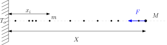
Figure 1: Sketch of the piston model. A gas of particles is confined by a fixed wall (the thermal bath) and a moving wall (the piston) that is subject to a constant external force.

We consider an ideal gas of $N$ pointlike particles with mass $m$, position ${\bf x}_{i}$ and momentum ${\bf p}_{i}$ (${\bf v}_{i}={\bf p}_{i}/m$), $i=1\ldots N$, enclosed in a box. One of the sides of the box is a piston of mass $M$ and momentum $P$ which moves in the $\hat{x}$ direction. Indipendently of the real dimensionality of the box, only the motion in the $\hat{x}$ direction is relevant, as the particles interact only with the piston (see Fig. 1). An externally controlled force $\vec{F}(t)=-F\hat{x}$ acts on the piston. The full (one-dimensional) hamiltonian of the system reads

$$\mathcal{H}=\sum_{i=1}^{N}\frac{p_{i}^{2}}{2m}+\frac{P^{2}}{2M}+FX,$$ (1)

with the additional constraints $0<x_{i}<X$, $i=1,\ldots,N$, and $X>0$. The collisions with the piston are assumed to be elastic

$$V^{\prime} = V+\frac{2m}{m+M}(v_{i}-V),$$

$$v_{i}^{\prime} = v_{i}+\frac{2M}{m+M}(V-v_{i}),$$ (2)

where $v_{i}^{\prime}$ and $V^{\prime}$ are post-collisional velocities. The wall at $x=0$ acts as a thermostat at the temperature $T_{o}$: a collision of a particle with the wall is equivalent to give a new velocity $v^{\prime}$ to the particle with probability density

$$\rho(v^{\prime})=\frac{m}{T_{o}}v^{\prime}e^{-\frac{mv^{\prime 2}}{2T_{o}}}\Theta(v),$$ (3)

where $\Theta(v)$ is the Heaviside Theta. Let us note that the presence of the piston introduces an interaction among the gas particles: for this reason the dynamics of the system depends on the number of particles $N$. As reported in previous studies of systems including the interaction between a piston and one or more gases Lieb (1999); Gruber and Lesne (2006); Cencini et al. (2007); Itami and Sasa (2015), a relevant parameter for the dynamics is $Nm/M$: interesting behaviors are typically observed for values of this parameters $\mathcal{O}(1)$, as in our study. Hereafter we use arbitrary units in numerical simulations, and we put $k_{B}=1$ for the Boltzmann factor. At fixed $F$ and $T_{o}$, the study of the system in the canonical ensemble by means of standard statistical mechanics Cerino et al. (2014); Falcioni et al. (2011) reveals that $\langle X\rangle^{eq}=(N+1)T_{o}/F$ and$\sigma^{2}_{X}=(N+1)T_{o}^{2}/F^{2}$. In addition, if we define the estimate of the instantaneous temperature of the gas,

$$T=\frac{1}{N}\sum_{i=1}^{N}mv_{i}^{2},$$ (4)

the ensemble average of this quantity reads $\langle T\rangle^{eq}=T_{o}$ and its variance is $\sigma^{2}_{T}=2\,T_{o}^{2}/N$.

II.1 The engine protocol

When the parameters $F$ and $T_{o}$ vary in time, mechanical work can be extracted from the system. In particular if we identify the (thermodynamical) internal energy of the system with the value of the hamiltonian, $E(t)=\mathcal{H}({\bf x}(t),t)$, and, in addition, we define the input power as

$$\dot{W}=\left.\frac{\partial\mathcal{H}}{\partial t}\right|_{{\bf x}(t)},$$ (5)

conservation of energy simply reads $\dot{E}(t)=\dot{Q}(t)+\dot{W}(t)$, where $Q$ is the energy absorbed from the thermal wall. For an hamiltonian $\mathcal{H}$ as in Eq. (1) one gets $\dot{W}=X\dot{F}$. Let us remark that this formula is different from the one obtained in standard thermodynamics, $\dot{W}=F\dot{X}$: this is due to the fact that we included the energy of the piston in the internal energy of the system Jarzynski (2007).

Figure 2: Graph of $F$ and $T_{0}$ as a function of time over a cycle period $\tau$.

Here we adopt the following cyclical protocol to obtain a heat engine: the parameters vary periodically in time over a cycle of length $\tau$ (see Fig. 2 and the inset of Fig. 3 for a visual explanation). If we set $t_{0}=k\tau$, with $k$ integer, the cycle has the following form:

1. At times $t\in[t_{0},t_{0}+\tau/4]$: isobaric compression ($F(t)=F_{L}$ and $T_{o}(t)=T_{H}-4(T_{H}-T_{L})(t-t_{0})/\tau$),

2. At times $t\in[t_{0}+\tau/4,t_{0}+\tau/2]$: isothermal compression ($F(t)=F_{L}+4(F_{H}-F_{L})[t-(t_{0}+\tau/4)]/\tau$ and $T_{o}(t)=T_{L}$);

3. At times $t\in[t_{0}+\tau/2,t_{0}+3\tau/4]$ : isobaric expansion ($F(t)=F_{H}$ and $T_{o}(t)=T_{L}+4(T_{H}-T_{L})[t-(t_{0}+\tau/2)]/\tau$);

4. At times $t\in[t_{0}+3\tau/4,t_{0}+\tau]$: isothermal expansion ($F(t)=F_{H}-4(F_{H}-F_{L})[t-(t_{0}+3\tau/4)]/\tau$ and $T_{o}(t)=T_{H}$).

The cycle of length $\tau$ is repeated a large number of times over a long trajectory. In view of a Langevin-like analysis (see below) this protocol (called second type Ericsson cycle) – which is thermostatted for the whole duration of the cycle – is simpler than the more classical Carnot cycle. A similar model has been studied in Izumida and Okuda (2008) with the difference that the velocity of the piston is given and cannot fluctuate (infinite mass $M$ limit). The average values of heat and work in each segment of the cycle can be determined in the adiabatic limit, by substituting at every time $t$ the value of each variable with the equilibrium average: $X(t)=\langle X\rangle^{eq}_{F(t),T_{o}(t)}$ and $E(t)=\langle\mathcal{H}\rangle^{eq}_{F(t),T_{o}(t)}$ (see Table 1).

Segment	$\langle W\rangle$	$\langle Q\rangle$
I)	0	$\frac{3}{2}(N+1)(T_{L}-T_{H})$
II)	$(N+1)T_{L}\ln\left(\frac{F_{H}}{F_{L}}\right)$	$-\langle W\rangle$
III)	0	$\frac{3}{2}(N+1)(T_{H}-T_{L})$
IV)	$-(N+1)T_{H}\ln\left(\frac{F_{H}}{F_{L}}\right)$	$-\langle W\rangle$

Table 1: Table with the adiabatic values of $Q$ and $W$ in each segment of the Ericsson cycle. The average $\langle\cdot\rangle$ is intended over many realization of the cycle.

In particular, let us note that on segments II) and IV) no work is performed and that the heats exchanged have same magnitude but opposite sign. Therefore, in the adiabatic limit, the system does not exchange net heat with any of the intermediate reservoirs at temperature $T_{L}<T^{*}<T_{H}$. Therefore in the rest of the paper we assume that two isobaric transformations do not contribute to the net exchange of heat and work: this is true for $\tau\to\infty$ and seems reasonable, for reasons of symmetry, at large $\tau$, while (small) discrepancies at finite $\tau$ are observed in the simulations. We will denote with $Q_{1}$ the heat exchanged with the cold reservoir $T_{L}$ in sector II), and with $Q_{2}$ the heat exchanged with the thermostat at temperature $T_{H}$ in sector IV). If $\langle Q_{2}\rangle>0$ and $\langle W\rangle<0$, efficiency can be defined as

$$\eta=-\frac{\langle W\rangle}{\langle Q_{2}\rangle},$$ (6)

where $W$ is the total work on a cycle, and $\langle\cdot\rangle$ denotes the average over many realizations of the cycle. Let us remark that this quantity is different from the average over many cycle of the fluctuating efficiency $\hat{\eta}=W/Q_{2}$.

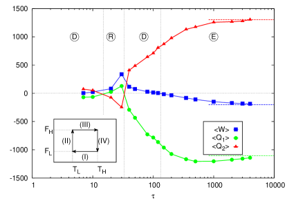
Figure 3: Average values per cycle of work $W$ and heats $Q_{1}$, $Q_{2}$ as a function of the cycle typical time $\tau$. Dashed horizontal lines represent the adiabatic value of such quantities. Inset: schematic of the cycle protocol in the space of parameters $F,T_{o}$.

III Results of MD simulations

In order to perform molecular dynamics simulation of the system with time-dependent parameters $F$ and $T_{o}$, we introduce an interaction potential between the piston and the particles to reproduce the effect of elastic collisions. We choose a repulsive soft sphere potential with cut-off radius $r_{0}$:

$$V(r)=\left[\left(\frac{r_{0}}{r}\right)^{12}+12\frac{r}{r_{0}}-13\right]\Theta(r_{0}-r),$$ (7)

where $\Theta(r)$ is the Heaviside Theta. The parameter $r_{0}$ is to be chosen as small as possible, compatibly with integration time-step $\Delta t$, in order to simulate a contact interaction. In our case $r_{0}=0.2$ and $\Delta t=0.0005$. The values of the other parameters, if not explicitly mentioned, are $m=1$, $M=100$, $N=500$, $T_{L}=11$, $T_{H}=13$, $F_{L}=180$, $F_{H}=220$. The integration scheme adopted is based on the standard Verlet algorithm.

III.1 Average work and heats

In Fig. 3 we report the average values (over $500$ cycles) of $W$, $Q_{1}$ and $Q_{2}$ as a function of $\tau$. In the adiabatic limit, $\tau\gg 10^{3}$, we recover, for $\langle W\rangle$, $\langle Q_{1}\rangle$ and $\langle Q_{2}\rangle$, the values computed assuming quasi-static transformations in thermodynamics. At finite values of the cycle’s duration $\tau<10^{3}$ quite a complex scenario emerges. The absolute value of $\langle W\rangle$ decreases upon reducing $\tau$, until it vanishes at a stall time $\tau^{*}\sim 150$. For shorter cycles, the engine consumes work instead of producing it (the regime at $\tau>\tau^{*}$ is marked, on Fig. 3, as “E”=engine). At smaller $\tau$, the analysis of the heats reveals the existence of three regimes, marked on the Figure as “D”, “R” and again “D”. In the “R” regime the system acts as a refrigerator, i.e. consumes work to push heat from $T_{L}$ to $T_{H}$. In the “D” phases, the heat flow is the standard one (from $T_{H}$ to $T_{L}$), even if work is consumed: however, the rate of heat transfer $\langle Q_{2}\rangle/\tau$ is higher than in the “E” phase, and therefore the machine acts as a more efficient heat sink, similar to dissipating fans. At a time $\tau_{res}<\tau^{*}$ we notice the presence of a maximum in $\langle W\rangle$: it is of the order of magnitude of the adiabatic limit, but with opposite sign. At smaller $\tau\to 0$ the consumed work goes to $0$. Let us note that the relevant timescales emerged from this analysis are in fair agreement with the characteristic relaxation times computed in a simple Langevin model of this system, see below.

III.2 Power and efficiency

Measures of the average developed power $\langle P\rangle=-\langle W\rangle/\tau$ are reported in Fig. 4 (red curve) in the engine phase $\tau>\tau^{*}$. Those measures are given as a function of the efficiency $\eta=-\langle W\rangle/\langle Q_{2}\rangle$, which is monotonically increasing with $\tau$. At a time around $\sim 500$, a maximum is observed in $\langle P\rangle$, whose associated efficiency is found to be slightly smaller than the Curzon-Ahlborn (CA) estimate Curzon and Ahlborn (1975) $\eta_{CA}=1-\sqrt{T_{L}/T_{H}}$. We recall that the CA estimate is based upon an endo-reversible model of Carnot engine where the only entropy changes (even at finite times) occur in the heat transfers. Recently a wider hypothesis for the CA formula has been investigated, which seems to be “symmetric dissipation”, i.e. equal entropy production rates during the two isothermals Esposito et al. (2010). It is likely that our choice of values for $T_{H}$ and $T_{L}=0.85\,T_{H}$ puts us close to that scenario. Nevertheless it is remarkable to recover a result usually derived through macroscopic theories, i.e. without fluctuations, in a small system such as our molecular model.

III.3 Fluctuations

In small systems, fluctuations are hardly negligible Vulpiani et al. (2014). In Fig. 5 (A and B, red curves), we display the behavior of fluctuations of work $W$ integrated in a cycle for two different regimes, at $\tau=50<\tau^{*}$ and $\tau=500>\tau^{*}$. Deviation from a Gaussian behavior are small, indicating that $N$, even if finite, is large enough to expect the validity of the central limit theorem. Interestingly the measure of the standard deviation (stdev) $\sigma_{W}$ rescaled by the average value $\delta W=\sigma_{W}/|\langle W\rangle|$ (black curve in Fig. 5D) shows that $\delta W\ll 1$ close to $\tau_{res}$ and $\delta W\gg 1$ at the stall time $\tau^{*}$. The relative stdev for the heat, $\delta Q_{2}=\sigma_{Q_{2}}/|\langle Q_{2}\rangle|$ behaves much more regularly. It is also interesting to analyze the fluctuation of the “fluctuating efficiency”, i.e. $\hat{\eta}=-W/Q_{2}$ measured in a single cycle, see Fig. 5C (restricted to positive values), which displays a long tail for values larger than the average Verley et al. (2014).

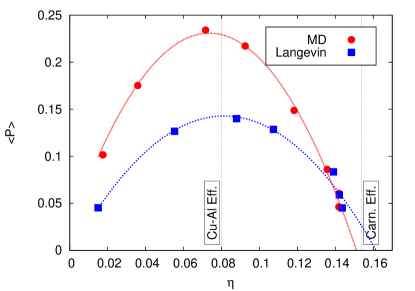
Figure 4: Average power versus efficiency for MD (red curve) and for the reduced “3V” model, Eq. (IV) (blue curve). The Curzon-Ahlborn estimate and the Carnot efficiency are also indicated.

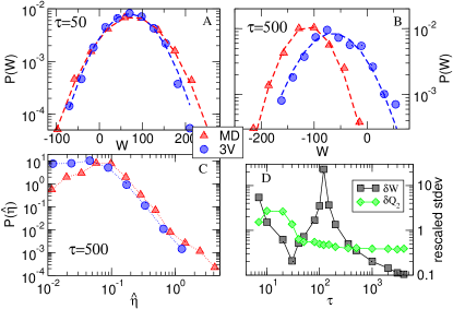
Figure 5: Study of fluctuations. A) and B): Pdf of the work in a cycle for two different values of $\tau$ (“E” and “D” regimes), from the MD and from the reduced “3V” model Eq. (IV). C) Pdf of the fluctuating efficiency in a cycle at $\tau=500$. D) rescaled stdev (see text) of $P(W)$ and of $P(Q_{2})$ as a function of $\tau$. The statistics in this Figure is obtained from $2000$ cycles.

IV Coarse-grained description

In order to make contact with stochastic thermodynamics Seifert (2005), which is a useful framework for small systems, we need a coarse-grained description with few relevant (slowly-changing) variables. The contribution of the fast degrees of freedom is in the noise. Reasonable candidates are: the position of the piston $X$, its velocity $V$ and the estimate of the instantaneous “temperature” of the gas $T(t)=m/N\sum_{i=1}^{N}v_{i}^{2}(t)$. The time evolution of these observables can be determined by computing the average rate of collision occurring between the particles of the gas and the walls of the container. Here, at any $t$, we assume the gas to be homogeneously distributed in the interval $(0,X(t))$ and each particle to have a velocity $v$, given by a Maxwell-Boltzmann distribution $\rho_{T}(v)$ at the temperature $T(t)$. In addition we use the fact that the collisions between the gas particles and the piston are elastic and that a particle that collides with the thermal wall gets a new velocity $v^{\prime}$ distributed according to a Maxwellian distribution $\rho_{o}(v^{\prime})$. Taking into account the contributions of the external force and the collision, we have that the average derivative of the velocity of the piston $\langle\dot{V}\rangle=\lim_{\Delta t\to 0}\langle\Delta V\rangle/\Delta t$ is

$$\langle\dot{V}\rangle=-\frac{F}{M}+\frac{N}{X}\int\,dv\,\,\frac{2m(v-V)^{2}}{(M+m)}\Theta(v-V)\rho_{T}(v).$$ (8)

On the other hand, $\langle\dot{T}(t)\rangle$ is the sum of two terms coming from the collisions with the piston

$$\left.\dot{\langle T\rangle}\right|_{coll}=\frac{m}{X}\int\,dv\,\,(v^{\prime 2}-v^{2})|v-V|\Theta(v-V)\rho_{T}(v),$$ (9)

where $v^{\prime}$ is the velocity after an elastic collision, and the interaction of the gas with the thermostat

$$\left.\dot{\langle T\rangle}\right|_{ther}=\frac{m}{X}\int\,dv\,dv^{\prime}(v^{\prime 2}-v^{2})\,|v|\,\Theta(-v)\,\rho_{T}(v)\rho_{o}(v^{\prime}).$$ (10)

In order to reduce the dynamics to a linear Langevin equation we assume the fluctuations of $X,V$ and $T$ to be small (such assumptions are reasonable if $N\gg 1$ and $M\gg m$) and expand Eqs. (8), (9) and (10) up to the first order around the equilibrium values $X_{eq}=NT_{o}/F$, $V_{eq}=0$ and $T_{eq}=T_{o}$. The linearity of the equation is, on one hand, inspired by the gaussianity of pdfs, and, on the other, it is a useful assumption that allows simple computations. The stochastic part is obtained by adding the gaussian noise terms with amplitudes determined by imposing that the variances of the variables coincide with those computed within the canonical ensemble Cerino et al. (2014). This yields

$$\dot{X} = V,$$

$$\dot{V} = -k(X-X_{eq})-\gamma V+\mu(T-T_{eq})+\sqrt{\frac{2\gamma T_{o}}{M}}\xi_{1},$$

$$\dot{T} = -\frac{2MT_{o}}{N}\mu V-\alpha(T-T_{eq})+\sqrt{\frac{4\alpha T_{o}^{2}}{N}}\xi_{2},$$ (11)

where $\xi_{1}$ and $\xi_{2}$ are independent white noises $\langle\xi_{i}\rangle=0$, $\langle\xi_{i}(t)\xi_{j}(t^{\prime})\rangle=\delta_{ij}\delta(t-t^{\prime})$, ${k(t)=F(t)^{2}/[MNT_{o}(t)]}$, ${\gamma(t)=2F(t)\sqrt{2m/[M^{2}\pi T_{o}(t)]}}$, ${\mu(t)=F(t)/[MT_{o}(t)]}$ and ${\alpha(t)=F(t)\sqrt{2/[mN^{2}\pi T_{o}(t)]}}$. A numerical study of the “3 variables” (3V) model in Eq. (IV) reveals a fair agreement with our main observations. In Fig. 6 the average values per cycle of work and heats are compared with those obtained in the original MD: we define $\dot{W}$ and $\dot{Q}$ as in MD, with $E(t)=NT(t)/2+MV(t)^{2}/2+F(t)X(t)$. The maximum and the inversion of the average work are fully reproduced, but with significant shifts of the values of $\tau$ where they occur. Indeed, a more detailed analysis (not reported here) has identified the relevance of two additional variables: taking into account the position and the velocity of the center of mass of the gas, it is possible to achieve a better agreement with the MD. Unfortunately, the parameters for such a “5 variables” model can only be obtained by fitting the MD data. Notwithstanding its degree of approximation, the $3V$ model gives a fair account of efficiency at maximum power, see Fig. 4, as well as of fluctuations, see Fig. 5A and B, which have a very similar Gaussian shape and width. The overall shape of the efficiency fluctuations’ pdf (Fig. 5C) is also reproduced. The eigenvalues of the dynamic’s matrix in Equations (IV) give also access to typical timescales. For instance, for $F=200$, $T=12$, $M=100$, $m=1$ and $N=500$, the eigenvalues read $\lambda_{1}\approx-0.02$ and $\lambda_{2,3}\approx-0.50\pm i\,\,0.10$ leading to three characteristic timescales to compare with the total duration of the cylce: $\tau_{1}=4/|\lambda_{1}|\approx 170$, $\tau_{2}=4/|\Re(\lambda_{2,3})|\approx 8$ and $\tau_{3}=4/|\Im(\lambda_{2,3})|\approx 40$. Remarkably, the order of magnitude of the relevant timescales in the MD system is correctly reproduced by the eigenvalues of the equilibrium dynamic’s matrix (see Fig. 3 and Fig. 6). A detailed study of the 3V model is out of our present scope, but certainly deserves future investigation.

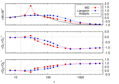
Figure 6: Average work and heats per cycle. Comparison between the MD, the $3$-variables model, Eq. (IV), and the analytical solution in Eq. (V) rescaled by their asymptotic values.

V A solvable toy model

In spite of its apparent simplicity, it is not easy to derive analytical results for the 3V model in a cycle of the external parameters. Here we show that the qualitative dependence of $\langle W\rangle$ on the total time of the cycle $\tau$ can be obtained in a simplified version of Eq. (IV), where we set the temperature $T(t)$ to be equal to the temperature of the thermostat $T_{o}(t)$ at every time $t$. In addition, we assume the parameters to vary in the following form ($\omega=2\pi/\tau$)

$$f(t) = f_{0}(1+\epsilon\cos(\omega t)),$$

$$T(t) = T_{0}(1+q\epsilon\sin(\omega t)),$$ (12)

where ${f(t)=F(t)/M}$, $\epsilon\ll 1$ and ${q\sim\mathcal{O}(1)}$: we set ${f_{0}=2}$, $T_{0}=12$, $\epsilon=0.1$ and $q=0.8$. In the adiabatic limit, this simplified cycle (an approximation of the Ericsson protocol, see Fig. 2) produces a work not very different from the one of the Ericsson cycle. Passing to average values ($Y=\langle X\rangle$) we obtain the equation (see Appendix B):

$$\ddot{Y}+k(t)Y+\gamma(t)\dot{Y}=f(t).$$ (13)

The homogeneous solution associated to Eq. (13) goes to zero in the long time limit: therefore, since we are interested in the asymptotic stationary solution, we will focus only on the non-homogeneous solution. This will be done by expanding all the terms in Eq. (13) in powers of $\epsilon$. In particular, since $Y(t)=Y_{0}(t)+\epsilon Y_{1}(t)+\mathcal{O}(\epsilon^{2})$, by solving Eq. (13) for $\epsilon\to 0$ one gets $Y_{0}(t)=\frac{NT_{0}}{F_{0}}$, and

$$\ddot{Y}_{1}+\omega_{0}^{2}Y_{1}+\nu\dot{Y}_{1}=-f_{0}\cos\omega t+f_{0}q\sin\omega t,$$ (14)

where $\omega_{0}^{2}=F_{0}^{2}/(MNT_{0})$ and $\nu=2f_{0}\sqrt{2m/(\pi T_{0})}$. The asymptotic solution is

$$Y_{1}(t)=A(\omega)[\cos(\omega t+\phi(\omega))-q\sin(\omega t+\phi(\omega))],$$ (15)

$$A(\omega) = \frac{-f_{0}}{\sqrt{\left(\omega_{0}^{2}-\omega^{2}\right)^{2}+\nu^{2}\omega^{2}}},$$

$$\phi(\omega) = \arctan\left(\frac{\nu\omega}{\omega_{0}^{2}-\omega^{2}}\right).$$ (16)

The work performed over a cycle of the parameters of total time $\tau$ can be now expressed in a simple way

$$W(\tau) = -Mf_{0}\frac{2\pi}{\tau}\epsilon\int_{0}^{\tau}dt\,\,(Y_{0}+\epsilon Y_{1}(t))\sin\left(2\pi\frac{t}{\tau}\right)=$$

$$=-Mf_{0}\pi \epsilon^{2} A\left(\frac{2\pi}{\tau}\right)\left[\sin\phi\left(\frac{2\pi}{\tau}\right)-q\cos\phi\left(\frac{2\pi}{\tau}\right)\right].$$ (17)

In Fig. 6 (black curve) it is seen that this result, when normalized to its adiabatic value, compares quite well, in spite of the many approximations introduced to obtain Eq. (V), with the average work performed by the MD system and the 3V model, recovering the change of sign at value not far from $\tau^{*}$ and a maximum at smaller values. Computing the heat transfers is a more difficult task, as it requires a solution of Eq. (13) at order $\mathcal{O}(\epsilon^{2})$.

VI Concluding remarks

Summarizing, we have introduced a new model for a heat engine where fluctuations (due to small $N$) and finite power (due to small $\tau$) are observed. In the past a great attention has been given to extremely simplified models, typically in the form of single molecules or colloids, or Markov chains inspired to biochemical reactions. Here we propose to move towards a higher level of complexity, and possibly realism, suggesting a new test-ground for statistical mechanics of small systems out-of-equilibrium. Our system reveals non-trivial features, such as several working regimes (engine, refrigerator, heat sink) tuned by simply controlling $\tau$. Notwithstanding its rich phenomenology, the model admits a coarse-grained description in terms of three linearly coupled Langevin equations. Further investigation of this reduced model are in order, in particular of heat, work and efficiency fluctuations Verley et al. (2014).

Appendix A Details on the derivation of the Langevin Equation

In order to get a linear Langevin equation from kinetic theory we start from the conditional equilibrium distribution with fixed values of the macroscopic variables $X,V,T$, and then determine the average number of particles that, in the unit time $\Delta t$, collide with the piston or with the thermal wall. Using Eq. (II) and (3), one can determine post-collisional velocities and, accordingly, the average change of $V$ and $T$, over a time $\Delta t$. In the following, to simplify the notation, we denote with $\langle\cdot\rangle$ the conditional average $\langle\cdot|X,V,T\rangle$.

The equation for $X$ reads $\dot{X}=V$. The total average force acting on the piston due to collisions is:

$$\lim_{\Delta\to 0}\frac{\langle\Delta V\rangle_{coll}}{\Delta t}=$$ (18)

$$= \frac{N}{X}\int_{0}^{\infty}dv\,\frac{2m}{m+M}(v-V)|V-v|\rho_{T}(v)\Theta(V-v)=$$

$$= \frac{2Nm}{(M+m)X}\sqrt{\frac{m}{2\pi T}}\int_{V}^{\infty}dv\,\,(v-V)^{2}e^{-m\frac{v^{2}}{2T}}=$$

$$= \frac{N}{(m+M)X}\Bigg{(}\left(T+mV^{2}\right)\text{erfc}\left(\sqrt{\frac{m}{2T}}V\right)+$$

$$-\leavevmode\nobreak\ \leavevmode\nobreak\ \sqrt{\frac{2mTV^{2}}{\pi}}e^{-\frac{mV^{2}}{2T}}\Bigg{)},$$

where $\text{erfc}(x)=2/\sqrt{\pi}\int_{x}^{\infty}dt\exp(-t^{2})$. To obtain the total force, a term $-F/M$ must be added. The elastic collisions with the piston also affect the kinetic energy of the gas, through the term

$$\left.\dot{\langle T\rangle}\right|_{coll} = \frac{m}{X}\int\,dv\,\,(v^{\prime 2}-v^{2})|v-V|\Theta(v-V)\rho_{T}(v)=$$ (19)

$$= \frac{m}{X}\sqrt{\frac{m}{2\pi T}}\int_{V}^{\infty}dv\,\left[\left(v+2\frac{M}{m+M}(V-v)\right)^{2}-v^{2}\right](v-V)e^{-m\frac{v^{2}}{2T}}=$$

$$= -\frac{2M}{(m+M)^{2}X}\left(\sqrt{\frac{2mT}{\pi}}\left(2T-MV^{2}\right)e^{-\frac{mV^{2}}{2T}}+V\left(MT+mMV^{2}-2mT\right)\text{erfc}\left(\sqrt{\frac{m}{2T}}V\right)\right).$$

Finally, the average change of temperature in a time interval $\Delta t$, due to the collision with the thermal wall is simply given by the term

$$\left.\dot{\langle T\rangle}\right|_{ther} = \frac{m}{X}\int\,dv\,dv^{\prime}(v^{\prime 2}-v^{2})\,|v|\,\Theta(-v)\,\rho_{T}(v)\rho_{o}(v^{\prime})=$$ (20)

$$= -\frac{m^{2}}{XT_{o}}\sqrt{\frac{m}{2\pi T}}\int_{-\infty}^{0}dv\int_{0}^{\infty}dv^{\prime}\,\,\left(v^{\prime 2}-v^{2}\right)vv^{\prime}e^{-m\frac{v^{2}}{2T}}e^{-m\frac{v^{\prime 2}}{2T_{o}}}=$$

$$= \sqrt{\frac{2}{\pi m}}\frac{\sqrt{T}(T_{o}-T)}{X}.$$

The equilibrium value of $X,V$ and $T$ for which $\langle\dot{X}\rangle=0$, $\langle\dot{V}\rangle=0$ and $\dot{T}=\left.\dot{\langle T\rangle}\right|_{coll}+\left.\dot{\langle T\rangle}\right|_{ther}=0$ are

$$X_{eq} = N\frac{T_{o}}{F},$$ (21)

$$V_{eq} = 0,$$ (22)

$$T_{eq} = T_{o},$$ (23)

where terms $\mathcal{O}(m/M)$ are neglected. We can obtain a linear equation by expanding the expressions above up to first order around the equilibrium values: this can be done only if fluctuations are small, i.e. when $N\gg 1$ and $M\gg m$. The sum of Eq. (18) and $-F/M$ yelds

$$\langle\dot{V}\rangle=-k(X-X_{eq})-\gamma V+\mu(T-T_{eq}),$$ (24)

with $k=F^{2}/MNT_{o}$, $\gamma=2F\sqrt{2m/(M^{2}\pi T_{o})}$ and $\mu=F/(MT_{o})$ . Similarly the sum of Eq. (19) and Eq. (20) yelds

$$\langle\dot{T}\rangle=-\frac{2MT_{o}}{N}\mu V-\alpha(T-T_{eq}),$$ (25)

with $\alpha=F\sqrt{2/(mN^{2}\pi T_{o})}$. The coefficients $k,\gamma,\mu$ and $\alpha$ vary in time according to the time evolution of $F$ and $T_{o}$. In order to take into account the fluctuations of this variables one must add three independent gaussian terms $\xi_{X}\equiv\xi_{0}$, $\xi_{V}\equiv\xi_{1}$ and $\xi_{T}\equiv\xi_{2}$, with an appropriate weight matrix $b_{ij}$ with $i,j=0,1,2$. In this particular case the matrix is diagonal, $b_{ii}=b_{i}$, with $b_{0}=0$, $b_{1}=\sqrt{2\gamma\sigma^{2}_{V}}$ and $b_{2}=\sqrt{2\gamma\sigma^{2}_{T}}$. The final form of the linear Langevin equation thus reads

$$\dot{X} = V,$$

$$\dot{V} = -k(X-X_{eq})-\gamma V+\mu(T-T_{eq})+\sqrt{\frac{2\gamma T_{o}}{M}}\xi_{1},$$

$$\dot{T} = -\frac{2MT_{o}}{N}\mu V-\alpha(T-T_{eq})+\sqrt{\frac{4\alpha T_{o}^{2}}{N}}\xi_{2}.$$ (26)

Let us note that this equation, with fixed $F$ and $T_{o}$, satisfies detailed balance Gardiner (1985).

Appendix B Details on the analytic solution of the toy model

Let us consider Eq. (13):

$$\ddot{Y}+k(t)Y+\gamma(t)\dot{Y}=f(t),$$ (27)

where

$$\gamma(t) = \frac{2F(t)}{M}\sqrt{\frac{2m}{\pi T_{o}(t)}},$$

$$k(t) = \frac{F(t)^{2}}{MNT_{o}(t)},$$ (28)

and $f(t)=F(t)/M$. In the Ericsson cycle $F$ and $T$ depend on time in a too complicated manner in order to perform analytic calculations. Therefore, in order to obtain an explicit result, in the following we will assume

$$f(t) = f_{0}(1+\epsilon\cos(\omega t)),$$

$$T_{o}(t) = T_{0}(1+q\epsilon\sin(\omega t)),$$ (29)

where $\omega=2\pi/\tau$, $\epsilon\ll 1$ and $q\sim\mathcal{O}(1)$. We will now sketch the derivation of the non-homogeneous solution of Eq. (27) as an asymptotic expansion in $\epsilon\ll 1$. Let us expand in power of $\epsilon$ all the coefficients appearing in Eq. (27) up to $\mathcal{O}(\epsilon)$

$$k(t) \approx \frac{Mf_{0}^{2}}{NT_{0}}\left[1+(2\cos\omega t-q\sin\omega t)\epsilon\right]$$ (30)

$$\gamma(t) \approx \sqrt{\frac{4f_{o}^{2}m}{\pi T_{0}}}\left[1+\left(\cos\omega t-\frac{q}{2}\sin\ \omega t\right)\epsilon\right]$$

$$Y(t) \approx Y_{0}(t)+\epsilon Y_{1}(t).$$ (31)

Plugging these expressions into Eq. (27), for $\epsilon=0$ one gets

$$\ddot{Y}_{0}+\frac{Mf_{0}^{2}}{NT_{0}}Y_{0}+2f_{0}\sqrt{\frac{2m}{\pi T_{0}}}\dot{Y}_{0}=f_{0},$$ (32)

leading to

$$Y_{0}(t)=\frac{NT_{0}}{F_{0}}.$$ (33)

At the following order $\mathcal{O}(\epsilon)$, Eq. (27) gives

$$\ddot{Y}_{1}+\frac{Mf_{0}^{2}}{NT_{0}}(Y_{1}+(2\cos\omega t-q\sin\omega t)Y_{0})+$$

$$2f_{0}\sqrt{\frac{2m}{\pi T_{0}}}\left(\dot{Y}_{1}+\left(\cos\omega t-\frac{q}{2}\sin\ \omega t\right)\dot{Y}_{0}\right)=$$

$$=f_{0}\cos\omega t$$ (34)

or, if we plug the value of $Y_{0}$,

$$\ddot{Y}_{1}+\omega_{0}^{2}Y_{1}+\nu\dot{Y}_{1}=-f_{0}\cos\omega t+f_{0}q\sin\omega t,$$ (35)

where $\omega_{0}=\sqrt{Mf_{0}^{2}/(NT_{0})}$ and $\nu=2f_{0}\sqrt{2m/(\pi T_{0})}$. A solution of this equation can be found in the form

$$Y_{1}(t)=A(\omega)(\cos(\omega t+\phi(\omega))+q\sin(\omega t+\phi(\omega))),$$ (36)

where

$$A(\omega) = \frac{-f_{0}}{\sqrt{\left(\omega_{0}^{2}-\omega^{2}\right)^{2}+\nu^{2}\omega^{2}}},$$ (37)

$$\phi(\omega) = \arctan\left(\frac{\nu\omega}{\omega_{0}^{2}-\omega^{2}}\right).$$ (38)

References

- Castiglione et al. (2008) P. Castiglione, M. Falcioni, A. Lesne, and A. Vulpiani, Chaos and coarse graining in statistical mechanics (Cambridge University Press, 2008).
- Reichl (2009) L. Reichl, A Modern Course in Statistical Physics (Wiley-VCH, 2009).
- Gaspard (2006) P. Gaspard, Phys. A: Math. Gen. 369, 201 (2006).
- Andresen et al. (1977) B. Andresen, R. Berry, A. Nitzan, and P. Salamon, Physical Review A 15, 2086 (1977).
- Van den Broeck (2005) C. Van den Broeck, Physical Review Letters 95, 190602 (2005).
- Bustamante et al. (2005) C. Bustamante, J. Liphardt, and F. Ritort, Physics Today 58, 43 (2005).
- Marconi et al. (2008) U. M. B. Marconi, A. Puglisi, L. Rondoni, and A. Vulpiani, Physics Reports 461, 111 (2008).
- van Kampen (2007) N. G. van Kampen, Stochastic Processes in Physics and Chemistry (Elsevier, 2007).
- Sekimoto (2010) K. Sekimoto, Stochastic energetics (Springer Verlag, 2010).
- Seifert (2011) U. Seifert, Physical Review Letters 106, 020601 (2011).
- Sato et al. (2002) K. Sato, K. Sekimoto, T. Hondou, and F. Takagi, Phys. Rev. E 66, 016119 (2002).
- Sano and Hayakawa (2014) T. G. Sano and H. Hayakawa, (2014), arxiv:1412.4468.
- Itami and Sasa (2015) M. Itami and S. Sasa, J. Stat. Phys. 158, 37 (2015).
- Lieb (1999) E. H. Lieb, Physica A 263, 491 (1999).
- Gruber and Lesne (2006) C. Gruber and A. Lesne, in Encyclopedia of Mathematical Physics (Elsevier Amsterdam, 2006).
- Cencini et al. (2007) M. Cencini, L. Palatella, S. Pigolotti, and A. Vulpiani, Phys. Rev. E 76, 051103 (2007).
- Cerino et al. (2014) L. Cerino, G. Gradenigo, A. Sarracino, D. Villamaina, and A. Vulpiani, Physical Review E 89, 42105 (2014).
- Falcioni et al. (2011) M. Falcioni, D. Villamaina, A. Vulpiani, A. Puglisi, and A. Sarracino, American Journal of Physics 79, 777 (2011).
- Jarzynski (2007) C. Jarzynski, C. R. Physique 8, 495 (2007).
- Izumida and Okuda (2008) Y. Izumida and K. Okuda, Europhys. Lett. 83, 60003 (2008).
- Curzon and Ahlborn (1975) F. Curzon and B. Ahlborn, American Journal of Physics 43, 22 (1975).
- Esposito et al. (2010) M. Esposito, R. Kawai, K. Lindenberg, and C. Van den Broeck, Physical Review Letters 105, 150603 (2010).
- Vulpiani et al. (2014) A. Vulpiani, F. Cecconi, M. Cencini, A. Puglisi, and D. Vergni, eds., Large Deviations in Physics (Springer, 2014).
- Verley et al. (2014) G. Verley, M. Esposito, T. Willaert, and C. Van den Broeck, Nature Communications 5, 4721 (2014).
- Seifert (2005) U. Seifert, Physical Review Letters 95, 040602 (2005).
- Gardiner (1985) C. W. Gardiner, Handbook of stochastic methods (Springer Berlin, 1985).