Quantum Monte Carlo estimation of complex-time correlations for the study of the ground-state dynamic structure function

Abstract

We present a method based on the Path Integral Monte Carlo formalism for the calculation of ground-state time correlation functions in quantum systems. The key point of the method is the consideration of time as a complex variable whose phase $\delta$ acts as an adjustable parameter. By using high-order approximations for the quantum propagator, it is possible to obtain Monte Carlo data all the way from purely imaginary time to $\delta$ values near the limit of real time. As a consequence, it is possible to infer accurately the spectral functions using simple inversion algorithms. We test this approach in the calculation of the dynamic structure function $S(q,\omega)$ of two one-dimensional model systems, harmonic and quartic oscillators, for which $S(q,\omega)$ can be exactly calculated. We notice a clear improvement in the calculation of the dynamic response with respect to the common approach based on the inverse Laplace transform of the imaginary-time correlation function.

Keywords: quantum Monte Carlo, inverse problem, dynamic structure

I Introduction

In the last decades, quantum Monte Carlo (QMC) methods have been extensively used in the field of quantum many-body physics. Many of these numerical techniques rely on stochastic propagation in imaginary time and can provide extremely accurate results for the thermodynamic and static properties of many-body systems, even in those where quantum correlations make unavoidable the use of non-perturbative approaches.CeperleyRMP ; Sarsa00 ; electrongas ; unitary The main drawback of QMC methods is the difficulty arising in the calculation of spectral functions. These functions, which are particularly relevant for the study of the dynamical properties of quantum many-body systems (e.g. the excitation spectrum or the transport coefficients), can be obtained as Fourier transforms of real-time correlation functions. A QMC calculation of these quantities, however, is particularly inefficient since the rapidly oscillating exponentials appearing in the definition of real-time propagators make the statistical errors grow exponentially with time. Many approximation schemes have been developed and used to investigate the dynamic properties of quantum many-body systems. For instance, centroid cao or ring-polymer molecular dynamicscraig has been successfully applied to the study of quantum many-body systems in the semi-classical regime. In the limit of zero temperature, an alternative approach is to use correlated perturbation theorykrotscheck relying on the ground-state properties of the system obtained with QMC calculations. mazzanti ; Macia12 ; krotscheck2

Nevertheless, the mainstream approaches to the calculation of spectral functions from QMC simulations consist in attempting a numerical inversion of a Laplace transform. This integral transform relates the desired spectral functions to the correlation functions in imaginary time, easily attainable with QMC methods. However, the inverse Laplace transform of noisy data is an ill-posed problem. This means that, given a particular set of data for the imaginary-time correlation function, it is hardly possible to recover a unique, well-defined solution to the problem. Sophisticated regularization techniques can then be used to reproduce a reasonable estimate of the spectral function. InvProbTextbook In the last decades, several algorithms to deal with the inverse Laplace transform of noisy data have been proposed, Jarrell96 ; Boninsegni96 ; Sandwik98 ; Mishchenko00 ; Vitali10 but these methods can only be reliably applied to the analysis of the low-energy dynamic properties of quantum systems, since the Laplace kernel tends to suppress high-energy contributions. In order to overcome these limitations and to get more accurate results of spectral functions from QMC data, it is necessary to develop new estimators for the quantum time correlation functions.  Roggero13

In this work, we propose to infer the dynamic structure function of a quantum system at zero temperature from a QMC estimation of the corresponding correlation function in complex time. Similar approaches have been already used for studying the dynamic properties of quantum systems at finite temperature $T$. In this case, the $e^{-\beta\hat{H}}$ term (with $\beta=1/T$) appearing in the definition of the thermal averages can be considered as an evolution operator in imaginary time. Thus, the real-time correlation function can be rewritten in terms of a correlation function in complex time, Schofield ; Thirumalai84 which can be calculated using path-integral formalismFeynman and estimated in QMC calculations.Chakrabarti98 Even though this estimation is reliable only for times $t\lesssim\hbar\beta$, the spectral functions obtained within this approach exhibit a significant improvement over the results derived from analytic continuation of imaginary-time correlation functions. Krilov01 ; Sim01 ; Krilov01CP ; Nakayama06 ; Kegerreis08 ; Jadhao08 ; Bonella10a ; Bonella10b

Our goal is to extend this formalism to the calculation of ground-state time correlation functions, even considering that at zero temperature the notion of complex time has not a precise physical meaning. This strategy allows us to introduce an adjustable parameter, namely the phase $\delta$ of the complex time $t_{c}=|t_{c}|e^{-i\delta}$, which makes possible to calculate the correlation function in an intermediate regime between the commonly used imaginary time ($\delta=\pi/2$) and real time ($\delta=0$).

More precisely, we sample paths connecting two configurations distributed according to the ground-state wave function of the quantum system and calculate, over these paths, the propagator at the complex time $t_{c}$. Changing the phase $\delta$, we can find an optimal value for which the correlation functions estimated with QMC are affected by moderate statistical errors and, at the same time, present a relevant amount of information on the real dynamics of the quantum system. This approach makes it possible to infer the spectral functions using rather simple inversion techniques since the ill-posed character of the inversion procedure is appreciably reduced. In this way, more accurate and more stable results than the usual ones, based on the inverse Laplace transform of imaginary-time data, can be obtained.

Similarly to what happens in the case at finite temperature, the QMC estimation of the ground state correlation function in complex time is reliable only up to a certain value of $|t_{c}|$ depending on $\delta$, above which the statistical error becomes too large and makes the numerical results meaningless. It is therefore crucial to develop strategies that make the range of accessible times as large as possible. In this work, we propose to tackle this problem using high-order approximations for the quantum propagator. chin In particular, we show that the propagator derived by Zillich et al. Zillich10 is particularly suitable for the complex-time evolution.

The rest of the paper is organized as follows. In Sec. II, we discuss the QMC method that we have devised for the calculation of complex-time correlation functions and, more briefly, the inversion method that we have used to obtain the dynamic structure function. In Sec. III, the results obtained with this method in one-dimensional problems are shown and compared with the standard approach relying only on imaginary-time correlation functions. Finally, the summary and main conclusions are reported in Sec. IV.

II Method

II.1 Calculation of the complex-time correlation function

The main objective of our work is the calculation of ground-state time correlation functions of a quantum system. At zero temperature, a general time correlation function is defined as

$$C_{AB}(t_{c})=\langle\Psi_{0}|e^{it_{c}\hat{H}/\hbar}\hat{A}e^{-it_{c}\hat{H}/\hbar}\hat{B}|\Psi_{0}\rangle\ ,$$ (1)

where $\hat{A}$ and $\hat{B}$ are time-independent quantum mechanical operators in the Schrödinger picture corresponding to measurable observables, $\hat{H}$ is the Hamiltonian, and $|\Psi_{0}\rangle$ is the ground state. For the sake of simplicity, in the following we consider correlations among operators which are diagonal in coordinate space and use one-dimensional notation (the generalization to multi-dimensional space is straightforward).

The main idea of this work is to calculate $C_{AB}(t_{c})$, defined in Eq. 1, where $t_{c}$ has been analytically extended to the complex plane. We indicate with $t_{m}>0$ and $-\delta$ the modulus and the phase of the complex time, $t_{c}=t_{m}e^{-i\delta}$, respectively. In order to elaborate a form for the estimator of $C_{AB}(t_{c})$ implementable in computer simulations, we rewrite Eq. 1 in the coordinate space,

$$C_{AB}(t_{c}) = \int dx_{0}dx_{M}\,e^{it_{c}E_{0}}\langle\Psi_{0}|x_{M}\rangle\langle x_{M}|\hat{A}e^{-it_{c}\hat{H}}\hat{B}|x_{0}\rangle\langle x_{0}|\Psi_{0}\rangle\ =$$ (2)

$$= \mathcal{N}\int dx_{0}dx_{M}\,\Psi_{0}^{\star}(x_{M})A(x_{M})G(x_{0},x_{M};t_{c})B(x_{0})\Psi_{0}(x_{0})\ ,$$

where $G(x_{0},x_{M};t_{c})=\langle x_{M}|e^{-it_{c}\hat{H}}|x_{0}\rangle$ is the propagator from position $x_{0}$ to position $x_{M}$ in complex time $t_{c}$, and $\mathcal{N}$ is a normalization constant. In the general case of complex time $t_{c}$, the propagator $G(x_{0},x_{M};t_{c})$ is a complex function that becomes real and positive only when $t_{c}$ is a purely imaginary time. Thus, the function $G(x_{0},x_{M};t_{c})$ cannot be used as a probability distribution function for the sampling of coordinates in any QMC algorithm (as it is normally done, for instance, in the PIMC method). Therefore, what we do is to sample first the positions $x_{0}$ and $x_{M}$ according to a probability distribution constructed from an accurate approximation to the ground-state wave function. This sampling can be performed using any conventional QMC technique at zero temperature. In this work, we use the Path Integral Ground State (PIGS) method. Sarsa00 ; Rota10 Then, having sampled the positions $x_{0}$ and $x_{M}$, we calculate $C_{AB}(t_{c})$ estimating the quantity $A(x_{M})G(x_{0},x_{M};t_{c})B(x_{0})$.

In order to carry on this procedure one needs to know the exact form of the Green’s function $G(x_{0},x_{M};t_{c})$ for any value $t_{c}$, but this is in general unknown. However, what is possible is to construct accurate approximations to the propagator in the limit of small $t_{m}=|t_{c}|$. Then, to estimate $C_{AB}(t_{c})$ for larger values of $t_{m}$ we use the path-integral formalism to rewrite $G(x_{0},x_{M};t_{c})$ as a convolution of $M$ propagators of a shorter time $\varepsilon_{c}=t_{c}/M$,

$$G(x_{0},x_{M};t_{c})=\int dx_{1}\ldots dx_{M-1}\prod_{k=1}^{M}G\left(x_{k},x_{k-1};\varepsilon_{c}\right)\ .$$ (3)

Within this approach, it becomes necessary to sample all the configurations $\{x_{1},x_{2},\ldots,x_{M-1}\}$, i.e., to build paths from the position $x_{0}$ to the position $x_{M}$. However, the choice of the probability distribution $p_{\text{path}}(x_{0},x_{1},\ldots,x_{M})$ for these paths is not trivial and depends on the system studied. Generally, we notice that using imaginary-time propagator to this end is not a good choice, because in this case the sampled paths would remain close to the minimum energy path and the estimator would not be able to capture all the contributions to $C_{AB}$ coming from the excited states. As a simple and flexible enough option, it is possible to choose $p_{\text{path}}$ as the product of $M$ free propagators of imaginary-time step $\tau_{s}$,

$$p_{\text{path}}(x_{0},x_{1},\ldots,x_{M})=\prod_{k=1}^{M}G_{\text{free}}(x_{k},x_{k-1};\tau_{s})\ ,$$ (4)

with

$$G_{\text{free}}(x_{k},x_{k-1};\tau_{s})=(4\pi\lambda\tau_{s})^{Nd/2}\exp\left(-\frac{(x_{k}-x_{k-1})^{2}}{4\lambda\tau_{s}}\right)\ .$$ (5)

In Eq. 5, $N$ is the number of particles, $d$ is the dimensionality of the system, and $\lambda=\hbar^{2}/(2m)$. This choice indeed allows to construct the paths by means of simple sampling techniques which do not require a large computational effort, like for instance the staging algorithm. stag1 ; stag2 In the case of quantum systems interacting with a smooth potential, we notice that it is possible to obtain good results for $C_{AB}(t_{c})$ using $p_{\text{path}}$ in Eq. 4, provided that the parameter $\tau_{s}$ is properly chosen. Indeed, we see that the variance of the estimator for $C_{AB}(t_{c})$ is reduced when the free propagator in the imaginary time $\tau_{s}$ is similar to the modulus of the kinetic propagator in the complex time $\varepsilon_{c}$.

Since the purpose of this work is to test our QMC approach in two model systems interacting with smooth potentials (the quantum harmonic and quartic oscillators), we decide to use this choice of $p_{\text{path}}$ with $\tau_{s}\simeq(\Re[1/(i\varepsilon_{c})])^{-1}$ to perform the sampling of the paths $\{x_{1},x_{2},\ldots,x_{M-1}\}$. Nevertheless, this may not be the best choice in general, and one may have to use more sophisticated and more computationally demanding algorithms for the sampling of the paths.

Once the probability distribution $p_{\text{path}}$ is chosen, the expression of the ground state complex time correlation function becomes

$$C_{AB}(t_{c}) = \mathcal{N^{\prime}}\int dx_{0}\ldots dx_{M}A(x_{M})\frac{\prod_{k=1}^{M}G(x_{k},x_{k-1};\varepsilon_{c})}{p_{\text{path}}(x_{0},x_{1},\ldots,x_{M})}B(x_{0})\times$$ (6)

$$\Psi_{0}(x_{M})p_{\text{path}}(x_{0},x_{1},\ldots,x_{M})\Psi_{0}(x_{0})\ .$$

At this point, one has to choose an approximation scheme for $G(x_{k},x_{k-1};\varepsilon_{c})$ in order to derive an analytical expression that can be implemented in computer simulations. Increasing the number of convolution terms $M$, and thus decreasing the modulus of $\varepsilon_{c}$, it is possible to systematically improve the quality of the approximation and to asymptotically recover the exact correlation function. Nevertheless, every propagator $G(x_{k},x_{k-1};\varepsilon_{c})$ introduces an oscillating phase term in the integrand of Eq. 6, and thus the statistical noise of the estimator for $C_{AB}(t_{c})$ increases notably when $M$ becomes large. In order to obtain reliable results, it is fundamental to develop numerical strategies that keep the number $M$ of convolution terms as low as possible.

The simplest approximation to the propagator is the primitive approximation (PA), which relies on the factorization $e^{it_{c}\hat{H}}\simeq e^{it_{c}\hat{K}}e^{it_{c}\hat{V}}$, where $\hat{K}$ and $\hat{V}$ are the kinetic and potential operators, respectively. In this scheme, the complex-time propagator can be written as

$$G(x_{k},x_{k-1};\varepsilon_{c}) \simeq G_{PA}(x_{k},x_{k-1};\varepsilon_{c})=$$ (7)

$$= \exp\left(-\frac{(x_{k}-x_{k-1})^{2}}{4\lambda\,i\varepsilon_{c}}\right)\exp\left(-i\frac{V(x_{k})+V(x_{k-1})}{2\hbar}\varepsilon_{c}\right)\ .$$

The PA approximation is easily implementable within our QMC procedure but requires a large number $M$ of convolution terms in Eq. 6. In order to improve the accuracy, it is important to use higher-order approximations to the complex-time propagator. In conventional PIMC simulations, a significant improvement in efficiency can be obtained using symplectic expansions of the time-evolution operator that incorporates double commutators between kinetic and potential operators. TakahashiImada ; chin For local potentials, these commutators lead to extra terms that are exponentials of the gradient of the potential squared times the third power of the time step. The inclusion of this contribution in the propagator largely improves the efficiency of the PIMC Sakkos09 and PIGS Rota10 methods. In imaginary-time propagation, the contribution of the double commutator always appears in the argument of the exponential with a negative sign. However, in complex time this sign turns out to be positive for $\delta<60^{0}$, producing largely increasing amplitudes and thus unreliable results that make the use of this high-order scheme unpractical (see Appendix A). Therefore, it is very important to look for other expansions which can improve the PA but that do not include double-commutator terms.

A high-order approximation for the complex-time propagator without double commutator has been reported in Ref. Zillich10, . In that work, the authors were able to improve the quality of the small-time propagator by introducing a linear combination, with some negative coefficients, of different symplectic expansions on the same time. This expansion has some drawbacks when used in conventional PIMC simulations, since it gives rise to an approximation for the imaginary-time propagator which is not positive definite. This feature does not represent a problem here, since in the calculation of $C_{AB}(t_{c})$ the complex-time propagator is not used as the probability distribution of the Monte Carlo sampling but rather as the estimator.

Once we have chosen the approximation for the complex-time propagator, the only thing that is still lacking in order to calculate $C_{AB}(t_{c})$ is the normalization constant $\mathcal{N^{\prime}}$. This can be computed imposing the autocorrelation function of the identity operator to be $1$ for any value of $t_{c}$. Therefore, if we define the complex quantity

$$O_{A}(x_{0},\ldots,x_{M})=\frac{\prod_{k=1}^{M}G_{A}(x_{k},x_{k-1};\varepsilon_{c})}{p_{\text{path}}(x_{0},x_{1},\ldots,x_{M})}\ ,$$ (8)

where $G_{A}(x_{k},x_{k-1};\varepsilon_{c})$ is the chosen approximation for the time propagator, the complex-time correlation function in Eq. 6 can be written as

$$C_{AB}(t_{c})=\frac{\langle A(x_{M})O_{A}(x_{0},\ldots,x_{M})B(x_{0})\rangle}{\langle O_{A}(x_{0},\ldots,x_{M})\rangle}\ .$$ (9)

The bracket $\langle\ldots\rangle$ indicates the averages over the configurations $\{x_{0},x_{1},\ldots,x_{M}\}$ sampled following the scheme described above, i.e., with $x_{0}$ and $x_{M}$ sampled according to a reasonable approximation of the ground-state wave function, and $\{x_{1},x_{2},\ldots,x_{M-1}\}$ sampled according to the probability distribution $p_{\text{path}}(x_{0},x_{1},\ldots,x_{M})$.

Summarizing, the evaluation of $C_{AB}(t_{c})$ (9) for a given complex time $t_{c}=t_{m}e^{-i\delta}$ consists of the following steps:

1. To generate the $x_{0}$ and $x_{M}$ configurations according to the probability distribution $\Psi_{0}(x_{0})\Psi_{0}(x_{M})$, by means of a QMC technique at zero temperature, like the PIGS algorithm.

2. To choose $M$ (number of points of the discrete path from $x_{0}$ to $x_{M}$), so that the parameter $\varepsilon_{m}=t_{m}/M$ is sufficiently small to recover the $\varepsilon_{m}\to 0$ limit. In practice, one selects the value of $M$ that makes $\varepsilon_{m}=t_{m}/M<\varepsilon_{m}^{*}$, where the parameter $\varepsilon_{m}^{*}$ depends on the accuracy of the approximated action.

3. To generate the configurations $\{x_{1},x_{2},\ldots,x_{M-1}\}$, i.e., the path from $x_{0}$ to $x_{M}$, according to the probability distribution $p_{\text{path}}$.

4. To evaluate $O_{A}(x_{0},\ldots,x_{M})$ from Eq. 8 and accumulate the estimator of $C_{AB}(t_{c})$ defined in Eq. 9.

II.2 Inversion technique

Once we have obtained the QMC data for the complex-time correlation function $C_{AB}(t_{c})$, we need to recover the desired spectral function $S_{AB}(\omega)$ inverting the integral transform

$$C_{AB}(t_{c})=\int d\omega\,e^{-it_{c}\omega}S_{AB}(\omega)\ .$$ (10)

Considering that both the function $C_{AB}(t_{c})$ and $S_{AB}(\omega)$ are evaluated over a finite set of complex times $\{t_{c\,i}\}$ and frequencies $\{\omega_{j}\}$, Eq. 10 is formally equivalent to a linear equation

$$y=A\,x\ ,$$ (11)

where the vector $y$ represents the QMC data for the correlation function $C_{AB}(t_{c})$, the vector $x$ the spectral function $S_{AB}(\omega)$ that we want to obtain, and $A$ is a matrix defined from the kernel of the integral transform (10) which relates $C_{AB}(t_{c})$ and $S_{AB}(\omega)$. Notice that $C_{AB}(t_{c})$ is a complex function: thus, its real and its imaginary part provide two different rows of the matrix $A$, both of them real.

The best least-squares solution to Eq. 11 is given by the pseudo-inverse matrix

$$x=A^{T}(A\,A^{T})^{-1}\,y\ .$$ (12)

In well-posed problems, Eq. 12 directly provides useful solutions. If $x$ has larger dimensionality than $y$, then the linear equation in (11) has an infinite number of solutions, and (12) provides the one which minimizes $|x|^{2}$. Contrarily, if $x$ has lower dimensionality than $y$, then no solution exists and Eq. 12 (using the Moore-Penrose pseudoinverse if $AA^{T}$ is not full-rank) provides the $x$ vector which minimizes $|y-Ax|^{2}$, i.e., a best fit to the $y$ data is obtained.

However, when the eigenvalues of the matrix $AA^{T}$, which are all positive or zero, span a range of many orders of magnitude (in the numerical inversions performed in the present work, eigenvalues of $AA^{T}$ covering the range $10^{0}$-$10^{-20}$ are routinely found), the inversion problem becomes ill-posed, and the solution $x$ to Eq. 12 is extremely sensitive to errors in the vector $y$. The ill-posed nature of the inversion process means that the statistical noise in the original data for $C_{AB}(t_{c})$, that is unavoidable in any QMC calculation, is uncontrollably magnified in the inversion process, resulting in a meaningless solution for the spectral function $S_{AB}(\omega)$.

In these situations, regularization techniques are useful to obtain meaningful solutions to the ill-posed problem. key-1 The basic idea of these methods is to define a well-conditioned linear operator $C_{a}$ which depends on a regularization parameter $a>0$ that approaches the pseudo-inverse $A^{+}=A^{T}(AA^{T})^{-1}$ in the limit $a\to 0$. Then, the solution of the original problem can be obtained as $x=\lim_{a\to 0}C_{a}y$.

In this work, we have chosen to use the Tikhonov regularization, key-2 in which

$$C_{a}=A^{T}(A\,A^{T}+Ia^{2})^{-1}\ ,$$ (13)

where $I$ is the identity matrix. Thanks to Tikhonov regularization, the solution $x$ of the problem is much less sensitive to errors in the initial vector $y$. On the other hand, the regularization procedure introduces a bias in the estimation of $x$. The goal is however to keep the regularization parameter $a$ as small as possible yo avoid introducing unwanted artifacts in the reconstructed solution.

In practice, the choice of the regularization parameter must avoid two different problems. If the regularization parameter $a$ is too small, the solution is unstable and similar QMC data for the correlation function lead to different spectral functions. If $a$ is too large, systematic effects start to appear in the solution. These effects can be controlled verifying that the correlation function obtained applying the direct integral transform (Eq. 10) to the given solution for the spectral function is in agreement with the starting QMC data for $C_{AB}(t_{c})$ (see Appendix B for additional information). Monte Carlo data of higher quality allow for smaller values of the regularization parameter and thus they are crucial for a satisfactory direct inversion.

Focusing on the dynamic structure factor, the physical solution must verify $x_{i}\geq 0$ for every component of $x$ since $S(q,\omega)\geq 0$ . We introduce this requirement explicitly in the construction of the solution, making use of a square diagonal matrix $Q=\text{Diag}(q_{1},\ldots,q_{N})$, where each of the $q_{i}$ is to be understood as a factor (which we restrict to be either $0$ or $1$) that will multiply explicitly the component $x_{i}$ of the vector solution $x$. The new solution, that can be written formally as

$$x=Q\,A^{T}(A\,Q\,A^{T})^{-1}\,y\ ,$$ (14)

satisfies by construction both $x_{i}=0$ if $q_{i}=0$ and $y=A\,x$, irrespective of $Q$. The regularization procedure can be performed in this case by simply making the substitution $A\,Q\,A^{T}\rightarrow A\,Q\,A^{T}+I\>a^{2}$. We use Eq. 14 as a means of imposing the positiveness of $S(q,\omega)$. In order to do so, we set an iterative procedure, starting with $Q=\text{Diag}(q_{1}=1,\ldots,q_{N}=1)$, using the regularized version of Eq. 14, to obtain the vector solution $x$, and we set $q_{i}=0$ for all components $x_{i}<0$ and form a new $Q$ matrix which contains more zeroes in the diagonal than the previous one. Inserting the new $Q$ back in Eq. 14, a new solution is obtained. The procedure is repeated until no negative components are present, and we end up with a regularized, positive solution to the inversion problem.

III Results

The formalism developed in Sec. II has been applied to the calculation of the density-density correlation function in complex time,

$$S(q,t_{c})=\langle\Psi_{0}|e^{it_{c}\hat{H}/\hbar}\hat{\rho}_{q}e^{-it_{c}\hat{H}/\hbar}\hat{\rho}_{-q}|\Psi_{0}\rangle\ ,$$ (15)

with the density-fluctuation operator $\hat{\rho}_{q}=\sum_{i=1}^{N}e^{i{\bf q}\cdot{\bf r}_{i}}$ and complex time $t_{c}=t_{m}e^{-i\delta}$. The reliability of the method has been checked in two model problems which can be easily solved: a particle in a one-dimensional harmonic potential (HP), $V(x)=x^{2}/2$, and a particle in a one-dimensional anharmonic potential (AP), $V(x)=x^{4}/4$. We work in units where $\hbar=m=1$. The ground-state wave function $\Psi_{0}$ (15) is obtained using the PIGS algorithm with the high-order Chin action. chin ; Rota10

Figure 1: (Color online) Real (top) and imaginary (bottom) parts of $S(q,t_{c})$ for HP, with $q=1.5$ and $\delta=\pi/9$, as a function of $t_{m}=|t_{c}|$. The line stands for the exact result (16) and the points to different approximations for the action. Triangles, primitive action; squares, Chin action; chin diamonds, Zillich action. Zillich10

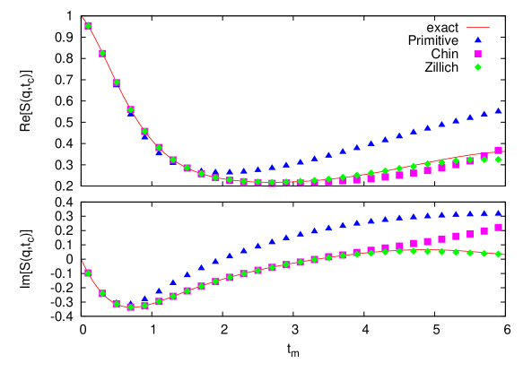
As commented in Sec. II, a relevant aspect that makes the calculation in complex time be more accurate is to use high-order actions in the evaluation of Eq. 15. We need to work with as few number of beads $M$ as possible to reach the maximum accessible time. In Fig. 1, we show results for the real and imaginary parts of $S(q,t_{c})$ for the HP as a function of $t_{m}$. The results correspond to $q=1.5$ and $\delta=\pi/9$. The line stands for the HP exact result, Lovesey

$$S(q,t_{c})=\exp\left[\frac{q^{2}}{2}\left(e^{-it_{c}}-1\right)\right]\ .$$ (16)

In the figure, we compare the exact function (16) with our QMC results obtained with a single bead, $M=1$, using different approximations for the actions employed in the evaluation of $S(q,t_{c})$. As expected, the PA is only accurate at very short times. If we consider QMC results for $S(q,t_{c})$ with a relative error of 0.4%, we notice that these are in agreement with the exact result for $t_{m}\lesssim 0.3$ and depart significantly of the exact result al larger time. Therefore, the PA is not a good choice because we would need a large number of beads to span the full time range. The results are significantly better if one uses high-order actions. In the figure, we show estimations of the real and imaginary parts using the Chin action chin and a sixth-order expansion reported by Zillich et al. Zillich10 Comparing numerical results of $S(q,t_{c})$, with the same precision as before, we notice that the Chin action reproduces the exact results up to $t_{m}\simeq 2$. However, the Chin action is in general not appropriate because of the divergence terms derived from the double commutator (notice that for the HP this divergence is reduced because this contribution produces a renormalization of the oscillator frequency). The best result is obtained using the sixth-order approximation. Zillich10 This action is able to account for the exact data up to $t_{m}\simeq 3.5$ and with the added benefit of not requiring double-commutator terms since it is based on extrapolations of PA actions with different time steps. Therefore, we have selected this action as the best option for this complex-time estimation.

A second step in our methodology is the estimation of $\varepsilon_{m}^{*}$ (see Sec. II) which determines the maximum time $t_{m}$ that can be covered with a single bead, with no significant bias coming from the small-time approximation of the action. This estimation is performed by studying the convergence of $S(q,t_{c})$, with $t_{m}=|t_{c}|$ fixed, for small values of $\varepsilon_{m}=t_{m}/M$. To perform this analysis, we have selected $\delta=\pi/2$ (imaginary time). Using a different value of $\delta$, the statistical error of $S(q,t_{c})$ tends to increase largely with the number of beads $M$ because the phase of the estimator of $S(q,t_{c})$ is proportional to $\cos\delta$ (see Appendix A), and it is not possible to give precise estimates in the limit of small $\varepsilon_{m}$.

Figure 2: (Color online) Real and imaginary parts of $S(q,t_{c})$ for HP, with $\delta=\pi/9$, as a function of $t_{m}$. The line is the exact expression (16) and the points correspond to our QMC results. The vertical lines separate the results obtained with different number of beads $M$. Where not shown, error bars are smaller than the symbol size.

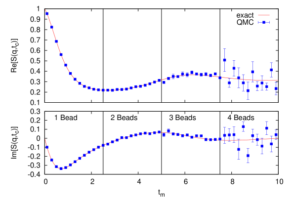
With the estimation of the accuracy of the action (for HP, we get $\varepsilon_{m}=2.5$), one can easily determine the number of complex-time beads required in the calculation of $S(q,t_{c})$ at any $t_{c}$: $M$ is the minimum integer for which the condition $|t_{c}|/M<\varepsilon_{m}^{*}$ is satisfied. Accordingly, the whole range of times $t_{m}=|t_{c}|$ is divided in different regions where $S(q,t_{c})$ is estimated with a different number of beads. In practice, $M=1$ for $t_{m}\in[0,\varepsilon_{m}^{*}]$, $M=2$ for $t_{m}\in[\varepsilon_{m}^{*},2\varepsilon_{m}^{*}]$, and so on. The results obtained with this splitting are reported in Fig. 2 for the HP and $\delta=\pi/9$. In the figure, the vertical lines separate the different intervals $[(M-1)\varepsilon_{m}^{*},M\varepsilon_{m}^{*}]$ where $S(q,t_{c})$ is calculated with the same number of beads $M$. The trends observed in this particular case are quite general. The results obtained are statistically reliable up to a maximum time $t_{m}$ which decreases when the phase $\delta$ is reduced. This feature directly implies that the maximum number of beads producing sound results is also reduced when approaching the real axis. In general, the number of beads is small but the high accuracy of the action used in the calculation makes the total covered time be quite large. In the case shown in Fig. 2, one can see that our QMC estimation is satisfactory up to $M_{\text{max}}=3$, with a total time $t_{m}=M_{\text{max}}\varepsilon_{m}^{*}=7.5$. The results with $M=4$ are spread around the exact function but with too large error bars to be used in the subsequent transform to the dynamic structure function $S(q,\omega)$.

Figure 3: (Color online) Real and imaginary parts of $S(q,t_{c})$ for HP as a function of $t_{m}$. The upper and lower lines in each panel correspond to the real and imaginary parts of the exact result (Eq. 16), respectively. The symbols correspond to our QMC results (squares: real part; triangles: imaginary part). Each panel corresponds to the calculation of $S(q,t_{c})$ for different values of the phase $\delta$ of the complex time. Error bars are smaller than the symbol size.

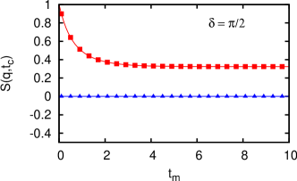
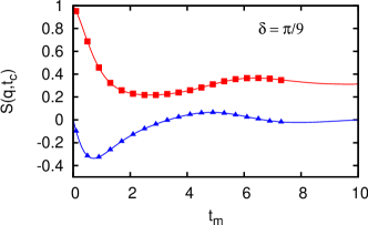
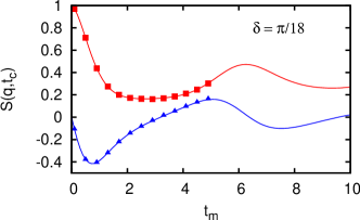
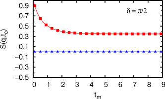
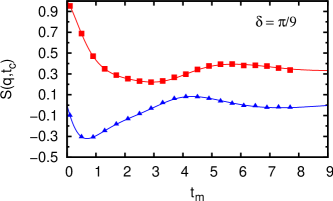
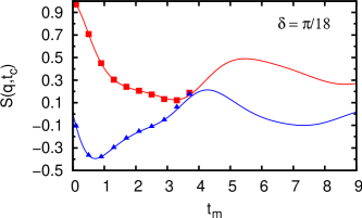
In Fig. 3, we show QMC results of the complex function $S(q,t_{c})$ for the HP and different values of the phase $\delta$, in comparison with the exact function (16). When approaching the real axis, i.e. when $\delta$ decreases, both the real and imaginary parts show an increase of their oscillatory behavior (notice that for HP, the exact $S(q,t)$ for real time is periodic), but the maximum reachable value $t_{m}$ decreases. Therefore, there is a compromise between lowering $\delta$ as much as possible and reaching times as large as possible. Our results show that the optimal phase for a posterior transform to the frequency domain is within the range $[\pi/18,\pi/9]$.

Figure 4: (Color online) Real and imaginary parts of $S(q,t_{c})$ for AP as a function of $t_{m}$. The upper and lower lines in each panel correspond to the real and imaginary parts of the exact result, respectively. The symbols correspond to our QMC results (squares: real part; triangles: imaginary part). Each panel corresponds to the calculation of $S(q,t_{c})$ for different values of the phase $\delta$ of the complex time. Error bars are smaller than the symbol size.

Proceeding in a similar way we have applied our method to the study of the correlation function for a particle in an AP. The results for the real and imaginary parts of $S(q,t_{c})$ are shown in Fig. 4 for different values of the phase $\delta$ ranging from $\pi/2$ (imaginary time) down to $\pi/36$. Our Monte Carlo results are compared with exact ones obtained by numerical integration over the eigenstates of the Hamiltonian (differently to the HP case, an analytical form for the $S(q,t_{c})$ of the AP is not known). The QMC estimation of the complex-time correlation functions shows similar accuracy to the one achieved for the HP case. Similarly to HP, we recover for the AP the exact results up to a maximum value of the modulus of the complex time $t_{m}$. Beyond this value, which decreases with $\delta$, the statistical errors grow significantly, making any estimation of $S(q,t_{c})$ not reliable. Again, a good compromise between statistical fluctuations and approaching the real axis as close as possible locates the optimal values of the phase in the same range than in the HP case, $\delta\in[\pi/18,\pi/9]$.

Once we have found the working window, the next step is to make the inversion from complex-time to energies. Our goal is to calculate the dynamic response $S(q,\omega)$ and compare the results with the exact function for both the HP and AP. To this end, we have applied the inversion technique described in the previous Section. A preliminary point is to know up to which extent the inversion procedure can influence the results in the energy domain. In the case of purely imaginary-time data, several inversion methods have been used, Boninsegni96 ; Sandwik98 ; Mishchenko00 ; Vitali10 the majority of them being of stochastic nature. This inverse Laplace transform is normally mapped to a multidimensional optimization problem. The ill-posed nature of this inversion can lead to results that can depend on the method employed.

Figure 5: (Color online) Dynamic structure function $S(q,\omega)$ for the HP at $q=1.5$. Diamonds correspond to the exact values and and circles and squares with errorbars to the results derived from the QMC results for $S(q,t_{c})$. The circles are obtained using the method described in Sec. II and the squares using a standard simulated annealing schedule. Left panel: imaginary time ($\delta=\pi/2$). Right panel: complex time ($\delta=\pi/9$).

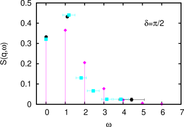
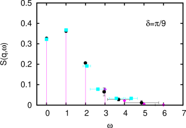
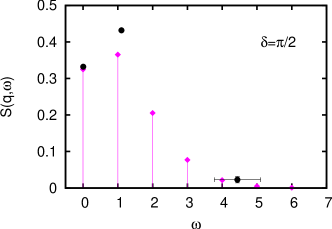
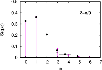
In Fig. 5, we compare results obtained for $S(q,\omega)$ in the HP problem using the inversion method discussed in the previous Section and a standard simulated annealing algorithm. In the figure, the exact result Lovesey

$$S(q,\omega)=e^{-q^{2}/2}\,\sum_{n=0}^{\infty}\frac{1}{2^{n}n!}q^{2n}\delta(n-\omega)$$ (17)

is also plot with vertical lines. This comparison is made for two cases: imaginary-time data ($\delta=\pi/2$) and complex-time results with $\delta=\pi/9$. As it has been commented, the inversion from imaginary time to the frequency domain is an ill-posed problem and thus the results can show differences depending on the selected method. This is shown in Fig. 5 (left panel): the inversion obtained from the stochastic simulated annealing method and the one discussed in Sec. II produce slightly different predictions for the higher transition lines, while they both agree on the first and second peaks, although the latter has a total strength that is $\sim 15$% off from the exact value in both cases. None of the high transition lines is well reproduced by any of the two models. In the same figure (right panel), we compare the results from both inversion methods for $\delta=\pi/9$. In this case, the inversion works on complex-time data which shows a richer structure. This significantly reduces the ill-posed character of the inversion and thus the results obtained with both methods look much more similar than in the $\delta=\pi/2$ case. Our results show that the three main peaks are well reproduced and the fourth one is approximated, slightly better using the non stochastic method which has been computed averaging over a larger data set.

Figure 6: (Color online) Dynamic structure function $S(q,\omega)$ for the HP at $q=1.5$. Diamonds correspond to the exact values (17) and circles with errorbars to the results derived from the QMC results for $S(q,t_{c})$. The inversion uses complex-time data calculated at the phases $\delta$ reported in each panel.

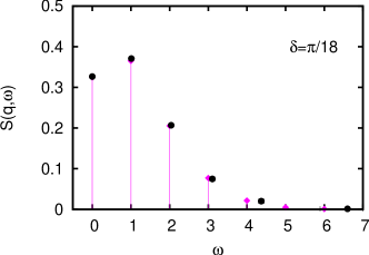
The results that we have obtained for the HP dynamic response at $q=1.5$ are reported in Fig. 6. The different panels contain reconstructions from imaginary-time data ($\delta=\pi/2$) and complex-time correlation factors estimated at decreasing values of the phase, down to $\delta=\pi/18$. At $\delta=\pi/2$ we recover the first peak (energy and strength) and approximate the second one. In other words, only the lowest-energy mode is accurately reproduced. It is worth noticing that this is the overall trend observed in transformations from purely imaginary-time data. By progressively introducing a real component in the correlation factor, i.e., by decreasing the phase $\delta$, the quality of the dynamic response improves significantly. As one can see, for $\delta=\pi/9$ one gets the first four modes with their respective strengths in nice agreement with the exact values. By reducing even more the phase down to $\delta=\pi/18$ we are able to reduce the variance of the data but no additional (higher) energies are resolved. Notice, however, that the strength of the peaks beyond the first four ones is much smaller.

Figure 7: (Color online) Dynamic structure function $S(q,\omega)$ for the AP at $q=1.5$. Diamonds correspond to the exact values and circles with errorbars to the results derived from the QMC results for $S(q,t_{c})$. The inversion uses complex-time data calculated at the phases $\delta$ reported in each panel.

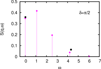
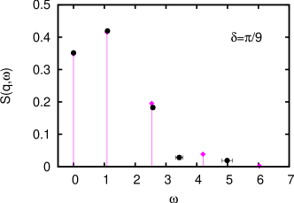
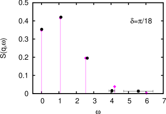
The same analysis has been carried out for the AP. Our results of the dynamic structure functions are contained in Fig. 7. With imaginary-time data, we are able to reproduce only the first peak. By decreasing the phase $\delta$ the dynamic response improves progressively. At $\delta=\pi/9$, the three main modes and their respective strengths are in close agreement with the exact results. For the smallest value $\delta=\pi/18$, we can even resolve the fourth mode whose strength is already quite small. Again, the gain of working with complex-time correlation factors becomes evident.

Figure 8: (Color online) Dynamic structure function $S(q,\omega)$ for the HP at $q=5$. Diamonds correspond to the exact values (17) and the curve corresponds to the results derived from our QMC results. Left panel: imaginary time ($\delta=\pi/2$). Right panel: complex time ($\delta=\pi/9$).

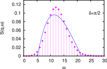
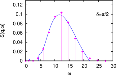
When the momentum $q$ increases, the number of modes contributing to $S(q,\omega)$ also increases, shifting the strength to higher energies. When $q$ is large enough, the dynamic response is centered around the free atom recoil energy $\omega_{R}=\hbar^{2}q^{2}/(2m)$. glyde We have calculated the dynamic response for the HP and AP at $q=5$. Our results are reported in Figs. 8 and 9 for HP and AP, respectively. The theoretical response shows in both cases, but somehow more clearly in the HP one, a distribution of modes nearly symmetric around the recoil energy. The results obtained for the HP are reported in Fig. 8 where we compare two cases, $\delta=\pi/2$ and $\delta=\pi/9$. Our results are shown with a continuous curve since our resolution does not allow for a clear separation of the individual excitation energies. Nevertheless, in the case of using complex time ($\delta=\pi/9$) the curve precisely reproduces the envelope of the exact spectrum plotted as vertical lines of strength $h_{i}$ given by

$$h_{i}=\frac{1}{\Delta\omega_{i}}\>\intop_{\omega_{i}-\Delta\omega_{i}/2}^{\omega_{i}+\Delta\omega_{i}/2}S(q,\omega)\,d\omega$$ (18)

located at the exact frequency modes $\omega_{i}$, with $\Delta\omega_{i}=(\omega_{i+1}-\omega_{i-1})/2$. Using just imaginary time produces results which are significantly worse. Similar conclusions are drawn from the results for the AP reported in Fig. 9. The results at $\delta=\pi/2$ are able only to localize the signal of $S(q,\omega)$ around $\omega_{R}$, but they cannot reproduce the shape of the spectral function. On the other hand, our results at $\delta=\pi/9$ match almost perfectly the exact dynamic response.

Figure 9: (Color online) Dynamic structure function $S(q,\omega)$ for the AP at $q=5$. Diamonds correspond to the exact values and the curve to the results derived from the QMC results for $S(q,t_{c})$. Left panel: imaginary time ($\delta=\pi/2$). Right panel: complex time ($\delta=\pi/9$).

IV Conclusions

The goal of this work is to propose a new QMC strategy aimed at the study of the dynamic response of quantum systems at zero temperature. In quantum Monte Carlo methods, the evolution of configurations is carried out in purely imaginary time, both at zero and finite temperatures, in an attempt to describe the main properties of quantum systems with high accuracy. Unfortunately, dynamics in real time is not accessible and the usual approach to get information on the dynamic response has been to reconstruct it from purely imaginary-time correlation factors. However, the ill-posed character of the inverse Laplace transform of noisy data makes this procedure quite uncertain and with multiple solutions.

Our work is an attempt of progressing in a different way, that is, to reduce the ill-posed nature of the process by inverting data containing more information than the smooth signal observed in imaginary-time. Working in the zero-temperature limit, where quantumness is unavoidable, we have devised a strategy based on the PIGS method to sample complex-time correlation factors. Our method consists in the sampling of paths connecting configurations distributed according to the ground-state wave function and, in particular, the calculation of the correlation function in complex time over the sampled paths. The use of high-order actions for the propagation in complex time has proven to be crucial to get reliable data within a time window which naturally shrinks when the real axis is approached. Optimizing the phase $\delta$ of the complex time, we have shown that, in the two model problems studied, we are able to improve significantly the calculated dynamic structure factor $S(q,\omega)$. Both at low and high $q$ the description of the dynamics is significantly improved in comparison with the usual imaginary time approach. Nevertheless, additional effort is needed to confirm the usefulness of the proposed method to problems in two and three dimensions and with more particles. Work is in progress in our group to extend this formalism to many-particle systems.

Appendix A

In this Appendix, we report the explicit expressions for the estimator $O_{A}(x_{0},\ldots,x_{M})$ appearing in Eq. 8 using different actions and having chosen to sample the paths $\{x_{1},x_{2},\ldots,x_{M-1}\}$ with $p_{\text{path}}(x_{0},x_{1},\ldots,x_{M})$ defined in Eq. 4. In general, $O_{A}$ is a complex number that can be rewritten in the form

$$O_{A}(x_{0},\ldots,x_{M})=\frac{\prod_{k=1}^{M}G(x_{k},x_{k-1};\varepsilon_{c})}{p_{\text{path}}(x_{0},x_{1},\ldots,x_{M})}=\prod_{k=1}^{M}\frac{G(x_{k},x_{k-1};\varepsilon_{c})}{G_{\text{free}}(x_{k},x_{k-1};\tau_{s})}\equiv\exp(C)\exp(iA)\ ,$$ (19)

with $\varepsilon_{c}=\varepsilon_{m}e^{-i\delta}$. The terms $C$ and $A$ are respectively the logarithm of the modulus and the phase of the complex number $O_{A}$, and their formula depends on the approximation scheme chosen for the complex-time propagator.

In the primitive action (PA) approximation, introducing the propagator $G_{\text{PA}}$ in Eq. 19 we get

$$C_{\text{PA}}=\sum_{k=1}^{M}\left[-\frac{(x_{k}-x_{k-1})^{2}}{4\lambda}\left(\frac{\sin\delta}{\varepsilon_{m}}-\frac{1}{\tau_{s}}\right)-\varepsilon_{m}\frac{V(x_{k})+V(x_{k+1})}{2\hbar}\sin\delta\right]$$ (20)

and

$$A_{\text{PA}}=\sum_{k=1}^{M}\left[\frac{(x_{k}-x_{k-1})^{2}}{4\lambda\varepsilon_{m}}\cos\delta-\varepsilon_{m}\frac{V(x_{k})+V(x_{k+1})}{2\hbar}\cos\delta\right]\ .$$ (21)

In Chin’s approximation (CA) the propagator is given by

$$G_{\text{CA}} = \prod_{j=0}^{3}\exp\left(i\frac{(x_{k,j+1}-x_{k,j})^{2}}{4\lambda t_{j}\varepsilon_{c}}\right)\exp\left(-i\frac{V(x_{k,j})+V(x_{k,j+1})}{2\hbar}v_{j}\varepsilon_{c}\right)$$ (22)

$$\times\exp\left(i\frac{u_{0}}{3}\frac{W(x_{k,j})+W(x_{k,j+1})}{2\hbar}\varepsilon_{c}^{3}\right)\ ,$$

with a generalized potential $W(r)$, due to the double commutator $[\hat{V},[\hat{K},\hat{V}]]$, and parameters $t_{j}$, $v_{j}$, and $u_{0}$ reported in Ref. Sakkos09, . Introducing this propagator in Eq. 19, we can find the functions $C_{\text{CA}}$ and $A_{\text{CA}}$,

$$C_{\text{CA}} = \sum_{j=1}^{4}\left[\left(-\frac{(x_{k,j+1}-x_{k,j})^{2}}{4\lambda t_{j}}\right)\left(\frac{\sin\delta}{\varepsilon_{m}}-\frac{1}{\tau_{s}}\right)+\right.$$ (23)

$$\left(-\varepsilon_{m}v_{j}\frac{V(x_{k,j+1})+V(x_{k,j})}{2\hbar}\right)\sin\delta+$$

$$\left.\left(\varepsilon_{m}^{3}\frac{u_{0}}{3}\frac{W(x_{k,j+1})+W(x_{k,j})}{2\hbar}\right)\sin(3\delta)\right]$$

and

$$A_{\text{CA}} = \sum_{j=1}^{4}\left[\left(\frac{(x_{k,j+1}-x_{k,j})^{2}}{4\lambda t_{j}\varepsilon_{m}}\right)\cos\delta+\right.$$ (24)

$$\left(-\varepsilon_{m}v_{j}\frac{V(x_{k,j+1})+V(x_{k,j})}{2\hbar}\right)\cos\delta+$$

$$\left.\left(\varepsilon_{m}^{3}\frac{u_{0}}{3}\frac{W(x_{k,j+1})+W(x_{k,j})}{2\hbar}\right)\cos(3\delta)\right]$$

Unfortunately, for $\delta<\pi/3$, the term with $\varepsilon_{m}^{3}$ in the expression of $C_{\text{CA}}$ (23) is positive, and then $\exp(C_{\text{CA}})$ can become exceedingly large and spoil the calculation.

In order to circumvent this problem, we have worked with the sixth-order expansion Zillich10

$$e^{\varepsilon_{c}\hat{H}} \simeq \frac{64}{45}e^{\varepsilon_{c}\hat{V}/8}e^{\varepsilon_{c}\hat{K}/4}e^{\varepsilon_{c}\hat{V}/4}e^{\varepsilon_{c}\hat{K}/4}e^{\varepsilon_{c}\hat{V}/4}e^{\varepsilon_{c}\hat{K}/4}e^{\varepsilon_{c}\hat{V}/4}e^{\varepsilon_{c}\hat{K}/4}e^{\varepsilon_{c}\hat{V}/8}$$ (25)

$$-\frac{4}{9}e^{\varepsilon_{c}\hat{V}/4}e^{\varepsilon_{c}\hat{K}/2}e^{\varepsilon_{c}\hat{V}/2}e^{\varepsilon_{c}\hat{K}/2}e^{\varepsilon_{c}\hat{V}/4}+\frac{1}{45}e^{\varepsilon_{c}\hat{V}/2}e^{\varepsilon_{c}\hat{K}}e^{\varepsilon_{c}\hat{V}/2}\ ,$$

which is built without double-commutator terms. This expansion corresponds to a linear combination of expansions approximated with PA over the same time $\varepsilon_{c}$ but with different time steps (precisely, $\varepsilon_{c}/4$ in the first term, $\varepsilon_{c}/2$ in the second term and $\varepsilon_{c}$ in the third term). Therefore, the complete formula for the exponent $C_{\text{ZA}}$ and for the phase $A_{\text{ZA}}$ in the Zillich approximation are easily obtained from $C_{\text{PA}}$ and $A_{\text{PA}}$ (Eqs. 20 and 21) calculated for different values of $\varepsilon_{c}$.

Appendix B

We discuss in this Appendix the method that we have followed to find the optimal regularization parameter (see Sec. II.B). Given the spectral function $S_{\text{INV}}(\omega,a)$ obtained inverting a series of QMC data for the complex-time correlation function $C_{\text{QMC}}(t_{c})$ with a certain regularization parameter $a$, we calculate the complex-time correlation function $C_{\text{INV}}(t_{c},a)$ obtained from the integral transform of $S_{\text{INV}}(\omega,a)$:

$$C_{\text{INV}}(t_{c},a)=\int d\omega e^{-it_{c}\omega}S_{\text{INV}}(\omega,a)\ .$$ (26)

Then we calculate the residual $\chi^{2}$ between $C_{\text{QMC}}(t_{c})$ and $C_{\text{INV}}(t_{c},a)$ as a function of the regularization parameter $a$. When $a$ is large, the regularization procedure modifies the inversion process up to the point that $C_{\text{INV}}(t_{c},a)$ starts to differ from the previous Monte Carlo data $C_{\text{QMC}}(t_{c})$, thus showing an increase in $\chi^{2}$. For very small $a$, the noise in the Monte Carlo data is largely amplified and the inversion procedure itself starts to produce meaningless results, giving rise once again to the increase in $\chi^{2}$. A plot of the total residual $\chi^{2}$ versus the regularization parameter $a$ shows a minimum, as shown in Fig. 10 for the case of the AP data at $q=1.5$ and $\delta=\pi/4$.

Figure 10: Residual $\chi^{2}$ between $C_{\text{QMC}}(t_{c})$ and $C_{\text{INV}}(t_{c},a)$ as a function of the regularization parameter $a$. The data corresponds to the calculation of the density correlation function $S(q,t_{c})$ (Eq. 15) in complex time $t_{c}=t_{m}e^{-i\delta}$ for the AP at $q=1.5$ and $\delta=\pi/4$.

In the best scenario, with high quality Monte Carlo data, an optimal regularization parameter may allow avoiding both problems. In any case, the full inspection of the inversion landscape for several values of the regularization parameter is a quick calculation.

References

- (1) D.M. Ceperley, Rev.Mod. Phys, 67, 279 (1995).
- (2) A. Sarsa, K.E. Schmidt, and W.R. Magro, J. Chem Phys, 113, 1366 (2000).
- (3) Y. Kwon, D. M. Ceperley, and R. M. Martin, Phys. Rev. B 58, 6800 (1998).
- (4) G. E. Astrakharchik, J. Boronat, J. Casulleras, and S. Giorgini, Phys. Rev. Lett. 93, 200404 (2004).
- (5) J. Cao and G. A. Voth, J. Chem. Phys. 99, 10070 (1993).
- (6) R. Craig and D. E. Manolopoulos, J. Chem. Phys. 121, 3368 (2004).
- (7) E. Krotscheck, in Microscopic Quantum Many–Body Theories and their Applications, Series “Advances in Quantum Many–Body Theories”, Vol. 7, pp. 265 - 328, Eds. A. Fabrocini, S. Fantoni, and E. Krotscheck (World Scientific, 2002).
- (8) F. Mazzanti, R. E. Zillich, G. E. Astrakharchik, and J. Boronat, Phys. Rev. Lett. 102, 110405 (2009).
- (9) A. Macia, D. Hufnagl, F. Mazzanti, J. Boronat, and R. E. Zillich, Phys. Rev. Lett. 109, 235307 (2012).
- (10) G. E. Astrakharchik, J. Boronat, E. Krotscheck, and T. Lichtenegger, J. Phys.: Conf. Ser. 529, 012009 (2014).
- (11) J. Kaipio and E. Somersalo, Statistical and Computational Inverse Problems (Springer-Verlag, New York, 2004).
- (12) M. Jarrell and J.E. Gubernatis, Phys. Rep. 269, 133 (1996).
- (13) M. Boninsegni and D.M. Ceperley, J. Low. Temp. Phys 104, 339 (1996).
- (14) A. Sandwik, Phys. Rev. B 57 10287 (1998).
- (15) A.S. Mishckenko, N.V. Prokof’ev, A. Sakamoto, and B.V.Svistunov, Phys. Rev. B 62, 6317 (2000).
- (16) E. Vitali, M. Rossi, L. Reatto, and D.E. Galli, Phys. Rev. B 82, 174510 (2010).
- (17) A. Roggero, F. Pederiva, and G. Orlandini, Phys. Rev. B 88, 094302 (2013).
- (18) P. Schofield, Phys. Rev. Lett. 4, 239 (1960).
- (19) D. Thirumalai and B. J. Berne, J. Chem. Phys. 81, 2512 (1984).
- (20) R. Feynman, Statistical mechanics: a set of lectures, Frontiers in Physics (W.A. Benjamin, 1972).
- (21) N. Chakrabarti, T. Carrington Jr., and Benoit Roux, Chem. Phys. Lett. 293, 209 (1998).
- (22) G. Krilov, E. Sim, and B.J. Berne, J. Chem. Phys. 114 1075 (2001).
- (23) E. Sim, G. Krilov, and B.J. Berne, J. Phys. Chem. A 105, 2824 (2001).
- (24) G. Krilov, E. Sim, and B.J. Berne, J. Chem. Phys. 268, 21 (2001).
- (25) A. Nakayama, and N. Makri, J. Chem. Phys. 125, 024503 (2006).
- (26) J. Kegerreis, A. Nakayama, and N. Makri, J. Chem. Phys. 128, 184509 (2008).
- (27) V. Jadhao and N. Makri, J. Chem. Phys. 129, 161102 (2008).
- (28) S. Bonella, M. Monteferrante, C. Pierleoni, and G. Ciccotti, J. Chem. Phys. 133, 164104 (2010).
- (29) S. Bonella, M. Monteferrante, C. Pierleoni, and G. Ciccotti, J. Chem. Phys. 133, 164105 (2010).
- (30) S. A. Chin and C. R. Chen, J. Chem. Phys. 117, 1409 (2002).
- (31) R. E. Zillich, J. M. Mayrhofer, and S. A. Chin, J. Chem. Phys. 132, 044103 (2010).
- (32) R. Rota, J. Casulleras, F. Mazzanti, and J. Boronat, Phys. Rev. E 81, 016707 (2010).
- (33) Stephen W. Lovesey, Theory of Neutron Scattering from Condensed Matter, Vol. 1 (Clarendon Press, Oxford, 1984).
- (34) E. L. Pollock and D. M. Ceperley, Phys. Rev. B 30, 2555 (1984).
- (35) M. Sprik, M. L. Klein, and D. Chandler, Phys. Rev. B 31, 4234 (1985).
- (36) M. Takahashi and M. Imada, J. Phys. Soc. Jpn. 53, 3765 (1984).
- (37) K. Sakkos, J. Casulleras, and J. Boronat, J. Chem. Phys. 130, 204109 (2009).
- (38) A. Neumaier, SIAM Review 40, 636 (1998).
- (39) A. N. Tikhonov, Soviet Math. Dokl. 4, 1035 (1963).
- (40) Henry R. Glyde, Excitations in Liquid and Solid Helium (Clarendon Press, Oxford, 1994).