Passive scalars: mixing, diffusion and intermittency
in helical and non-helical rotating turbulence

Abstract

We use direct numerical simulations to compute structure functions, scaling exponents, probability density functions and turbulent transport coefficients of passive scalars in turbulent rotating helical and non-helical flows. We show that helicity affects the inertial range scaling of the velocity and of the passive scalar when rotation is present, with a spectral law consistent with $\sim k_{\perp}^{-1.4}$ for the passive scalar variance spectrum. This scaling law is consistent with the phenomenological argument presented in Imazio and Mininni (2012) for rotating non-helical flows, wich states that if energy follows a $E(k)\sim k^{-n}$ law, then the passive scalar variance follows a law $V(k)\sim k^{-n_{\theta}}$ with $n_{\theta}=(5-n)/2$. With the second order scaling exponent obtained from this law, and using the Kraichnan model, we obtain anomalous scaling exponents for the passive scalar that are in good agreement with the numerical results. Intermittency of the passive scalar is found to be stronger than in the non-helical rotating case, a result that is also confirmed by stronger non-Gaussian tails in the probability density functions of field increments. Finally, Fick’s law is used to compute the effective diffusion coefficients in the directions parallel and perpendicular to the rotation axis. Calculations indicate that horizontal diffusion decreases in the presence of helicity in rotating flows, while vertical diffusion increases. We use a mean field argument to explain this behavior in terms of the amplitude of velocity field fluctuations.

I Introduction

The study of passive scalar advection, mixing and diffusion by anisotropic turbulence has gained more and more relevance over the years. Nowadays, it is well known that passive scalars share similarities with three-dimensional Navier-Stokes turbulence Sreenivasan (1991); Warhaft (2000), presenting a direct cascade, anomalous scaling and intermittency Kraichnan (1994); Falkovich et al. (2001). Moreover, the study of passive scalar mixing in turbulent anisotropic flows is of interest in a wide variety of geophysical and astrophysical problems, such as the transport of chemical elements in rotating stars Schatzman (1997); Charbonnel et al. (1992); Rudiger and Pipin (2001), the geodynamo Roberts and Glatzmaier (2000), vertical transport and diffusion in the oceans Rotunno and Bryan (2001); Osborn (1980), and the transport of polutants and aerosols in the atmosphere Csanady (1973).

Turbulent transport of passive scalars in rotating flows was previously studied in Brandenburg et al. (2009); Imazio and Mininni (2012, 2013a), although it has received less attention than the transport of passive scalars in isotropic turbulence Warhaft (2000); Falkovich et al. (2001); Celani et al. (2004). Moreover, the effect of helicity in the passive scalar transport in rotating flows has been practically ignored so far. It is known that helicity plays a key role in many problems such as in the dynamo effect Komm et al. (2008); Rudiger et al. (2010), and the effect of flow helicity in the transport of passive vectors has been the subject of study in astrophysics for many years Moffat (1970). Results in Moffat (1983); Chkhetiani et al. (2006) for isotropic turbulence indicate that passive scalar transport is sensitive to whether the flow is helical or not. In laminar flows, and in particular in biological flows, it has been found that helicity enhaces transport and mixing Elperin et al. (2000a).

As helicity affects the direct cascade of energy in rotating flows Mininni and Pouquet (2009), leading to a steeper energy spectrum, it is to be expected that the passive scalar cascade to smaller scales should also be affected by the presence of helicity (see, e.g., Imazio and Mininni (2013b)). From this point two questions naturally arise, which this work tries to answer: Is intermittency and the anomalous scaling of the passive scalar changed by the presence of helicity? And how is the transport and mixing of the passive scalar affected? While the former question can be answered by computing scaling exponents for rotating flows with and without helicity, the latter requires quantification of the turbulent transport in directions parallel and perpendicular to the rotation axis.

The aim of this paper is then to characterize the turbulent scaling, transport and diffusion of passive scalars in rotating helical flows. To this end, we use data from direct numerical simulations of the Navier-Stokes equations in a rotating frame plus the advection-diffusion equation for a passive scalar. We use a spatial resolution of $512^{3}$ grid points in a regular periodic grid.

The analisys is divided in two parts. First, to study the effect of helicity in the turbulent scaling laws of the passive scalar, we calculate velocity and passive scalar spectra. We compute structure functions for the velocity and the scalar using an axisymmetric decomposition, and consider the corresponding scaling exponents to quantify intermittency in each field. We also calculate probability density functions (PDFs) for velocity field and passive scalar increments. As for non-helical rotating turbulence (see Imazio and Mininni (2013b)), we find that the passive scalar is more anisotropic than the velocity field at small scales. However, unlike the non-helical rotating case, the passive scalar variance follows a spectral law consistent with $\sim k_{\perp}^{-1.4}$, where $k_{\perp}$ denotes wave vectors perpendicular to the rotation axis. This scaling is shallower than the one found in the non-helical rotating case Imazio and Mininni (2013b), and is correctly predicted by a simple phenomenological relation for the energy and passive scalar variance spectral indices. The passive scalar in the presence of helicity also becomes more intermittent than in the non-helical rotating case.

Secondly, to study passive scalar diffusion, we compute effective anisotropic transport coefficients using the method used first in Vincent et al. (1996) for stratified flows, and later in Imazio and Mininni (2013a) for rotating non-helical flows. Effective transport coefficients are obtained by studying the diffusion of an initial concentration of the passive scalar, and calculated using Fick’s law by measuring the average concentration and average spatial flux of the scalar as a function of time. For isotropic flows, we confirm that helicity increases turbulent diffusion (when compared with non-helical flows), in good agreement with previous studies and theoretical predictions Moffat (1983); Chkhetiani et al. (2006). In the presence of rotation, the overall effect of rotation (irrespectively of the content of helicity of the flow) is to decrease horizontal diffusion, while vertical diffusion remains approximately the same as in the isotropic case. Helicity further decreases horizontal diffusion, but slightly increases vertical diffusion (compared with the non-helical rotating case). The decrease in horizontal diffusion is explained using a simple model for turbulence diffusivity based on the amplitude of the small scale velocity fluctuations.

II Set up and simulations

II.1 Equations and numerical method

Data analyzed in the following sections stems form direct numerical simulations of the incompressible Navier-Stokes equations for the velocity ${\bf u}$ in a rotating frame, and of the advection-diffusion equation for the passive scalar $\theta$, given by

$$\partial_{t}{\bf u}+{\bf u}\cdot\nabla{\bf u}=-2{\bf\Omega}\times{\bf u}-\nabla p+\nu\nabla^{2}{\bf u}+{\bf f},$$ (1)

$$\nabla\cdot{\bf u}=0,$$ (2)

$$\partial_{t}{\theta}+{\bf u}\cdot\nabla{\theta}=\kappa\nabla^{2}{\theta}+\phi.$$ (3)

Here $p$ is the pressure divided by the mass density (taken to be uniform in all simulations), $\nu$ is the kinematic viscosity, and $\kappa$ is the scalar diffusivity. Also, ${\bf f}$ is an external force that drives the turbulence, $\phi$ is the source of the scalar field, and ${\bf\Omega}=\Omega\hat{z}$ is the rotation angular velocity.

To solve Eqs. (1)-(3) we use a parallel pseudospectral code in a three dimensional domain of linear size $2\pi$ with periodic boundary conditions Gómez et al. (2005); Mininni et al. (2011). The pressure is obtained by taking the divergence of Eq. (1), using the incompressibility condition given by Eq. (2), and solving the resulting Poisson equation. The equations are evolved in time using a second order Runge-Kutta method. The code uses the $2/3$-rule for dealiasing, and as a result the maximum resolved wavenumber is $k_{max}=N/3$, where $N$ is the number of grid points in each direction. All simulations are well resolved, in the sense that the Kolmogorov dissipation wavenumbers for the kinetic energy and passive scalar variance, respectivelly $k_{\nu}$ and $k_{\kappa}$, are smaller than the maximum wavenumber $k_{max}$ at all times. More details of the numerical procedure can be found in Imazio and Mininni (2012).

II.2 Dimensionless numbers and parameters

We will characterize the simulations using as dimensionless numbers the Reynolds, Peclèt, and Rossby numbers, defined as usual respectively as

$$\textrm{Re}=\frac{UL}{\nu},$$ (4)

$$\textrm{Pe}=\frac{\nu}{\kappa}\textrm{Re},$$ (5)

$$\textrm{Ro}=\frac{U}{2L\Omega},$$ (6)

where $U$ is the r.m.s. velocity, and $L$ is the forcing scale of the flow defined as $2\pi/k_{F}$ with $k_{F}$ the forcing wave number. In all simulations $U$ is close to unity in the turbulent steady state, and the kinematic viscosity is $\nu=6\times 10^{-4}$. The molecular scalar diffusivity is set equal to the kinematic viscosity for all runs, resulting in $\textrm{Pe}=\textrm{Re}$.

II.3 Initial conditions and external forcing

We performed a set of non-helical simulations and a set of helical simulations with varying Rossby numbers (see Table 1). In all cases, we first conducted a simulation solving only Eqs. (1) and (2) (i.e., the incompressible Navier-Stokes equations without a passive scalar), starting from the fluid at rest (${\bf u}=0$), and applying a random isotropic external mechanical forcing ${\bf f}$ to reach a turbulent steady state. This turbulent steady state was integrated for at least $13$ turnover times. The mechanical forcing ${\bf f}$ used to sustain the turbulent velocity field was a superposition of Fourier modes with random phases, delta-correlated in time, with tuneable injection of helicity using the methods described in Ref. Pouquet and Patterson (1978).

The procedure described above resulted in several runs as listed in Table 1, with runs named with the letter “A” corresponding to simulations for wich the forcing inyected zero mean helicity, and runs labeled as “B” corresponding to runs with maximal injection of helicity. The final state of the velocity field in the turbulent steady state of these runs was used as initial condition for multiple runs in which the external mechanical forcing ${\bf f}$ was maintained, but a passive scalar was injected either as an initial concentration $\theta(t=0,{\bf x})$, or randomly injected in time using the source $\phi$.

These two different ways to inject the passive scalar depended on the properties of the scalar that were studied. To characterize scaling laws and intermittency of the passive scalar in rotating helical and non-helical flows, the source term $\phi$ was used to reach a turbulent steady state in the variance of the scalar as well as in the kinetic energy. To this end, the source $\phi$ was chosen as a superposition of Fourier modes with random phases, delta-correlated in time, injected at the same wavenumbers $k_{F}$ used in the mechanical forcing ${\bf f}$.

Instead, to study passive scalar turbulent diffusion, and to compute effective transport coefficients, we turned off the source term in Eq. (3) (i.e., we set $\phi=0$). We then imposed two different initial conditions for the passive scalar, and integrated the velocity field and the passive scalar from those conditions to characterize horizontal and vertical diffusion. In each case, we used as initial condition Gaussian profiles as follows:

$$\theta(t=0,x_{i})=\theta_{0}e^{-(x_{i}-\mu)^{2}/\sigma^{2}},$$ (7)

where $i=1$ or 3 (i.e., the initial profile can be a function solely of $x_{1}=x$, or solely of $x_{3}=z$), $\mu=\pi$ (the profile is centered in the middle of the box, with the box of length $2\pi$), and $\sigma=1$. When $x_{1}=x$ is used, this allows us to study the diffusion of the initial profile in the direction perpendicular to rotation (or “horizontal”), while when $x_{3}=z$ is used, we study diffusion in the direction parallel to rotation (or “vertical”). For a few runs, we verified explicitly that the diffusion in the $x$ and $y$ directions was the same (to be expected as rotating flows tend to be axisymmetric). These runs with no forcing and with Gaussian initial profiles for the scalar will be labeled with a subindex indicating the dependence of the initial profile (e.g., runs labeled $A1_{x}$ or $A1_{z}$ indicate the run $A1$ was continued with an initial Gaussian profile for $\theta$ that depends respectively on $x$ or on $z$).

Table 1: Parameters used for the simulations: $k_{F}$ is the forcing wave number, $\Omega$ is the rotation rate, Ro is the Rossby number, $\nu$ is the kinematic viscosity, Re is the Reynolds number, and $H=\left<{\bf u}\cdot\nabla\times{\bf u}\right>$ is the mean helicity. Note that runs labeled with “A” have helicity fluctuating around zero, while runs labeled with “B” have non-zero helicity.

Run	$k_{F}$	$\Omega$	Ro	$\nu$	Re	$H$
A1	2	$0$	$\infty$	$6\times 10^{-4}$	$525$	$0$
A2	2	$8$	$0.02$	$6\times 10^{-4}$	$525$	$0$
A3	2	$16$	$0.01$	$6\times 10^{-4}$	$525$	$0$
B1	2	$0$	$\infty$	$6\times 10^{-4}$	$525$	$\approx 2$
B2	2	$8$	$0.02$	$6\times 10^{-4}$	$525$	$\approx 2$
B3	2	$16$	$0.01$	$6\times 10^{-4}$	$525$	$\approx 2$

III Turbulent scaling laws

In this section we present numerical results for the energy and passive scalar spectra, structure functions, and PDFs for helical and non-helical rotating flows. To get the results in this section, the simulations in Table 1 were continued forcing the velocity and the passive scalar, to reach a turbulent steady state in both quantities. We first present the methods used to analyze the data, then presents the results for the spectra and inertial range scaling laws, and finally we characterize intermittency using structure functions and PDFs. We also compare the data with predictions from a simple phenomenological model, and from Kraichnan model for the passive scalar.

III.1 Methods

In this first part of the paper, the analisys consist on the characterization of flow anisotropy, scaling laws, and intermittency. To this end we consider power spectra, structure functions, and PDFs of passive scalar and velocity field increments for all runs.

As a result of the anisotropy introduced by rotation, we consider reduced perpendicular energy and passive scalar spectra, namely $E(k_{\perp})$ and $V(k_{\perp})$. These reduced spectra are defined by summing the power of all (velocity or passive scalar) modes in Fourier space over cylindrical shells with radius $k_{\perp}$, with their axis aligned with the direction of the rotation axis.

To compute structure functions and PDFs, field increments must be defined first. Given the preferred direction introduced by rotation, it is natural to consider an axisymmetric decomposition for the increments. In general, the longitudinal increments of the velocity and the increments of the passive scalar fields are defined respectively as

$$\delta u({\bf x},{\bf l})=\left[{\bf u}({\bf x}+{\bf l})-{\bf u}({\bf x})\right]\cdot\frac{{\bf l}}{|{\bf l}|},$$ (8)

$$\delta\theta({\bf x},{\bf l})=\theta({\bf x}+{\bf l})-\theta({\bf x}),$$ (9)

where the increment ${\bf l}$ can point in any direction. Structure functions of order $p$ are then defined as

$$S_{p}({\bf l})=\left\langle|\delta u({\bf x},{\bf l})|^{p}\right\rangle,$$ (10)

for the velocity field, and as

$$T_{p}({\bf l})=\left\langle|\delta\theta({\bf x},{\bf l})|^{p}\right\rangle,$$ (11)

for the passive scalar field. Here, brackets denote spatial average over all values of ${\bf x}$.

These structure functions depend on the direction of the increment (i.e., they do not assume any symmetry in the flow). In simulations without rotation, the field is isotropic and the $SO(3)$ decomposition is used to calculate the isotropic component of the structure functions Arad et al. (1998); Biferale and Vergassola (2001); Biferale and Procaccia (2005). In the rotating case, due to the axisymmetry of the flow, we will consider only increments perpendicular to $\hat{z}$ (the rotation axis), and increments parallel to $\hat{z}$. We denote the former increments using $l_{\perp}$, the latter with $l_{\parallel}$, and we follow the procedure explained in detail in Mininni and Pouquet (2010); Imazio and Mininni (2012) to average over several $l_{\perp}$ directions.

This procedure to average Eqs. (10) and (11) over several directions can be summarize as follows. Velocity and passive scalar structure functions are computed from Eqs. (8) and (9) using $26$ different directions for the increments l, generated by integer multiples of the vectors $(1,0,0)$, $(1,1,0)$, $(2,1,0)$, $(3,1,0)$, $(0,1,0)$, $(-1,1,0)$, $(-1,2,0)$, $(-2,1,0)$, $(-1,2,0)$, $(-1,3,0)$, $(-3,1,0)$, $(-1,3,0)$ (all vectors are in units of grid points in the simulations), the $13$ vectors obtained by multiplying them by $-1$, and the two vectors $(0,0,\pm 1)$ for the translations in $z$. Once all structure functions were calculated, the perpendicular structure functions $S_{p}(l_{\perp})$ and $T_{p}(l_{\perp})$ are obtained by averaging over the $24$ directions in the $x-y$ plane, and the parallel structure functions $S_{p}(l_{\parallel})$ and $T_{p}(l_{\parallel})$ can be computed directly using the generators in the $z$ direction.

For all runs, this procedure was applied to $N_{s}$ snapshots of the velocity and of the passive scalar fields, separated by at least one turnover time each. For large enough Reynolds number, the structure functions are expected to show inertial range scaling, i.e., we expect that for some range of scales $S_{p}\sim l_{\perp}^{\xi_{p}}$ and $T_{p}\sim l_{\perp}^{\zeta_{p}}$, where $\xi_{p}$ and $\zeta_{p}$ are, respectively, the scaling exponents of order $p$ of the velocity and scalar fields. Scaling exponents shown bellow are calculated for all the snapshots analyzed in each simulation, and averaged over time. Errors are then defined as the mean square error; e.g., for the passive scalar exponents, the error is

$$e_{\zeta_{p}}=\frac{1}{N_{s}}\sqrt{\sum_{i=1}^{N_{s}}\left(\zeta_{p_{i}}-\overline{\zeta_{p}}\right)^{2}},$$ (12)

where $\zeta_{p_{i}}$ is the slope obtained from a least square fit for the $i$-th snapshot, and $\overline{\zeta_{p}}$ is the mean value averaged over all snapshots. The error in the least square calculation of the slope for each snapshot is much smaller than this mean square error and neglected in the propagation of errors. Extended self-similarity Benzi et al. (1993a, b) is not used to obtain the scaling exponents.

Figure 1: (a) Reduced perpendicular passive scalar variance spectrum for run B3 (rotating and helical, solid) and for run A3 (rotating and non-helical, dashed). (b) Reduced perpendicular energy spectrum for run B3 (solid) and for run A3 (dashed).

III.2 Energy and passive scalar spectra

In the presence of rotation and in the absence of helicity, the spectral behavior of the passive scalar is strongly anisotropic and quasi-two dimentional Imazio and Mininni (2012). As previously shown in Imazio and Mininni (2012), $E(k_{\perp})\sim k_{\perp}^{-2}$ for the velocity field and $V(k_{\perp})\sim k_{\perp}^{-3/2}$ for the passive scalar. The presence of helicity in rotating flows affects the cascade of energy and of the passive scalar to smaller scales. Numerical simulations in Mininni and Pouquet (2009) showed that, when helicity is present in rotating flows, the direct cascade of helicity dominates over the direct cascade of energy in the inertial range. This is the result of the development of an inverse cascade of energy, which leaves less energy available for the system to transfer to small scales. Assuming the direct cascade of helicity is dominant, a spectrum $E(k_{\perp})H(k_{\perp})\sim k_{\perp}^{-4}$ is obtained from dimensional arguments Mininni and Pouquet (2009). In other words, if the energy spectrum satisfies $E(k_{\perp})\sim k_{\perp}^{-n}$, then the helicity must follow a spectrum $H(k_{\perp})\sim k_{\perp}^{4-n}$. As a result, the energy spectrum becomes steeper as the flow becomes more helical, with the limit of a spectral index $n=2.5$ for the energy in the case of a turbulent flow with maximum helicity (in practice, this limit cannot be attained since in a flow with maximum helicity the nonlinear term becomes negligible, resulting in no net energy transfer).

Figure 2: Reduced perpendicular energy spectrum compensated by $k_{\perp}^{-2.2}$ (solid), reduced perpendicular passive scalar spectrum compensated by $k_{\perp}^{-1.4}$ (dashed), and reduced perpendicular helicity spectrum compensated by $k_{\perp}^{-1.8}$ (dash-dotted) in run B3 (with rotation and helicity).

Figure 1 shows the energy and passive scalar reduced perpendicular power spectra for runs A3 and B3 (both runs with rotation, and respectively without and with net helicity). The kinetic energy spectrum is steeper in the presence of helicity, compatible with $E(k_{\perp})\sim k_{\perp}^{-2.2}$ scaling, while the passive scalar is close to $V(k_{\perp})\sim k_{\perp}^{-1.4}$ scaling. Although resultion is moderate in these simulations (see Imazio and Mininni (2012) for more detailed studies of spectral scaling), the scaling laws can be further confirmed in Fig. 2, where compensated energy and passive scalar spectra for run B3 are shown. In Fig.  2 we also present the helicity spectrum compensated by $k_{\perp}^{-1.8}$ (to confirm that the helicity spectral index and energy spectral index add to 4). Similar scaling laws were observed in the rest of the helical rotating runs listed in Table 1.

Following the phenomenological argument presented in Imazio and Mininni (2012), we can explain the effect of helicity in the scaling of the passive scalar spectrum. From Eq. (3), the passive scalar flux $\sigma$ can be estimated as

$$\sigma\sim\frac{\theta_{l_{\perp}}^{2}u_{l_{\perp}}}{l_{\perp}},$$ (13)

If we assume that the passive scalar has a direct cascade with constant flux $\sigma$ in the inertial range, then the passive scalar power spectrum $V(k_{\perp})\sim\theta_{l_{\perp}}^{2}/k_{\perp}$ can be estimated, using Eq. (13), as

$$V(k_{\perp})\sim\frac{\sigma l_{\perp}^{2}}{u_{l_{\perp}}}.$$ (14)

For an energy spectrum $E(k_{\perp})\sim k_{\perp}^{-n}$, and therefore for a characteristic velocity at scale $l$ satisfying $u_{l_{\perp}}\sim l_{\perp}^{1-n}$, the passive scalar spectrum in Eq. (14) results

$$V(k_{\perp})\sim\sigma l_{\perp}^{\frac{5-n}{2}}\sim\sigma k_{\perp}^{-\frac{5-n}{2}}.$$ (15)

Therefore, the spectral index for the passive scalar inertial range is

$$n_{\theta}=\frac{5-n}{2}.$$ (16)

This simple phenomenological argument was proposed in Imazio and Mininni (2012) to take into account the effect of rotation in the spectrum of the passive scalar. Here we confirm that this argument remains valid in the presence of helicity in the rotating flow. Moreover, when rotation is zero, we recover $n_{\theta}=5/3$, in good agreement with the Kolmogorov scaling previously observed for passive scalars in isotropic turbulence (see, e.g., Warhaft (2000)).

Figure 3: Averaged axisymmetric structure functions (only for $l_{\perp}$ increments) up to seventh order in run B3 (rotating and helical) for (a) the passive scalar, and (b) the velocity field.

III.3 Structure functions and scaling exponents

Structure functions and scaling exponents for the passive scalar in non-helical rotating flows were studied in detail in Imazio and Mininni (2012). As a result, here we focus on the simulations with helical forcing. Figure 3 shows the axisymetric and perpendicular (i.e., only for perpendicular increments $l_{\perp}$) structure functions for the passive scalar and for the velocity field up to seventh order for run B3. Each curve corresponds to an average over $N_{s}=8$ snapshots of the turbulent steady state of the simulation. The structure functions show a range of scales with approximately power-law scaling at intermediate scales, while at the smallest scales approach the $\sim l^{p}$ scaling expected for a smooth field in the dissipative range.

Figure 4: Axisymmetric second order structure functions for run B3 (helical with rotation) for (a) the passive scalar, and (b) the velocity field. In both panels solid lines correspond to the parallel structure functions, while dashed lines correspond to the perpendicular structure functions. Slopes indicated as references correspond to the time average of the scaling exponents, obtained from a best fit in the inertial range of the structure functions at different times.

Figure 4 shows a detail for the same run of the passive scalar and velocity field second-order perpendicular structure functions, respectively $T_{2}(l_{\perp})$ and $S_{2}(l_{\perp})$, as well as the structure functions for increments parallel to the rotation axis, $T_{2}(l_{\parallel})$ and $S_{2}(l_{\parallel})$. Stronger anisotropy is observed at small scales for the passive scalar than for the velocity field, manifested as a larger difference between $T_{2}(l_{\parallel})$ and $T_{2}(l_{\perp})$ than between $S_{2}(l_{\parallel})$ and $S_{2}(l_{\perp})$. Also, an inertial range with power-law scaling can be identified at intermediate scales in $T_{2}(l_{\perp})$ and $S_{2}(l_{\perp})$. The range of scales is consistent with the wavenumbers of the inertial range in the corresponding spectra. The slopes indicated as a reference in Fig. 4 correspond to the time average of the second-order scaling exponents, obtained from a best fit in the inertial range of all structure functions at different times. The second-order scaling exponents (in the perpendicular direction) are $\zeta_{2}=0.41\pm 0.01$ for the passive scalar, and $\xi_{2}=1.22\pm 0.01$ for the velocity field. These values are in good agreement with the spectra $V(k_{\perp})\sim k^{1.4}$ and $E(k_{\perp})\sim k^{2.2}$, wich from dimensional analysis lead to $T_{2}(l_{\perp})\sim l_{\perp}^{0.4}$ and $S_{2}(l_{\perp})\sim l_{\perp}^{1.2}$. From the curves in Fig. 3, scaling exponents can also be computed for lower and higher orders. Based on the amount of statistics available, velocity and passive scalar exponents in the direct cascade range were computed for all runs up to the seventh order.

Figure 5: Scaling exponents (with error bars) as a function of the order $p$ in simulations of helical rotating turbulence, for the velocity field (triangles for run B2 and stars for run B3, both with helicity and with decreasing Rossby number), and for the passive scalar (diamonds for run B2 and squares for run B3). The solid line corresponds to the linear scaling expected for the velocity field exponents in the absence of intermittency, while the dash-dotted line corresponds to non-intermittent scaling for the passive scalar exponents. The dotted and dashed lines correspond to Kraichnan’s model with $\zeta_{2}=0.4$ and respectively with $d=2$ and with $d=3$.

Figure 5 shows the resulting velocity scaling exponents $\zeta_{p}$, and passive scalar exponents $\xi_{p}$, for runs B2 and B3 (both helical, with $\textrm{Ro}=0.02$ and $0.01$ respectively). Linear (non-intermittent) scalings for $\zeta_{p}$ and for $\xi_{p}$ are shown as a reference, based on the values of the second-order exponents $\zeta_{2}$ and $\xi_{2}$. In Fig. 5 we also show the the prediction of the Kraichnan model Kraichnan (1994), which is a model for the advection and diffusion of a passive scalar in a random, delta-correlated in time velocity field in a space with dimensionality $d$. The scaling exponents for the passive scalar in this model are

$$\zeta_{p}=\frac{1}{2}\left[\sqrt{2d\zeta_{2}p+(d-\zeta_{2})^{2}}+(d-\zeta_{2})\right].$$ (17)

For the curves in Fig. 5, these exponents were evaluated with the value of $\zeta_{2}$ obtained from the simulations, and using either $d=2$ or $d=3$.

Scaling exponents for the velocity field are similar in both runs. The second-order velocity field exponent is $\xi_{2}=1.22\pm 0.02$ for run B2, and $\xi_{2}=1.23\pm 0.01$ for run B3. The velocity field exponents display the well-known deviations from linear scaling associated with intermittency, more evident for the higher order exponents and in the simulation with larger Rossby number (i.e., smaller rotation rate). The deviation from strict scale invariance is often quantified in terms of the intermittency exponent $\mu=2\xi_{3}-\xi_{6}$, which for these runs is $\mu=0.6\pm 0.2$ for run B2, and $\mu=0.2\pm 0.1$ for run B3. The decrease in the values of $\mu$ suggest a reduction of intermittency with increasing rotation, as observed before in simulations and in experiments Baraud et al. (2003); M’́uller and Thiele (2007); Seiwert et al. (2008); Mininni et al. (2008, 2009); Mininni and Pouquet (2010); Imazio and Mininni (2012).

The passive scalar exponents for these two runs also display similar values.The second-order scaling exponent is $\zeta_{2}=0.41\pm 0.01$ for both runs. Deviations from linear scaling are observed, and the intermittency exponents are $\mu_{s}=0.36\pm 0.06$ for run B2, and $\mu_{s}=0.27\pm 0.04$ for run B3. For runs B2 and B3, Kraichnan’s model adjusts the numerical data best with $\zeta_{2}=0.4$ and $d=2$. The value of $d$ is compatible with quasi-bidimensionalization in the spatial distribution of of the passive scalar in the presence of rotation, as reported in the presence of rotation in Imazio and Mininni (2012).

Overall, the decrease in the values of $\mu$ observed for both the velocity field and the passive scalar indicate a reduction of intermittency with decreasing Rossby number. However, this reduction is more pronounced for the velocity field than for the passive scalar.

Figure 6: Scaling exponents (with error bars) as a function of the order $p$ in simulations of rotating turbulence with and without helicity, for the velocity (triangles for run A3 without helicity, and stars for run B3 with helicity), and for the passive scalar (diamonds for run A3, and squares for run B3).

Finally, we present a comparison between the scaling exponents in rotating turbulence with and without helicity. Figure 6 shows the velocity field and passive scalar exponents for runs A3 and B3 (respectively without and with helicity). Deviations from linear (non-intermittent) scaling are larger for the passive scalar in B3, indicating stronger intermittency in the presence of helicity.

III.4 Probability density functions

Intermittency and small scale anisotropy can be also studied considering the PDFs of the field increments. In this section we present PDFs of longitudinal increments of the $x$-component of the velocity field, as well as increments and spatial derivatives of the passive scalar concentration. Quantities shown are normalized by their variance, and a Gaussian curve with unit variance is shown as a reference.

Figure 7: Probability density functions in run B3, for five different horizontal spatial increments $l=1.6$ (solid), $0.8$ (dashed), $0.4$ (dash-dotted), $0.2$ (dash-triple-dotted), and $0.1$ (long dashes), and for (a) the passive scalar, and (b) the $x$-component of the velocity field. A Gaussian curve with unit variance is indicated by the dotted curve. As intervals are decreased, curves depart more and more from the Gaussian distribution developing stronger tails.

Figure 7 shows the PDFs of the velocity and of the passive scalar increments for four different values of the spatial increment ($l=1.6$, $0.8$, $0.4$, $0.2$, and $0.1$) in run B3 (with helicity). All the increments were considered in the $x$-direction (perpendicular to the axis of rotation, and for the velocity the $x$-component was used to build longitudinal increments. As a reference, and to compare with the values of the increments considered, the forcing scale in this runs is $\approx\pi$, and the dissipative scale is $\approx 0.05$. Therefore, increments $l=0.8$ and $0.4$ correspond to scales in the inertial range. The PDFs of velocity and passive scalar increments for $l=1.6$ are close to Gaussian, while for smaller spatial increments non-Gaussian tails develop. Note also that in the PDFs of passive scalar increments, a strong asymmetry develops for $l=0.4,0.2$ and $0.1$.

IV Turbulent diffusion

In this second part of the paper, the aim is to characterize the turbulent diffusion of the passive scalar in rotating helical turbulence, and to compare it with turbulent diffusion in non-helical rotating turbulence, as well as with turbulent diffusion in isotropic turbulence. To this end, we simulate the flows starting from an initial Gaussian profile for the concentration of the passive scalar, and we let it diffuse in directions parallel and perpendicular to the rotation axis. We then quantify effective transport coefficients by measuring the time evolution of the averaged concentration, and using Fick’s law.

Figure 8: (a) Averaged horizontal concentration $\overline{\theta}$ in run A$1_{x}$ (no rotation, no helicity) at times $t=0$ (solid), $0.5$ (dotted), $1$ (dashed), $1.25$ (dash-dotted), and $1.5$ (dash-triple-dotted). (b) Horizontal flux at the same times. (c) ${\cal D}_{x}(x,t)$ at the same times.

Figure 9: (a) Averaged horizontal concentration $\overline{\theta}$ in run B$1_{x}$ (no rotation, helical) at times $t=0$ (solid), $0.5$ (dotted), $1$ (dashed), $1.25$ (dash-dotted), and $1.5$ (dash-triple-dotted). (b) Horizontal flux at the same times. (c) ${\cal D}_{x}(x,t)$ at the same times.

IV.1 Methods

Before presenting the method used to measure the turbulent diffusion, we briefly recall how the simulations were conducted for this second study. As in the previous section, simulations in group A (see Table 1) correspond to simulations with zero mean helicity, while simulations in group B correspond to simulations with helical forcing and non-zero net helicity. As explained in Sec. IV.1, for each run in the turbulent steady state of the velocity field, the simulation was extended twice with the same parameters and mechanical forcing, but with two different initial conditions for the passive scalar: a Gaussian profile for the concentration in the $x$-direction (to study horizontal diffusion), and a Gassial profile in the $z$-direction (to study vertical diffusion). To identifie these runs, an additional subindex is used in this section to differentiate between simulations with different dependence of the initial Gaussian profile. As examples, a run labeled A$1_{x}$ stands for a simulation with the parameters of run A1 (i.e., with zero mean helicity and no rotation) and with initial profile of the passive scalar in the $x$-direction, while the label B$2_{z}$ indicates the run has helicity, rotation, and an initial dependence of the passive scalar in the $z$-direction.

Figure 10: Horizontal turbulent diffusion as a function of time for runs A$1_{x}$ (solid, no rotation and no helicity) and B$1_{x}$ (dashed, no rotation but with helical forcing).

In each of these runs, we let the initial profile diffuse for several turnover times. Meanwhile, we compute and store quantities averaged over the two directions perpendicular to the direction over which the original Gaussian profile varies. In particular, we consider the averaged passive scalar concentration $\overline{\theta}$, and the spatial passive scalar flux $\overline{\theta u_{i}}$, where $i=1$ or 3 depending on the initial dependence of the Gaussian profile, and where the averages denoted by the overbars are done over the two remaining Cartesian coordinates. Note the spatial flux $\overline{\theta u_{i}}$ represents the amount of passive scalar transported in the $i$-direction per unit of time by the fluctuating (or turbulent) velocity, since there is no mean flow in our simulations (we use delta-correlated in time random-forcing), $u_{i}$ is the fluctuating velocity.

Then, the pointwise effective turbulent diffusion coefficient is given by Vincent et al. (1996)

$${\cal D}_{i}(x_{i},t)=\frac{\overline{\theta u_{i}}}{\partial_{x_{i}}\overline{\theta}}.$$ (18)

This coefficient corresponds to how much passive scalar is transported by the fluctuating velocity per unit of variation of $\overline{\theta}$ with respect to $x_{i}$. As already mentioned, $i=1$ stands for horizontal diffusion, while $i=3$ stands for vertical diffusion, where the dependence on the direction of this coefficient is the result os the flow being anisotropic.

Figure 11: (a) Averaged horizontal concentration $\overline{\theta}$ in run B$3_{x}$, at times $t=0$ (solid), $0.25$ (dotted), $0.5$ (dashed), $0.75$ (dash-dotted), and $1$ (dash-triple-dotted). (b) Horizontal flux at the same times. (c) ${\cal D}_{x}(x,t)$ at the same times.

From Fick’s law, the actual turbulent diffusion coefficient is the average of ${\cal D}_{i}(x_{i},t)$ over the coordinate $x_{i}$, and if the system is in a turbulent steady state, over time. From Eq. (18), we can define these averaged diffusion coefficients as follows. We can first average over the coordinate $x_{i}$ to obtain a time dependent turbulent diffusion,

$${\cal D}_{i}(t)=\frac{1}{2\pi}\int_{0}^{2\pi}{\cal D}_{i}(x_{i},t)\mbox{d}x_{i},$$ (19)

and we can further average over time, to obtain the mean turbulent diffusion

$${\cal D}_{i}=\frac{1}{T}\int_{t_{0}}^{t_{0}+T}{\cal D}_{i}(t)\mbox{d}t.$$ (20)

Here, $t_{0}$ and $T$ are characteristic times of the flow. In practice, in our simulations the turbulent diffusion ${\cal D}_{i}(t)$ first grows in time as the initial Gaussian profile is mixed by the turbulence, then reaches an approximate steady state value for a few turnover times, and then decreases as the scalar becomes completely diluted (which happens after three or four turnover times).

Figure 12: Horizontal turbulent diffusion as a function of time for runs A$2_{x}$ (solid) and B$2_{x}$ (dashed) ($\textrm{Ro}=0.02$, respectively without and with helicity).

IV.2 Isotropic helical turbulence

In the absence of rotation, diffusion coeficients are expected to be isotropic, and therefore horizontal and vertical turbulent diffusion should be the same within error bars. Figure 8 shows the mean passive scalar profile $\overline{\theta}(x,t)$, the horizontal flux $\overline{\theta u_{x}}(x,t)$, and the pointwise value of ${\cal D}_{x}(x,t)$, at five different times for run A$1_{x}$ (no rotation and no net helicity).

As time evolves, the mean profile $\overline{\theta}(x,t)$ flattens and widens. The flux is antisymmetric: it is positive for $x>\pi$ and negative for $x<\pi$. This behavior for the flux is to be expected, as at $t=0$ there is an excess of passive scalar concentration at $x=\pi$ that must be transported by turbulent diffusion towards $x=0$ and towards $x=2\pi$. The pointwise value of ${\cal D}_{x}(x,t)$ fluctuates around a mean value (which increases with time), except close to $x=\pi$ where it rapidly takes very large positive and negative values as in that point $\partial_{x}\overline{\theta}$ approaches zero. The mean spatial value of ${\cal D}_{x}(x,t)$ increases to its saturation value around $t_{0}\approx 1.5$; after this time it fluctuates around its value (see more details below).

Figure 9 shows the same quantities at five different times for run B$1_{x}$ (i.e., in a simulation without rotation but with injection of net helicity). The behavior of the mean concentration of the passive scalar, the horizontal scalar flux, and the pointwise value of ${\cal D}_{x}(x,t)$ is qualitatively the same as in the non-helical run A$1_{x}$. However, the helical run displays a larger diffusion of the mean concentration of the scalar (as evidenced by the smaller maximum value of $\overline{\theta}(x,t)$ around $x=\pi$ and by the stronger tails close to to $x=0$ and $2\pi$, when curves at the same time are compared in Figs. 8 and 9). Also, the spatial flux $\overline{\theta u_{x}}$ takes larger extreme values in the helical simulation, and the spatial average of ${\cal D}_{x}(x,t)$ seems to result in larger values for the turbulent diffusion in this run.

Figure 13: Horizontal turbulent diffusion as a function of time for runs A$3_{x}$ (solid) and B$3_{x}$ (dashed) ($\textrm{Ro}=0.01$, respectively without and with helicity).

The increased turbulent diffusion in the presence of helicity is confirmed in Fig. 10, which shows the horizontal turbulent diffusion as a function of time for runs A$1_{x}$ and B$1_{x}$. In both runs ${\cal D}_{x}(t)$ grows from an initially small value to its saturation value around $t_{0}\approx 1.5$. As observed above, turbulent diffusion saturates at similar times for the helical and the non-helical case, but to a larger value in the presence of helicity. Although in isotropic turbulence helicity does not affect significantly the energy scaling Chen et al. (2003a, b); Mininni and Pouquet (2009); Imazio and Mininni (2013b), an increase in the turbulent diffusion in the presence of helicity was predicted in Chkhetiani et al. (2006). Using renormalization group techniques, the authors estimated that turbulent diffusion in a helical flow can be up to a $50\%$ larger than in a non-helical flow. In our simulations the averaged in time value of ${\cal D}_{x}(t)$ is $\approx 0.3$ for run A$1_{x}$, and $\approx 0.4$ for run B$1_{x}$, in reasonable agreement with the theoretical result.

It is worth mentioning that the same analysis was perfomed in simulations A$1_{z}$ and B$1_{z}$ (i.e., the same runs but with an initial Gaussian profile in the $z$-direction). As expected from the flow isotropy, the same behavior was obtained.

IV.3 Rotating helical turbulence

IV.3.1 Horizontal diffusion

Figure 14: Averaged vertical concentration $\overline{\theta}$ in run B$3_{z}$, at times $t=0$ (solid), $0.25$ (dotted), $0.5$ (dashed), $0.75$ (dash-dotted), and $1$ (dash-triple-dotted). (b) Horizontal flux at the same times. (c) ${\cal D}_{x}(x,t)$ at the same times.

Figure 11 shows the mean profile of the passive scalar $\overline{\theta}(x,t)$, the horizontal flux $\overline{\theta u_{x}}(x,t)$, and the pointwise value of ${\cal D}_{x}(x,t)$ at five different times for run B$3_{x}$ (helical and with $\textrm{Ro}=0.01$). In this case, note that the average profile and the flux become asymmetric, i.e., there is an excess of concentration of $\overline{\theta}(x,t)$ for $x<\pi$, and the absolute value of the flux is larger for $x<\pi$ than for $x>\pi$. This assymetry is caused by the Coriolis force and has been previously observed for rotating non-helical flows in Brandenburg et al. (2009); Imazio and Mininni (2013a). In our runs, the passive scalar at $t=0$ is concentrated in a narrow band around $x=\pi$. The average flux is thus towards positive values of $x$ for $x>\pi$ and towards negative values of $x$ for $x<\pi$ (i.e., in the direction of $-\nabla\theta$, see, for instance, Fig. 16). The Coriolis force in Eq. (1) is $-2\Omega\hat{z}\times{\bf u}$, and creates an overturning in in the $x$-$y$ plane of the initially only dependent on $x$ Gaussian profile, as will be shown later in more detail in spatial visualizations of the passive scalar. This overturning also results in the asymmetry in Fig. 11 (for more details, see also Imazio and Mininni (2013a)).

By compiting the mean value of ${\cal D}_{x}(x,t)$ over the spatial coordinate we obtain the turbulent diffusion coefficient. Figure 12 shows first the horizontal turbulent diffusion as a function of time for runs A$2_{x}$ and B$2_{x}$ (both with $\textrm{Ro}=0.02$, without and with helicity respectively), and then Fig. 13 shows the same quantity for runs A$3_{x}$ and B$3_{x}$ ($\textrm{Ro}=0.02$, without and with helicity respectively). For both rotation rates, we observe that horizontal diffusion is smaller in the presence of helicity. This result is the opposite to that observed for the isotropic runs in the previous section, for which helicity increased the turbulent diffusion.

Figure 15: Vertical turbulent diffusion as a function of time for runs A$3_{z}$ (solid) and $B3_{z}$ (dashed). The former run has no net helicity, while the latter has helical forcing.

As already mentioned, while in isotropic turbulence helicity does not affect the energy spectrum scaling Chen et al. (2003a, b); Mininni and Pouquet (2009); Imazio and Mininni (2013b), in rotating turbulence the presence of helicity results in shallower horizontal spectrum for the energy, in comparison with rotating non-helical turbulence Mininni and Pouquet (2009); Imazio and Mininni (2013b). As a result, a smaller turbulent diffusion can be expected, as small scale velocity field flutuations should be less energeting in the helical rotating case. Indeed, in most two point closure models, the turbulent diffusivity is proportional to the mean kinetic energy in the turbulent fluctuations, $\overline{u^{2}}/2$, and if the kinetic energy spectrum is steeper, then the diffusivity should decrease. A simple mean field argument can illustrate this. We can split the velocity in a mean flow $\overline{{\bf u}}$, and a fluctuating component ${\bf u}^{\prime}$, such that ${\bf u}=\overline{{\bf u}}+{\bf u}^{\prime}$. In our runs $\overline{{\bf u}}=0$, and ${\bf u}={\bf u}^{\prime}$. Splitting the passive scalar in the same way we have $\theta=\overline{\theta}+\theta^{\prime}$. Replacing in Eq. (3) and averaging we obtain

$$\frac{\partial\overline{\theta}}{\partial t}=-\nabla\cdot(\overline{{\bf u}\theta^{\prime}}),$$ (21)

and subtracting this equation from Eq. (3) we then obtain

$$\frac{\partial\theta}{\partial t}=-\nabla\cdot({\bf u}\overline{\theta}).$$ (22)

We can integrate this last equation assuming the flow is correlated over the integral eddy turnover time $\tau$, to obtain

$$\theta^{\prime}\approx-\tau\nabla\cdot({\bf u}\overline{\theta})=-\tau{\bf u}\cdot\nabla\overline{\theta},$$ (23)

where incompressibility was used. Then, replacing in Eq. (21),

$$\frac{\partial\overline{\theta}}{\partial t}\approx\frac{\partial}{\partial x_{i}}\left(\tau\overline{u_{i}u_{j}}\right)\frac{\partial\overline{\theta}}{\partial x_{i}},$$ (24)

where the coefficient $\tau\overline{u_{i}u_{j}}$ can be interpreted as a turbulent diffusion. If the flow is isotropic, then ${\cal D}\approx\tau\overline{u^{2}}$. A more refined mean field derivation of this expression can be found in Elperin et al. (2000b); Blakman and Field (2003); Brandenburg et al. (2012), while two point closure derivations can be found in Kraichnan (1976); Herring et al. (1982).

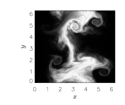
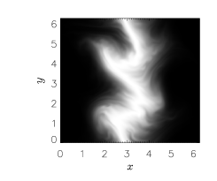
Figure 16: Passive scalar concentration in a horizontal slice of runs A$3_{x}$ (left) and $B3_{x}$ (right) at time $t=1$. Note how the initial concentration (Gaussian, centered around $x=\pi$, and independent of the $y$-coordinate) gets distorted and diffussed.

Although the argument above is only illustrative, it gives an interesting hint to the possible cause of the reduced perpendicular diffusion in helical rotating flows. As the perpendicular energy spectrum in this case is steeper than in the absence of helicity, then the smaller energy at small scales results in less mixing and diffusion.

IV.3.2 Vertical diffusion

Figure 14 shows the mean vertical passive scalar concentration $\overline{\theta}(z)$, the mean vertical flux $\overline{\theta v_{z}}(z)$, and the pointwise value of ${\cal D}_{z}(z)$ at different times in run B$3_{z}$. In this case, the profiles are more similar to those obtained in the isotropic and homogeneous case: $\overline{\theta}(z)$ and $\overline{\theta v_{z}}(z)$ are respectively symmetric and antisymmetric with respect to $z=\pi$.

As in the case of horizontal diffusion, we can obtain the vertical turbulent diffusion coefficient as a function of time by computing the mean value of ${\cal D}_{z}(z,t)$ for all values of $z$. Figure 15 shows ${\cal D}_{z}(t)$ for runs A$3_{z}$ and B$3_{z}$ (both with $\textrm{Ro}=0.01$, respectively without and with helicity). Note that horizontal turbulent diffusion is larger in the presence of helicity, even more than in the isotropic case.

IV.4 Spatial distribution and structures

Results shown above suggest that both horizontal and vertical diffusions are affected by rotation and by the presence of helicity. Figure 16 shows a horizontal slice of the passive scalar concentration in runs A$3_{x}$ and B$3_{x}$ at $t=1$ (i.e., around the time the turbulent diffusion coefficients ${\cal D}_{x}$ and ${\cal D}_{z}$ reach a turbulent steady value). As also observed in Imazio and Mininni (2013a), the initial Gaussian profile in the non-helical rotating flow (run A$5_{x}$) diffuses in time, and also bends and rotates. As previously mentioned, the overturning of the profile is caused by the Coriolis force (see also Brandenburg et al. (2009)). In the helical rotating flow (run B$3_{x}$), we also observe this overturning, although the initial profile is less diffused (as indicated, e.g., by the most extreme values in the $x$-coordinate for which a significant concentration of the passive scalar can be observed, which are larger in run A$5_{x}$).

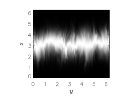
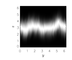
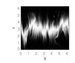
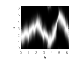
Figure 17: Passive scalar concentration in a vertical slice of runs A$3_{z}$ (left) and B$3_{z}$ (right) at time $t=0.5$ (top row), and at time $t=1.5$ (bottom row).

Diffusion in the parallel direction in rotating flows is of a different nature than vertical diffusion (see Fig. 17, which shows vertical slices of the passive scalar concentration in runs A$3_{z}$ and B$3_{z}$ at $t=0.5$ and $t=1.5$.). In the rotating non-helical case, the passive scalar initial profile is diffused in vertical stripes, created by updrafts or downdrafts inside columnar structures of the velocity field Imazio and Mininni (2013a). These columnar structures in the velocity and vorticity fields have been reported in rapidly rotating flows, and are associated with the bidimensionalization of the flow Cambon and Jacquin (1989); Waleffe (1992); Davidson et al. (2006). As time increases, the stripes observed in the passive scalar in Fig. 17 are further streched, resulting in larger mixing and diffusion. Note however that in the presence of helicity, the stripes are increased even further, in good agrement with the increased diffusion in helical flows reported above. This can be understood as the presence of helicity in the flow requires the three components of the velocity to be non-zero, resulting in a more three-dimensional flow.

V Conclusions

We analyzed data from direct numerical simulations of advection and diffusion of a passive scalar in rotating helical and non-helical turbulent flows. A total of $18$ simulations with spatial resolution of $512^{3}$ grid points was performed, using different Reynolds and Rossby numbers, and changing the forcing and initial conditions of the passive scalar, to meassure energy and passive scalar spectra, anisotropic velocity and passive scalar structure functions, probability density functions, and diffusion coefficients in the directions parallel and perpendicular to the rotations axis.

In the first part of the paper we studied scaling laws of the energy and passive scalar variance, using spectra and structure functions in the horizontal and vertical directions. We showed that helicity affects the inertial range scaling of the passive scalar, with its variance following a spectral law consistent with $\sim k_{\perp}^{-1.4}$. This scaling is shallower than the one found for passive scalars in non-helical rotating turbulence Imazio and Mininni (2013b), and consistent with a phenomenological argument that states that if the energy follows a power law $\sim k^{-n}$ in the inertial range, then the passive scalar variance should follow a power law $\sim k^{-n_{\theta}}$ with $n_{\theta}=(5-n)/2$. This argument, already proposed in Imazio and Mininni (2013b) for rotating and non rotating non-helical flows, was found here to uphold also in the presence of helicity. The study of structure functions confirms these scaling laws, and indicates that the passive scalar is more anisotropic at small scales than velocity field. Also, the passive scalar was found to be more intermittent than the velocity field, a well known result, what which becomes more pronounced in the presence of rotation and of helicity. The anomalous scaling exponents for the passive scalar can be approximated using Kraichnan’s model with the second order exponent $\zeta_{2}$ obtained from our phenomenological model, and with a dimensionality $d=2$. As in the case of rotating non-helical flows studied previously in Imazio and Mininni (2012), this value of $d$ was interpreted as a result of the quasi-bidimentionalization of the distribution of the passive scalar in the presence of rotation.

In the second part of the paper, the analisys of the effective diffusion coeficients calculated from Fick’s law show that for isotropic flows (i.e., without rotation) helicity increases turbulent diffusion, in agreement with previous models and theoretical predictions Moffat (1983); Chkhetiani et al. (2006). In the presence of rotation, results indicate that the overall effect of rotation (irrespectively of the content of helicity of the flow) is to decrease horizontal diffusion, while the effect on vertical diffusion is less pronounced. Helicity further decreases horizontal diffusion but increases vertical diffusion (compared with the non-helical rotating case). The decrease in horizontal diffusion was explained with a simple model for turbulence diffusivity based on the available energy for the small-scale turbulent fluctuations.