On the consistent treatment of the quasi-hydrostatic layers in hot star atmospheres

Abstract

Context. Spectroscopic analysis remains the most common method to derive masses of massive stars, the most fundamental stellar parameter. While binary orbits and stellar pulsations can provide much sharper constraints on the stellar mass, these methods are only rarely applicable to massive stars. Unfortunately, spectroscopic masses of massive stars heavily depend on the detailed physics of model atmospheres.

Aims. We demonstrate the impact of a consistent treatment of the radiative pressure on inferred gravities and spectroscopic masses of massive stars. Specifically, we investigate the contribution of line and continuum transitions to the photospheric radiative pressure. We further explore the effect of model parameters, e.g., abundances, on the deduced spectroscopic mass. Lastly, we compare our results with the plane-parallel TLUSTY code, commonly used for the analysis of massive stars with photospheric spectra.

Methods. We calculate a small set of O-star models with the Potsdam Wolf-Rayet (PoWR) code using different approaches for the quasi-hydrostatic part. These models allow us to quantify the effect of accounting for the radiative pressure consistently. We further use PoWR models to show how the Doppler widths of line profiles and abundances of elements such as iron affect the radiative pressure, and, as a consequence, the derived spectroscopic masses.

Results. Our study implies that errors on the order of a factor of two in the inferred spectroscopic mass are to be expected when neglecting the contribution of line and continuum transitions to the radiative acceleration in the photosphere. Usage of implausible microturbulent velocities, or the neglect of important opacity sources such as Fe, may result in errors of approximately 50% in the spectroscopic mass. A comparison with TLUSTY model atmospheres reveals a very good agreement with PoWR at the limit of low mass-loss rates.

1 Introduction

The initial mass of a star determines its evolutionary path, and is thus considered one of the most fundamental stellar parameters. Yet stellar masses derived for massive stars via spectral analyses are generally prone to large uncertainties, greatly hampering an accurate calibration of stellar masses with their spectral types and evolutionary status. The so-called “mass discrepancy” problem, which arises when comparing stellar masses obtained from spectroscopy, to orbital, wind, and evolutionary models, has been of concern to stellar physicists for a few decades (Herrero et al. 1992; Repolust et al. 2004; Massey et al. 2012). While recent studies suggest a solution of this problem over the years (Weidner & Vink 2010; Markova & Puls 2014), discrepancies still exist, especially in the range of giants to supergiants.

In principle, orbital masses are independent of stellar atmosphere models and are therefore considered to be more robust (e.g., Torres et al. 2011). However, orbital masses are only attainable in the rare case of binary systems with well-constrained inclination, usually owing to eclipses. Immense progress has also been made in the field of asteroseismology, which allows the measurement of stellar masses with very high accuracies from observed stellar pulsations. Unfortunately, the high variability in the outer layers of massive stars make the study of their pulsational behavior very difficult, often hindering an effective implementation of asteroseismological methods to massive stars (see recent review by Aerts 2014, and references therein). Indeed, spectroscopy remains the primary method to infer stellar masses for the majority of the massive stars.

The spectroscopic mass of a star is derived from its radius $R_{*}$ and surface gravity $g_{\ast}$ via $M_{\ast}=G^{-1}\,g_{\ast}\,R_{*}^{2}$, and therefore any uncertainties in $R_{*}$ and $g_{\ast}$ propagate into uncertainties in $M_{\ast}$. Except for the rare case where the angular diameter of a star can be directly measured, $R_{*}$ is derived from the luminosity $L$ and effective temperature $T_{\text{eff}}$ of the star via the Stefan-Boltzmann relation $R_{\ast}=\left(4\pi\sigma_{\text{SB}}\right)^{-1/2}\,L^{1/2}\,T_{\text{eff}}^{-2}$. Since the effective temperature can in principle be constrained with decent accuracy, the main cause for uncertainty in the stellar radius is the error in the distance $d$, which propagates in the error in $L$, according to $R_{\ast}\propto\sqrt{L}\propto d$. If the distance is well constrained and thus the spectroscopic radius is known, the stellar mass $M_{\ast}$ is directly proportional to $g_{\ast}$ and thus all uncertainties in the gravity determination propagate directly into mass uncertainties.

The gravity $g_{*}$ is by no means a directly measurable quantity. It is derived by comparing synthetic spectra from model atmospheres with observations. The surface gravity of a star determines the stratification of its atmospheric pressure, and most prominently affects the pressure-broadened wings of hydrogen and helium lines. The determination of $g_{*}$ thus relies on both the pressure broadening theory adopted, as well as the model atmosphere.

Different broadening theories can lead to systematic differences of $\sim 0.15\,$dex in inferred $\log g_{\ast}$ values, which alone corresponds to $\sim 40\%$ error in the inferred spectroscopic mass. It is an even harder task, however, to constrain the systematic errors that arise because of different assumptions and techniques in stellar atmosphere codes. The radiative pressure in massive stars depends on the stellar parameters as well as the opacity, which in turn depends on the elements, abundances, atomic data, and line Doppler widths. As we illustrate in this study, $g_{\ast}$ is highly model-dependent, and systematic errors can easily occur if the radiative pressure is not fully and consistently accounted for.

Two domains can be distinguished in the atmosphere of a massive star: a hydrostatic domain, where gravity is balanced by pressure (e.g., gas pressure, radiation pressure), and a wind domain, where the outward pressure exceeds gravity and the matter is accelerated.

The spectra of O- and B-type stars are mostly formed in the outer layers of their quasi-hydrostatic domains. For the modeling of such stars, a detailed treatment of the hydrostatic regime is imperative. Specifically, the contribution of line and continuum transitions to the total radiative pressure in the quasi-hydrostatic domain is far from negligible. Proper knowledge of the velocity field in the layers close to the stellar surface is a key ingredient for a better understanding of a variety of theoretical and observational phenomena (see, e.g., Hamann 1981; Cidale & Ringuelet 1993; Owocki & Puls 1999; Cantiello et al. 2009; Shenar et al. 2014).

In this paper, we thoroughly document the current calculation of the radiative pressure in the Potsdam Wolf-Rayet (PoWR) code (see, e.g. Gräfener et al. 2002; Hamann & Gräfener 2003) and illustrate the importance of accounting for it consistently. While we focus on the PoWR code, the major concepts and equations are representative of the majority of current state-of-the-art stellar atmosphere codes, as we illustrate in a brief comparison. We further discuss and quantify the large impact of a proper hydrostatic treatment on inferred stellar parameters, and particularly on the stellar mass $M_{\ast}$. We demonstrate the sensitivity of the radiative pressure to the Doppler width of spectral lines and to the iron abundance. Lastly, we compare our results with the plane-parallel TLUSTY O-grid models from Lanz & Hubeny (2003), which are widely used for the analysis of hot stars with negligible winds.

The structure of this paper is as follows: In Sect. 2, we briefly summarize the main assumptions of the PoWR code and thoroughly discuss the treatment of the quasi-hydrostatic domain. The outcome of our test calculations are shown and discussed in Sect. 3. In Sect. 4, we compare our spectra with corresponding TLUSTY models, before drawing the general conclusions in Sect. 5.

2 The PoWR code

2.1 The Basics

The Potsdam Wolf-Rayet models describe atmospheres of spherically symmetric stars with a stationary outflow. To achieve a consistent solution, the equations of statistical equilibrium and radiative transfer are iteratively solved to yield the population numbers without the approximation of a local thermodynamic equilibrium (non-LTE). The radiative transfer is solved in the comoving frame, which avoids simplifications such as the Sobolev approximation. After an atmosphere model is converged, the synthetic spectrum is calculated via a formal integration along emerging rays. Some description of the PoWR code can be found in Gräfener et al. (2002) and Hamann & Gräfener (2004). The temperature stratification is updated iteratively to ensure energy conservation in the expanding atmosphere, as described in Hamann & Gräfener (2003). Recently, the PoWR code has been extended by the so-called thermal balance-method, which goes back to ideas of Hummer & Seaton (1963) and Hummer (1963) and is described in detail for stellar atmospheres by Kubát et al. (1999) and Kubát (2001). This method provides better numerical stability in optically thin domains.

In the comoving frame calculations during the non-LTE iteration, we assume that the line profiles are Gaussians with a constant Doppler broadening velocity $\varv_{\text{dop}}$, which approximately accounts for the thermal and turbulent velocity. A constant broadening velocity is a well-established simplification in comoving frame methods. While PoWR uses directly a velocity $\varv_{\text{dop}}$ as input, the “Comoving Frame General” (CMFGEN) code requires three input parameters $T_{\text{dop}}$, $A_{\text{dop}}$, and $\varv_{\text{T}}$ , which are then combined to a constant velocity $\varv_{\text{dop}}=\sqrt{2\frac{k_{\text{B}}T_{\text{dop}}}{m_{\text{H}}A_{\text{dop}}}+\varv_{\text{T}}^{2}}$ (see, e.g., Martins et al. 2002, CMFGEN description). In the FASTWIND code a velocity similar to PoWR has to be given and is referred to just as mircroturbulence $\varv_{\text{turb}}$ (Puls et al. 2005).

The value of $\varv_{\text{dop}}$ is chosen such that it approximately reflects the order of the averaged thermal speed combined with the microturbulence, i.e.,

$$\varv_{\text{dop}}\approx\sqrt{\bar{\varv}_{\text{th}}^{2}+\varv_{\text{turb}}^{2}}.$$ (1)

For O and B stars typical values for $\varv_{\text{dop}}$ range between $10$ and $30\,$km/s. Only for stars without photospheric lines, such as classical Wolf-Rayet stars, higher values can be chosen to speed up the calculations without changing the emergent spectrum. The influence of $\varv_{\text{dop}}$ on an O-star model spectrum is discussed and illustrated in Sect. 3.4.

Pressure broadening is neglected during the comoving frame calculations, which is sufficient for the current applications of the PoWR models. For stars with considerably higher values of $\log g_{\ast}$, e.g. , subdwarfs, specific codes, such as the Tübingen Model-Atmosphere Package (TMAP) (e.g., Werner et al. 2003) exist which include this effect. Some codes, such as the TLUSTY code, have the option to switch on pressure broadening in the iteration if needed. In the formal integration in PoWR, detailed thermal, microturbulent and pressure broadening are accounted for in a depth-dependent manner.

The basic parameters of a PoWR model are the stellar temperature $T_{\ast}$, luminosity $L$, mass-loss rate $\dot{M}$, surface gravity $g_{*}$ and the chemical abundances. The stellar temperature $T_{\ast}$ is defined as the effective temperature of a star with the luminosity $L$ and radius $R_{\ast}$ (referred to as the “stellar radius”), defined at the Rosseland continuum optical depth $\tau_{\text{max}}=20$. The total Rosseland optical depth $\tau_{\text{Ross}}(R_{\ast})$ including lines is larger. To ensure $\tau_{\text{max}}=20$ at the inner boundary, the velocity $\varv_{\text{min}}=\varv(R_{\ast})$ is iteratively adjusted. The surface gravity $g_{\ast}$ is defined at the stellar radius $R_{*}$ via $g_{\ast}=G\,M_{\ast}\,R_{\ast}^{-2}$. For OB stars, the difference between the radius where $\tau_{\text{max}}=20$ and the “photospheric radius” at $\tau_{\text{Ross}}=2/3$ is usually very small. However, in supergiants the effective temperature can differ up to $\sim 1$ kK between these two points, and this difference in definition is apparent when compared with other studies.

The density stratification in the quasi-hydrostatic domain follows from an integration of the hydrostatic equation, thoroughly discussed in Sect. 2.2. In the wind domain, the radial wind velocity $\varv(r)$ is usually prescribed in the model by a so-called $\beta$-law

$$\varv(r)=\varv_{\infty}\left(1-\frac{R_{\ast}}{r}\right)^{\beta},$$ (2)

where $\varv_{\infty}$ is the terminal velocity of the wind, and $\beta$ is a free input parameter whose value typically ranges between $\beta=0.6$ and $\beta=2.0$ ,(e.g., Puls et al. 2008). With the mass-loss rate $\dot{M}$ specified, the density stratification $\rho(r)$ in the wind follows from the continuity equation

$$\dot{M}=4\pi r^{2}\varv(r)\,\rho(r)\text{.}$$ (3)

In the calculation, we use complex model atoms, with a superlevel approach for iron group elements (see Gräfener et al. 2002, for details), and an explicit set of quantum levels for all other elements. The detailed chemical composition for our calculations is given in Sect. 3, together with the rest of the model parameters.

We do not use any clumping in the models and instead assume a smooth wind. The potential existence of clumping in the subsonic photosphere is a constant debate in the massive star community (see, e.g., Runacres & Owocki 2002; Oskinova et al. 2007; Cantiello et al. 2009; Sundqvist & Owocki 2013). While clumping would significantly affect the derived absolute stellar parameters in any case, the goal of this work is to demonstrate effects that are independent of any clumping formalism. Therefore, we refrain from assuming a particular clumping approximation and calculate our test models (see Sect. 3) with a smooth wind.

2.2 The quasi-hydrostatic domain

The Potsdam Wolf-Rayet (PoWR) model atmosphere code was originally developed for WR stars where the emergent spectrum is formed almost exclusively in the stellar wind. For these objects, it is sufficient to treat the quasi-hydrostatic domain of WR stars with a simple barometric formula using a constant scale height

$$H_{\text{c}}:=\frac{\frac{\mathcal{R}T_{\ast}}{\mu}+\varv_{\text{turb}}^{2}}{g_{\text{eff}}\leavevmode\nobreak\ R_{\ast}},$$ (4)

in units of $R_{\ast}$ while ensuring a smooth transition of the velocity field and its gradient between the two quasi-hydrostatic domain and the wind. Here, $g_{\text{eff}}$ is the gravity corrected for radiative pressure in the hydrostatic domain (see details below), $\mu$ the mean particle mass (including electrons) in units of the hydrogen atom mass $m_{\text{H}}$, and $\varv_{\text{turb}}$ the turbulent velocity, which is a free input parameter. The parameter $\mathcal{R}$ denotes the specific gas constant for hydrogen, i.e., $\mathcal{R}=k_{\text{B}}/m_{\text{H}}$.

For a proper treatment of O- and B-star atmospheres, the barometric formula with a constant scale height is not an appropriate solution of the hydrostatic equation. The hydrostatic equation is one of the fundamental equations of stellar structure. For massive stars, one has to account for the outward radiative force acting against gravitation, yielding the radial stratification of pressure $P(r)$ in the hydrostatic domain,

$$\frac{\mathrm{d}P}{\mathrm{d}r}=-\rho(r)g(r)\left[1-\Gamma(r)\right].$$ (5)

Here, $\rho(r)$ is the mass density, $g(r)=G\,M_{*}/r^{2}$ the gravity, and $\Gamma(r)$ the ratio between the outward radiative acceleration and gravitational acceleration. The term $\left[1-\Gamma(r)\right]$ describes the effective reduction of the gravity due radiative pressure, as discussed below.

With the assumption of an ideal gas, the pressure $P$ can be expressed by

$$P(r) =\rho(r)\left[\frac{\mathcal{R}T(r)}{\mu(r)}+\varv^{2}_{\text{turb}}\right]$$ (6)

$$=\rho(r)\left[a^{2}(r)+\varv^{2}_{\text{turb}}\right]\text{,}$$ (7)

where $T$ is the electron temperature. In the second line we further introduce the sound speed

$$a(r):=\sqrt{\frac{\mathcal{R}T(r)}{\mu(r)}}$$ (8)

in order to simplify the expression. The turbulent velocity $\varv_{\text{turb}}$ is a free depth-independent input parameter reflecting a possible microturbulence. While in the formal integral the microturbulence is combined with the actual thermal velocity of each element to obtain the precise depth-dependent Doppler broadening velocity, it is not directly connected to the value of $\varv_{\text{dop}}$ used in the comoving-frame calculation. To avoid physically inconsistent situations, the value of $\varv_{\text{dop}}$ should be higher than for $\varv_{\text{turb}}$. So far this has been ensured by the user, but we are planning to implement a more detailed treatment of microtubulence in the comoving-frame calculations, also allowing for depth-dependent changes.

The current implementation allows us to compare our OB-type models with those of other stellar atmosphere codes, as they adopt similar approaches (cf. Table 1). Stellar atmosphere analyses with several codes (see, e.g., Massey et al. 2013) have demonstrated that microturbulent velocities of the order of $10$ to $20\,$km/s help to reproduce the observed spectral lines in certain parameter regimes. It is an ongoing debate whether such velocities represent a real turbulent motion in the photosphere, as originally suggested for hot stars by Struve & Elvey (1934) and prominently reintroduced by Hubeny et al. (1991), or if they are rather a “fudge factor”. Related to this open question is the discussion whether such a turbulent term should be included in the hydrostatic equation or not. In the PoWR code the term is included, but because of its currently depth-independent implementation there are no additional derivatives occuring and it merely leads to an offset of the sound speed.

For simplicity, we will set $\varv_{\text{turb}}=0$ km/s in the following calculations, but the full result can always be recovered by replacing $a^{2}$ with $a^{2}+\varv^{2}_{\text{turb}}$. Upon dividing Eq. (5) by $-\rho$, the term on the left side, which we will refer to as

$$a_{\text{press}}(r):=-\frac{1}{\rho}\frac{\mathrm{d}P}{\mathrm{d}r}$$ (9)

describes the outward acceleration due to gas pressure and turbulent motion. Thus the hydrostatic equation can be written as

$$a_{\text{press}}(r)=g(r)\left[1-\Gamma(r)\right]\text{,}$$ (10)

illustrating that in the hydrostatic domain the outward acceleration due to gas pressure has to balance gravity reduced by the radiative acceleration. In a strictly hydrostatic domain, we have therefore no net velocity, i.e., no stellar wind.

For an accurate description of an expanding stellar atmosphere, i.e., with $\varv\neq 0$, one would have to use the hydrodynamic equation, which can be written for a stationary, symmetric outflow in the following form:

$$\frac{1}{\rho}\frac{\mathrm{d}P}{\mathrm{d}r}+\varv\frac{\mathrm{d}\varv}{\mathrm{d}r} =-g(r)\left[1-\Gamma(r)\right.].$$ (11)

This means there is only one additional term in Eq. (11) compared to the hydrostatic Eq. (5). This inertia term $a_{\text{mech}}(r):=\varv\frac{\mathrm{d}\varv}{\mathrm{d}r}$ is of fundamental importance in the outer wind, but becomes negligible quickly below the sonic point. This also holds for a $\beta$-type velocity law with $\beta>0.5$ where $a_{\text{mech}}$ approaches zero for $r\rightarrow R_{\ast}$. Thus in the subsonic domain the hydrodynamic equation (11) transitions into the hydrostatic form (5) and we obtain a quasi-hydrostatic stratification.

In such a quasi-hydrostatic situation, we can still have a nonvanishing velocity, even though its value is subsonic and, as we will see in the comparison with purely hydrostatic models in Sect. 4, negligible for the observed spectrum. Furthermore this small velocity still fulfills the equation of continuity (3). This can be used to obtain the consistent solution for the velocity field in the quasi-hydrostatic domain. First, we replace the pressure gradient in $a_{\text{press}}$ with the help of Eq. (7),

$$a_{\text{press}} =-\frac{1}{\rho}\frac{\mathrm{d}P}{\mathrm{d}r}$$ (12)

$$=-\frac{\mathrm{d}a^{2}}{\mathrm{d}r}-\frac{a^{2}}{\rho}\frac{\mathrm{d}\rho}{\mathrm{d}r}.$$ (13)

We then eliminate the density in the second term by using the equation of continuity (3) and thus write

$$a_{\text{press}} =-\frac{\mathrm{d}a^{2}}{\mathrm{d}r}-a^{2}r^{2}\varv\frac{\mathrm{d}}{\mathrm{d}r}\left(\frac{1}{r^{2}\varv}\right)$$ (14)

$$=-\frac{\mathrm{d}a^{2}}{\mathrm{d}r}+\frac{2a^{2}}{r}+\frac{a^{2}}{\varv}\frac{\mathrm{d}\varv}{\mathrm{d}r}\text{.}$$ (15)

Finally, by combining Eqs. (10) and (15), we obtain an equation for the velocity gradient in the quasi-hydrostatic regime,

$$\frac{\mathrm{d}\varv}{\mathrm{d}r}=\frac{\varv}{a^{2}}\left[\frac{GM_{\ast}}{r^{2}}\left(1-\Gamma(r)\right)-\frac{2a^{2}}{r}+\frac{\mathrm{d}a^{2}}{\mathrm{d}r}\right].$$ (16)

In principle, given a value $\varv(R_{*})=\varv_{\text{min}}$ at the inner boundary, one can obtain the velocity field in the quasi-hydrostatic part via direct integration of this equation. In practice, we transform this equation and split off the main exponential trend as this turned out to work better in terms of numerical stability. Thus our solution for the quasi-hydrostatic velocity field is

$$\varv(r)=\varv_{\text{min}}\frac{a^{2}(r)}{a^{2}(R_{\ast})}\frac{R_{\ast}^{2}}{r^{2}}\exp\left(\frac{r-R_{\ast}}{H_{\text{c}}}-b(r)\right),$$ (17)

with a yet to be determined function $b(r)$. We now calculate the derivative of Eq. (17) with respect to r,

$$\frac{\mathrm{d}\varv}{\mathrm{d}r}=-\frac{2\varv}{r}+2\frac{\varv}{a^{2}}\frac{\mathrm{d}a^{2}}{\mathrm{d}r}+\varv\left[\frac{1}{H_{\text{c}}}-\frac{\mathrm{d}b}{\mathrm{d}r}\right]\text{,}$$ (18)

combine this with Eq. (16), and obtain

$$-\frac{2}{r}+\frac{1}{a^{2}}\frac{\mathrm{d}a^{2}}{\mathrm{d}r}+\frac{1}{H_{\text{c}}}-\frac{\mathrm{d}b}{\mathrm{d}r} =\frac{GM_{\ast}}{a^{2}r^{2}}\left(1-\Gamma(r)\right)-\frac{2}{r}+\frac{1}{a^{2}}\frac{\mathrm{d}a^{2}}{\mathrm{d}r}.$$ (19)

$$\frac{1}{H_{\text{c}}}-\frac{\mathrm{d}b}{\mathrm{d}r} =\frac{GM_{\ast}}{a^{2}r^{2}}\left(1-\Gamma(r)\right)$$ (20)

The righthand side of Eq. (20) is now defined as $H(r)^{-1}$, as it is analogous to the definition of $H_{\text{c}}$ (Eq. 4). Thus the numerical integration of the velocity gradient is replaced by the integration of

$$\frac{\mathrm{d}b}{\mathrm{d}r}=\frac{1}{H_{\text{c}}}-\frac{1}{H(r)}\text{.}$$ (21)

The required boundary value $b(R_{\ast})=0$ follows from the inner boundary, where it is required in Eq. (17) that $\varv(R_{\ast})=\varv_{\text{min}}$.

So far, we did not discuss what enters $\Gamma(r)$ and thus $H(r)$. In general, the letter $\Gamma$ is used to describe a ratio between a radiative acceleration and gravity. The most common use is the so-called “electron gamma”,

$$\Gamma_{\text{e}}=\frac{a_{\text{thom}}(r)}{g(r)}=\frac{\sigma_{\text{e}}}{4\pi cm_{\text{H}}G}q_{\text{ion}}(r)\frac{L}{M_{\ast}},$$ (22)

which accounts only for the radiative pressure because of scattering of free electrons. Note that $r^{2}$ cancels out in the last expression, since the acceleration because of Thomson scattering is defined as

$$a_{\text{thom}}(r):=\frac{\sigma_{\text{e}}L}{4\pi cm_{\text{H}}r^{2}}q_{\text{ion}}(r),$$ (23)

with the ionization parameter,

$$q_{\text{ion}}(r)=m_{\text{H}}\frac{n_{\text{e}}(r)}{\rho(r)}=\frac{n_{\text{e}}(r)}{n_{\text{tot}}(r)\mathcal{A}}.$$ (24)

The mean atomic mass $\mathcal{A}$ is constant in an atmosphere model. The two density factors can be replaced by the slowly varying mean particle mass $\mu(r)=\mathcal{A}\left(1+\frac{n_{\text{e}}(r)}{n_{\text{tot}}(r)}\right)^{-1}$ such that

$$q_{\text{ion}}(r)=\frac{1}{\mu(r)}-\frac{1}{\mathcal{A}}\text{,}$$ (25)

illustrating that $q_{\text{ion}}$ is nearly constant throughout the atmosphere. As a consequence, $\Gamma_{\text{e}}$ has only a very weak radial dependence.

While Eq. (22) is the common definition for $\Gamma$ in the context of the Eddington limit, it is only a fraction of the total outward radiative acceleration $a_{\text{rad}}$. Apart from the Thomson opacity corresponding to scattering of free electrons, additional opacities originate in line (bound-bound) and continua (bound-free, free-free) transitions, contributing to the total radiative acceleration. $a_{\text{rad}}$ is thus separated into three parts:

$$a_{\text{rad}}=a_{\text{thom}}+a_{\text{lines}}+a_{\text{true cont}}.$$ (26)

The last term $a_{\text{true cont}}$ refers to the acceleration originating from bound-free and free-free continuum transitions. As the electron opacity also forms a continuum, these two terms are combined and referred to as the “continuum”. In contrast, the term without electron scattering is sometimes called the “true continuum”. To avoid any confusion, we will adopt this notation in the following.

Similar to Eq. (22), we can thus define a $\Gamma,$ which corresponds to the total acceleration,

$$\Gamma_{\text{rad}}(r) :=\frac{a_{\text{rad}}(r)}{g(r)}=\frac{1}{g(r)}\frac{4\pi}{c}\frac{1}{\rho(r)}\int\limits_{0}^{\infty}\,\kappa_{\nu}(r)\,H_{\nu}(r)\,\mathrm{d}\nu,$$ (27)

where $\kappa_{\nu}$ and $H_{\nu}$ are the opacity and Eddington flux at the frequency $\nu$, respectively, and $c$ is the speed of light. This “full” $\Gamma_{\text{rad}}$ is then used in the quasi-hydrostatic domain. A similar approach was also adopted by Lanz & Hubeny (2003) in their plane-parallel TLUSTY code, which is widely used for calculating photospheric spectra of static atmospheres.

Table 1: Characteristics of different stellar atmosphere codes concerning their treatment of the (quasi-)hydrostatic regime

	PoWR	CMFGEN	FASTWIND	TLUSTY
radiative transfer	comoving frame	comoving frame	CMF/Sobolev	static (obs. frame)
blanketing	full	full	approximative	full
temperature stratification obtained by	radiative equilibrium or thermal balance	radiative equilibrium	thermal balance	radiative equilibrium
photosphere	quasi-hydrostatic	quasi-hydrostatic	quasi-hydrostatic	hydrostatic
$(\rho,\varv)$-update	consistent	injections	start iterations	$\varv\,\equiv\,0$, $\rho$ consistent
radiative acceleration used in hydrostatic eq.	full $a_{\text{rad}}$	full $a_{\text{rad}}$	$a_{\text{cont}}$ approximation	full $a_{\text{rad}}$
$\varv_{\text{turb}}$ parameter in hydrostatic eq.?	yes	yes	no	yes
domain connection	continuous $\mathrm{d}\varv/\mathrm{d}r$	$0.75\,\varv_{\text{sonic}}$	$0.1\,\varv_{\text{sonic}}$ (adjustable)	no wind domain

In contrast to $\Gamma_{\text{e}}$, which is already known at the start of a non-LTE model atmosphere calculation, with the exception of the exact value of $q_{\text{ion}}(r),$ the full $\Gamma_{\text{rad}}$ has to be calculated iteratively. The radiative acceleration is calculated from the population numbers, which in turn depend on the radiation field and also on the density which itself is connected to $\Gamma_{\text{rad}}$ via the hydrostatic equation. To ensure a consistent solution, the velocity field in the quasi-hydrostatic domain is constantly updated as soon as the hydrostatic equation is violated by more than 5%. This turned out to be sufficient in all test cases, as long as $\Gamma_{\text{rad}}(r)<1$ in the quasi-hydrostatic part. In reality, values larger than unity in the (quasi-)hydrostatic domain would reflect additional physical phenomena occurring in the photosphere (e.g., subphotospheric convection, Cantiello et al. 2009), which are not handled by our model atmospheres. The plane-parallel TLUSTY code treats only values of $\Gamma_{\text{rad}}\leq 0.9$ in the hydrostatic equation (Lanz & Hubeny 2003) as the hydrostatic equation fails for values larger than unity and numerical instabilities already occur when $\Gamma_{\text{rad}}$ gets close to this limit. We use a similar approach in PoWR for the quasi-hydrostatic equation, i.e., the value of $\Gamma_{\text{rad}}$ is limited to $0.9$ for our velocity calculations.

2.3 The quasi-hydrostatic treatment in different stellar atmosphere codes

A couple of non-LTE stellar atmopshere codes are used in the field of hot and massive stars. Widely used are CMFGEN (Hillier & Miller 1998), FASTWIND (Santolaya-Rey et al. 1997), and, in case of negligible stellar winds, TLUSTY (Hubeny & Lanz 1995b). While these codes have a lot of similarities in their concepts, they also differ in certain approaches, such as their treatment of the radiative transfer or their superlevel approach. Recent comparisons between CMFGEN and FASTWIND (Massey et al. 2013) for particular objects have shown a good agreement in the derived temperatures, but also revealed that the surface gravities derived with FASTWIND are abound $0.12\,$dex lower than with CMFGEN. As the derived surface gravities are directly connected to the treatment of the quasi-hydrostatic layers, it is of major interest to understand the difference between the codes in this regime.

Table 1 provides an overview of the features affecting the quasi-hydrostatic treatment of PoWR, CMFGEN, and FASTWIND together with the completely hydrostatic treatment in TLUSTY. The latter provides an interesting test case in the limit of negligible mass-loss rates, which will be further discussed in Sect. 4, where we compare spectra from TLUSTY models with those from PoWR. In CMFGEN, TLUSTY model atmospheres can also be used as a start approach.

The most striking difference in the quasi-hydrostatic treatment between the different wind codes (PoWR, CMFGEN, FASTWIND) is the update mechanism of the density and velocity stratification:

• In PoWR, we update the velocity field as described in Sect. 2.2 as part of the main iteration as soon as the hydrostatic equation is violated by more than 5% or the specified value of $\tau_{\text{max}}$ is missed by more than a specified $\epsilon_{\tau}$. For each update, $\Gamma_{\text{rad}}(r)$ is applied in the hydrostatic equation, using $a_{\text{rad}}(r)$ from the comoving frame (CMF) calculations. With the new velocity field given, the stratification is updated according to the equation of continuity (3).

• In CMFGEN (Hillier & Miller 1998), the hydrostatic domain is first taken from a TLUSTY model or an old CMFGEN model, but can be updated with regards to the hydrostatic equation after a first convergence of the population numbers and the radiation field. After each such stratification update, sometimes referred to as “injection”, the model iteration has to be continued to reachieve convergence (see, e.g., Martins et al. 2012, for a brief description). Similar to PoWR, the radiative acceleration used in the hydrostatic equation is taken from the CMF radiative transfer calculations.

• In FASTWIND (Santolaya-Rey et al. 1997), the line contributions are instead neglected in the quasi-hydrostatic domain and uses an approximate handling for the continuum acceleration, including both Thomson and true continuum term. This simplification allows FASTWIND to set up the quasi-hydrostatic domain in an iteration right at the start of a model, in line with the goal of the code of being significantly faster than PoWR and CMFGEN.

Furthermore, all three wind codes use a different criterion for the connection point between the quasi-hydrostatic and the wind domain. While FASTWIND and CMFGEN use a fixed fraction of the sound speed to define this connection point, PoWR puts the condition of a smooth velocity gradient between the two regimes.

Instead of treating only the quasi-hydrostatic part consistenly, one could also aim at a hydrodynamically consistent treatment throughout the whole model atmosphere, i.e., including the wind domain. These calculations are typically not included in state-of-the-art stellar atmosphere codes, especially as a prescribed $\beta$-law provides a good approximation for the outer wind regime of OB stars. A self-consistent calculation of the velocity field in the whole stellar atmosphere has been implemented as a nonstandard option in PoWR in order to discuss WR winds (Gräfener & Hamann 2005, 2008). However, such models require much longer computation times and this option is not required for the purpose, in which we focus on the quasi-hydrostatic regime. The implementation presented here is completely sufficient in achieving a self-consistent stratification of the quasi-hydrostatic layers. Nevertheless, a revised implementation of completely hydrodynamically consistent model atmospheres in the PoWR code will be addressed in detail in a future work.

2.4 The effective gravity

The hydrostatic Eq. (5) can be written in an even shorter form with the definition of the effective gravity,

$$g_{\text{eff}}(r):=\frac{GM_{\ast}}{r^{2}}\left[1-\Gamma(r)\right]\text{.}$$ (28)

To avoid any confusion, we will use $g_{\text{grav}}(r)$ instead of $g(r)$ with $g_{\ast}=g_{\text{grav}}(R_{\ast})$ to denote the full gravity from here on. The effective gravity $g_{\text{eff}}$ is a fundamental fitting parameter for O- and B-stars when comparing models with observations. The pure gravitational acceleration $g_{\text{grav}}(r)=GM_{\ast}r^{-2}$, from which the stellar mass is derived, can only be calculated if $\Gamma_{\text{rad}}$ is known. Therefore, $g_{\text{grav}}$ is model dependent. In these models an accurate treatment of the complete radiative pressure is required. Correcting the observed $g_{\text{eff}}$ for Thomson pressure $\Gamma_{\text{e}}$ only neglects a large part of the radiative pressure, and leads to an underestimated stellar mass, as we will demonstrate in Sect. 3. In the cases of negligible radiative pressures only do $\log g_{\text{grav}}$ and $\log g_{\text{eff}}$ become indistinguishable. Otherwise, spectroscopic masses are underestimated if calculated directly via $R_{\ast}^{2}\,g_{\text{eff}}/G$.

As the shape of a spectral line like H$\delta$ depends on $g_{\text{eff}}$ and not $g_{\text{grav}}$, there is a parameter degeneracy. A star with a weaker radiative pressure will produce the same line profiles as a star with a higher radiative pressure and a higher gravity.

One of the major reasons for a strong model dependency of the stellar mass is the large impact of the opacity on the radiative pressure. It is significant which opacities are taken into account in the model. Neglecting elements such as Fe or Ne will result in a lower $\Gamma_{\text{rad}}$ and is not legitimate, even if the corresponding element is not under consideration in the intended analyses. The inferred stellar mass therefore depends not only on the adopted stellar parameters, but also on the details of the model atoms.

The adopted Doppler broadening velocity $\varv_{\text{dop}}$ used in the comoving-frame calculations also has a significant impact: larger velocities allow atoms to absorb photons in a wider frequency range, and thus generally increase the radiative pressure in the atmosphere.

Even though $g_{\text{eff}}(r)$ and $\Gamma_{\text{rad}}(r)$ are calculated for each depth point in the PoWR code to fulfill the hydrostatic equation, there is a need for a certain “reference value” , which can be used for comparisons. As the emergent spectrum is mainly formed at $\tau_{\text{Ross}}\approx 2/3$ in the photosphere, the first idea would be to use $g_{\text{eff}}$ at this value. However, such a fixed point might already be located in the wind. Therefore we define a weighted mean of $\Gamma_{\text{rad}}$ as

$$\overline{\Gamma}_{\text{rad}}:=\int\limits_{\tau_{\text{max}}}^{\tau_{\text{sonic}}}\Gamma_{\text{rad}}(\tau_{\text{Ross}})\leavevmode\nobreak\ e^{-\tau_{\text{Ross}}}\leavevmode\nobreak\ \mathrm{d}\tau_{\text{Ross}}\text{.}$$ (29)

The upper limit of the integral $\tau_{\text{sonic}}$ usually denotes the optical depth of the sonic point. However, we do not allow that this value drops below $0.1$, even in the rare cases where the actual sonic point would be in such a regime. The calculated value of $\overline{\Gamma}_{\text{rad}}$ is used to relate $\log g_{\text{eff}}$ and $\log g_{\ast}=\log g_{\text{grav}}(R_{\ast})$ via

$$\log g_{\text{eff}}=\log g_{\ast}+\log\left(1-\overline{\Gamma}_{\text{rad}}\right).$$ (30)

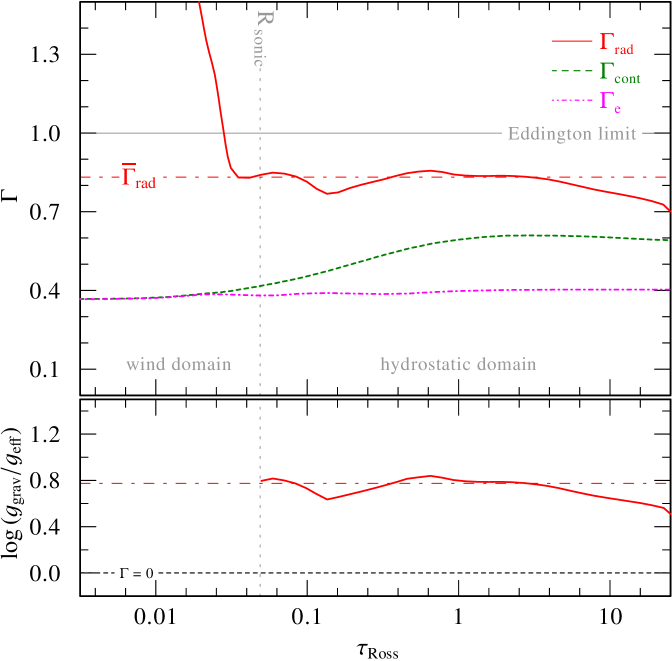
Figure 1: Radial dependence of $\Gamma_{\text{rad}}$ (red, solid line, upper panel) for our supergiant test model, plotted over the Rosseland optical depth $\tau_{\text{Ross}}$. The mean value obtained with Eq. (29) is indicated as a dashed-dotted line. For comparison, $\Gamma_{\text{e}}$ and the total continuum contribution $\Gamma_{\text{cont}}$ are also shown. In the lower panel, the difference between $g_{\text{grav}}$ and $g_{\text{eff}}$ is illustrated: the red solid curve marks the actual difference at each optical depth, while the dashed-dotted line denotes the difference using $\overline{\Gamma}_{\text{rad}}$. The gray dashed vertical line denotes the location of the sonic point.

The radial dependence of $\Gamma_{\text{rad}}$ for a supergiant test model is illustrated in Fig. 1, where it is plotted against the total Rosseland opacity. It is evident that in the quasi-hydrostatic regime not only the line transitions, but also the atomic continuum transitions cannot be neglected, while this quickly changes as soon as we enter the supersonic domain, where $\Gamma_{\text{cont}}$ consists only of $\Gamma_{\text{e}}$. One can see that the calculated value of $\overline{\Gamma}_{\text{rad}}$ is indeed representative for the difference between $g_{\text{grav}}$ and $g_{\text{eff}}$ in the photosphere. Values of $\overline{\Gamma}_{\text{rad}}$ for a series of test models are shown and discussed in Sect. 3.

The reference radius for all values of $g_{\text{eff}}$ given in this work is $R_{\ast}$. However, other radii are also used in the literature, typically $R_{\frac{2}{3}}=R\left(\tau_{\text{Ross}}=\frac{2}{3}\right)$ or the radius of the sonic point $R_{\text{s}}$. The latter roughly indicates the outer end of the quasi-hydrostatic domain. It is therefore interesting to check how much the values of $g_{\text{eff}}$ and $g_{\text{grav}}$ are affected when referring to different radii. As this effect is largest for supergiants, we examine an O-star model with $T_{\ast}=32.5\,$kK, $\log L/L_{\odot}=5.6$, $\log g_{\text{grav}}(R_{\ast})=3.25$ and $\log\dot{M}=-5.75\,$[M_⊙/yr]. For this model, we have $R_{\frac{2}{3}}=1.06\,R_{\ast}$ and the sonic point is located at $R_{\text{s}}=1.11\,R_{\ast}$, leading to differences of $0.05\,$dex and $0.09\,$dex in $\log g$. Especially the latter value is approximately what can be achieved by accurate fitting of high quality spectra and, therefore, we have to take the reference radius into account when analyzing these objects. This effect is lower for giants and dwarfs, namely on the order of $0.03\,$dex and $0.01\,$dex for the sonic point, respectively.

In the literature, the term $g_{\text{eff}}$ may not always have the same meaning. Especially when dealing with observations, it is often not clearly stated whether values termed as $\log g$ have been corrected for radiative acceleration. Values that have been corrected for centrifugal acceleration in a statistical sense are sometimes labeled as “true” gravities $g_{\text{true}}$ or $g_{\text{c}}$ with the relation

$$g_{\text{c}}=g+\frac{\left(\varv\sin i\right)^{2}}{R_{\ast}}$$ (31)

(Repolust et al. 2004). The term labeled as $g$ in this equation is sometimes called $g_{\text{eff}}$ (e.g., Massey et al. 2013). We would like to stress that this is not identical to our definition of the effective gravity in this work. The variable $g$ in (31) refers to the gravitational acceleration specified in a non-rotating stellar atmosphere model, which has not been reduced by radiative acceleration. As such, $g$ would be referred to as $g_{\text{grav}}$, following the notation of this work. Caution is therefore adviced when dealing with the term “effective gravity”, as its definition might differ significantly between different authors.

3 Results and discussion

3.1 Test model details

To illustrate the impact of accounting for the full radiative pressure consistently, we calculate a set of PoWR models for a fixed temperature of $T_{\ast}=32.5\,$kK , which corresponds to a late O-star. For this temperature, we calculate three types of models with different surface gravities, corresponding to the luminosity classes I (supergiant), III (giant), and V (dwarf). As we focus on the quasi-hydrostatic part, we adopt only schematic parameters for the wind, i.e., all models have the same terminal wind velocity of $\varv_{\infty}=2000\,$km/s. The outer model boundary is set to $100\,R_{*}$. The velocity field in the wind domain can be prescribed by a $\beta-$law with $\beta=0.8$ (see Eq. 2), which is accurate enough for our purposes as we do not want to analyze the outer wind. The luminosities are “typical” representatives of their class according to Martins et al. (2005). We chose the surface gravities similarly, but with slight adjustments of up to $0.1\,$dex, corresponding to the closest grid point in the TLUSTY O-star model grid (Lanz & Hubeny 2003) for a later comparison (see Sect. 4). We adopted mass-loss rates from Vink et al. (2000), and the wind is assumed to be smooth (no density contrast, i.e., $D=1$ in the notation of Hamann & Koesterke 1998). The chemical compositions are taken to be solar. Here, we use the abundances inferred by Grevesse & Sauval (1998) instead of the newer ones obtained by Asplund et al. (2009) to have identical values to those used in the TLUSTY O-grid. All parameters of the models are compiled in Table 2.

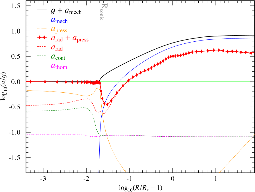
Figure 2: Acceleration stratification for a model with a consistent quasi-hydrostatic domain (Type (b) models). The wind acceleration (thick red diamond line) is compared to the repulsive sum of inertia and gravitational acceleration $g(r)$ (black line). All terms have been normalized to $g(r)$.

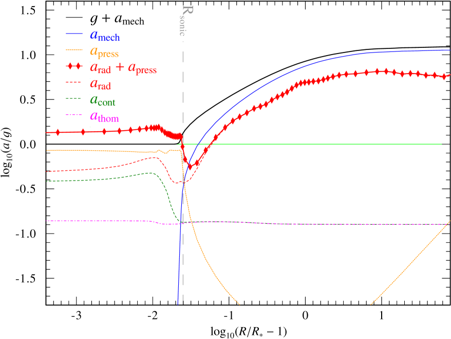
Figure 3: Same as Fig. 2, except with a velocity law in the quasi-hydrostatic domain accounting only for $\Gamma_{\text{e}}$ (Type (a) models). While the wind domain is not affected, the acceleration balance in the quasi-hydrostatic part is significantly different.

Table 2: O-star test model parameters

Luminosity class	I	III	V
$T_{*}$ [kK]	$32.5$
$\log g_{\text{eff}}$ [cm s-2]	$2.47$	$3.02$	$3.79$
$\log g_{\text{grav}}$ [cm s-2]	$3.25$	$3.50$	$4.00$
$\overline{\Gamma}_{\text{rad}}$	$0.83$	$0.67$	$0.39$
$\Gamma_{\text{e}}$	$0.40$	$0.22$	$0.07$
$R_{*}$ [$R_{\odot}$]	$20.0$	$14.1$	$8.1$
$\log\dot{M}$ [$M_{\odot}\,\text{yr}^{-1}$]	$-5.75$	$-6.25$	$-7.1$
$\log L$ [$L_{\odot}$]	$5.60$	$5.30$	$4.82$
$M_{\ast}$ [$M_{\odot}$]	$25.9$	$23.0$	$24.1$
$\beta$	0.8
$\varv_{\infty}$ [km/s]	2000
$\varv_{\text{turb}}$ [km/s]	10
$\varv_{\text{dop}}$ [km/s]	20
$X_{\text{H}}$	$0.704$
$X_{\text{He}}$	$0.282$
$X_{\text{C}}$	$2.78\times 10^{-3}$
$X_{\text{N}}$	$8.14\times 10^{-4}$
$X_{\text{O}}$	$7.56\times 10^{-3}$
$X_{\text{Mg}}$	$6.45\times 10^{-4}$
$X_{\text{Al}}$	$5.56\times 10^{-5}$
$X_{\text{Si}}$	$6.96\times 10^{-4}$
$X_{\text{P}}$	$6.10\times 10^{-6}$
$X_{\text{S}}$	$4.79\times 10^{-4}$
$X_{\text{Fe}}$	$1.34\times 10^{-3}$

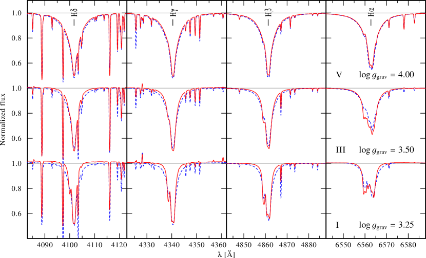
Figure 4: Balmer line profiles of H$\delta$ (left) to H$\alpha$ (right) for test models with fixed $g_{\text{grav}}$. The spectra from the (a)-type models with a quasi-hydrostatic stratification calculated using only the Thomson term $\Gamma_{\text{e}}$ are shown as blue dashed line. The red solid lines display the profiles from the (b)-type models accounting for the full radiative term $\Gamma_{\text{rad}}$.

Table 3: O-star test model type overview

Model type	(a)	(b)	(c)
$g_{\text{grav}}$	fixed	fixed	calculated
$\Gamma$	$\Gamma_{\text{e}}$	$\overline{\Gamma}_{\text{rad}}$	$\Gamma_{\text{e}}$
$g_{\text{eff}}$	calculated	calculated	fixed

For each of the three luminosity classes, we calculate three models, which we refer to as (a), (b), and (c) in the following, making nine models in total period. Models (a) and (b) have a fixed $g_{\text{grav}}$ , which corresponds to the respective luminosity class and differ only in the treatment of the radiative acceleration in the quasi-hydrostatic part: models (a) are only calculated with $\Gamma_{\text{e}}$ , while models (b) include the full $\Gamma_{\text{rad}}$, i.e., they account for the complete radiative pressure. Typical examples are shown in Fig. 2 and Fig. 3, where we plot the acceleration stratifications for a dwarf (class V) model. One can see that Fig. 2 shows the consistent (b)-model, where the sum of the total radiative acceleration and gas pressure equals gravitation in the quasi-hydrostatic domain. The result of the (a)-model is shown in Fig. 3. Now only $\Gamma_{\text{e}}$ and gas pressure are taken into account for the hydrostatic equation and thus the sum of the total radiative acceleration and gas pressure is larger than the local gravity in the subsonic part. The outer parts of both models are very similar as both use the same prescribed $\beta$-velocity law.

In models (c), like in models (a), we account only for the Thomson term $\Gamma_{\text{e}}$ in the quasi-hydrostatic domain, but instead of specifying $\log g_{\text{grav}}$, we specify the effective gravity $\log g_{\text{eff}}$ and adopt its value from the corresponding model (b), calculated from Eq. (30). An overview of the basic similarities and differences between all three model types is given in Table 3. Since models (b) and (c) of a given luminosity class have the same effective gravity, the wings of pressure-broadened lines are expected to be identical in both models. However, because of different treatment of the quasi-hydrostatic domain, the actual surface gravities $g_{\text{grav}}$ and spectroscopic masses $M_{\ast}$ implied from both models will differ.

3.2 Comparison with fixed $g_{\text{grav}}$

Figure 4 illustrates the impact of accounting for the full radiative pressure on prominent Balmer lines (left to right: H$\delta$, H$\gamma$, H$\beta$, H$\alpha$) for dwarfs (upper panels), giants (middle panels), and supergiants (lower panels). The impact of either including only the Thomson term $\Gamma_{\text{e}}$ (model a, blue dashed lines) or including the full radiative term $\Gamma_{\text{rad}}$ (model b, red solid lines) can be seen in the line wings. Because of their larger outward pressures, the quasi-hydrostatic domains of models (b) are less dense than those of models (a), and, as a consequence, the line wings obtained by models (b) are narrower. For the same reason, the value of $g_{\text{eff}}$ is always smaller in models (b) compared to models (a) (see below).

A further inspection of Fig. 4 reveals that the difference between models (a) and (b) increases with luminosity class. A look at Eq. (27) reveals that lower values of $\log g_{\text{grav}}$ will increase $\Gamma_{\text{rad}}$, which is indeed much larger for the supergiant than for the dwarf. Even though the difference between $\Gamma_{\text{rad}}$ and $\Gamma_{\text{e}}$ is not getting much stronger with lower $\log g_{\text{grav}}$, as $\Gamma_{\text{e}}$ also changes proportional to $R_{\ast}^{2}$, both values are significantly larger for the supergiant and thus the difference in the derived $g_{\text{eff}}$ value increases, which is reflected in the increasing line wing difference in Fig. 4.

Even for our dwarf models ($\log g_{\text{grav}}=4.0$, upper panels), where the dashed and solid lines can only barely be distinguished, we obtain a difference of $\Delta\log g_{\text{eff}}=0.21\,$dex when accounting for the full radiative pressure via $\Gamma_{\text{rad}}$ ($\log g_{\text{eff}}=3.97$ for model (a) vs. $\log g_{\text{eff}}=3.78$ for model (b)). For our giant models ($\log g_{\text{grav}}=3.5$, middle panels) the difference increases to $0.37\,$dex ($3.39$ vs. $3.02$). Finally, for the supergiant models ($\log g_{\text{grav}}=3.25$, lower panels), a formidable difference of $0.56\,$ dex ($3.03$ vs. $2.47$) is obtained. Even though the impact on the spectral appearance of the hydrogen lines might not be particularly striking in Fig. 4, the differences in the corresponding values of $\log g_{\text{eff}}$ are quite remarkable.

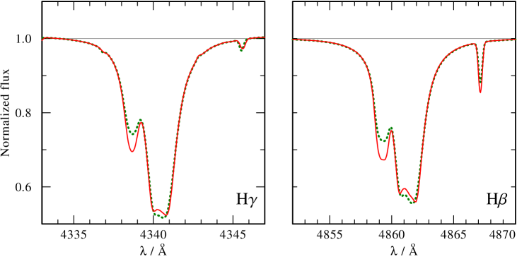
Figure 5: The H$\gamma$ and H$\beta$ lines (left and right panels, respectively), as obtained from models (b) and (c) (red solid and green dotted lines, respectively), both with an effective gravity of $\log g_{\text{eff}}=2.47$. Although the strengh of the line wings is the same, the two models imply masses and gravities, which strongly differ because of the different treatment of the radiative pressure (cf. Table 4)

3.3 Comparison with fixed $g_{\text{eff}}$

In the models (a) and (b) discussed above, we specify $g_{\text{grav}}$, $T_{\ast}$, and $L$, and therefore the radii, the spectroscopic masses are known a priori. When dealing with observations, however, it is $g_{\text{eff}}$, and not $g_{\text{grav}}$, which is empirically measurable. Thus, one would fix the effective gravity that best reproduces the observation, and let the actual gravity $g_{\text{grav}}$ be a model output. Based on the detailed physics implemented in the model atmosphere, the gravity $g_{\text{grav}}$ and the spectroscopic mass $M_{\ast}$ follow from $\log g_{\text{eff}}$. This scenario is reflected in models (b) and (c), which are calculated with identical effective gravities, but with a different treatment of the radiation pressure in the quasi-hydrostatic domain. Fig. 5 shows the Balmer lines H$\gamma$ (left panel) and H$\beta$ (right panel) as obtained from the supergiant models (b),, which account for $\Gamma_{\text{rad}}$ (red solid line), and (c), which only include $\Gamma_{\text{e}}$ (green dotted line). As both models have the same $g_{\text{eff}}$, the line wings obtained from both models can hardly be distinguished. However, some differences are seen in the line cores and in the helium and metal lines.

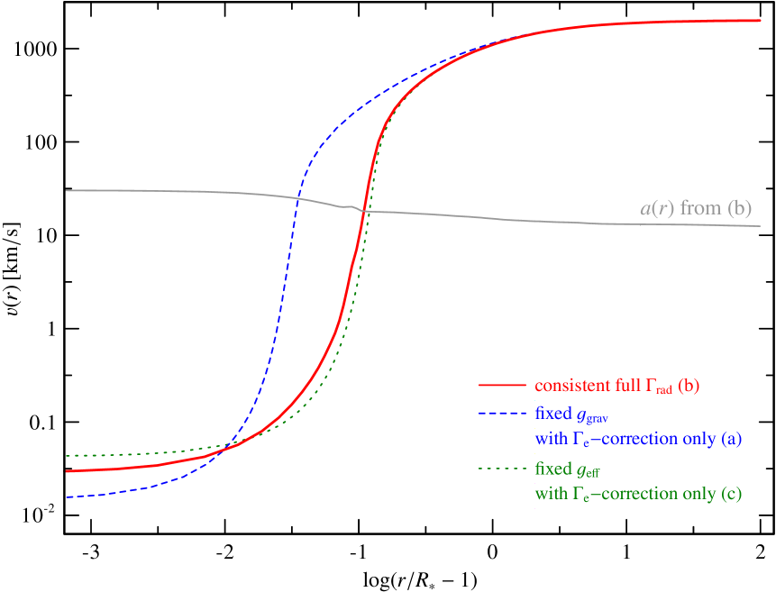
Figure 6: Velocity stratification for three supergiant test models: the consistent quasi-hydrostatic model (b) (red solid) is compared to a model (a) (blue dashed) with the same $g_{\text{grav}}$, but where only $\Gamma_{\text{e}}$ is taken into account in the quasi-hydrostatic part (blue). The third model (c) (green dotted) shares $g_{\text{eff}}$ with model (b), except it accounts only for $\Gamma_{\text{e}}$ and thus has a different $g_{\text{grav}}$.

To illustrate the effect of this different treatment, we show the velocity stratification for all three supergiant models in Fig. 6. All models agree in the outer part where we have prescribed the $\beta$-law. However, in the inner part it becomes evident that fixing $g_{\text{eff}}$ indeed leads to relatively similar velocity stratifications with both the consistent $\overline{\Gamma}_{\text{rad}}$-approach and the $\Gamma_{\text{e}}$-approach, which is reflected in the agreement of line profiles between the models (b) and (c). If one fixes instead the more fundamental parameter $g_{\text{grav}}$, the resulting velocity stratification is significantly different in the inner part, if accounting only for $\Gamma_{\text{e}}$, including a huge difference in the radial location of the sonic point. These discrepancies explain the spectral differences between models (a) and (b) shown in Fig. 4.

Table 4: Deduced stellar masses with different quasi-hydrostatic approaches

Luminosity class	I	III	V
$\log g_{\text{eff}}$ [cm s-2]	$2.47$	$3.02$	$3.79$
$\log g_{\text{grav}}(\Gamma_{\text{e}})$ [cm s-2]	$3.00$	$3.25$	$3.82$
$\log g_{\text{grav}}(\Gamma_{\text{rad}})$ [cm s-2]	$3.25$	$3.50$	$4.00$
$M_{\ast}(\Gamma_{\text{e}})$ [M⊙]	$14.5$	$12.9$	$16.2$
$M_{\ast}(\Gamma_{\text{rad}})$ [M⊙]	$25.9$	$23.0$	$24.1$

Despite the similarities between the models (b) and (c) seen in the line wings and in the velocity law, their values of $\log g_{\text{grav}}$ and $M_{\ast}$ differ significantly. Table 4 shows the values of $\log g_{\text{grav}}$ and $M_{\ast}$ for the dwarf, giant, and supergiant models. As could be anticipated from Eq. (30), the models that account for the full radiative pressure (models b) have larger values for $\log g_{\text{grav}}$ and $M_{\ast}$ because their $\Gamma,$ which is used to relate $g_{\text{eff}}$ and $g_{\text{grav}}$ , is larger in these models. The spectroscopic masses deviate by roughly a factor of two. Interestingly, there is no clear trend for increasing deviation with increasing luminosity class. Intuitively, one might expect that the deviation would have to be larger for the supergiant model, compared to the dwarf model, as we obtained it in spectral comparison of the models (a) and (b) which were shown in Fig. 4. However, the calculation of the (c) models is quantitatively different from the (a) models. Even though both consider only $\Gamma_{\text{e}}$ for obtaining the velocity field in the quasi-hydrostatic part, the (c) models are specifically designed to reproduce the $g_{\text{eff}}$-value obtained with the full $\Gamma_{\text{rad}}$ , while the (a) models have a completely different approach, with the $g_{\text{grav}}$-value being identical to the (b) models. In fact, we can estimate the masses of the (c) models with an easy calculation. Starting from the requirement that both, (b) and (c) models should have the same $g_{\text{eff}}$, it immediately follows via Eq. (28) that

$$M_{\ast}^{(c)}\left(1-\Gamma_{\text{e}}^{(c)}\right)=M_{\ast}^{(b)}\left(1-\overline{\Gamma}_{\text{rad}}^{(b)}\right)\text{.}$$ (32)

The small superscripts indicate the value from the corresponding model family, i.e., $M_{\ast}^{(c)}$ is short for $M_{\ast}(\Gamma_{\text{e}})$ in the (c) models. As we do not know $\Gamma_{\text{e}}^{(c)}$ in advance, since it contains $M_{\ast}(\Gamma_{\text{e}})$ itself by definition (22), we need to replace it with a value from the (b) model. Because the luminosity $L$ is the same in the (b) and the (c) models and the ionization parameter $q_{\text{ion}}$ only changes marginally, we can deduce from Eq. (22) that the product of $\Gamma_{\text{e}}$ and $M_{\ast}$ will be approximately the same for both models. Hence we get an expression that allows us to replace $\Gamma_{\text{e}}^{(c)}$ with the known $\Gamma_{\text{e}}^{(b)}$, i.e.,

$$\Gamma_{\text{e}}^{(c)}\approx\frac{M_{\ast}^{(b)}}{M_{\ast}^{(c)}}\Gamma_{\text{e}}^{(b)}.$$ (33)

Using that in (32) yields

$$M_{\ast}^{(c)}-M_{\ast}^{(b)}\Gamma_{\text{e}}^{(b)} \approx M_{\ast}^{(b)}\left(1-\overline{\Gamma}_{\text{rad}}^{(b)}\right)$$ (34)

$$M_{\ast}^{(c)} \approx M_{\ast}^{(b)}\left[1-\left(\overline{\Gamma}_{\text{rad}}^{(b)}-\Gamma_{\text{e}}^{(b)}\right)\right]\text{.}$$ (35)

This means that masses of the (c) models only depend on the difference between $\overline{\Gamma}_{\text{rad}}$ and $\Gamma_{\text{e}}$ in the consistent (b) models, not on the absolute values. The difference is comparable for all three luminosity classes, and so is the mass deviation in Table 4.

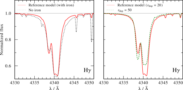
Figure 7: Left panel: the spectrum around H$\gamma$ for the hydrostatically consistent supergiant test model (red solid line) is compared to a similar PoWR model calculated without iron group elements (black dotted line). Right panel: the same test model is calculated with a higher Doppler broadening velocity $\varv_{\text{dop}}$ (green dashed line) and compared to the original.

3.4 Blanketing and Doppler velocity influence

It is unfortunate that the spectroscopic mass greatly depends on various parameters adopted in the calculation. Two important examples will be discussed here. The first is the importance of the iron group elements. Since they are a dominant source for opacity in the atmosphere of a massive star, their abundances significantly affect the radiative pressure, and thus the inferred spectroscopic mass. Therefore iron group elements have to be included in model atmosphere calculations, even if these models are only used to analyse spectral regimes without visible iron lines. The effect, which is called “line blanketing”, does not only affect the temperature stratification, but also the density structure of a stellar atmosphere. This is illustrated in left panel of Fig. 7, where we compare the H$\gamma$ line from our supergiant model (see Table 2 for parameters) to that of an identical model without iron. It impressively demonstrates that neglecting elements, which greatly contribute to the total opacity, is not legitimate. When the iron elements are not included, the radiative pressure is smaller, and the line wings appear broader in the synthetic spectrum, leading to an underestimation of the gravity by $\approx 0.3$ dex. These elements should thus be included in any consistent calculation, even if there is no observational abundance indicator. Using “typical” abundances from the local region or similar objects will usually cause a smaller error than neglecting such elements completely.

Another quantity that is of major influence on the spectral appearance of OB star atmosphere models is the adopted Doppler broadening velocity $\varv_{\text{dop}}$. This velocity is used in the comoving frame calculations and reflects the combined influence of the thermal and microturbulent velocities. While the thermal velocity is calculated for each element as a depth-dependent manner in the formal integral, the comoving frame calculations are currently using a constant $\varv_{\text{dop}}$ for all elements. For the spectral appearance of Wolf-Rayet atmospheres the value of $\varv_{\text{dop}}$ is of minor importance, but it has a notable impact on the spectra of our OB models, as it affects the total radiative pressure in the atmosphere. This is illustrated in the right panel of Fig. 7, where we again compare the region around H$\gamma$ for our supergiant test model, but now compare with a model that has been calculated with a larger Doppler velocity. In the O-star regime, the value of $\varv_{\text{dop}}=20\,$km/s has proved to be sufficient. This demonstrates that it is imperative to choose a $\varv_{\text{dop}}$ reflecting the true thermal and turbulent velocity in the stellar atmosphere, despite the significantly longer computing times in the comoving frame calculations that come along with smaller values of $\varv_{\text{dop}}$.

4 Comparison with TLUSTY

The TLUSTY code (Hubeny & Lanz 1995b) provides plane-parallel model atmospheres. The synthetic spectra that can be calculated from these models, e.g., with the SYNSPEC program from the same authors, are widely used for the analysis of photospheric spectra of OB-type stars. In the following section, we compare PoWR and TLUSTY model results. In all cases where spectra based on TLUSTY models are shown, they were obtained with the SYNSPEC code and are labeled as TLUSTY.

While both PoWR and TLUSTY are non-LTE codes, a major difference is that the PoWR models include the stellar wind. PoWR therefore adopts a spherical geometry, while TLUSTY assumes a plane-parallel geometry. As thoroughly discussed by Lanz & Hubeny (2003), the assumption of static, plane-parallel atmospheres is a fairly solid approximation for the photospheres of OB stars, which show negligible signs of stellar winds and curvature effects. One can therefore expect that in the limit of negligible mass-loss rates and small scale heights (see Eq. 4), the PoWR spectra would be close to the TLUSTY results. To check that PoWR models of OB-type stars with negligible winds show a good agreement with the corresponding TLUSTY models, we dedicate this section to a comparison of dwarf, giant, and supergiant PoWR models with their TLUSTY counterparts, focusing on the pressure-broadened Balmer lines. In all cases, PoWR models with the consistently treated quasi-hydrostatic domain are used, i.e., those models that we referred to as type (b) above.

Since we calcuated the models used in Sect. 3 with “typical” O-star mass-loss rates, they are not expected to provide a very close agreement with the TLUSTY models. The discrepancies are most prominent in the H$\alpha$ line for the supergiant and giant models, while small differences are also found in the other Balmer lines. In Fig. 8, we illustrate the effect of reducing the mass-loss rate. It is evident that the spectral appearance converges in the limit of small mass loss, and it is at this limit where we expect to obtain the closest agreement with TLUSTY models. Furthermore, the sequence of models illustrates that the absence of emission lines is not sufficient to deduce that mass loss is negligible.

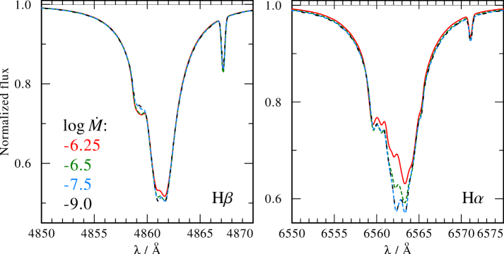
Figure 8: Profiles of the H$\alpha$ and H$\beta$ lines from PoWR models with different $\dot{M}$. In the limit of low mass-loss rates, the wind effect on the spectrum becomes negligible. For an easier comparison of the line wings, the electron redistribution (see Fig. 9) is switched off in these simulations.

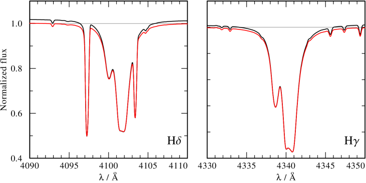
Figure 9: Line profiles of H$\gamma$ and H$\delta$ for the same supergiant PoWR model. The red line denotes the spectrum that is obtained when switching off the electron redistribution in the formal integral, while the black line indicates the “normal” output, which includes the redistribution of free electrons.

Another PoWR feature, which would hinder a comparison with the TLUSTY models, is frequency redistribution by Thomson scattering (Mihalas 1978). Given their large thermal velocities (${\sim}1000\,$km ${\rm s}^{-1}$), free electrons can scatter photons to significantly different wavelengths. Hence, photons that are trapped in an optically thick line core can be Doppler-shifted to the line wing or adjacent continuum, from which they can freely emerge and become visible as an excess emission. Especially at lower surface gravities and in spectral domains with a high density of spectral lines, the effect of frequency redistribution often results in a noticeable pseudocontinuum. When the synthetic flux is normalized relative to the continuum, this has the appearance of a continuum offset in the normalized spectrum. To illustrate this effect, Fig. 9 shows the H$\delta$ and H$\gamma$ lines (left and right panels, respectively) for the consistent supergiant model including frequency redistribution (black solid line) and without (red solid line). Since TLUSTY does not account for this effect, we disable it for the sake of comparison. However, we stress that the importance of this effect has been demonstrated in various studies (Hummer & Mihalas 1967; Auer & Mihalas 1968).

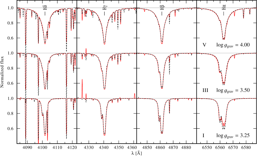
Figure 10: Balmer line comparison between the PoWR models (red, solid line) and the TLUSTY models (black, dashed line) for dwarfs (upper panels), giants (middle panels), and supergiants (lower panels). The stellar parameters used in the PoWR models are as in Table 2, but with negligible mass-loss rates ($\log\dot{M}=-9\,[M_{\odot}\,{\rm yr}^{-1}]$), small terminal velocities (500 km ${\rm s}^{-1}$), and large radii, to avoid wind and curvature effects.

The upper, middle, and bottom panels of Fig. 10 show a comparison between the TLUSTY (black, dashed line) and PoWR (red, solid line) for the dwarf, giant, and supergiant models, respectively, where we compare the first four Balmer members (from left to right: H$\delta$, H$\gamma$, H$\beta$, H$\alpha$). The PoWR model parameters are identical to those compiled in Table 2, but with a negligible mass-loss rate of $\log\dot{M}=-9.0$ $[M_{\odot}\,{\rm yr}^{-1}]$ and a small terminal velocity of $500\,$km ${\rm s}^{-1}$. Furthermore, the radii of all stars were set to large values to diminish possible curvature effects and to approach a plane-parallel geometry.

It is evident that a very good agreement in the line wings is obtained between the PoWR and TLUSTY models for all three luminosity classes. In particular, the wings of the Balmer lines are barely distinguishable. Hence, the application of either models would result in practically the same surface gravity, provided that the mass loss is really negligible. Interestingly, pressure broadening in the TLUSTY O-grid models from Lanz & Hubeny (2003) uses analytical approximations to numerical calculations (cf. Hubeny et al. 1994, appendix B), while PoWR performs interpolation over pressure broadening tables (Lemke 1997) for hydrogen lines. Given the good agreement, both methods seem to be adequate for the studied parameter regime, i.e., nondegenerated stars.

While a comprehensive comparison between PoWR and TLUSTY along all spectral lines is beyond the scope of the current paper, we note that there are significant differences regarding helium and metal lines. Not only does their strength differ by up to a factor of two between TLUSTY and PoWR, but sometimes – as visible in the supergiant comparison – they may even appear in emission from one code, and absorption from the other. Because of the non-LTE conditions, even small differences in the stratification can have large effects on such weak lines, e.g., between two PoWR models differing only slightly in their temperature or gravity. Indeed, we find similar discrepancies in the small lines. This can be seen in Fig. 4, where we compare the $\overline{\Gamma}_{\text{rad}}$- and $\Gamma_{\text{e}}$-model spectra. Therefore one has to be careful deducing parameters, e.g., abundances, from only one particular line. Instead, several lines of more than one ionization stage should be compared if available.

5 Summary and conclusions

We present a set of stellar atmosphere models calculated with the most recent version of the PoWR code, using different approaches for the quasi-hydrostatic regime. In the limit of small mass-loss rates, we also compared the PoWR models to the plane-parallel TLUSTY atmospheres.

We conclude that a proper treatment of the quasi-hydrostatic regime is imperative for OB-type star modeling. For a consistent solution, the full radiative acceleration has to be taken into account, including line and continuum contributions.

The spectroscopic masses will be severely underestimated, by a factor of roughly 2, if models are used that account only for the radiation pressure on free electrons in the quasi-hydrostatic domain. This holds for all luminosity classes.

Omitting elements that significantly contribute to the total opacity compromises the density stratification in the quasi-hydrostatic domain, and consequently leads to an inconsistent stellar masses. Specifically neglecting important elements, such as Fe, in the models is by no means legitimate.

The effect of mass loss on the spectra of typical OB stars may seem subtle, but even small mass-loss rates can change the line profile and thus might affect deduced gravities. The absence of emission lines in an observation does not imply negligible mass loss.

In the limit of small mass-loss rates and vanishing curvature effects, the emergent spectra of the PoWR model atmospheres generally agree very well with TLUSTY models calculated with the same stellar parameters.