Estimating the Probability of Meeting a
Deadline in Hierarchical Plans.

Abstract

Given a hierarchical plan (or schedule) with uncertain task times, we propose a deterministic polynomial (time and memory) algorithm for estimating the probability that its meets a deadline, or, alternately, that its makespan is less than a given duration. Approximation is needed as it is known that this problem is NP-hard even for sequential plans (just, a sum of random variables). In addition, we show two new complexity results: (1) Counting the number of events that do not cross deadline is #P-hard; (2) Computing the expected makespan of a hierarchical plan is NP-hard. For the proposed approximation algorithm, we establish formal approximation bounds and show that the time and memory complexities grow polynomially with the required accuracy, the number of nodes in the plan, and with the size of the support of the random variables that represent the durations of the primitive tasks. We examine these approximation bounds empirically and demonstrate, using task networks taken from the literature, how our scheme outperforms sampling techniques and exact computation in terms of accuracy and run-time. As the empirical data shows much better error bounds than guaranteed, we also suggest a method for tightening the bounds in some cases.

1 Introduction

Numerous planning tools produce plans that call for executing tasks non-linearly. Usually, such plans are represented as a tree, where the leaves indicate primitive tasks, and other nodes represent compound tasks consisting of executing their sub-tasks either in parallel (also called “concurrent” tasks [2]) or in sequence  [3, 4, 5, 6].

Given such a hierarchical plan representation, it is frequently of interest to evaluate its desirability in terms of resource consumption, such as fuel, cost, or time. The answer to such questions can be used to decide which of a set of plans, all valid as far as achieving the goal(s) are concerned, is better given a user-specified utility function. Another reason to compute these distributions is to support runtime monitoring of resources, generating alerts to the execution software or human operator if resource consumption in practice has a high probability of surpassing a given threshold.

While most tools aim at good average performance of the plan, in which case one may ignore the full distribution and consider only the expected resource consumption [7], our paper focuses on providing guarantees for the probability of meeting deadlines. This type of analysis is needed, e.g., in Service-Level-Agreements (SLA) where guarantees of the form: “response time less than 1mSec in at least 95% of the cases” are common [8], Section 10 discusses additional related work. We assume that a hierarchical plan is given in the form of a tree, with uncertain resource consumption of the primitive actions in the network, provided as a probability distribution. The problem is to compute a property of interest of the distribution for the entire task network. In this paper, we focus mainly on the issue of computing the probability $P(X_{\tau}\leq T)$ of satisfying a deadline $T$ where $X_{\tau}$ is a random variable describing the distribution of the makespan of the plan. Since in the above-mentioned applications for these computations, one needs results in real-time (for monitoring) or multiple such computations (in comparing candidate plans), efficient computation here is crucial, and is more important than in, e.g., off-line planning.

The decision problem we analyze is: given a task tree and a deadline, does the probability of meeting this deadline is above a given threshold. We show that this decision problem is NP-hard (see Section 7), the first contribution of this paper. We propose a deterministic polynomial-time approximation scheme for this problem, a second contribution of this paper. Error bounds are analyzed and are shown to be tight. For discrete random variables with finite support, finding the distribution of the maximum can be done in low-order polynomial time. However, when compounded with errors generated due to approximation in subtrees, handling this case requires careful analysis of the resulting error. The approximations developed for both sequence and parallel nodes are combined into an overall algorithm for task trees, with an analysis of the resulting error bounds, yielding a polynomial-time (additive error) approximation scheme for computing the probability of satisfying a deadline for the complete network, another contribution of this paper. We also consider computing expected makespan. Since for discrete random variables, in parallel nodes one can compute an exact distribution efficiently, it is easy to compute an expected makespan in this case as well as for sequence nodes. Despite that, we show that for trees with both parallel and sequence nodes, computing the expected makespan is hard.

Experiments are provided in order to examine the quality of approximation in practice when compared to the theoretical error bounds. A simple sampling scheme is also provided as a yardstick, even though the sampling does not come with error guarantees, but only bounds in probability. Finally, we examine our results in light of related work in the fields of planning and scheduling, as well as probabilistic reasoning.

2 Problem statement

We are given a hierarchical plan represented as a task tree consisting of three types of nodes: primitive actions as leaves, sequence nodes, and parallel nodes. Primitive action nodes contain distributions over their resource consumption. Many resources can be modeled using the proposed approach. For example if the resource of interest is memory, tasks running in parallel use the sum of the memory space of each of the tasks; if they run in sequence, only the maximum thereof is needed. Note that the role parallel and sequence node is inversed here. We will assume henceforth, in order to be more concrete, that the resource of interest is time, i.e., that parallel nodes represent maximum and sequence nodes represent sum.

The tasks trees that we analyze are composed of sequence nodes, parallel nodes and leaves that we call primitive tasks. A sequence node represents a composition of tasks in sequence. Its makespan is the the sum of the makespans of its child nodes. A parallel node represents a composition of tasks in parallel. Its makespan is the maximum of the makespan of its child nodes. The makespans of the primitive nodes at the leafs of the tree are uncertain, and described as probability distributions. We assume that the distributions are independent (but not necessarily identically distributed). We also assume initially that the random variables are discrete and have finite support (i.e. the number of values for which the probability is non-zero is finite). In this paper, we use the term $P_{X}$ to denote the (discrete) probability distribution of a (discrete) random variable $X$, i.e., the list of the probabilities of the outcomes, also known as the probability mass function. We use the term $F_{X}$ to denote the cumulative distribution function, i.e., $F_{X}(x)$ is the probability that $X$ will take a value less than or equal to $x$. More specifically, as the resource of interest is completion time, we associate each leaf node, $v$, with the random variable, $X_{v}$, that represents the distribution of the a completion-time distribution $P_{X_{v}}$ and a cumulative distribution function (CDF) $F_{X_{v}}$.

For clarity, we use the following standard for notations in the paper. First, we denote all random variables by symbols of the form $X_{name}$ where in the subscript we put the name of the variable. Second, we use the symbol $\tau_{name}$ where the subscript contains a name of a node to denote the subtree starting at this node, i.e., the node is the root of the subtree. Note that $X_{\tau_{v}}$ and $X_{v}$ have the same meaning - a random variable representing the makespan of the subtree $\tau_{v}$. Last, we use primed versions of random variables to denote approximations, i.e., the symbol $X^{\prime}_{name}$ denotes an approximation of the random variable $X_{name}$.

The main computational problem analyzed in this paper is the deadline problem:

Definition 1.

Given a task tree $\tau$ and a deadline $T$, the deadline problem is to compute $F_{X_{\tau}}(T)$.

In words, given a task tree $\tau$ and a deadline $T$, we ask what is the probability that the plan modeled by $\tau$ terminates in time less than $T$?

The above deadline problem reflects a step utility function: a constant positive utility $U$ for all $t$ less than or equal to a deadline time $T$, and $0$ for all $t>T$. We also briefly consider a linear utility function, requiring computation of the expected completion time of $\tau$, and show that this expectation problem is also NP-hard. The duration of a sequence node $s$ is a random variable:

$$X_{s}=\sum_{c\in\operatorname{\operatorname{children}}(s)}X_{c}$$

where $X_{c}$ is a random variable representing the duration of the plan modeled by the subtree rooted at the child node $c$ and $\operatorname{\operatorname{children}}(s)$ is the set of children of $s$.

Likewise, the duration distribution of a parallel node $p$ is a random variable:

$$X_{p}=\max_{c\in\operatorname{\operatorname{children}}(p)}X_{c}$$

Let $r$ be the root node of a task tree $\tau$ and $X_{r}$ be a random variable representing the duration distribution of the root. Then the probability that the plan meets the deadline $T$ is $F_{X_{r}}(T)$. Thus we need to compute the CDF, which is NP-hard [9]. We show how to deterministically approximate the CDF of the root with additive error at most $\varepsilon$ in time polynomial in $1/\varepsilon$.

Figure 1 is a simple hierarchical plan example. The set of nodes $V$ represented by $\{A,B,C,a,b,c,d,e\}$ and the type of each task node implied by its shape, $A$ and $C$ are sequence nodes, $B$ is a parallel node, and $a,b,c,d,e$ are all primitive nodes. Every primitive node is associated with probability mass function (PMF) describes the completion-time distribution. In this case $P_{X_{a}}(x)=P_{X_{b}}(x)=P_{X_{c}}(x)=P_{X_{d}}(x)=P_{X_{e}}(x)$.

$$P_{X_{a}}(x)=\begin{cases}1/4&\text{if }x=1;\\ 3/4&\text{if }x=4;\\ 0&otherwise.\end{cases}$$

This tree gives execution instructions: run $a$ and $b$ in parallel, then run $c$ and $d$ in sequence and, when they finish, run $e$.

Figure 1: Example of a hierarchical plan and its graphical representation.

Example 1.

Given a task tree $\tau$ as in figure  1, we will compute the duration distribution in the form of PMF for each compound task node including the root node, and then we will return the probability for $\tau$ to satisfy a given deadline $T$. First, compute duration distribution for the node $B$. The children task nodes $a,b$, are executed in parallel, therefore we need to find the distribution over the maximum of nodes $a$ and $b$:

$$P_{X_{B}}(x)=P_{\max(X_{a},X_{b})}(x)=\begin{cases}1/16&\text{if }x=1;\\ 15/16&\text{if }x=4;\\ 0&otherwise.\end{cases}$$

Second, compute duration distribution for node $C$. The children task nodes $c,d$, are executed in sequence, therefore, we need to use convolution in order to compute the sum of duration distributions of nodes $c$ and $d$:

$$P_{X_{C}}(x)=P_{X_{c}+X_{d}}(x)=\begin{cases}1/16&\text{if }x=2;\\ 3/8&\text{if }x=5;\\ 9/16&\text{if }x=8;\\ 0&otherwise.\end{cases}$$

Last, compute duration distribution for node $A$, the root node. The children task nodes $B,C,e$ are executed in sequence, therefore, we need to use convolution in order to compute the sum of duration distributions of nodes $B$, $C$ and $e$:

$$P_{X_{\tau}}=P_{X_{A}}(x)=P_{X_{B}+X_{C}+X_{e}}(x)=\begin{cases}1/1024&\text{if }x=4;\\ 3/128&\text{if }x=7;\\ 81/512&\text{if }x=10;\\ 27/64&\text{if }x=13;\\ 405/1024&\text{if }x=16;\\ 0&otherwise.\end{cases}$$

For every deadline $T$ we can easily return the probability for $\tau$ to satisfy $T$. If $T=8$, the probability is $F_{X_{\tau}}(8)=25/1024$ .

3 Sum (sequence) nodes

The size of the support (number of non-zero probability values) of the sum of random variables may be exponential in the number of variables, even for 2-valued variables. In fact, as shown in [9], computing the CDF of a sum of random variables at a given point is NP-hard. We thus define a notion of approximation, which we call a Kolmogorov upper bound (defined below), and supply an operator, we call $\operatorname{Trim}$, that produces such an approximation.

Let $X$ and $X^{\prime}$ be random variables; the Kolmogorov distance [10] between $X$ and $X^{\prime}$ is defined as:

$$d_{K}(X,X^{\prime})=\sup_{x}|F_{X^{\prime}}(x)-F_{X}(x)|$$

Our notion of approximation uses the Kolmogorov distance. Let $0\leq\varepsilon<1$. If the following equation holds:

$$\forall~{}x,~{}F_{X}(x)+\varepsilon\geq F_{X^{\prime}}(x)\geq F_{X}(x)$$

we say that the random variable $X^{\prime}$ is a Kolmogorov $\varepsilon$ upper bound approximation of $X$, which we denote by $X^{\prime}\succeq_{\varepsilon}X$. Contrapositively, we call $X$ a Kolmogorov $\varepsilon$ lower bound approximation of $X^{\prime}$. Note that $X^{\prime}\succeq_{\varepsilon}X$ implies that $d_{K}(X,X^{\prime})\leq\varepsilon$, but not vice-versa.

In our algorithms and examples, the PMF of a random variable $X$ is represented by a list $D_{X}$, which consists of $d=(p,x)$ pairs, where $x\in\operatorname{support}(X)$ and $p$ is the probability $P(X=x)$. In the pair $d=(p,x)$, we denote the value $x$ by $val(d)$, and the probability $p$ by $prob(d)$. For example, let $X$ be a random variable distributed as: $[0.1:1,0.1:2,0.8:4]$, and $X^{\prime}$ a random variable distributed as $[0.2:1,0.8:4]$. Then we have $X^{\prime}\succeq_{0.1}X$. In order to achieve a Kolmogorov upper bound of $\varepsilon$, the $\operatorname{Trim}_{U}$ operator removes consecutive domain values whose accumulated probability is less than $\varepsilon$ and adds their probability mass to the element in the support that precedes them.

If the input $D_{X}$ to $\operatorname{Trim}$ is sorted in increasing order of $x$ (we denote this operator by $\operatorname{Trim}_{U}(X,\varepsilon)$) then resulting variable $X^{\prime}$ (represented by the output $D_{X^{\prime}}$) is a Kolmogorov $\varepsilon$ upper bound of $X$. Likewise, if $D_{X}$ sorted in decreasing order of $x$ (in this case we denote the $\operatorname{Trim}$ operator by $\operatorname{Trim}_{L}(X,\varepsilon)$) then $X^{\prime}$ is a Kolmogorov $\varepsilon$ lower bound of $X$.

From now on, in order to simplify, we will use the notation $\operatorname{Trim}$ instead of $\operatorname{Trim}_{U}$. Note that we could have chosen to use $\operatorname{Trim}_{L}$ instead and get a symmetric version of all the results.

1 $D_{X^{\prime}}=()$, $p=0$

2 $d_{prev}=first(D_{X})$

3 $tail=rest(D_{X})$

4 while not-empty($tail$) do

5       $d=first(tail)$

6       if $p+prob(d)\leq\varepsilon$ then

7             $p=p+prob(d)$

8            

9      else

10             Append $(val(d_{prev}),prob(d_{prev})+p)$ to $D_{X^{\prime}}$

11             $d_{prev}=d$, $p=0$

12            

13      $tail=rest(tail)$

14Append $(val(d_{prev}),prob(d_{prev})+p)$ to $D_{X^{\prime}}$

15 return $D_{X^{\prime}}$

Algorithm 1 $\operatorname{Trim}$($D_{X}$,$\varepsilon$)

Trimming decreases the support size, while introducing an error. The trick is to keep the support size under control, while making sure that the error does not increase beyond a desired tolerance. Note that the size of the support can also be decreased by simple “binning” schemes, but these may not provide the desired guarantees.

We now show that with $D_{X}$ sorted in a increasing order, $\operatorname{Trim}(D_{X},\varepsilon)$ is an Kolmogorov $\varepsilon$ upper bound of $X$.

Lemma 1.

$\operatorname{Trim}(X,\varepsilon)\succeq_{\varepsilon}X$

Proof.

Let $X^{\prime}=\operatorname{Trim}(X,\varepsilon)$. Let $x_{1}{<}\cdots{<}x_{m}$ be the support of $X^{\prime}$. Because $\operatorname{Trim}$ adds the probabilities of elements that were removed from the support of $X$ to the support element of $X^{\prime}$ that precedes them, we have for all $i$:

$$P_{X^{\prime}}(x_{i})=P_{X}(x_{i})+P(x_{i}<X<x_{i+1})$$ (1)

(assuming $x_{m+1}=\infty$ for convenience.) The value $P(x_{i}<X<x_{i+1})$ equals the value of $p$ in the algorithm when the Append is performed, and the loop invariant $0\leq p\leq\varepsilon$ holds by construction. For any value $x$, let $l_{x}=\max\{i\colon x_{i}\leq x\}$, thus:

$$F_{X^{\prime}}(x)=\sum_{i=0}^{l_{x}}P_{X^{\prime}}(x_{i})$$

From Equation (1) we get:

$$F_{X^{\prime}}(x)-F_{X}(x)$$

$${=}\sum_{i=0}^{l_{x}-1}(P_{X^{\prime}}(x_{i})-P(x_{i}\leq X<x_{i+1}))+(P_{X^{\prime}}(x_{l_{x}})-P(x_{l_{x}}\leq X\leq x))$$

$${=}P_{X^{\prime}}(x_{l_{x}}){-}(P(x_{l_{x}}{\leq}X{<}x_{l_{x}+1}){-}P(x{<}X{<}x_{l_{x}+1}))$$

$${=}P(x<X<x_{l_{x}+1})\in(0,\varepsilon]$$

∎

Showing that $X\succeq_{\varepsilon}\operatorname{Trim}_{L}(X,\varepsilon)$, i.e. that using inversely sorted $D_{X}$ results in a Kolmogorov $\varepsilon$ lower bound, is immediate due to symmetry.

To bound the amount of memory needed for our approximation algorithm, the next lemma bounds the size of the support of the trimmed random variable:

Lemma 2.

$|\operatorname{support}(\operatorname{Trim}(D_{X},\varepsilon))|\leq 1/\varepsilon+1$

Proof.

In the Trim operator, each “Append” adds 1 to the support of $X^{\prime}$, and these occur only once inside the “else” statement, and once outside the loop. The “else” part of the loop occurs only if $p+prob(d)>\varepsilon$, after which none of these elements of the list are reused in the “if” statement. Therefore, as the sum of probabilities is 1, then the number of times the “else” part is executed is at most ${1}/{\varepsilon}$. Thus the total support is at most ${1}/{\varepsilon}+1$. ∎

The makespan of a $\operatorname{Sequence}$ operator is a random variable $X$, the sum of the random variables $X_{i}$ of its children. Let $Y_{i}=X_{i}+Y_{i-1}$ for $1<i\leq n$, and $Y_{1}=X_{1}$. Thus $X$ is distributed as $Y_{n}$.

As the children of a sequence node may be internal nodes in the task tree, the input distributions may already be approximations. To keep the size of the support small, we apply Trim after the addition of each random variable, i.e., we compute the random variables $Y^{\prime}_{i}=\operatorname{Trim}(X^{\prime}_{i}+Y^{\prime}_{i-1},\varepsilon)$, where the $X^{\prime}_{i}$ is a Kolmogorov $\varepsilon_{i}$ upper bound of $X_{i}$ and show that $Y^{\prime}_{n}$ is a Kolmogorov $\delta$ upper bound of $X$, for an appropriate $\delta$.

The distribution of the sum of random variables $X^{\prime}_{i}+Y^{\prime}_{i-1}$ is computed by a discrete convolution, and Trim is computed as in Algorithm 1. That is, our approximation for a $\operatorname{Sequence}$ operator (for $n\geq 2$) is given by:

$$\operatorname{Sequence}(X^{\prime}_{1},\dots,X^{\prime}_{n},\varepsilon)=\operatorname{Trim}(\operatorname{Convolve}(X^{\prime}_{1},\operatorname{Sequence}(X^{\prime}_{2},\dots,X^{\prime}_{n},\varepsilon)),\varepsilon)$$ (2)

We begin by bounding the approximation error propagated by convolution (sum of random variables ):

Lemma 3.

For discrete random variables $X_{1},X_{1}^{\prime},X_{2},X_{2}^{\prime}$ and $\varepsilon_{1},\varepsilon_{2}\in[0,1]$, if $X_{1}^{\prime}\succeq_{\varepsilon_{1}}X_{1}$ and $X_{2}^{\prime}\succeq_{\varepsilon_{2}}X_{2}$, then $X_{1}^{\prime}+X_{2}^{\prime}\succeq_{\varepsilon_{1}+\varepsilon_{2}}X_{1}+X_{2}$.

Proof.

Define error functions $E_{1}$ and $E_{2}$ such that $F_{X_{i}^{\prime}}(x)=F_{X_{i}}(x)+E_{i}(x)$. By construction, we have $0\leq E_{i}(x)\leq\varepsilon_{i}$.

By definition of sums of random variables and convolution, we have:

$$F_{X_{1}^{\prime}+X_{2}^{\prime}}(y)=\sum_{x=-\infty}^{\infty}F_{X_{1}^{\prime}}(y-x)P_{X_{2}^{\prime}}(x)$$

$$=\sum_{x=-\infty}^{\infty}(F_{X_{1}}(y-x)+E_{1}(y-x))P_{X_{2}^{\prime}}(x)$$

$$=\sum_{x=-\infty}^{\infty}F_{X_{1}}(y-x)P_{X_{2}^{\prime}}(x)+\sum_{x=-\infty}^{\infty}E_{1}(y-x)P_{X_{2}^{\prime}}(x)$$

$$\leq\sum_{x=-\infty}^{\infty}F_{X_{1}}(y-x)P_{X_{2}^{\prime}}(x)+\varepsilon_{1}\sum_{x=-\infty}^{\infty}P_{X_{2}^{\prime}}(x)$$

$$=\underbrace{\sum_{x=-\infty}^{\infty}F_{X_{2}^{\prime}}(y-x)P_{X_{1}}(x)}_{F_{X_{1}+X_{2}^{\prime}}(x)=F_{X_{2}^{\prime}+X_{1}}(x)}+\varepsilon_{1}\sum_{x=-\infty}^{\infty}P_{X_{2}^{\prime}}(x)$$

$$=\sum_{x=-\infty}^{\infty}(F_{X_{2}}(y-x)+E_{2}(y-x))P_{X_{1}}(x)+\varepsilon_{1}$$

$$=\sum_{x=-\infty}^{\infty}F_{X_{2}}(y-x)P_{X_{1}}(x)+\sum_{x=-\infty}^{\infty}E_{2}(y-x)P_{X_{1}}(x)+\varepsilon_{1}$$

$$\leq\sum_{x=-\infty}^{\infty}F_{X_{2}}(y-x)P_{X_{1}}(x)+\varepsilon_{2}\sum_{x=-\infty}^{\infty}P_{X_{1}}(x)+\varepsilon_{1}$$

$$\leq F_{X_{1}+X_{2}}(y)+\varepsilon_{2}+\varepsilon_{1}$$

Since $E_{i}(y)$ are non-negative, we also get $F_{X_{1}^{\prime}+X_{2}^{\prime}}(y)\geq F_{X_{1}+X_{2}}(y)$ for all $y$. ∎

The fact that this trade-off is linear allows us to get a linear approximation error in polynomial time, as shown below:

Theorem 1.

If $X_{i}^{\prime}\succeq_{\varepsilon_{i}}X_{i}$ for all $i\in\{1,\dots,n\}$ and $\hat{X}=\operatorname{Sequence}(X_{1}^{\prime},\dots,X_{n}^{\prime},\varepsilon)$ then $\hat{X}\succeq_{e}\sum_{i=1}^{n}X_{i}$, where $e={\sum_{i=1}^{n}\varepsilon_{i}+n\varepsilon}$.

Proof.

For $n$ iterations, from Lemma 3, we get an accumulated error of $\varepsilon_{1}+\dots+\varepsilon_{n}$. From Lemma 1, we get an additional error of at most $n\varepsilon$ due to trimming. ∎

Theorem 2.

Assuming that $m\leq 1/\varepsilon$, the procedure $\operatorname{Sequence}(X_{1}^{\prime},\dots,X_{n}^{\prime},\varepsilon)$ can be computed in time $O((nm/\varepsilon)\log(m/\varepsilon))$ using $O(m/\varepsilon)$ memory, where $m$ is the size of the largest support of any of the $X^{\prime}_{i}$s.

Proof.

From Lemma 2, the size of list $D$ in Algorithm 1 is at most $m/\varepsilon$ just after the convolution, after which it is trimmed, so the space complexity is $O(m/\varepsilon)$. $\operatorname{Convolve}$ thus takes time of $O((m/\varepsilon)\log(m/\varepsilon))$, where the logarithmic factor is required internally for sorting. Since the runtime of the $\operatorname{Trim}$ operator is linear, and the outer loop iterates $n$ times, the overall run-time of the algorithm is $O((nm/\varepsilon)\log(m/\varepsilon))$. ∎

The following example shows that our error bound is tight, that is, a sequence of random variables where the error actually achieves the bounds.

Example 2.

Let $0{\leq}\varepsilon{<}1$ and $n{\in}\mathbb{N}$ such that $1{-}\varepsilon{>}{\varepsilon}/{n}$, i.e., $\varepsilon$ is small or $n$ is large. Consider, for $\delta>0$ that we will choose to be very small, the random variable $X_{1}$ defined by

$$P_{X_{1}}(x){=}\begin{cases}\delta&\text{if }x=0,\\ {\varepsilon}/{(n(1-\delta)^{x})}&\text{if }x\in\{1,\dots,n\},\\ 1{-}\delta{-}\sum_{x=1}^{n}\frac{\varepsilon}{n(1-\delta)^{x}}&\text{if }x=n+1,\\ 0&\text{otherwise}\end{cases}$$

and, for $i\in\{2,\dots,n\}$, let the random variables $X_{i}$ be:

$$P_{X_{i}}(x)=\begin{cases}1-\delta&\text{if }x=0,\\ \delta&\text{if }x=n^{2},\\ 0&\text{otherwise}\end{cases}$$

The distribution of $X=X_{1}+X_{2}$ is

$$P_{X}(x){=}\begin{cases}\delta(1-\delta)&\text{if }x=0,\\ {\varepsilon}/{n}&\text{if }x=1,\\ {\varepsilon}/{(n(1-\delta)^{x-1})}&\text{if }x\in\{2,\dots,n\},\\ (1{-}\delta)P(X_{1}{=}n{+}1)&\text{if }x=n+1,\\ \delta P(X_{1}{=}x{-}n^{2})&n^{2}{\leq}x{\leq}n^{2}{+}n{+}1\\ 0&\text{otherwise}\end{cases}$$

The idea here is that the convolution with $X_{2}$ results in a random variable that is similar in “shape” to $X_{1}$, if we ignore numbers that tend to zero as $\delta$ approaches zero. The convolution also modifies the probability $P_{X}1)$ from slightly greater than $\varepsilon/n$ to precisely $\varepsilon/n$, which will then allow it to be trimmed.

Then, if we apply $\operatorname{Trim}(X_{1}+X_{2},\varepsilon/n)$, when $\delta$ is sufficiently small, we get the random variable $X^{\prime}$ whose probability distribution is:

$$P_{X^{\prime}}(x){=}\begin{cases}\delta(1-\delta)+{\varepsilon}/{n}&\text{if }x=0,\\ {\varepsilon}/{(n(1-\delta)^{x-1})}&\text{if }x\in\{2,\dots,n\},\\ 1-P(X^{\prime}{<}n+1)&\text{if }x=n+1,\\ 0&\text{otherwise.}\end{cases}$$

Note that indeed trimming shifts the mass from $P_{X}(1)=\varepsilon/n$ to $P_{X^{\prime}}(0)$. This repeats in all steps so, after $n$ steps, we get a random variable $X^{\prime}$ such that $P_{X^{\prime}}(0)\xrightarrow{\,\,\delta\to 0\,\,}\varepsilon$. Therefore, $P_{\operatorname{Sequence}(X_{1},\dots,X_{n},\varepsilon/n)}(0){-}P_{X_{1}{+}\dots+X_{n}}(0)$ approaches $\varepsilon$ as $\delta$ approaches zero which means that there exists no $\varepsilon^{\prime}{<}\varepsilon$ such that $\operatorname{Sequence}(X_{1},\dots,X_{n},\varepsilon/n)\succeq_{\varepsilon^{\prime}}X_{1}+\cdots+X_{n}$ for all $\delta>0$.

Observe that if we replace all upper Kolmogorov bound approximations by lower Kolmogorov bound approximations, all the results in this section still hold. Therefore, to obtain lower Kolmogorov bounds all that must be done is to repeat the computations using $\operatorname{Trim}_{L}$, that is, keeping the distribution representation sorted in reverse order.

4 Parallel nodes

Unlike sequence composition, the deadline problem for parallel composition is easy to compute, since the execution time of a parallel composition is the maximum of the durations:

$$F_{\max_{i\in[1:n]}X_{i}}(T){=}F_{\bigwedge_{i=1}^{n}X_{i}}(T){=}\prod_{i=1}^{n}F_{X_{i}}(T)$$ (3)

where the last equality follows from independence of the random variables. We denote the construction of the CDF using Equation (3) by $\textnormal{{Parallel}}(X_{1},\dots,X_{n})$. If the random variables are all discrete with finite support, $\textnormal{{Parallel}}(X_{1},\dots,X_{n})$ incurs linear space, and computation time $O(nmlog(n))$.

If the task tree consists only of parallel nodes, one can compute the exact CDF, with the same overall runtime. However, when the task tree contain both sequence and parallel nodes we may get only approximate CDFs as input, and now the above straightforward computation can compound the errors. When the input CDFs are themselves approximations, we bound the resulting error:

Lemma 4.

For discrete random variables $X_{1}^{\prime},\dots X_{n}^{\prime}$, $X_{1},\dots,X_{n}$, if for all $i=1,\dots,n$, $X_{i}^{\prime}\succeq_{\varepsilon_{i}}X_{i}$ and $0\leq\varepsilon_{i}\leq\frac{1}{n(Kn+1)}$ for some $K>0$, then, for any $\varepsilon\geq\varepsilon_{i}$, we have: $\max_{i\in[1:n]}X_{i}^{\prime}\succeq_{e}\max_{i\in[1:n]}X_{i}$ where $e=\sum_{i=1}^{n}\varepsilon_{i}+\varepsilon/K$.

Proof.

$F_{\max_{i\in[1:n]}X^{\prime}_{i}}(T){-}F_{\max_{i\in[1:n]}X_{i}}(T)$

$$\leq\prod_{i=1}^{n}(F_{X_{i}}(T)+\varepsilon_{i}){-}\prod_{i=1}^{n}F_{X_{i}}(T)$$

$$\leq\prod_{i=1}^{n}(1+\varepsilon_{i})-1\leq 1+\sum_{i=1}^{n}\varepsilon_{i}+\sum_{k=2}^{n}{n\choose k}\varepsilon^{k}-1$$

$$\leq\sum_{i=1}^{n}\varepsilon_{i}+\!\!\!\!\underbrace{\sum_{k=2}^{n}n^{k}\varepsilon^{k}}_{\text{sum of a geo. series}}\!\!\!\!\leq\sum_{i=1}^{n}\varepsilon_{i}+\frac{n^{2}\varepsilon^{2}}{1-n\varepsilon}\leq\sum_{i=1}^{n}\varepsilon_{i}+\varepsilon/K$$

Since $F_{X_{i}^{\prime}}(T)>F_{X_{i}}(T)$ for each $i$, this expression is nonnegative. ∎

Both in Lemma 4 and in Lemma 5 we suggest an upper bound of the error resulted in the case where the input CDFs themselves are approximations. However, Lemma 4 is designed to facilitate the proof of Theorem 4 and Lemma 4 is designed to facilitate the proof Theorem 5.

Lemma 5.

For discrete random variables $X_{1}^{\prime},\dots X_{n}^{\prime}$, $X_{1},\dots,X_{n}$, if for all $i=1,\dots,n$, $X_{i}^{\prime}\succeq_{\varepsilon_{i}}X_{i}$, then $\max\{X_{1}^{\prime},\dots,X_{n}^{\prime}\}\succeq_{e}\max\{X_{1},\dots,X_{n}\}$ where $e=1-\prod_{i=1}^{n}(1-\varepsilon_{i})$.

Proof.

When $F_{X^{\prime}}(T)>0$, we can write:

$$P(\max\{X_{1}^{\prime},\dots,X_{n}^{\prime}\}{\leq}T)-P(\max\{X_{1},\dots,X_{n}\}{\leq}T)$$

$$=\prod_{i=1}^{n}F_{X_{i}^{\prime}}(T)-\prod_{i=1}^{n}F_{X_{i}}(T)$$

$$=\prod_{i=2}^{n}F_{X_{i}^{\prime}}(T)(F_{X_{1}^{\prime}}(T)-F_{X_{1}}(T)\prod_{i=2}^{n}\frac{F_{X_{i}}(T)}{F_{X_{i}}(T)})$$

$$\leq\prod_{i=2}^{n}F_{X_{i}^{\prime}}(T)(F_{X_{1}^{\prime}}(T)-(F_{X_{1}^{\prime}}(T)-\varepsilon_{1})\prod_{i=2}^{n}\frac{F_{X_{i}}(T)}{F_{X_{i}}(T)})$$

$$\leq\prod_{i=2}^{n}F_{X_{i}^{\prime}}(T)(1-(1-\varepsilon_{1})\prod_{i=2}^{n}\frac{F_{X_{i}}(T)}{F_{X_{i}}(T)})$$

where the first inequality holds because $F_{X_{1}}(T)\leq F_{X_{1}^{\prime}}(T)-\varepsilon_{1}$, and the second inequality holds because $1\geq F_{X_{1}}(T)>0$ and the second product is positive and not greater than 1. Since we also have that $F_{X_{i}^{\prime}}(T)-F_{X_{i}}(T)\geq\varepsilon_{i}\geq 0$ for every $i$, these steps can be repeated, for $n\geq i\geq 2$, to get the expression: $1-\prod_{i=1}^{n}(1-\varepsilon_{i})$ as claimed. Due to monotonicity of max, we also have $F_{X^{\prime}}(T)-F_{X}(T)\geq 0$, which completes the proof. ∎

Example 3.

Let $0{\leq}\varepsilon{<}1$, the random variable $X$ defined by

$$P_{X}(x)=\begin{cases}1-\varepsilon&\text{if }x=0,\\ \varepsilon&\text{if }x=1,\\ 0&\text{otherwise}\end{cases}$$

The ”trimmed” version of $X$ in respect to $\varepsilon$, denoted by $X^{\prime}$, is:

$$P_{X^{\prime}}(x)=\begin{cases}1&\text{if }x=0,\\ 0&\text{otherwise}\end{cases}$$

Let $X_{1},\dots,X_{n}$ be $n$ independent copies of $X_{1}$ and let $X^{\prime}_{1},\dots,X^{\prime}_{n}$ be their “trimmed versions”. Then:

$$F_{\max\{X_{1}^{\prime},\dots,X_{n}^{\prime}\}}(0)-F_{\max\{X_{1},\dots,X_{n}\}}(0)$$

$$=\prod_{i=1}^{n}(1)-\prod_{i=1}^{n}(1-\varepsilon)=1-\prod_{i=1}^{n}(1-\varepsilon)$$

If we consider now a task tree with a single parallel aggregation level whose children are $n$ sequence nodes where the $i$th sequence node has a single primitive-task child modeled by $X_{i}$, we get that our computation will introduce exactly the higher bound predicted by Lemma 5, i.e, this bound is tight.

5 Task trees: mixed sequence/parallel

Given a task tree $\tau$ and a accuracy requirement $0<\varepsilon<1$, we generate a distribution for a random variable $X_{\tau}^{\prime}$ approximating the true duration distribution $X_{\tau}$ for the task tree. We introduce the algorithm and prove that the algorithm indeed returns an $\varepsilon$-approximation of the completion time of the plan. For a node $v$, let $\tau_{v}$ be the sub tree with $v$ as root and let $\operatorname{\operatorname{children}}(v)$ be the set of children of $v$. We use the notation $|\tau|$ to denote the total number of nodes in $\tau$.

1

2

3Let $v$ be the root of $\tau$ // Hence, $\tau_{v}=\tau$

4 $n_{v}=|\operatorname{\operatorname{children}}(v)|$

5 if $v$ is a $\operatorname{Primitive}$ node then

6       return the distribution of $v$

7      

8

9if $v$ is a $\operatorname{Sequence}$ node then

10       for $c\in\operatorname{\operatorname{children}}(v)$ do

11             $X^{\prime}_{c}$ = Network ($\tau_{c}$, $\frac{|\tau_{c}|\varepsilon}{|\tau_{v}|}$)

12            

13      return Sequence ($\{X^{\prime}_{c}\}_{c\in\operatorname{\operatorname{children}}(v)}$, $\frac{\varepsilon}{n_{v}|\tau_{v}|}$)

14

15if $v$ is a $\operatorname{Parallel}$ node then

16       for $c\in\operatorname{\operatorname{children}}(v)$ do

17             $X^{\prime}_{c}$ = Network ($\tau_{c}$, $\min(\frac{|\tau_{c}|\varepsilon}{|\tau_{v}|},\frac{1}{n_{v}(|\tau_{v}|n_{v}+1)})$)

18            

19      return Parallel ($\{X^{\prime}_{c}\}_{c\in\operatorname{\operatorname{children}}(v)}$)

20

21

Algorithm 2 Network($\tau$, $\varepsilon$)

Algorithm 2, that implements the operator Network, is a straightforward postorder traversal of the task tree. The only remaining issue is handling the error, in an amortized approach, as seen in the proof of the following theorem.

Theorem 3.

Given a task tree $\tau$, let $X_{\tau}$ be a random variable representing the true distribution of the completion time for the network. Then $\textnormal{{Network}}(\tau,\varepsilon)\succeq_{\varepsilon}X_{\tau}$.

Proof.

By induction on $|\tau|$. Base: $|\tau|=1$, the node must be primitive, and Network will just return the distribution unchanged which is obviously an $\varepsilon$-approximation of itself. Suppose the claim is true for $1\leq|\tau|<n$. Let $\tau$ be a task tree of size $n$ and let $v$ be the root of $\tau$. If $v$ is a $\operatorname{Sequence}$ node, by the induction hypothesis that $X^{\prime}_{c}\succeq_{|\tau_{c}|\varepsilon/|\tau_{v}|}X_{c}$, and by Theorem 1, the maximum accumulated error is $\sum_{c\in\operatorname{\operatorname{children}}(v)}{|\tau_{c}|\varepsilon}/|\tau_{v}|+{\varepsilon}/|\tau_{v}|$ = $(n-1)\varepsilon/|\tau_{v}|+{\varepsilon}/|\tau_{v}|=\varepsilon$ for $v$, therefore, $\textnormal{{Sequence}}(\{X^{\prime}_{c}\}_{c\in\operatorname{\operatorname{children}}(v)},{\varepsilon}/{n})\succeq_{\varepsilon}X_{\tau}$ as required. If $v$ is a $\operatorname{Parallel}$ node, by the induction hypothesis that $X^{\prime}_{c}\succeq_{e_{c}}X_{c}$, where $e_{c}=\min(\frac{|\tau_{c}|\varepsilon}{|\tau_{v}|},\frac{1}{n_{v}(|\tau_{v}|n_{v}+1)})$.

So $\sum_{c\in\operatorname{\operatorname{children}}(v)}e_{c}\leq\sum_{c\in\operatorname{\operatorname{children}}(v)}\frac{|\tau_{c}|\varepsilon}{|\tau_{v}|}\leq\varepsilon-\varepsilon/|\tau_{v}|$. Then, by Lemma 4, using $K=|\tau_{v}|$ and $n=n_{v}$, we get that $\textnormal{{Parallel}}(\{X^{\prime}_{c}\}_{c\in\operatorname{\operatorname{children}}(v)})\succeq_{\varepsilon}X_{\tau}$ as required. ∎

Theorem 4.

Let $N$ be the size of the task tree $\tau$, and $M$ the size of the maximal support of each of the primitive tasks. If $0\leq\varepsilon\leq\frac{1}{N(N^{2}+1)}$ and $M<N/\varepsilon$, the Network approximation algorithm runs in time $O((N^{5}/\varepsilon^{2})\log(N^{3}/\varepsilon^{2}))$, using $O(N^{3}/\varepsilon^{2})$ memory.

Proof.

The run-time and space bounds can be derived from the bounds on Sequence and on Parallel, as follows. In the Network algorithm, the trim accuracy parameter is less than or equal to ${\varepsilon}/{N}$. The support size (called $m$ in Theorem 2) of the variables input to Sequence are $O(N^{2}/\varepsilon)$. Therefore, the complexity of the Sequence algorithm is $O((N^{4}/\varepsilon^{2})\log(N^{3}/\varepsilon^{2}))$ and the complexity of the Parallel operator is $O((N^{3}/\varepsilon)\log(N))$. The time and space for sequence dominate, so the total time complexity is $N$ times the complexity of Sequence and the space complexity is that of Sequence. ∎

If the constraining assumptions on $M$ and $\varepsilon$ in Theorem 4 are lifted, the complexity is still polynomial: replace one instance of $1/\varepsilon$ by $max(m,1/\varepsilon)$, and the other by $max(1/\varepsilon,N(N^{2}+1))$ in the runtime complexity expression.

6 Tightening the error estimation

Until now, we presented an approximation algorithm (Network) and provided a bounds for time-accuracy trade-offs. In some cases, however, our algorithm provides results that are much more accurate than promised. This may be wasteful, because this extra precision comes with a price of runtime.

In this section we propose a tighter analysis. The term tight here means that we provide the smallest error estimation possible for a given tree structure. In other words, given a task tree, we provide the smallest error bound that is true for any choice of the leaves, i.e., the random variables.

Consider, as an extreme example, a simple task tree with a sequence node at the root and below it only parallel nodes. The total error of our approximation algorithm (Network) in this case is only due to the invocation of Sequence at the tail of the recursion. The Network algorithm, however, acts as if all the other nodes add additional errors. Eventually, the Sequence computation produces a very small error which takes the toll of an unnecessary computation time.

We will present now a recursive approximation algorithm with a tighter bound on the error parameter for every sequence node. Specifically, we propose the generalized algorithm GenNetwork (listed as Algorithm 4 below) whose main property is given using the algorithm EstimateError (listed as Algorithm 3 below) as follows:

1

2Let $v$ be the root of $\tau$

3 if $v$ is a $\operatorname{Primitive}$ node then

4       return $0$

5      

6

7if $v$ is a $\operatorname{Sequence}$ node then

8       for $c\in\operatorname{\operatorname{children}}(v)$ do

9             $e_{c}=$ EstimateError ($\tau_{c}$, $\varepsilon$)

10            

11      return $\varepsilon(v)+\sum_{c\in\operatorname{\operatorname{children}}(v)}e_{c}$

12if $v$ is a $\operatorname{Parallel}$ node then

13       for $c\in\operatorname{\operatorname{children}}(v)$ do

14             $e_{c}=$ EstimateError ($\tau_{c}$, $\varepsilon$)

15            

16      return $1-\prod_{c\in\operatorname{\operatorname{children}}(v)}(1-e_{c})$

17

18

Algorithm 3 EstimateError($\tau$, $\varepsilon$)

1

2

3Let $v$ be the root of $\tau$

4 if $v$ is a $\operatorname{Primitive}$ node then

5       return the distribution of $v$

6      

7

8if $v$ is a $\operatorname{Sequence}$ node then

9       for $c\in\operatorname{\operatorname{children}}(v)$ do

10             $X^{\prime}_{c}=\textnormal{{GenNetwork}}(\tau_{c},\varepsilon)$

11            

12      return Sequence ($\{X^{\prime}_{c}\}_{c\in\operatorname{\operatorname{children}}(v)}$, $\varepsilon(v)$)

13

14if $v$ is a $\operatorname{Parallel}$ node then

15       for $c\in\operatorname{\operatorname{children}}(v)$ do

16             $X^{\prime}_{c}=\textnormal{{GenNetwork}}(\tau_{c},\varepsilon)$

17            

18      return Parallel ($\{X^{\prime}_{c}\}_{c\in\operatorname{\operatorname{children}}(v)}$)

19

20

Algorithm 4 GenNetwork($\tau$, $\varepsilon$)

Theorem 5.

For a task tree $\tau$ and a function $\varepsilon$ that maps the sequence nodes in $\tau$ to numbers in $[0,1]$, let $\varepsilon_{0}=\textnormal{{EstimateError}}(\tau,\varepsilon)$, and let $X_{\tau}$ be a random variable for the true distribution of the completion time of $\tau$; then, $\textnormal{{GenNetwork}}(\tau,\varepsilon)\succeq_{\varepsilon_{0}}X_{\tau}$.

Proof.

By induction over the depth of $\tau$, denoted by $d$. Base: $d=1$, a single primitive node $p$. In this case, by line 3 of Algorithm 4, $\textnormal{{GenNetwork}}(\tau_{p},\varepsilon)=X_{p}$ and, by line 3 of Algorithm 3, $\textnormal{{EstimateError}}(\tau_{p},\varepsilon)=0$ and the claim follows. Induction hypothesis: Assume the lemma is true for a task tree with depth $<d$. Step: let $r$ be the root of the tree whose depth is $d$, i.e., its child subtrees are of depth smaller than $d$.

If $r$ is a sequence node then, by Theorem 1, sequence nodes produce an error which is the sum of all child nodes errors and an additional $\varepsilon(r)$ caused by the trim operator

$$\varepsilon_{0}={\varepsilon(r)+\sum_{c\in\operatorname{\operatorname{children}}(r)}{\textnormal{{EstimateError}}(\tau_{c},\varepsilon)}}$$

equivalent to EstimateError line 7. By the induction hypothesis, each of the children sub trees satisfy the lemma and we get that $\textnormal{{GenNetwork}}(\tau_{r},\varepsilon)\succeq_{\varepsilon_{0}}X_{\tau}$ as required. If $r$ is a parallel node then, by Lemma 5,

$$\varepsilon_{0}=1-\prod_{c\in\operatorname{\operatorname{children}}(r)}{(1-\textnormal{{EstimateError}}(\tau_{c},\varepsilon))}$$

as in line 11 of EstimateError. By the induction hypothesis, each of the child subtrees satisfy the lemma and we get that $\textnormal{{GenNetwork}}(\tau_{r},\varepsilon)\succeq_{\varepsilon_{0}}X_{\tau}$ as required. ∎

Based on this theorem, we propose the following pseudo-algorithm for computing a tight approximation for the makespan of a task tree, as follows. Use some symbolic mathematical engine, such as Wolfram Mathematica (www.wolfram.com/mathematica/), to find a function $\varepsilon$ such that $\textnormal{{EstimateError}}(\tau,\varepsilon)$ is smaller than the approximation that you want to achieve; then, run $\textnormal{{GenNetwork}}(\tau,\varepsilon)$ with this $\varepsilon$. This, of course, is only a pseudo algorithm because it is just a template, not dictating how to compute $\varepsilon$. The following lemma establishes, however, that the computation of $\varepsilon$ is feasible, at least in an approximated form, as it involves reversing a polynomial of relatively small degree:

Lemma 6.

Given a task tree $\tau$, if we consider $\textnormal{{EstimateError}}(\tau,\varepsilon)$ as a function of the variables $\{\varepsilon(v)\}_{v\in Seq}$ where $Seq$ is the set of Sequence nodes in $\tau$, we have a polynomial of degree smaller or equal to $|Seq|$.

Proof.

By induction over the depth of $\tau$ denoted by $d$. Base: if $d=1$ we have a tree with a single primitive node $p$. In this case $\textnormal{{EstimateError}}(\tau,\varepsilon)$ which is indeed a polynomial degree zero. Induction step: we refer to the children nodes of the root node $r$, $\operatorname{\operatorname{children}}(r)$, as a set of sub task trees, each of them with depth smaller than $d$. If $r$, is a sequence node

$$\textnormal{{EstimateError}}(\tau,\varepsilon)=\sum_{c\in\operatorname{\operatorname{children}}(r)}\textnormal{{EstimateError}}(\tau_{c},\varepsilon)+\varepsilon.$$

If $r$, is a parallel node

$$\textnormal{{EstimateError}}(\tau,\varepsilon)=1-\prod_{c\in\operatorname{\operatorname{children}}(r)}(1-\textnormal{{EstimateError}}(\tau_{c},\varepsilon)).$$

By the induction hypothesis we have that the degree of $\textnormal{{EstimateError}}(c,\varepsilon)$ is the number of sequence node in $c$, for each $c$, and the above equalities show that the degree is increased by one if and only if the root is a parallel node. ∎

To establish the tightness of the proposed pseudo-algorithm, we give now an example of a task tree that cannot be estimated better than what is possible with a perfect instantiation of our template (i.e., a solver that gives the best $\varepsilon$). the terms “cannot be estimated better” in the preceding sentence refer only to approximation schemes that use only the structure of the tree, i.e., that are invariant to the choice of the random variables in the leaves as formalized in the next theorem:

Theorem 6.

There is a task tree $\tau$, a bound $T$, and an $\varepsilon$ such that $F_{\textnormal{{GenNetwork}}(\tau,\varepsilon)}(T)-F_{X_{\tau}}(T)=\textnormal{{EstimateError}}(\tau,\varepsilon)$ where $X_{\tau}$ is a random variable representing the completion time of $\tau$.

Proof.

See Example 2 and Example 3. ∎

The above result establishes that GenNetwork is tight in the sense that there is no $\varepsilon_{0}<\textnormal{{GenNetwork}}(\tau,\varepsilon)$ such that $\textnormal{{GenNetwork}}(\tau,\varepsilon)$ is always $\succeq_{\varepsilon_{0}}$ than $X_{\tau}$. If we look more closely at on the examples used to prove the theorem, we can say more about the tightness of our algorithm, as follows. Since the examples consist of task trees whose root nodes are both of type sequence and of type parallel, we get that any algorithm that traverses the tree recursively like we do, cannot do better than GenNetwork in terms of computing a random variable that is $\succeq_{\varepsilon}$ than $X_{\tau}$ with a smaller $\varepsilon$. More formally, if we restrict the discussions to algorithms where the trimming of the variables in a subtree depend only on the structure of the subtree (not on siblings or parents or the CDFs of the variables), then GenNetwork applies the maximal possible trimming (assuming that we have an optimal solution to EstimateError). This means that GenNetwork is an improvement over Network (Algorithm ) that satisfies this assumption. Practically, the improvement is in allowing more trimming and, by that, saving unnecessary computations. Specifically, both GenNetwork and Network are guaranteed to give a satisfactory answer but they may sometimes compute an approximation that is better than required in the price of taking more run-time. GenNetwork is better in that it takes this extra time only in cases where any algorithm that decides how to trim based only on the shape of the subtree (and not on the CDFs of the random variables or on other parts of the tree) would.

7 Complexity results

The deadline problem is NP-hard, even for a task tree consisting only of primitive tasks and one sequence node, i.e. linear plans [11, 12, 13].

Lemma 7.

Let $Y=\{Y_{1},\dots,Y_{n}\}$ be a set of discrete real-valued random variables specified by probability mass functions with finite supports, $T\in\mathbb{Z}$, and $p\in[0,1]$. Then, deciding whether $F_{\sum_{i=0}^{n}Y_{i}}(T)>p$ is NP-Hard.

This lemma was first proved in [9] by a reduction from the Partition problem [14, problem number SP] and also shown in [1], by reduction from the SubsetSum problem [14, problem number SP13].

Theorem 7.

Deciding if the probability that a task tree satisfies a deadline $T$ is above a threshold $p$ is NP-hard.

Proof.

The makespan of task tree consisting of a single sequence node with $n$ leaf nodes is the sum of $n$ random variables (the completion times of the leaves). Therefore, the theorem follows immediately from Lemma 7. ∎

Our next goal is to show that not only that the above decision problem is NP-hard but also to analyze the hardness of computing the exact probability $F_{\sum_{i=0}^{n}Y_{i}}(T)$. To this end, we note that if $P_{Y_{i}}(y)=1/|\operatorname{support}(Y_{i})|$ for every $i$ and every $y\in\operatorname{support}(Y_{i})$, computing the probability $F_{\sum_{i=0}^{n}Y_{i}}(T)$ is equivalent, up to scaling by $\prod_{i=1}^{n}|\operatorname{support}(Y_{i})|$, to counting the number of assignments to the random variables such that $\sum_{i=0}^{n}Y_{i}\leq T$.

Definition 2.

Given the random variable $Y_{1},\dots,Y_{n}$ and a deadline $T$, the #deadline-probability counting problem is to count the number of assignments to the random variables such that $\sum_{i=0}^{n}Y_{i}\leq T$.

It is easy to see that #deadline-probability is in #P because we can check if an assignment satisfies $\sum_{i=0}^{n}Y_{i}\leq T$ in linear time.

We will show that #deadline-probability is #P-complete by providing a reduction from #knapsack. Recall the definition of $\#\operatorname{knapsack}$ [15]: We are given $n$ objects, and together with each object $i\in\{1,\dots,n\}$ we have its integer weight $w_{i}$, and the total weight $W$ our knapsack can hold. Our objective is to find the number of subsets $K\subseteq\{1,\dots,n\}$ such that $\sum_{i\in K}w_{i}\leq W$. We call the sets satisfying this weight constraint feasible, and denote them as $S$. Thus, the #knapsack problem is to compute $|S|$.

Theorem 8.

#deadline-probability is #P-complete.

Proof.

By reduction from #knapsack. Given an instance of #knapsack, create the two-valued random variables $Y_{1},\dots,Y_{n}$ with $P_{Y_{i}}(w_{i})=1/2$ and $P_{Y_{i}}(0)=1/2$ and choose $T=W$. By construction, $|S|=2^{n}\cdot F_{\sum_{i=1}^{n}Y_{i}}(T)$ (where $S$ is as explained above). Since, every assignment is chosen with probability $1/2^{n}$, we get that $|S|$ is the number of assignments such that $\sum_{i=1}^{n}Y_{i}\leq T$. Thus, if we could count the number of such assignments, we could also count the size of $S$. This establishes that the problem is #P-complete. ∎

Finally, we consider the linear utility function, i.e. the problem of computing an expected makespan of a task network. Note that although for linear plans the deadline problem is NP-hard, the expectation problem is trivial because the expectation of the sum of random variables $X_{i}$ is equal to the sum of the expectations of the $X_{i}$s. For parallel nodes, it is easy to compute the CDF and therefore also easy to compute the expected value. Despite that, for task networks consisting of both sequence nodes and parallel nodes, these methods cannot be effectively combined, and in fact, we have:

Theorem 9.

Computing the expected completion time of a task network is NP-hard.

Proof.

By reduction from subset sum, defined as: given a set $S=\{s_{1},\dots,s_{n}\}$ of integers, and integer target value $T$, is there a subset of $S$ whose sum is exactly $T$? Given an instance of SubsetSum, create the two-valued random variables $Y_{1},\dots,Y_{n}$ with $P_{Y_{i}}(s_{i})=1/2$ and $P_{Y_{i}}(0)=1/2$. By construction, there exists a subset of $S$ summing to $T$ if and only if $P_{\sum_{i=0}^{n}Y_{i}}(T)>0$. Construct random variables (“primitive tasks”) $Y_{i}$ . Denote by $X$ the random variable $\sum_{i=1}^{n}Y_{i}$. Construct one parallel node with two children, one being the a sequence node having the completion time distribution defined by $X$, the other being a primitive task that has a completion time $T_{j}$ with probability 1. (We will use more than one such case, which differ only in the value of $T_{j}$, hence the subscript $j$). Denote by $M_{j}$ the random variable that represents the completion time distribution of the parallel node, using this construction, with the respective $T_{j}$. Now consider computing the expectation of the $M_{j}$ for the following cases: $T_{1}=T+{1}/{2}$ and $T_{2}=T+{1}/{4}$. Thus we have, for $j\in\{1,2\}$, by construction and the definition of expectation:

$$E[M_{i}] = T_{j}F_{X}(T_{j})+\sum_{x>T_{j}}x~{}P_{X}(x)$$

$$= T_{j}F_{X}(T)+\sum_{x\geq T+1}x~{}P_{X}(x)$$

where the second equality follows from the $Y_{i}$ all being integer-valued random variables (and therefore $X$ is also integer valued). Subtracting these expectations, we have $E[M_{1}]-E[M_{2}]=\frac{1}{4}F_{X}(T)$. Therefore, using the computed expected values, we can compute $F_{X}(T)$, and thus also $P(X=T)$, in polynomial time. ∎

To complete the picture, we also state the complexity of the deadline problem for trees with only parallel nodes:

Lemma 8.

Let $Y=\{Y_{1},\dots,Y_{n}\}$ be a set of independent random variables specified by CDF and let $T\in\mathbb{R}$. Then, $F_{\max\{Y_{1},\dots,Y_{n}\}}(T)$ can be computed in polynomial-time.

Proof.

See (3). ∎

8 Empirical Evaluation

We examine our approximation bounds in practice, and compare the results to exact computation of the CDF and to a simple stochastic sampling scheme. Three types of task trees are used in this evaluation: task trees used as execution plans for the ROBIL team entry in the DARPA robotics challenge (DRC simulation phase, http://in.bgu.ac.il/en/Pages/news/dar_pa.aspx), linear plans (seq), and plans for the Logistics domain (from IPC2 http://ipc.icaps-conference.org/). The primitive task distributions were uniform distributions discretized to $M$ values. The plans from the DRC are shown in Figures 2, 3 and 4. For every entry of $M$ in Tables 2 and  4 each line is the runtime in seconds, and for every entry of $M$ in Tables 1 and  3 each line presents the estimation error.

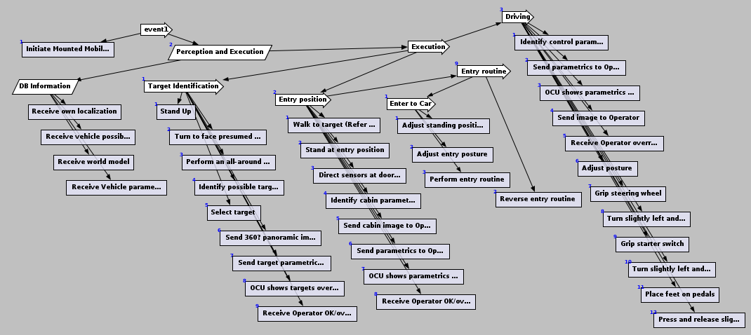
Figure 2: A plan for Drive challenge task, 47 nodes

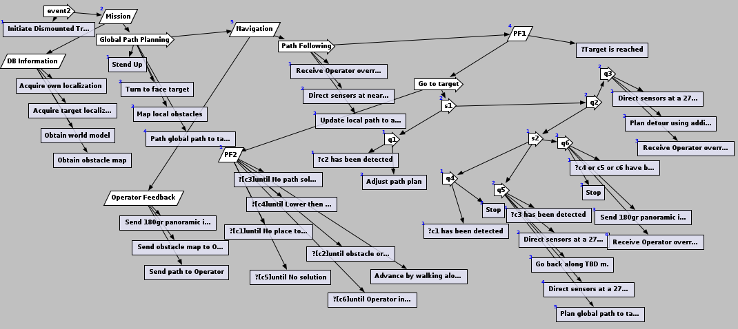
Figure 3: A plan for Walk challenge task, 57 nodes

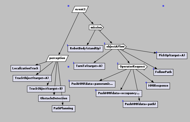
Figure 4: A plan for Pick-Up challenge task

In the Logistics domain, packages are to be transported by trucks or airplanes. Hierarchical plans were generated by the JSHOP2 planner [5] for this domain and consisted of one parallel node (packages delivered in parallel), with children all being sequential plans. In Figure 5 presented a simple plan generated by JSHOP2 algorithm for accomplishing (transport-two p1 p2) from the following initial state: $\{$(package p1), (at p1 l1), (destination p1 l3), (available-truck t1), (at t1 home), (package p2), (at p2 l2), (destination p2 l3), (available-truck t2), (at t2 home)$\}$. The duration distribution of all primitive tasks is uniform but the support parameters were determined by the type of the task, in some tasks the distribution is fixed (such as for load and unload) and in others the distribution depends on the velocity of the vehicle and on the distance to be travelled.

After running our approximation algorithm we also ran $\operatorname{Trim}_{L}$ which uses a reversed version of the $\operatorname{Trim}$ operator, providing a lower bound of the CDF, as well as the upper bound generated by Algorithm 6. Running both variants allows us to bound the actual error, costing only a doubling of the run-time. Despite the fact that our error bound is theoretically tight, in practice and with actual distributions, according to Tables 1 and  3, the resulting error in the algorithm was usually much better than the theoretical $\varepsilon$ bound.

We ran the exact algorithm, our approximation algorithm with $\varepsilon\in\{0.1,0.01,0.001\}$, and a simple simulation with $10^{3}$ to $10^{7}$ samples (number of samples is denoted by $s$ in the table), on networks from the DRC implementation, sequence nodes with 10, 20, and 50 children (number of nodes denoted by $N$ in the table), and 20 Logistics domain plans, and several values of $M$ (the notations $M,N$ are as in Theorem 4). Results for the various task trees are shown in tables 1, 3 (error comparison) and 2, 4 (runtime comparison). Errors are the maximum error in the CDF, measured from the true result when available, and from the bounds generated by the approximation algorithm using $\varepsilon=0.0001$ when the exact algorithm timed out (over 2 hours). The exact algorithm times out in many cases when the number of tasks is 20 or more, except when size of the support $M$ is very small, in which case it handles some more nodes, but still cannot handle 50 tasks even for $M=2$. Both our approximation algorithm and the sampling algorithm handle all these cases, as our algorithm’s runtime is polynomial in $N$, $M$, and ${1}/{\varepsilon}$ as is the sampling algorithm’s (time linear in number of samples).

The advantage of the approximation algorithm is mainly in providing bounds with certainty as opposed to the bounds in-probability provided by sampling. Additionally, as predicted by theory, accuracy of the approximation algorithm improves linearly with ${1}/{\varepsilon}$ (and almost linear in runtime), whereas accuracy of sampling improves only as a square root of the number of samples. Thus, even in cases where sampling initially outperformed the approximation algorithm, increasing the required accuracy for both algorithms, eventually the approximation algorithm overtook the sampling algorithm.

Figure 5: A simple plan generated by JSHOP2 algorithm.

Task Tree	$N$	$M$	Approximation algorithm error, given $\varepsilon$			Sample algorithm error, given # samples
			0.1	0.01	0.001	$10^{3}$	$10^{4}$	$10^{5}$	$10^{6}$	$10^{7}$
Drive	47	2	[-0.0052, 0.0086]	[-0.0004, 0.0004]	[-$3.2{\cdot}10^{-5}$, $3.4{\cdot}10^{-5}$]	0.0206	0.0072	0.0031	0.0009	0.0001
	47	4	[-0.0096, 0.019]	[-0.0009, 0.0013]	[-$9.2{\cdot}10^{-5}$, $1.3{\cdot}10^{-4}$]	0.0476	0.0075	0.0046	0.0011	0.0001
	47	10	[-0.014, 0.028]	[-0.0014, 0.0025]	[-$9.5{\cdot}10^{-5}$, $1.4{\cdot}10^{-4}$]	0.0236	0.0083	0.0024	0.0015	0.0003
Walk	57	2	[-0.0039, 0.004]	[-0.0003, 0.0003]	[-$3.1{\cdot}10^{-5}$, $3.2{\cdot}10^{-5}$]	0.0166	0.0067	0.002	0.0008	0.0003
	57	4	[-0.0038, 0.004]	[-0.0004, 0.0004]	[-$3.6{\cdot}10^{-5}$, $3.9{\cdot}10^{-5}$]	0.0232	0.0125	0.0022	0.0014	0.0003
	57	10	[-0.0047, 0.0049]	[-0.0004, 0.0005]	[-$3.8{\cdot}10^{-5}$, $4{\cdot}10^{-5}$]	0.0255	0.0117	0.0029	0.0011	0.0003
Pick Up	18	10	[-0.0041, 0.0061]	[-0.0003, 0.0005]	[-$3.5{\cdot}10^{-5}$, $5.8{\cdot}10^{-5}$]	0.018	0.0054	0.0027	0.0006	0.0002
	18	20	[-0.0038, 0.0031]	[-0.0006, 0.0005]	[-$3{\cdot}10^{-5}$, $3.5{\cdot}10^{-5}$]	0.027	0.0046	0.0015	0.0008	0.0002
Logistics1	34	2	[-0.0019, 0.0019]	0	0	0.0168	0.007	0.001	0.0009	0.0002
	34	4	[-0.0068, 0.0068]	[-0.0006, 0.0006]	[-$3.4{\cdot}10^{-5}$, $3.8{\cdot}10^{-5}$]	0.025	0.0057	0.0032	0.0005	0.0003
	34	10	[-0.008, 0.007]	[-0.0009, 0.0007]	0	0.018	0.011	0.003	0.0009	0.0004
Logistics2	45	2	[-0.002, 0.002]	0	0	0.013	0.015	0.004	0.001	0.0003
	45	4	[-0.004, 0.004]	[-0.0004, 0.0004]	[-$3.3{\cdot}10^{-5}$, $3.4{\cdot}10^{-5}$]	0.036	0.008	0.002	0.0006	0.0002
	45	10	[-0.005, 0.006]	[-0.0004, 0.0006]	0	0.03	0.013	0.002	0.001	0.0002

Table 1: Estimation errors

Task Tree	$N$	$M$	Exact	Approx. algorithm, with $\varepsilon$			Sampling algorithm, with # samples
				0.1	0.01	0.001	$10^{3}$	$10^{4}$	$10^{5}$	$10^{6}$	$10^{7}$
Drive	47	2	1.49	0.141	1.14	1.49	0.187	1.92	19.11	190.4	1905
	47	4	18.9	0.34	7.91	16.11	0.21	2.1	20.95	211.5	2113.6
	47	10	$>2$h	1.036	32.94	390.5	0.28	2.81	28.6	279.1	2844.4
Walk	57	2	4.46	0.33	3.1	4.03	0.205	2.06	20.86	208.1	2082.7
	57	4	183.5	0.983	18.42	95.11	0.23	2.34	23.03	230.4	2352.4
	57	10	$>2$h	8.13	128.99	3668.2	0.293	2.92	29.16	291.3	2902.7
Pick Up	18	10	5.76	0.022	0.193	1.133	0.103	0.983	9.8	101.9	1006.8
	18	20	27.88	0.046	0.4	3.15	0.132	1.33	13.25	130.4	1305.9
Logistics1	34	2	0.014	0.007	0.009	0.009	0.239	2.03	19.3	193.9	1767
	34	4	22.98	0.048	1.3	13.1	0.2	2	20	205	1928
	34	10	$>4$h	0.25	8.26	475	0.26	2.64	26.4	267	2649
Logistics2	45	2	0.07	0.02	0.06	0.06	0.23	2.35	23.4	234.7	2196
	45	4	373.3	0.2	7	82.9	0.25	2.5	25.6	256	2393
	45	10	$>4$h	2.19	120	6101	0.31	3.12	31.3	314	3139

Table 2: Runtime comparison (run times in seconds)

Task Tree	$N$	$M$	Approximation algo. error, given $\varepsilon$			Sample algo. error, given # samples
			0.1	0.01	0.001	$10^{3}$	$10^{4}$	$10^{5}$
Seq 10	10	4	[-0.027, 0.041]	[-0.0027, 0.0041]	[-$2.2{\cdot}10^{-4}$, $2.5{\cdot}10^{-4}$]	0.0224	0.008	0.0017
	10	10	[-0.0316, 0.0615]	[0.0033, 0.0067]	[$-2.6{\cdot}10^{-4}$, $5.2{\cdot}10^{-4}$]	0.027	0.0117	0.0038
Seq 20	20	2	[-0.02, 0.0373 ]	[-0.0015, 0.0026]	[-$1.6{\cdot}10^{-4}$, $2.6{\cdot}10^{-4}$]	0.0266	0.0077	0.003
	20	4	[-0.026, 0.025]	[-0.0025, 0.0025]	[-$2.7{\cdot}10^{-4}$, $2.3{\cdot}10^{-4}$]	0.039	0.01	0.002
	20	10	[-0.027, 0.027]	[-0.0028, 0.0027]	[-$3{\cdot}10^{-4}$, $2.5{\cdot}10^{-4}$]	0.032	0.007	0.0042
Seq 50	50	2	[-0.032, 0.032]	[-0.0028, 0.0028]	[-$2.8{\cdot}10^{-4}$, $2.4{\cdot}10^{-4}$]	0.0193	0.007	0.0024
	50	4	[-0.035, 0.035]	[-0.0036, 0.0035]	[-$3.9{\cdot}10^{-4}$, $3.2{\cdot}10^{-4}$]	0.0236	0.0064	0.0023
	50	10	[-0.037, 0.037]	[-0.004, 0.0039]	[-$4.2{\cdot}10^{-4}$, $3.5{\cdot}10^{-4}$]	0.017	0.007	0.005
Rand50-AVG	50	4	0.007	0.0007	0	0.0243	0.0084	0.0024

Table 3: Estimation errors for sequential plans

Task Tree	$N$	$M$	Exact	Approx. algorithm, with $\varepsilon$			Sample algorithm, with # samples
				0.1	0.01	0.001	$10^{3}$	$10^{4}$	$10^{5}$
Seq 10	10	4	0.23	0.003	0.02	0.148	0.054	0.545	5.336
	10	10	10.22	0.008	0.073	0.692	0.071	0.724	7.18
Seq 20	20	2	0.23	0.003	0.02	0.285	0.054	0.545	9.62
	20	4	$>2$h	0.011	0.106	1.208	0.105	1.066	10.74
	20	10	$>2$h	0.035	0.331	4.67	0.145	1.473	14.38
Seq 50	50	2	$>2$h	0.028	0.28	3.593	0.236	2.366	24.71
	50	4	$>2$h	0.079	0.81	11.145	0.265	2.68	26.84
	50	10	$>2$h	0.227	3.1	38.01	0.354	3.63	35.63
Rand50-AVG	50	4	$>2$h	1.1544	19.77	390.58	5.676	55.021	590.17

Table 4: Runtime comparison (run times in seconds) for sequential plans

9 Dependencies and other generalizations

Computing the distribution of the makespan in trees is considered a trivial problem in some contexts in probabilistic reasoning [16]. Specifically, given the task network, such as the one in Figure 6, it is straightforward to represent the distribution using a Bayes network (BN) that has one node per task where the children of a node $v$ in the task network are represented by BN nodes that are parents of the BN node representing $v$. This results in a tree-shaped BN, where it is well known that probabilistic reasoning can be done in time linear in the number of nodes, e.g., by belief propagation (message passing) [16, 17]. However, there is a difficulty, usually ignored in the UAI literature, in the potentially exponential size variable domains, which our algorithm, essentially a limited form of approximate belief propagation from primitive task variables to the root, avoids by trimming.

Figure 6: A simple task network.

Looking at makespan distribution computation as probabilistic reasoning leads immediately to the question on how to handle task completion times that have dependencies, represented as a BN. Since reasoning in BNs is NP-hard even for binary-valued variables [18, 19], this is hard in general. But for cases where the BN toplogy is tractable, such as for BNs with a small cutset,BNs with bounded treewidth [20], or directed-path singly connected BNs [21], a deterministic polynomial-time approximation scheme for the makespan distribution may be achievable.

Figure 7: A petri-net graph.

Figure 8: A non-hierarchical task network

Figure 9: Representing “shared” tasks using correlated random variables

Here we motivate and handle a special case of small cutsets. Specifically, suppose that, in addition to the tree, we allow a small number of dependencies between primitive task distributions. Does our algorithm generalize to this case? The importance of this question is because such an extension is natural in some contexts. For example, in the logistics case we have a 2-level tree, with a toplogy similar to that of Figure  6. The children of the sequence nodes are primitive tasks such as “drive delivery truck 1 from Boston to NY” (suppose this is primitive task A in Figure  6). Now, the duration of this action is a random variable that depends on the state of traffic at the time the action is taken. Suppose that another primitive action (e.g. primitive task C) is “drive delivery truck 2 from Boston to NY” which is to occur roughly at the same time as the first action. Since traffic conditions are likely to be very similar, the duration of the actions may be correlated, and we need to be able to take this dependency into account.

Another case where we have dependency is when the same primitive action is used in more than one composite task. Although this state cannot be represented in strict hierarchies, recall that timing relationships represented by HTNs can also be represented by directed acyclic perti nets. For example, the task network of Figure 6 can be represented by the perti net of Figure 7 (without the shaded arc). However, perti nets allow more general timing constraints: the language of trees is equlivalent to perti nets with a series-parallel graph structure. Adding the shaded arc from A to D in the petri net of Figure 7, we get a graph that is not series-parallel. Its equivalent in HTNs would be the non-tree structure shown in Figure 8, that shares primitive task A between composite tasks. The latter could be converted into a pure tree-shape by adding a task A’ that mirrors task A, i.e. has a duration exactly equal to that of A (Figure 9).

This case, as well as generalizations thereof where the number of correlated variables is small, we can handle by a scheme known as conditioning, adapted to our approximation scheme. For example, in cutset conditioning, a separate reasoning problem is generated for every possible value instantiation over all the cutset variables. The results are combined by weighted averaging. We propose to do the same in our case, but must prove that the approximation quality is maintained, as we indeed do below.

We thus assume that all primitive task durations are independent, when conditioned on a small cutset $Y$ of the primitive task durations. The joint duration distribution over $Y$ can be provided by a BN, or a complete table, or any other representation. We assume that the cardinality of the set $Y$ is sufficiently small that the joint domain size $m^{|Y|}$ is managable, in terms of memory and computation time if we have to iterate over all domain values. We are also given the duration distribution for any other task, given every possible value assignment $y$ to the variables in $Y$. Together, this information fully defines the joint probability of all the primitive task durations.

For example, in the case of Figure 9, we can set $Y=\{A\}$, so $Y$ is a singleton set. This is a somewhat degenerate example case, as the joint distribution can be represented trivially using $P(A^{\prime}=a^{\prime}|A=a)=1$, as all other primitive task duration variables are independent of $A$.

Let $X$ be the random variable denoting the makespan distribution of the root of the task network. We wish to estimate $F_{X}$, the cumulative distribution of $X$. Our approximation algorithms for trees without dependency can estimate an upper and lower bounds approximations. With dependencies, we cannot do so directly. However, consider an assignment $Y=y$, for some value $y\in D(Y)$. We are given the conditional distribution $Z|Y=y$ for all the rest of the primitive tasks, which are now independent given $Y=y$. Consider the distribution:

$$F_{X|Y=y}(x)=P(X\leq x|Y=y)$$

For each value $Y=y$ we can run the approximation algorithm, to get upper Kolmogorov bound $F_{X^{+}|Y=y}(x)$ and lower Kolmogorov bound $F_{X^{-}|Y=y}(x)$. Due to Theorem 3, we have the following property, for all $x$:

$$F_{X^{+}|Y=y}(x)\succeq_{\varepsilon}F_{X|Y=y}(x)\succeq_{\varepsilon}F_{X^{-}|Y=y}(x)$$

Now let:

$$F_{X^{-}}(x)=\sum_{y\in D(Y)}P_{Y}(y)F_{X^{-}|Y=y}(x)$$

and likewise:

$$F_{X^{+}}(x)=\sum_{y\in D(Y)}P_{Y}(y)F_{X^{+}|Y=y}(x)$$

Theorem 10.

Computing $F_{X^{-}}(x)$ and $F_{X^{+}}(x)$ takes time $O(m^{|Y|})t$, where $t$ is the runtime of our tree task network algorithm. The resulting approximation obeys, for all $x$:

$$F_{X^{+}}(x)\succeq_{\varepsilon}F_{X}(x)\succeq_{\varepsilon}F_{X^{-}}(x)$$

Proof.

The runtime bound is obvious, as a trivial implementation simply takes $m^{|Y|}$ runs of the tree task network algorithm. The approximation bounds follow from the bounds for individual values $Y=y$, and from a convexity argument. For example, by construction, we have:

$$F_{X^{-}}(x)-F_{X}(x)=\sum_{y\in D(Y)}P_{Y}(y)(F_{X^{-}|Y=y}(x)-F_{X|Y=y}(x))$$

The right hand side is a convex sum of quantities that are all between 0 and $\varepsilon$, which therefore must also be between 0 and $\varepsilon$. ∎

10 Discussion

We proposed an operator for trimming the support of random variables such that the resulting trimmed variable is an approximation of the variable that has a bigger support. As the motivation in this paper was to estimate the probabilities of meeting deadlines in hierarchical plans, the notion of approximation used is a one-sided version of the Kolmogorov metric, that reflects the fact that in such estimations we allow over-, not under- approximations. The core of the paper is devoted to an analysis of the prorogation of the estimation errors in the computation of the random variable that represents the makespan of a hierarchical plan. Based on this analysis, the paper proposes recursive algorithms that can compute an approximation of this makespan in time and memory that are polynomial in the sizes of the supports of the primitive tasks, the size of the tree, and of the inverse of the required accuracy ($1/\varepsilon$).

In the following paragraphs we discuss directions for future research and ideas for possible technical improvements of the proposed techniques. Some of these improvements are easy to implement and the reason for not including them in the first place was for clarity of the presentation, other require future research.

Avoid trimming variables with a small support

In the proposed algorithm, for ease of analysis and because we wanted to keep the code simple, we trimmed all the input and intermediate variables, whatever the size of their support is. This may be required, in a worst case, so doing so does not affect the complexity results, but it may give inferior run time and memory performance in the average case. We therefore, recommend to only trim variables that are small. This can be added as an initial test inside the Trim procedure.

Add a trim after a parallel node

Another point is that in the combined algorithm, space and time complexity can be reduced by adding some $\operatorname{Trim}$ operations, especially after processing a parallel node, which is not done in our version. This may reduce accuracy, a trade-off yet to be examined.

Focused trimming

Another option is, when given a specific threshold, trying for higher accuracy in just the region of the threshold, but how to do that is non-trivial. For sampling schemes such methods are known, including adaptive sampling [22, 23], stratified sampling, and other schemes. It may be possible to apply such schemes to deterministic algorithms as well - an interesting issue for future work.

Extension to continuous distributions

Our algorithm can handle them by pre-running a version of the $\operatorname{Trim}$ operator on the primitive task distribution. Since one cannot iterate over support values in a continuous distribution, start with the smallest support value (even if it is $-\infty$), and find the value at which the CDF increases by $\varepsilon$. This requires access to the inverse of the CDF, which is available, either exactly or approximately, for many types of distributions.

Approximating expectations

We showed that the expectation problem is also NP-hard. A natural question is on approximation algorithms for the expectation problem, but the answer here is not so obvious. Sampling algorithms may run into trouble if the target distribution contains major outliers, i.e. values very far from other values but with extremely low probability. Our approximation algorithm can also be used as-is to estimate the CDF and then to approximate the expectation, but we do not expect it to perform well because our current $\operatorname{Trim}$ operator only limits the amount of probability mass moved at each location to $\varepsilon$, but does not limit the “distance” alnog the $x$ parameter over which it is moved. The latter may be arbitrarily bad for estimating the expectation. Nevertheless, a different version of $\operatorname{Trim}$ that bounds just this distance was shown to provide a polynomial-time approximation scheme for the expectations in EXPECTI-MIN-MAX game trees [24], if the utilities are bounded. Since the expectation operator involves convolution, these results should be applicable (with some adjustment) to task networks as well.

Optimal trimming

While we proved that the trimming procedure proposed in this paper allows for approximation that improves polynomially with the time and memory invested. It is interesting to look for optimal approximations. In [25], we showed that an optimal approximation of a single random variable can be obtained in polynomial time. Specifically, we showed that given a random variable $X$ and a target support size $m$, we can find the minimal $\varepsilon^{*}$ and a variable $X^{\prime}$ such that $X^{\prime}$ has support of size $m$ and $X\prec_{\varepsilon^{*}}X^{\prime}$. Note that this does not directly give an optimal approximation of the makespan of a complete plan.

Compact representations of the random variables

One can view the work presented in this paper in the context of function approximation. In general, a function approximation problem is about the selection a function among a well-defined class that approximates a target function in a certain way. In our case, we approximate the CDF of a random variable with a piecewise constant function with a small number of pieces. As in other applications of function approximation, it is natural to ask whether more compact representations of the random variable exist. For example one can represent functions in a compressed from where a repeated entry can be specified once with a number that specifies the number of repetitions. Another approach would be to approximate using, e.g., splines instead of constant lines. The challenge will be, in any of these variants, to work directly on the compressed representation, as we do in this paper.

Split weights

In the proposed $\operatorname{Trim}$ algorithm, the inner loop goes until $p+prob(d)\leq\varepsilon$ and, when this condition is not met, the value of $prod(d)$ is left for the next iteration. A possible improvement, not included in the base version for simplicity, is to add to $p$ the part of $prob(d)$ up to $\varepsilon$ (i.e., have $p=\varepsilon$) and leave only the remaining part of $prob(d)$ to the next iteration.

11 Related work

We outline previous work on HTN planning, series-parallel networks, scheduling with uncertain task durations, the sum and the maximum of random variables, and approximation schemes.

HTN (Hierarchical Task Network)

Some task network models include, beyond the nodes that we handled in this paper, constraints on the tasks that restrict how some of the variables can be bound and the order in which parallel tasks are to be performed [3, 26, 11]. In [3] Erol et al., formally define, analyze and explicate features of the design of HTN planning systems. Specifically, how is the complexity of HTN planning varies with various conditions on the task networks. Our construction, at moment, supports only the basic structure. Methods for solving HTN are suggested as an online planning [4, 5, 2] and as offline planning [6]. In the experiments we conducted, we used hierarchical plans obtained by SHOP2 [5] planner in the “Logistics” domain from IPC2 (http://ipc.icaps-conference.org/). The SHOP2 (Simple Hierarchical Ordered Planner 2) is a domain-independent planning system based on Hierarchical Task Network (HTN) planning. There are other HTN planners like TLPLan or TALPlanner  [27] but we chose, for convenience, to use JSHOP2, the Java version of SHOP2.

Series-parallel networks

There has been much work on series-parallel networks, although not all related to planning or AI. In [28], Gelenbe discusses the fundamental issues involved in the performance of parallel computers. We believe that our work can be applied also in this context. Specifically, in Chapter 5 of this book Gelenbe proposes a model for series-parallel processing structures. Programs in this model are composed of (primitive) tasks; some of them are to be performed in series, others may be performed in parallel. Given the execution time distribution of each task (assuming i.i.d) and the characteristic parameters of the branching process, a method for computing numerically the execution time distribution of the program is shown. The computation involves numerical solutions based on solving a differential-integral equation and iterative methods. In [29], which is based on the same model, a bound on the average total execution time of a series–parallel processing structure is presented. Both papers are very relevant to our work and contributed as case studies (not reported directly in this paper). Moreover, this type of work supplies another motivation for the work shown in this paper. Temporal planing and in particular TPNs (temporal plan network) are presented in [30], the model is similar to ours, but the focus is on lower/upper bounds, rather than probability distributions. Hierarchical constraint-based plans in MAPGEN [31] allow for more general dependencies than series-parallel, providing additional expressive power but making the deadline problem even harder.

Scheduling under uncertainty

Scheduling and in particular, scheduling under uncertainty, can provide additional motivation to our work. In [32] Herroelen and Leus review approaches for scheduling under uncertainty such as reactive scheduling and stochastic project scheduling and discuss the potentials of these approaches for scheduling under uncertainty of projects (tasks) with deterministic network evolution structure. Another relevant paper is [33] which provides computational complexity results for two PERT problems. Here a project is specified by precedence relations among tasks and task durations specified as discrete independent random variables. Three results are obtained: computing a value of the cumulative distribution function of project duration is #P-complete, computing the mean of the distribution is at least as hard, and neither of the problems can be computed in time polynomial in the number of points in the range of the project duration. This paper deals with a more general problem than ours, and with a different type of complexity. Our results are orthogonal, because we show a source of complexity that is not in the graph structure but in the distributions themselves. In fact, the 2-state problem shown to be hard for general graphs by Hagstrom, can be solved in polynomial time for series-parallel trees by dynamic programming. Another relevant paper is [34] which allows to represent each activity by an independent random variable with a known mean and variance. The best solutions are ones which have a high probability of achieving a good makespan, and methods for combining Monte Carlo simulation with deterministic scheduling algorithms are shown. Compared to our results, the bounds given in [34] are all in terms of the probability of errors while we bound the errors absolutely. In [35] RCPSP/max (Resource Constrained Project Scheduling Problems with minimum and maximum time lags) is studied, where the durations of activities are not known with certainty. Similarly, in [7] a simulation approach is used to evaluate the expected makespan of a number of Partial Order Schedules (POS). The evaluation in the paper shows correlation between the expected makespan and the makespan obtained by simply fixing all durations to their average. The authors of this paper claim that the correlation that they report on allows to use averages instead of the random variables and yet obtain a very accurate estimation of the expected makespan. This, of course, is due to the linearity of expectation, that does not carry when working with other operators such as maximum. Another disadvantage of using averages or sampling is that they cannot give formal guarantees needed, e.g, in Service-Level-Agreements (SLA) where guarantees of the form: “response time is less than 1mSec in at least 95% of the cases” are common [8]. A few aspects distinguish our work from the presented scheduling papers. First, both [35] and [7] provide guarantees only in probability. These are good for application where such guarantees are sufficient while we provide stronger guarantees. Second, our work is on approximating CDF, i.e., the probability of missing deadlines. Clearly, unlike expectations, this cannot always be directly derived from averages and variances as in [7] or by sampling as in [34]. For example, consider the following two tasks. Task A whose duration is 10 seconds with probability 0.999 or 20 seconds with probability 0.001. And task B whose duration is 10.02 seconds with probability 0.999 or 0.02 seconds with probability 0.001. Clearly, these two random variables have the same expectation (10.01) and even the same variance (0.01998). Of course, the averages of samples of these variables should be close to their expectations. But, if we take, say, ten tasks of A in sequence, we get a probability close to zero of crossing a deadline of 100.1 and if we take ten tasks of B in sequence, we get that the probability to cross this deadline is almost 1.

Sum and Max of random variables

Various works exist in the research literature regarding the sum and the maximum of random variables. For example, Evans and Leemis [36] present algorithms for computing the exact probability density function of the sum of two independent discrete random variables and show an implementation of the algorithm in a computer algebra system. This paper does not examine the case of summing more than two discrete random variables which is our main challenge. However, there are other papers that handle the case of summing more than two random variables like [37] which examines the sum of Bernoulli distributed random variables. They present a simple derivation for an exact formula with a closed-form expression for the CDF of the Poisson binomial distribution. The derivation uses the discrete Fourier transform of the characteristic function of the distribution. Numerical studies were conducted to study the accuracy of the developed algorithm and approximation methods. For example Bromiley [38] examines the sum of normally distributed random variables. The fact that the product and the convolution of Gaussian probability density functions (PDFs) are also Gaussian functions, is well known. Bromiley provides proofs that the following cases are also Gaussian functions: the product of two univariate Gaussian PDFs, the product of an arbitrary number of univariate Gaussian PDFs, the product of an arbitrary number of multivariate Gaussian PDFs, and the convolution of two univariate Gaussian PDFs. Note that this list does not include the maximum of two variables. In fact, we are not aware of any representation of random variables, except for the implicit PMF table used in this paper, that is closed under addition and under maximum. Mercier [39] proposes algorithms for computing bounds of cumulative density functions of sums of i.i.d. non-negative random variables, renewal functions and cumulative density functions of geometric sums of i.i.d. non-negative random variables. Our work allows for non identical variables. Distribution of the maximum of random variables are discussed in [40], with a focus mostly on continuous distributions. All the above papers treat either the sum of random variables or the maximum of random variables but not both together.

Approximation algorithms

Our work also relates to FPTAS (fully polynomial-time approximation schemes) [15] approximation algorithms for the, so called, knapsack problem [41, 42, 43]. The idea of FPTAS for knapsack is to scale the profits downwards enough so the profits of all the objects are polynomially bounded in $n$ and then to use dynamic programming on the new instance. By scaling with respect to a desired $\varepsilon$, the solution is at least $(1-\varepsilon)\cdot OPT$ where $OPT$ is the optimal solution, in polynomial time with respect to both $n$ and $1/\varepsilon$. Our binning technique is similar. Another algorithm that uses a similar binning technique, for a variant of the, so called, subsetsum problem, is described in [44]. This subsetsum variant is a decision problem, given a set of $n$ numbers $x_{1},\cdots x_{n}$, a target $t$ and $0\leq\varepsilon\leq 1$, return yes, if there is a subset that sums between $(1-\varepsilon)t$ and $t$. In this context, FPTAS “trimming” is to remove values that are close to each other. In other words, if two values $s_{1}$ and $s_{2}$ that represent a sum of subset of $S$ are close to each other, then for the purpose of finding an approximate solution there is no reason to maintain both of them, so it is possible to merge them to be represented by $s_{1}$ or $s_{2}$ and delete the other. The idea in our approximation algorithm is similar to this. In [15], Chapter 9 “complexity of counting”, the complexity class #P is presented and examples for counting problems are given, e.g., #knapsack problem (defined in Chapter 7). Another type of approximation is FPRAS, studied e.g., in [45] which presents an algorithm that uses dynamic programming to provide a deterministic relative approximation and then sampling techniques to give arbitrary approximation ratios and  [46] that uses Markov chain Monte Carlo technique. The research literature also contains numerous randomized approximation schemes that handle dependencies [16, 47], especially for the case with no evidence. In fact, our implementation of the sampling scheme in ROBIL handled dependent durations. It is unclear whether such sampling schemes can be adapted to handle dependencies and arbitrary evidence, such as: “the completion time of compound task $X$ in the network is known to be exactly one hour from now”. Another type of approximation algorithms uses Monte-Carlo technique as presented, e.g., in [22, 23].

Acknowledgments.

This research was supported by the ROBIL project, and by the Lynne and William Frankel Center for Computer Science at Ben-Gurion University.

Refferences

References

- [1] L. Cohen, S. E. Shimony, G. Weiss, Estimating the probability of meeting a deadline in hierarchical plans, in: Twenty-Fourth International Joint Conference on Artificial Intelligence, 2015.
- [2] A. Gabaldon, Programming hierarchical task networks in the situation calculus, in: AIPS’02 Workshop on On-line Planning and Scheduling, 2002.
- [3] K. Erol, J. Hendler, D. S. Nau, HTN planning: Complexity and expressivity, in: AAAI, 1994.
- [4] D. S. Nau, S. J. Smith, K. Erol, et al., Control strategies in HTN planning: Theory versus practice, in: AAAI/IAAI, 1998, pp. 1127–1133.
- [5] D. S. Nau, T.-C. Au, O. Ilghami, U. Kuter, J. W. Murdock, D. Wu, F. Yaman, SHOP2: An HTN planning system, J. Artif. Intell. Res. (JAIR) 20 (2003) 379–404.
- [6] J. P. Kelly, A. Botea, S. Koenig, Offline planning with Hierarchical Task Networks in video games., in: AIIDE, 2008, pp. 60–65.
- [7] A. Bonfietti, M. Lombardi, M. Milano, Disregarding duration uncertainty in partial order schedules? Yes, we can!, in: CPAIOR, 2014, pp. 210–225.
- [8] R. Buyya, S. K. Garg, R. N. Calheiros, SLA-oriented resource provisioning for cloud computing: Challenges, architecture, and solutions, in: Cloud and Service Computing (CSC), 2011.
- [9] R. Möhring, Scheduling under uncertainty: Bounding the makespan distribution, Computational Discrete Mathematics (2001) 79–97.
- [10] H. W. Lilliefors, On the Kolmogorov-Smirnov test for normality with mean and variance unknown, Journal of the American Statistical Association 62 (318) (1967) 399–402.
- [11] S. J. Russell, P. Norvig, Artificial Intelligence: A Modern Approach, 2nd Edition, Pearson Education, 2003.
- [12] R. Simmons, Planning, Execution & Learning 1. Linear & Non-Linear Planning, (Script). Carnegie Mellon University, USA.
- [13] E. Aktolga, A java planner for blocksworld problems, University of Osnabrueck.
- [14] M. R. Garey, D. S. Johnson, Computers and Intractability; A Guide to the Theory of NP-Completeness, W. H. Freeman & Co., NY, USA, 1990.
- [15] S. Arora, B. Barak, Computational complexity: a modern approach, Cambridge University Press, 2009.
- [16] J. Pearl, Probabilistic Reasoning in Intelligent Systems: Networks of Plausible Inference, Morgan Kaufmann, San Mateo, CA, 1988.
- [17] J. H. Kim, J. Pearl, A computation model for causal and diagnostic reasoning in inference systems, in: IJCAI, 1983.
- [18] P. Dagum, M. Luby, Approximating probabilistic inference in Bayesian belief networks is NP-hard, Artificial Intelligence 60 (1) (1993) 141–153.
- [19] G. F. Cooper, The computational complexity of probabilistic inference using Bayesian belief networks, Artificial Intelligence 42 (2-3) (1990) 393–405.
- [20] H. L. Bodlaender, Treewidth: Characterizations, applications, and computations, in: WG, 2006, pp. 1–14.
- [21] S. E. Shimony, C. Domshlak, Complexity of probabilistic reasoning in directed-path singly connected Bayes networks, Artificial Intelligence 151 (2003) 213–225.
- [22] C. G. Bucher, Adaptive sampling: an iterative fast Monte Carlo procedure, Structural Safety 5 (2) (1988) 119–126.
- [23] R. J. Lipton, J. F. Naughton, D. A. Schneider, Practical selectivity estimation through adaptive sampling, Vol. 19, ACM, 1990.
- [24] S. S. Shperberg, S. E. Shimony, A. Felner, Monte-carlo tree search using batch value of perfect information.
- [25] L. Cohen, T. Grinshpoun, G. Weiss, Optimal approximation of random variables for estimating the probability of meeting a plan deadline, in: AAAI, 2018.
- [26] K. Erol, J. Hendler, D. S. Nau, Complexity results for HTN planning, Annals of Mathematics and Artificial Intelligence 18 (1) (1996) 69–93.
- [27] J. Kvarnström, P. Doherty, TALplanner: A temporal logic based forward chaining planner, Annals of Mathematics and Artificial Intelligence 30 (1-4) (2000) 119–169.
- [28] E. Gelenbe, Multiprocessor performance, Wiley, 1989.
- [29] W. J. Gutjahr, G. C. Pflug, Average execution times of series–parallel networks, Séminaire Lotharingien de Combinatoire 29 (1992) 9.
- [30] P. Kim, B. C. Williams, M. Abramson, Executing reactive, model-based programs through graph-based temporal planning, in: IJCAI, 2001, pp. 487–493.
- [31] M. Ai-Chang, J. Bresina, L. Charest, A. Chase, J. Cheng-jung Hsu, A. Jonsson, B. Kanefsky, P. Morris, K. Rajan, J. Yglesias, B. G. Chafin, W. C. Dias, P. Maldague, Mapgen: Mixed-initiative planning and scheduling for the mars exploration rover mission 19 (2004) 8–12.
- [32] W. Herroelen, R. Leus, Project scheduling under uncertainty: Survey and research potentials, European journal of operational research 165 (2) (2005) 289–306.
- [33] J. N. Hagstrom, Computational complexity of PERT problems, Networks 18 (2) (1988) 139–147.
- [34] J. C. Beck, N. Wilson, Proactive algorithms for job shop scheduling with probabilistic durations., J. Artif. Intell. Res.(JAIR) 28 (2007) 183–232.
- [35] N. Fu, P. Varakantham, H. C. Lau, Towards finding robust execution strategies for RCPSP/max with durational uncertainty., in: ICAPS, 2010, pp. 73–80.
- [36] D. L. Evans, L. M. Leemis, Algorithms for computing the distributions of sums of discrete random variables, Mathematical and Computer Modelling 40 (13) (2004) 1429–1452.
- [37] Y. Hong, On computing the distribution function for the poisson binomial distribution, Computational Statistics & Data Analysis 59 (2013) 41–51.
- [38] P. A. Bromiley, Products and convolutions of gaussian probability density functions (2013).
- [39] S. Mercier, Discrete random bounds for general random variables and applications to reliability, European j. of operational research 177 (1) (2007) 378–405.
- [40] L. Devroye, Generating the maximum of independent identically distributed random variables, Computers & Mathematics with Applications 6 (3) (1980) 305–315.
- [41] K. Lai, M. Goemans, The knapsack problem and fully polynomial time approximation schemes (FPTAS), Retrieved November 3 (2006) 2012.
- [42] E. L. Lawler, Fast approximation algorithms for knapsack problems, Mathematics of Operations Research 4 (4) (1979) 339–356.
- [43] P. Gopalan, A. Klivans, R. Meka, D. Stefankovic, S. Vempala, E. Vigoda, An FPTAS for# knapsack and related counting problems, in: Foundations of Computer Science (FOCS), 2011 IEEE 52nd Annual Symposium on, IEEE, 2011, pp. 817–826.
- [44] T. H. Cormen, C. Stein, R. L. Rivest, C. E. Leiserson, Introduction to Algorithms, 2nd Edition, McGraw-Hill Higher Education, 2001.
- [45] M. Dyer, Approximate counting by dynamic programming, in: Proceedings of the thirty-fifth annual ACM symposium on Theory of computing, ACM, 2003, pp. 693–699.
- [46] B. Morris, A. Sinclair, Random walks on truncated cubes and sampling 0-1 knapsack solutions, SIAM journal on computing 34 (1) (2004) 195–226.
-
[47]
C. Yuan, M. J. Druzdzel,
Importance
sampling algorithms for Bayesian networks: Principles and performance,
Mathematical and Computer Modelling 43 (9–10) (2006) 1189 – 1207.
doi:http://dx.doi.org/10.1016/j.mcm.2005.05.020.
URL http://www.sciencedirect.com/science/article/pii/S0895717705005443