Nonparametric inference in a stereological model with oriented cylinders applied to dual phase steel

Abstract

Oriented circular cylinders in an opaque medium are used to represent certain microstructural objects in steel. The opaque medium is sliced parallel to the cylinder axes of symmetry and the cut-plane contains the observable rectangular profiles of the cylinders. A one-to-one relation between the joint density of the squared radius and height of the 3D cylinders and the joint density of the squared half-width and height of the observable 2D rectangles is established. We propose a nonparametric estimation procedure to estimate the distributions and expectations of various quantities of interest, such as the cylinder radius, height, aspect ratio, surface area and volume from the observed 2D rectangle widths and heights. Also, the covariance between the radius and height of a cylinder is estimated. The asymptotic behavior of these estimators is established to yield point-wise confidence intervals for the expectations and point-wise confidence sets for the distributions of the quantities of interest. Many of these quantities can be linked to the mechanical properties of the material, and are, therefore, useful for industry. We illustrate the mathematical model and estimation procedures using a banded microstructure for which nearly 90 µm of depth have been observed via serial sectioning.

FLA

, and T1Supported under project number M41.10.09330 in the framework of the Research Program of the Materials innovation institute M2i (www.m2i.nl).

1 Introduction

One of the biggest challenges of studying materials like steel is the inability to see inside of an opaque medium. While there are methods to obtain three-dimensional (3D) information, they tend to be costly both in terms of time and resources. Methods like serial sectioning are destructive to the material and require long periods of time to collect a reasonable amount of data. Nondestructive methods such as synchotron radiation are expensive and can only be performed at specialized laboratories. The discipline of stereology provides many tools to confront these issues in the sense that there are well established models that provide means of estimating various 3D quantities based on (relatively inexpensive) two-dimensional (2D) observations and measurements; see, for example, Mayhew (1991), Ohser and Mücklich (2000), Russ and Dehoff (2000). A classical example comes from a study by Wicksell (1925) where the size distribution of spherical corpuscles in spleens is estimated based on measuring the circular cross-sections from slices of the spleens. Wicksell derived the relationship between the distribution of the unobservable sphere radii and the distribution of the observable cross-sectional circle radii. He then used the empirical data and a histogram estimator to solve his particular problem.

This basic stereological model has been applied in a variety of disciplines where it is not possible to obtain full 3D measurements of objects simply by looking at them; this includes biology, geology, astronomy and materials science: [Cruz-Orive and Weibel (1990), Giumelli, Militzer and Hawbolt (1999), Higgins (2000), Jeppsson et al. (2011), Miyamoto (1994), Sahagian and Proussevitch (1998), Sen and Woodroofe (2012), Tewari and Gokhale (2001)]. Not surprisingly, the method has also gained considerable attention in the statistics literature. There, the main focus is on computation and asymptotic behavior of the proposed estimators [Cruz-Orive et al. (1985), Mase (1995), Sen and Woodroofe (2012), Silverman et al. (1990), van Es and Hoogendoorn (1990)].

In several applications the particles of interest are spheres, or close enough to be treated as such. However, in many other applications the particles are not spherical at all, and so it is important to also consider models with nonspherical particles. The basic model with spheres has been extended to randomly oriented cylinders, polygons, spheroids and ellipsoids, and nonregular shapes [Andersen, Holme and Marioara (2008), Fullman (1953), Higgins (2000), Giumelli, Militzer and Hawbolt (1999), Li et al. (1999), Jensen (1995), Mehnert, Ohser and Klimanek (1998), Oakeshott and Edwards (1992), Sahagian and Proussevitch (1998), Spiess and Spodarev (2011), Thouless, Dalgleish and Evans (1988)].

All of this has led to a large body of work from which information of interest to scientists, engineers and industry can be drawn. The tools that have been created are powerful in their versatility. They can be applied to real materials, to models and simulations. They can also be studied from a theoretical point of view. The specific motivation for this current work comes from banded steel microstructures, like the one shown in Figure 1. The industry is interested in this particular material because it has anisotropic properties, high susceptibility to cracking and corrosion, and it is more difficult to machine than nonbanded material. This anisotropy can arise either from the particular chemistry of the steel or during the rolling phase when blocks of steel are flattened into sheets and rolled into coils. Currently, there is no reliable way to prevent or control the banding under certain necessary processing environments. Being able to quantitatively describe the sizes of the bands in 3D will greatly aid industry in assessing the quality of the material and the extent of the effects the bands have on the material coming off the production line. Ultimately, this will also aid in understanding and controlling the process that leads to band formation, thereby making it possible to eliminate them from the material when they are undesirable.

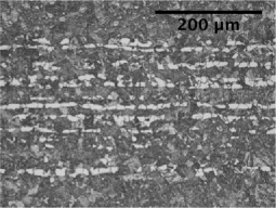
Figure 1: Optical image of a banded steel microstructure.

In this paper, we propose a simple model in which we use randomly sized, oriented cylinders to represent the microstructural bands. Following the example set forth by Wicksell (1925) when he considered spherical corpuscles observed in spleens, we will consider the marginal distributions of the radius and height of the cylinders. While most stereological models assume that nonspherical objects are randomly oriented, in this case, it is clear that this assumption is not appropriate. Therefore, by imposing the orientation constraints, we can explore other properties of the cylinders, such as the volume, surface area and aspect ratio. These quantities are important to estimate because they are linked to the mechanical properties of the material. For example, the surface area can be linked to the interface area between two phases, which determines properties like strength and resistance to corrosion or cracking.

In this work, we propose two nonparametric estimators for estimating the distributions of the 3D cylinder quantities of interest from the 2D rectangle observations. One estimator enforces a monotonicity constraint, inspired by the work of Groeneboom and Jongbloed (1995), the other does not. An empirical estimator is used to estimate the expectations of the 3D quantities of interest from the 2D observations. The rates of convergence and asymptotic distributions for all of these estimators are derived, which provide means of estimating the point-wise confidence intervals for the expectations and point-wise confidence sets for the distributions when the model is applied to the steel microstructures. While a parametric estimator could perform better than the nonparametric estimators we propose here, not enough is known about the bands within steel microstructures to assume any particular distribution for the radius and height of the cylinders. Therefore, the first step toward understanding this distribution is to study it nonparametrically and so this work focuses on the empirical and isotonic estimators for understanding the material.

This paper is organized as follows. The cylinder model is introduced in Section 2. The nonparametric estimation procedures is described in Section 3 and the asymptotic distributions and rates of convergence of the two different estimators are derived in Sections 4 and 5. A simulation for validation of the model is presented in Section 6 and, finally, in Section 7 the model is applied to the banded microstructure.

2 Cylinder model

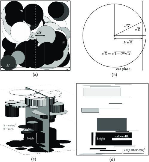
Figure 2: Visualization of the cylinder model. (a) Top view of cylinders in an $M\times M\times M$ box with a cut plane (dashed line) and slab $S_{x}$ (solid lines) into which cylinder centers should fall to be cut by the plane. (b) Schematic view, $\sqrt{X}$ is the cylinder radius, $\sqrt{Z}$ is the rectangle half-width, $U$ is a uniform random variable. (c) View of cut plane through the box. (d) Observations on the cut plane.

To represent the bands shown in Figure 1, the following model is proposed (see Figure 2). Cylinders are generated with a joint density $f$ for the squared radius $X$ [the choice to look at the squared radius is inspired by Hall and Smith (1988)] and height $H$. The centers of these cylinders are cylinders are placed such that their axes of symmetry all have the same orientation, as in Figure 2(c). A cylinder with radius $\sqrt{x}$ will be intersected by the plane if and only if its center falls within slab $S_{x}$ as shown in Figure 2(a). This leads to biased observations on the cut plane since cylinders with larger radii have a higher probability of being intersected. More specifically, the joint cumulative distribution function (CDF) of $(X,H)$, given that the plane intersects the cylinder, can be written as

$$P(X\leq x,H\leq h|\mbox{cylinder hits plane})$$

$$\qquad=\frac{P(X\leq x,H\leq h\mbox{ and cylinder hits plane})}{P(\mbox{cylinder hits plane})}$$

$$\qquad=\frac{\int_{y=0}^{x}\int_{m=0}^{h}\sqrt{y}f(y,m)\,dm\,dy}{\int_{y=0}^{\infty}\int_{m=0}^{\infty}\sqrt{y}f(y,m)\,dm\,dy}$$

$$\qquad=\frac{1}{m_{F}^{+}}\int_{y=0}^{x}\int_{m=0}^{h}\sqrt{y}f(y,m)\,dm\,dy.$$

Here, since the probability that the cylinder is cut is proportional to the radius, the density function $f$ is weighted by the ratio of the radius of the cylinder, $\sqrt{x}$, to the expected radius, $E_{f}[\sqrt{X}]\equiv m_{F}^{+}$, which we assume to be finite (see Assumption 1). Since the centers of the circles are uniformly distributed throughout the medium, the distance from the center of a cylinder that has been cut to the intersecting plane is a uniform random variable, as shown in Figure 2(b). This is analogous to the relationship between the circle radii and sphere radii in the method set forth by Wicksell (1925). Once a cylinder has been cut, the observable portion is seen as a rectangle on the cut plane, as shown in Figure 2(d).

The rectangles have observable squared half-widths, $z$, and heights, $h$, that have a joint density $g$. Since the cylinders are all cut parallel to their axis, all of the height information for the cut cylinders is preserved and directly observable on the cut-plane. (This shows that the distribution of the cylinder centers along the direction of the heights does not require the uniform random assumption.) The half-widths of the observed rectangles are related to the cylinder radii through the relationship displayed in Figure 2(b). From these 2D observations, one can estimate the 3D distribution where the relationship between $g$ and $f$ can be obtained using a variant of the well-known formula relating the density of the rectangle half-width (and height) to the distance of cylinder center to the cut plane and the density of the cylinder radius (and height):

$$g(z,h) = \frac{\int_{x=z}^{\infty}(x-z)^{-{1}/2}f(x,h)\,dx}{2\int_{x=0}^{\infty}\sqrt{x}f_{X}(x)\,dx}$$

$$= \frac{1}{2m_{F}^{+}}\int_{x=z}^{\infty}(x-z)^{-{1}/2}f(x,h)\,dx.$$

This relation can be inverted to obtain the joint density for the cylinder radius and height as a function of the observable rectangle joint density:

$$f(x,h) = -\frac{\partial}{\partial x}\frac{\int_{z=x}^{\infty}(z-x)^{-{1}/2}g(z,h)\,dz}{\int_{z=0}^{\infty}z^{-{1}/2}g_{Z}(z)\,dz}$$

$$= -\frac{1}{m_{G}^{-}}\frac{\partial}{\partial x}\int_{z=x}^{\infty}(z-x)^{-{1}/2}g(z,h)\,dz,$$

where $m_{G}^{-}\equiv E[Z^{-1/2}]$ is the expectation of one over the rectangle half-width and is also assumed to be finite (see Assumption 1). From this relationship, the distributions of univariate quantities of interest such as the height $H$, the squared radius $X$, the aspect ratio $R=\sqrt{X}/H$, the surface area $S=2\pi(X+\sqrt{X}H)$, and the volume $V=\pi XH$ can be calculated.

The CDF for the observed height takes on the form

$$F_{H}(h)=\int_{t=0}^{h}f_{H}(t)\,dt=\frac{1}{m_{G}^{-}}\int_{t=0}^{h}\int_{z=0}^{\infty}z^{-{1}/2}g(z,t)\,dz\,dt.$$ (3)

Note that this CDF still contains the weight associated with the bias from the radius of the cylinder. This accounts for any dependence that might exist between the cylinder height and radius. Should such a dependence exist, the observed rectangle height distribution will also be biased. See Figure 4 and Section 4.4 for a more detailed discussion of the biasing of the height observations associated with a dependence of the height and radius.

For each of the other quantities of interest, define

$$\qquad q(h;t)=\cases{t,&\quad(squared radius $T=X$),\vspace*{3pt}\cr(ht)^{2},&\quad(aspect ratio $T=\sqrt{X}/H$),\vspace*{5pt}\cr\displaystyle\biggl{[}\sqrt{\frac{h^{2}}{4}+\frac{t}{2\pi}}-\frac{h}{2}\biggr{]}^{2},&\quad$\bigl{(}\mbox{surface area }T=2\pi(X+\sqrt{X}H)\bigr{)}$,\vspace*{3pt}\cr\displaystyle\frac{t}{\pi h},&\quad(volume $T=\pi XH$)}$$ (4)

[see Appendix for a comprehensive review of the relationships between $X,H,\break Z$ and $q(h;t)$]. These functions are chosen such that the random variable of interest $T$ is such that $T>t$ if and only if $X>q(H;t)$ for $h,t>0$. Hence, using (2),

$$1-F_{T}(t)=\int_{h=0}^{\infty}\int_{x=q(h;t)}^{\infty}f(x,h)\,dx\,dh=\frac{N(t)}{N(0)},$$ (5)

where $N$ is a bounded and decreasing function that can be rewritten as

$$N(t)=N_{q(\cdot;t)}(t)=\int_{h=0}^{\infty}\int_{z=q(h;t)}^{\infty}\bigl{(}z-q(h;t)\bigr{)}^{-{1}/2}g(z,h)\,dz\,dh.$$ (6)

Note that (6) allows for expression of the CDF of the unobservable 3D cylinder properties in terms of a function $N$ involving only the joint density $g$ of the observable pair $(Z,H)$. This suggests natural ways to estimate the CDFs of these quantities, as will be discussed in Section 3. Also note that under Assumption 1,

$$N(t)\leq N(0)=E_{g}\bigl{[}Z^{-{1}/2}\bigr{]}<\infty.$$ (7)

Along with the distribution functions, it is useful to estimate the expectations of the quantities of interest. It is especially important to be able to express these 3D quantities entirely as functions of the density $g$ of the observable variables $(Z,H)$. This can be done using equation (2) with $\alpha,\beta>-1$ (given that the moments exist),

$$E_{g}\bigl{[}Z^{\alpha}H^{\beta}\bigr{]} = \int_{h=0}^{\infty}\int_{z=0}^{\infty}z^{\alpha}h^{\beta}g(z,h)\,dz\,dh$$

$$= \frac{\sqrt{\pi}\Gamma(\alpha+1)}{2m_{F}^{+}\Gamma(\alpha+{3}/2)}E_{f}\bigl{[}X^{\alpha+{1}/2}H^{\beta}\bigr{]},$$

where $m_{F}^{+}$ is the same as that given in (2) and $\Gamma$ is the Gamma function.

From these cross-moments, another important quantity of interest can be calculated: the covariance between the radii and heights of the cylinders. From the moments given in equation (2), the following expression is obtained for the covariance between the unobservable radius $\sqrt{X}$ and height $H$ in terms of the observable rectangle half-width $\sqrt{Z}$ and height $H$:

$$\operatorname{Cov}_{f}(\sqrt{X},H) = \sigma_{\sqrt{X}H}=E_{f}[\sqrt{X}H]-E_{f}[\sqrt{X}]E_{f}[H]$$

$$= \frac{(\pi/2)E_{g}[H]}{E_{g}[Z^{-{1}/2}]}-\frac{\pi/2}{E_{g}[Z^{-{1}/2}]}\frac{E_{g}[Z^{-{1}/2}H]}{E_{g}[Z^{-{1}/2}]}.$$

The stated quantities of interest associated with the density $f$ are now expressed in terms of the density $g$ of the observable quantities. The next section will describe empirical and isotonic estimation procedures that can be used to estimate the unknown distributions and covariance.

3 Nonparametric estimation

The main statistical problem to solve is to estimate the quantities defined in terms of the joint density $f$, as introduced in Section 2, based on the observed data from the joint density $g$. A natural estimator to begin with in this case is the empirical or plug-in estimator.

Plugging the empirical distribution of the observed data pairs $(Z_{i},H_{i})$ ($1\leq i\leq n$) into relations (3) and (6) yields

$$\widehat{F}_{H,n}(h)=\frac{\sum_{i=1}^{n}Z_{i}^{-{1}/2}1_{[H_{i}<h]}}{\sum_{i=1}^{n}Z_{i}^{-{1}/2}}$$ (10)

as an estimator for the CDF of the heights and

$${N}_{n}(t)=\widetilde{N}_{n,q(\cdot;t)}(t)=\frac{1}{n}\sum_{i=1}^{n}\bigl{(}Z_{i}-q(H_{i};t)\bigr{)}^{-{1}/2}1_{[Z_{i}>q(H_{i};t)]}$$ (11)

as estimators for the various choices of $N$ dependent on $q(h;t)$. These estimators of $N$ can be plugged into (5) to obtain the estimators for the CDFs of the various quantities of interest.

The expectations of interest in equation (2) can be estimated by the empirical mean:

$$\widehat{E}\bigl{[}Z^{\alpha}H^{\beta}\bigr{]}=\frac{1}{n}\sum_{i=1}^{n}Z_{i}^{\alpha}H_{i}^{\beta}.$$ (12)

In this way, the covariance between $\sqrt{X}$ and $H$ can be estimated by

$$\hat{\sigma}_{n,\sqrt{X}H} = \frac{(\pi/2)\sum_{i=1}^{n}H_{i}}{\sum_{i=1}^{n}Z_{i}^{-{1}/2}}-\frac{\pi/2}{n^{-1}\sum_{i=1}^{n}Z_{i}^{-{1}/2}}\frac{\sum_{i=1}^{n}H_{i}Z_{i}^{-{1}/2}}{\sum_{i=1}^{n}Z_{i}^{-{1}/2}}.$$ (13)

The empirical plug-in estimator works well for estimating the covariance and yields a monotonic function for the estimate of the distribution function of the height. This is not true, however, for $\widetilde{N}_{n}$. This estimator for $N$, which in view of (5) is nonincreasing, is a nonmonotonic function; it even has poles due to the vanishing denominator when $q(H_{i};t)=Z_{i}$. See, for example, Figure 3. Therefore, inspired by the approach of Groeneboom and Jongbloed (1995), we introduce an isotonic estimator, which enforces monotonicity, to obtain estimates for $N$ and, consequently, the underlying distribution functions of $X$, $R$, $S$ and $V$.

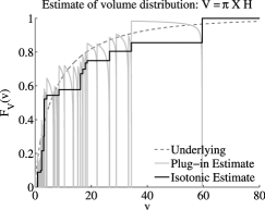
Figure 3: The estimates for the underlying distribution of the volume (given by the simulation in Section 6) for $n=50$ cylinders. The underlying distribution is given by the dashed grey line, the empirical plug-in estimate is given by the solid light grey line, and the isotonic estimate is given by the solid black line.

Briefly, the isotonic estimator is the (nonincreasing) function $\widehat{N}_{n}$ that minimizes

$$N\mapsto\int_{0}^{\infty}N(y)^{2}\,dy-2\int_{0}^{\infty}\widetilde{N}_{n}(y)N(y)\,dy$$ (14)

over all nonincreasing functions on $[0,\infty)$. It is tempting to “complete the square” and choose to minimize the function $\int(N(y)-\widetilde{N}_{n}(y))^{2}\,dy$ instead of (14), which should lead to the same solution since the added constant, $\int_{0}^{\infty}\widetilde{N}_{n}(y)^{2}\,dy$, does not depend on $N$. However, $\widetilde{N}_{n}$ is not square integrable, and so this added constant is infinite, making this problem ill defined. Therefore, we stick to minimizing (14).

To solve the minimization problem (continuous isotonic regression), we use Lemma 2 from Anevski and Soulier (2011) [see also Groeneboom and Jongbloed (2010)], where a characterization is given for the solution of our minimization problem. We begin by integrating the empirical estimator in (11) with respect to $t$, yielding

$$U_{n}(t) = \int_{u=0}^{t}\widetilde{N}_{n}(u)\,du$$

$$= \int_{u=0}^{t}\frac{1}{n}\sum_{i=1}^{n}\bigl{(}Z_{i}-q(H_{i};u)\bigr{)}^{-{1}/2}1_{[Z_{i}>q(H_{i};u)]}\,du.$$

Then, define $U_{n}^{*}$ to be the least concave majorant of $U_{n}$, enforcing monotonicity of its derivative. Finally, for $t\geq 0$, $\widehat{N}_{n}(t)=U_{n}^{*,r}(t)$ is the right-hand derivative of $U_{n}^{*}$ evaluated at $t$.

Sections 4 and 5 will consider the rates of convergence and asymptotic distributions for the plug-in estimators and the isotonic estimator in turn.

4 Asymptotic distributions of the plug-in estimators

There are a few assumptions on the observed variables that are required for the derivation of consistency and the various asymptotic distributions to hold.

Assumption 1.

$0<E_{g}[Z^{-{1}/2}]<\infty$. Equivalently, via (2) and (2), $0<E_{f}[\sqrt{X}]<\infty$.

Assumption 2.

$E_{g}[H^{5+\varepsilon}]<\infty$ for some $\varepsilon>0$.

Assumption 3.

$E_{g}[Z^{-{1}/2}H]<\infty$.

Under Assumptions 1, 2 and 3, the plug-in estimators for the distribution function of $H$, the quantities $N(t)$ for $X$, $R$, $S$ and $V$ (for fixed $t$), and the covariance in equations (10), (11) and (13), respectively, are consistent by the law of large numbers. From (2), (2) and (2) it follows that the random variables $Z^{-1/2}$, $HZ^{-1/2}$ and $[Z-q(H;t)]^{-1/2}1_{[Z>q(H;t)]}$ have infinite variances. This means that the standard (finite variance) central limit theorem cannot be used to derive relevant asymptotic distributions. The theorem below states a central limit result for random variables with infinite variances that will be needed in the sequel.

Theorem 1

Let $Y_{i}$, for $i=1,2,\ldots,$ be i.i.d. random variables. Denote the distribution of $Y_{i}$ by $K$ and define $\overline{Y_{n}}=\frac{1}{n}\sum_{i=1}^{n}Y_{i}$. If $E_{K}[Y_{i}]<\infty$ and $P_{K}(Y_{i}>c)\sim\frac{\kappa}{c^{2}}$ as $c\rightarrow\infty$ and $E_{K}[Y_{i}^{2}1_{[Y_{i}\in[0,c)]}]\sim\kappa\ln(c^{2})$, where $\kappa>0$ is a constant, then

$$\sqrt{\frac{n}{\ln(n)}}\bigl{(}\overline{Y_{n}}-E_{K}[Y_{i}]\bigr{)}\leadsto\mathcal{N}(0,\kappa).$$

We apply Theorem 4 from Chapter 9 of Chow and Teicher (1988). To this end, note that because $P_{K}(Y_{i}>c)\sim\frac{\kappa}{c^{2}}$ and $E_{K}[Y_{i}^{2}1_{[Y_{i}\in[0,c)]}]\sim\kappa\ln(c^{2})$, the following condition holds:

$$\lim_{c\rightarrow\infty}\frac{\int_{|y|>c}\,dK(y)}{({1}/{c^{2}})\int_{|y|<c}y^{2}\,dK(y)} = \lim_{c\rightarrow\infty}\frac{P(Y_{i}>c)}{({1}/{c^{2}})E_{K}[Y_{i}^{2}1_{[Y_{i}\in[0,c)]}]}$$

$$= \lim_{c\rightarrow\infty}\frac{\kappa}{\kappa\ln(c^{2})}=0.$$

Now, choose $c=\sqrt{n\ln(n)\kappa}$ and define $A_{n}=\frac{n}{B_{n}}\int_{|y|<B_{n}}y\,dK(y)$ and $B_{n}=\sup\{c\dvtx\frac{1}{c^{2}}\int_{|y|<c}y^{2}\,dK(y)\geq\frac{1}{n}\}$. This leads to $B_{n}\sim c$ and $A_{n}\sim\sqrt{\frac{n}{\ln(n)\kappa}}E_{K}[Y_{i}]$ for $n\rightarrow\infty$ since $E_{K}[Y_{i}]<\infty$. Consequently, the central limit theorem holds where, for $y\in\mathbb{R}$,

$$\lim_{n\rightarrow\infty}P\Biggl{(}\frac{1}{B_{n}}\sum_{i=1}^{n}Y_{i}-A_{n}<y\Biggr{)} = \lim_{n\rightarrow\infty}P\biggl{(}\sqrt{\frac{n}{\ln(n)\kappa}}\bigl{(}\overline{Y_{n}}-E_{K}[Y_{i}]\bigr{)}<y\biggr{)}$$

$$= \Phi(y),$$

where $\Phi$ is the CDF of the standard normal distribution.

4.1 Asymptotic distributions for the estimators of $N(t)$ and $F(t)$

Using Theorem 1, we derive the asymptotic distribution for estimators of $N(t)$ for the various choices of $q$ given in (4). We begin by defining the density function of the random variable $Z-q(H;t)$ as

$$\tau_{q}(z)=\tau_{q(\cdot;t)}(z)=\int_{h=0}^{\infty}g\bigl{(}z+q(h;t),h\bigr{)}\,dh.$$ (16)

Assumption 4.

$\tau_{q}^{\prime}$ is continuous and uniformly bounded by some $M<\infty$ in a right neighborhood of $0$.

If Assumption 4 holds, then (16) has the important property that for $\delta\downarrow 0$,

$$\int_{z=0}^{\delta}\tau_{q}(z)\,dz=\delta\tau_{q}(0)+o(\delta).$$ (17)

Theorem 2

Let $(Z_{i},H_{i})$ ($i=1,2\ldots$) be an i.i.d. sequence with density $g$ given in (2), $t\geq 0$ fixed, and let $q$ be any of the choices given by (4). Furthermore, let $\widetilde{N}_{n}$ be defined as in (11) and let Assumption 1 hold and Assumption 4 be satisfied for $q(\cdot;t)$ and $g$. Then

$$\sqrt{\frac{n}{\ln(n)}}\bigl{(}\widetilde{N}_{n}(t)-N(t)\bigr{)}\leadsto\mathcal{N}\bigl{(}0,\tau_{q}(0)\bigr{)}.$$ (18)

Define the i.i.d. sequence $Y_{1},Y_{2},\ldots$ by $Y_{i}=[Z_{i}-q(H_{i};t)]^{-{1}/2}\*1_{[Z_{i}>q(H_{i};t)]}$ for $i=1,2,\ldots$ with distribution function $K_{Y}$. Note that $\widetilde{N}_{n}(t)=n^{-1}\sum_{i=1}^{n}Y_{i}$ and $E[Y_{i}]=N(t)<\infty$ by Assumption 1 and (7). The tail probabilities of $Y_{i}$ behave like

$$P(Y_{i}>y) = P\biggl{(}\frac{1_{[Z_{i}>q(H_{i};t)]}}{\sqrt{Z_{i}-q(H_{i};t)}}>y\biggr{)}$$

$$= P\biggl{(}q(H_{i};t)<Z_{i}<\frac{1}{y^{2}}+q(H_{i};t)\biggr{)}$$

$$= \int_{h=0}^{\infty}\int_{z=q(h;t)}^{{1}/{y^{2}}+q(h;t)}g(z,h)\,dz\,dh$$

$$= \int_{h=0}^{\infty}\int_{z=0}^{{1}/{y^{2}}}g\bigl{(}z+q(h;t),h\bigr{)}\,dz\,dh$$

$$= \int_{z=0}^{{1}/{y^{2}}}\int_{h=0}^{\infty}g\bigl{(}z+q(h;t),h\bigr{)}\,dz\,dh$$

$$= \int_{z=0}^{{1}/{y^{2}}}\tau_{q}(z)\,dz=\frac{1}{y^{2}}\tau_{q}(0)+o\bigl{(}y^{-2}\bigr{)}.$$

Applying (17) as $y\rightarrow\infty$, we see that $\kappa=\tau_{q}(0)$ in Theorem 1. The expectation of $Y_{i}^{2}$ truncated at $c=\sqrt{n\ln(n)\kappa}$ is

$$E\bigl{[}Y_{i}^{2}1_{Y_{i}\in[0,c)}\bigr{]} = \int_{y=0}^{c}y^{2}\,dK_{Y}(y)$$

$$= \int_{y=0}^{c}2y\bigl{(}K_{Y}(c)-K_{Y}(y)\bigr{)}\,dy\sim\ln\bigl{(}c^{2}\bigr{)}\tau_{q}(0).$$

This relationship is proven in the supplemental article [McGarrity, Sietsma and Jongbloed (2014)]. Therefore, from Theorem 1 the result follows.

By Theorem 2, the asymptotic variances for the estimators $\widetilde{N}_{n}(t)$ based on the quantities $q$ for the squared radius, aspect ratio, surface area and volume, respectively, are given by

$$\displaystyle\int_{h=0}^{\infty}g(t,h)\,dh=g_{Z}(t),\qquad\int_{h=0}^{\infty}g\bigl{(}h^{2}t^{2},h\bigr{)}\,dh,$$

(20)

$$\displaystyle\int_{h=0}^{\infty}g\biggl{(}\biggl{[}\sqrt{\frac{h^{2}}{4}+\frac{t}{2\pi}}-\frac{h}{2}\biggr{]}^{2},h\biggr{)}\,dh\quad\mbox{and}\quad\int_{h=0}^{\infty}g\biggl{(}\frac{t}{\pi h},h\biggr{)}\,dh.$$

Note that for the squared radius, result (4.1) is not new. Since it is independent of height, this result is the same as the result stated in Theorem 2 by Groeneboom and Jongbloed (1995) for spherical particles in Wicksell’s problem. However, for the other quantities of interest, which require both the squared radius and the height of the cylinders, the result is different from what can be obtained by following Groeneboom and Jongbloed’s approach to the Wicksell problem. The asymptotic distributions of $\widetilde{N}_{n}(t)$ can be used to obtain the asymptotic distributions of the corresponding distribution functions of interest, evaluated at $t$. Note that for all choices of $q$ in (4), $\widetilde{N}_{n}(0)=\frac{1}{n}\sum_{i=1}^{n}Z_{i}^{-1/2}$ and $N(0)=E_{g}[Z^{-1/2}]=m_{G}^{-}=\pi/(2m_{F}^{+})$.

Corollary 1

Based on the estimators $\widetilde{N}_{n}(t)$ of Theorem 2, define $\widetilde{F}_{n}(t)=1-\widetilde{N}_{n}(t)/\widetilde{N}_{n}(0)$ as estimator for $F_{T}$ defined in (5). Then, under the conditions of Theorem 2, we have for $n\rightarrow\infty$

$$\sqrt{\frac{n}{\ln(n)}}\bigl{(}\widetilde{F}_{n}(t)-F(t)\bigr{)}\leadsto\mathcal{N}\biggl{(}0,\frac{N(0)^{2}\tau_{q}(0)+N(t)^{2}g_{Z}(0)}{N(0)^{4}}\biggr{)}.$$ (21)

The proof follows from Theorem 2 using Slutsky’s lemma.

4.2 Asymptotic distribution for the estimator of the covariance

Finding the asymptotic distribution of the covariance estimator is more complicated than for any single expectation estimator. Therefore, this asymptotic distribution is considered first and the results are then applied to the simpler estimators for the various expectations. From Assumption 2 the variance of $H$ is finite. Therefore, the standard central limit theorem for finite variance random variables holds for the sample mean of the $H_{i}$’s and we can define an approximating quantity for the covariance that depends only on the terms involving $Z^{-1/2}$ [compared to (13)]:

$$\widetilde{\sigma}_{n,\sqrt{X}H}=\frac{(\pi/2)E_{g}[H_{i}]}{n^{-1}\sum_{i=1}^{n}Z_{i}^{-{1}/2}}-\frac{\pi/2}{n^{-1}\sum_{i=1}^{n}Z_{i}^{-{1}/2}}\frac{\sum_{i=1}^{n}H_{i}Z_{i}^{-{1}/2}}{\sum_{i=1}^{n}Z_{i}^{-{1}/2}}.$$

Note that $\delta_{n}^{-1}(\hat{\sigma}_{n,\sqrt{X}H}-\widetilde{\sigma}_{n,\sqrt{X}H})\stackrel{{\scriptstyle P}}{{\rightarrow}}0$, where $\delta_{n}=\sqrt{\frac{\ln(n)}{n}}$. Hence, to derive the asymptotic distribution of $\delta_{n}^{-1}(\hat{\sigma}_{n,\sqrt{X}H}-{\sigma}_{n,\sqrt{X}H})$, it suffices to derive the asymptotic distribution of $\delta_{n}^{-1}(\widetilde{\sigma}_{n,\sqrt{X}H}-{\sigma}_{n,\sqrt{X}H})$. Considering this distribution, define the function $\phi\dvtx(0,\infty)^{2}\mapsto\mathbb{R}$ as

$$\phi(u,v)=\frac{\pi}{2}\biggl{(}\frac{E_{g}[H]}{u}-\frac{v}{u^{2}}\biggr{)}.$$

Moreover, define

$$T_{n}=\frac{1}{n}\sum_{i=1}^{n}\pmatrix{Z_{i}^{-{1}/2}\vspace*{3pt}\cr H_{i}Z_{i}^{-{1}/2}},$$ (22)

leading to $\widetilde{\sigma}_{n,\sqrt{X}H}=\phi(T_{n})$. In order to pin down the asymptotic variance of $\widetilde{\sigma}_{n,\sqrt{X}H}$, we need two more assumptions and the following lemma.

Assumption 5.

$\xi_{g}^{j}=\int_{h=0}^{\infty}h^{j}g(0,h)\,dh<\infty$ for $j=0,1,2$.

Assumption 6.

For some constant $K<\infty$, $|\frac{\partial}{\partial z}g(z,h)|\leq K$ for all $z,h\geq 0$.

Lemma 1

Let $T_{n}$ be as defined in (22). Assume that Assumptions 1, 2, 3, 5 and 6 hold, then

$$\delta_{n}^{-1}\bigl{(}T_{n}-E_{g}[T_{n}]\bigr{)}\leadsto\mathcal{N}(0,\Xi)\qquad\mbox{where }\Xi=\pmatrix{\xi_{g}^{0}&\xi_{g}^{1}\vspace*{3pt}\cr\xi_{g}^{1}&\xi_{g}^{2}}$$ (23)

and the entries in $\Xi$ can be formulated from (2) to yield

$$\xi_{g}^{j}=\int_{h=0}^{\infty}h^{j}g(0,h)\,dh=\frac{E_{f}[X^{-{1}/2}H^{j}]}{2E_{f}[X^{1/2}]}.$$ (24)

The proof of this lemma can be found in the supplemental article [McGarrity, Sietsma and Jongbloed (2014)]. We now apply the $\Delta$-method to the quantity $\phi(T_{n})$, which yields

$$\delta_{n}^{-1}(\widetilde{\sigma}_{n,\sqrt{X}H}-\sigma_{\sqrt{X}H})=\delta_{n}^{-1}\bigl{(}\phi(T_{n})-\phi\bigl{(}E_{g}[T_{n}]\bigr{)}\bigr{)}\leadsto\mathcal{N}\bigl{(}0,\nu^{2}\bigr{)},$$

where

$$\nu^{2}=\bigl{(}\nabla\phi\bigl{(}E_{g}[T_{n}]\bigr{)}\bigr{)}^{T}\Xi\bigl{(}\nabla\phi\bigl{(}E_{g}[T_{n}]\bigr{)}\bigr{)}$$

and

$$\nabla\phi(u,v)=\pmatrix{\displaystyle\frac{\partial}{\partial u}\phi(u,v)\vspace*{5pt}\cr\displaystyle\frac{\partial}{\partial v}\phi(u,v)}=\frac{\pi}{2}\frac{1}{u^{3}}\pmatrix{2v-E_{g}[H]u\vspace*{3pt}\cr-u}.$$

This provides $\nu^{2}$ in terms of the joint densities of the observable variables:

$$\nu^{2} = \biggl{(}\frac{\pi}{2}\biggr{)}^{2}E_{g}^{-4}\bigl{[}Z^{-{1}/2}\bigr{]}$$

$${}\times\biggl{\{}\xi_{g}^{0}\biggl{(}4\frac{E_{g}^{2}[Z^{-{1}/2}H]}{E_{g}^{2}[Z^{-{1}/2}]}-4\frac{E_{g}[Z^{-{1}/2}H]E_{g}[H]}{E_{g}[Z^{-{1}/2}]}+E_{g}^{2}[H]\biggr{)}$$

$$\hskip 89.5pt{}+2\xi_{g}^{1}\biggl{(}E_{g}[H]-\frac{E_{g}[Z^{-{1}/2}H]}{E_{g}[Z^{-{1}/2}]}\biggr{)}+\xi_{g}^{2}\biggr{\}}.$$

Given the cross-moment relationships in (2) and (24), $\nu^{2}$ can also be expressed in terms of the underlying joint distribution of the cylinder radii and heights:

$$\nu^{2} = \biggl{(}\frac{\pi}{2}\biggr{)}^{-2}E_{f}\bigl{[}X^{1/2}\bigr{]}$$

$${}\times\bigl{\{}E_{f}\bigl{[}X^{-{1}/2}\bigr{]}\bigl{(}4E_{f}^{2}\bigl{[}X^{1/2}\bigr{]}E^{2}_{f}[H]$$

$$\hskip 69.0pt{}-4E_{f}[H]E_{f}\bigl{[}X^{1/2}H\bigr{]}E_{f}\bigl{[}X^{1/2}\bigr{]}+E_{f}^{2}\bigl{[}X^{1/2}H\bigr{]}\bigr{)}$$

$$\hskip 16.0pt{}+2E_{f}\bigl{[}X^{-{1}/2}H\bigr{]}\bigl{(}E_{f}\bigl{[}X^{1/2}H\bigr{]}E_{f}\bigl{[}X^{1/2}\bigr{]}-E_{f}[H]E_{f}^{2}\bigl{[}X^{1/2}\bigr{]}\bigr{)}$$

$$\hskip 167.0pt{}+E_{f}\bigl{[}X^{-{1}/2}H^{2}\bigr{]}E_{f}^{2}\bigl{[}X^{1/2}\bigr{]}\bigr{\}}.$$

This proves the following theorem for the plug-in estimator for $\sigma_{\sqrt{X}H}$.

Theorem 3

Let $\sigma_{\sqrt{X}H}$ and $\hat{\sigma}_{n,\sqrt{X}H}$ be defined as in (2) and (13), respectively. Under the assumptions of Lemma 1, for $\nu^{2}$ defined in (4.2) and (4.2),

$$\sqrt{\frac{n}{\ln n}}(\hat{\sigma}_{n,\sqrt{X}H}-\sigma_{\sqrt{X}H})\leadsto\mathcal{N}\bigl{(}0,\nu^{2}\bigr{)}\qquad\mbox{as }n\rightarrow\infty.$$

4.3 Estimating the expectations

From (2) and (12), it is simple to verify that the various 3D quantities of interest are given by the 2D observable quantities with their empirical estimators given in Table 1.

Table 1: Expectations and empirical estimates of the 3D quantities of interest given as functions of the expectations and empirical estimates of the 2D observable quantities

Quantity of interest ($\bolds{T}$)	Expectation $\bolds{E_{f}[T]}$	Empirical estimator $\bolds{\widehat{E}_{f}[T]}$
Radius: $X^{1/2}$	$(\pi/2)(E_{g}[Z^{-{1/2}}])^{-1}$	$(\pi/2)((1/n)\sum_{i=1}^{n}Z_{i}^{-{1/2}})^{-1}$
Squared radius: $X$	$(2E_{g}[Z^{1/2}])(E_{g}[Z^{-{1/2}}])^{-1}$	$(2\sum_{i=1}^{n}Z_{i}^{{1/2}})(\sum_{i=1}^{n}Z_{i}^{-{1/2}})^{-1}$
Height: $H$	$(E_{g}[Z^{-{1/2}}H])(E_{g}[Z^{-{1/2}}])^{-1}$	$(\sum_{i=1}^{n}Z_{i}^{-{1/2}}H_{i})(\sum_{i=1}^{n}Z_{i}^{-{1/2}})^{-1}$
Volume: $\pi XH$	$(2\pi E_{g}[Z^{1/2}H])(E_{g}[Z^{-{1/2}}])^{-1}$	$(2\sum_{i=1}^{n}Z_{i}^{{1/2}}H_{i})(\sum_{i=1}^{n}Z_{i}^{-{1/2}})^{-1}$
Surface area:	$2\pi[(2E_{g}[Z^{1/2}])(E_{g}[Z^{-{1/2}}])^{-1}$	$2\pi[(2\sum_{i=1}^{n}Z_{i}^{{1/2}}H_{i})(\sum_{i=1}^{n}Z_{i}^{-{1/2}})^{-1}$
$2\pi(X+X^{1/2}H)$	${}+(\pi/2)E_{g}[H]$	${}+(\pi/2)(\sum_{i=1}^{n}H_{i})$
	${}\times(2E_{g}[Z^{-{1/2}}])^{-1}]$	${}\times(\sum_{i=1}^{n}Z_{i}^{-{1/2}})^{-1}]$
Aspect ratio:	$(\pi E_{g}[H^{-1}])(E_{g}[Z^{-{1/2}}])^{-1}$	$\pi(\sum_{i=1}^{n}H_{i}^{-1})(\sum_{i=1}^{n}Z_{i}^{-{1/2}})^{-1}$
$X^{1/2}H^{-1}$

Due to the dependence of the aspect ratio on $H^{-1}$, several more assumptions are required to continue this analysis. For brevity and simplicity, the expectation of the aspect ratio will not be considered any further.

To obtain the asymptotic distributions, Lemma 1 and the delta method can be used with the following assumption.

Assumption 7.

$E_{g}[Z^{1/2}H^{j}]<\infty$ and $E_{g}[(Z^{1/2}H^{j})^{2}]<\infty$, where $j=0,1$.

Under Assumption 7, the expectations can be treated as constants in the modified function $\phi$, as discussed for the expectation of the height in the previous section. The coefficients $s$ and $t$ for linearizing (22) are taken to be zero where appropriate. Then, the asymptotic variance for the estimation of the quantities of interest given above is listed in Table 2.

Table 2: Asymptotic variances $\nu_{g}^{2}$ from Corollary 2

Quantity of interest	Asymptotic variance $\bolds{\nu_{g}^{2}}$
Radius	$(\pi/2)^{2}\xi_{g}^{0}(E_{g}[Z^{-{1/2}}])^{-4}$
Squared radius	$4\xi_{g}^{0}(E_{g}[Z^{1/2}])^{2}(E_{g}[Z^{-{1/2}}])^{-4}$
Height	$\{\xi_{g}^{0}(E_{g}[Z^{-{1/2}}H])^{2}-2\xi_{g}^{1}E_{g}[Z^{-{1/2}}H]E_{g}[Z^{-{1/2}}]$
	${}+\xi_{g}^{2}(E_{g}[Z^{-{1/2}}])^{2}\}(E_{g}[Z^{-{1/2}}])^{-4}$
Volume	$4\pi^{2}\xi_{g}^{0}(E_{g}[Z^{1/2}H])^{2}(E_{g}[Z^{-{1/2}}])^{-4}$
Surface area	$\xi_{g}^{0}(4\pi E_{g}[Z^{1/2}]+\pi^{2}E_{g}[H])^{2}(E_{g}[Z^{-{1/2}}])^{-4}$

This leads to the following corollary to Theorem 3.

Corollary 2

Let $E_{f}[T]$ and $\widehat{E}_{f}[T]$ be defined as in Table 1, where $T$ is any of the quantities of interest listed in Table 1. Under the assumptions of Lemma 1 and Assumption 7, for $\nu_{g}^{2}$ as defined in Table 2,

$$\sqrt{\frac{n}{\ln(n)}}\bigl{(}\widehat{E}_{f}[T]-E_{f}[T]\bigr{)}\leadsto\mathcal{N}\bigl{(}0,\nu_{g}^{2}\bigr{)}\qquad\mbox{as }n\rightarrow\infty.$$

Theorem 3 and Corollary 2 show that the expectations of the quantities of interest can be estimated consistently with a rate of $\sqrt{\ln(n)/n}$. These results can be used to obtain the 95% confidence intervals for the unknown expectations being estimated by $\widehat{E}_{f}[T]$:

$$\widehat{E}_{f}[T]\pm 1.96\nu_{g}\sqrt{\frac{\ln(n)}{n}}.$$ (27)

For a discussion on the small sample properties and coverage probability of the confidence intervals, see Chapter 4 of McGarrity (2013) and the supplemental article [McGarrity, Sietsma and Jongbloed (2014)].

4.4 Asymptotic distribution for the estimator of the height distribution

Consider the plug-in estimator for the distribution function of heights, given in (10). As mentioned before, under Assumption 2, the law of large numbers immediately gives that $\widehat{F}_{H,n}(h)\stackrel{{\scriptstyle P}}{{\rightarrow}}F_{H}(h)$ as $n\rightarrow\infty$. The asymptotic distribution is given in the theorem below.

Theorem 4

Consider $F_{H}(h)$ and $\widehat{F}_{H,n}(h)$ as given in (3) and (10), respectively. Under Assumptions 1 and 5,

$$\sqrt{\frac{n}{\ln n}}\bigl{(}\widehat{F}_{H,n}(h)-F_{H}(h)\bigr{)}\leadsto\mathcal{N}\bigl{(}0,\nu^{2}\bigr{)},$$

where $\nu^{2}=(m_{G}^{-})^{-2}(F_{H}(h)\int_{h}^{\infty}g(0,y)\,dy+(1-F_{H}(h))\int_{0}^{h}g(0,y)\,dy)$.

Consider the random vectors

$$T_{n}=\frac{1}{n}\sum_{i=1}^{n}\pmatrix{Z_{i}^{-{1}/2}\vspace*{3pt}\cr Z_{i}^{-{1}/2}1_{[H_{i}<h]}}$$

with

$$E[T_{n}]=\pmatrix{m_{G}^{-}\vspace*{3pt}\cr\displaystyle\int_{z=0}^{\infty}\int_{y=0}^{h}z^{-{1}/2}g(z,y)\,dy\,dz}.$$

For $T_{n}$ it is shown in the supplemental article [McGarrity, Sietsma and Jongbloed (2014)] that

$$\sqrt{\frac{n}{\ln n}}\bigl{(}T_{n}-E[T_{n}]\bigr{)}\leadsto{\mathcal{N}}(0,\Xi),$$ (28)

where the entries of $\Xi$ are given by $\xi_{12}=\xi_{21}=\xi_{22}=\int_{y=0}^{h}g(0,y)\,dy$ and $\xi_{11}=g_{Z}(0)$. The result follows by applying the $\Delta$-method to the function $\phi(u,v)=v/u$ at $T_{n}$, yielding asymptotic normality with variance $\nu^{2}$.

The estimator for the distribution of the heights given in (10) accounts for any dependence between the radius and height of the cylinders. Any correlation that might exist will lead to the height observations being biased like the rectangle half-width observations due to the larger cylinders being more likely to be intersected by the cut plane. However, if the heights are known to be independent from the cylinder radius, then the biasing in the problem has no consequences for the distribution of observable heights and we may simply take the empirical distribution of the observed heights to be the estimate of the actual distribution:

$$\widehat{F}_{H}(h)=\frac{1}{n}\sum_{i=1}^{n}1_{[H_{i}\leq h]}.$$

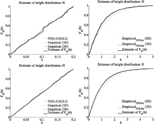
Figure 4: The upper and lower figures show the estimate of $F_{H}(h)$ for $n=500$ and $n=5000$ cylinders, respectively. The dark grey lines show the 3D empirical distributions of the cylinder heights. The light grey lines show the 2D empirical distributions. The black lines show the estimates of the 3D distributions as calculated from (10). The left images are of cylinders whose height and radii are uncorrelated and the underlying distribution of the height is shown by the grey dot-dashed line. The right images are of cylinders whose height and radii are correlated.

This estimator has a rate of convergence of $1/\sqrt{n}$. Figure 4 shows the effect of the rate of convergence for the estimation procedure. Focusing on the left images, the upper image shows the 2D (light grey line) and 3D (dark grey line) empirical distributions for the heights of 500 uncorrelated (radii and cylinder heights), uniformly distributed cylinders. The bottom image shows the same for 5000 cylinders. The black solid line shows the estimation of the 3D distribution as calculated from (10). The empirical distribution is a better choice than (10) in this case because it has the faster rate of convergence. Contrarily, focusing on the right images where there is a nonzero correlation between the radii and heights of the cylinders, the biasing in the 2D distribution (light grey lines compared to the dark grey line for the 3D empirical distribution) is clear. In this case, the estimator from (10) is necessary to accurately estimate the underlying 3D distribution.

5 Asymptotic distributions of the isotonic estimators

In this section we study the consistency and asymptotic behavior of the isotonic estimators, $\widehat{N}_{n}$, as described in Section 3. To do so requires one further assumption.

Assumption 8.

$\int_{0}^{\infty}N(t)\,dt<\infty$.

Theorem 5

Suppose $t\geq 0$ and $F_{T}$ from (5) has a density $f$ that is strictly positive and continuous in a neighborhood of $t$ (a right neighborhood if $t=0$) and that $q(h;t)$ is defined as in (4). Further, suppose that Assumptions 1, 4 and 8 hold. Then,

$$\sqrt{\frac{n}{\ln n}}\bigl{(}\widehat{N}_{n}(t)-N(t)\bigr{)}\leadsto\mathcal{N}\biggl{(}0,\frac{1}{2}\tau_{q}(0)\biggr{)}$$ (29)

as $n\rightarrow\infty$.

The proof of this theorem can be found in the supplemental article [McGarrity, Sietsma and Jongbloed (2014)]. The striking difference with Theorem 2 is the factor $1/2$ in the asymptotic variance. This means that enforcing monotonicity in the estimator improves on the empirical estimator because the resulting estimator satisfies the natural monotonicity constraint. Moreover, it also leads to a more accurate estimator asymptotically.

Analogous to Corollary 1, we have the following corollary.

Corollary 3

Suppose that $q(h;t)>0$ for all $h$ and $t>0$, and that $F_{T}(t)$ has a density $f$ which is strictly positive at $t$ and continuous in a neighborhood of $t$. Then, under the assumptions of Theorem 5,

$$\qquad\sqrt{\frac{n}{\ln(n)}}\biggl{(}1-\frac{\widehat{N}_{n}(t)}{\widehat{N}_{n}(0)}-F_{T}(t)\biggr{)}\leadsto\mathcal{N}\biggl{(}0,\frac{N(0)^{2}\tau_{q}(0)+N(t)^{2}g_{Z}(0)}{2N(0)^{4}}\biggr{)}$$ (30)

as $n\rightarrow\infty$.

The proof of this corollary is analogous to the proof of Corollary 2 given in Groeneboom and Jongbloed (1995), in our case applying Theorem 5 from above. Recall that consistency at zero follows from Lemma 1 in the supplemental article [McGarrity, Sietsma and Jongbloed (2014)].

6 Simulation

To validate the model and estimators, we implemented a simulation where we work directly with the distributions of $X$ and $H$ to calculate the distributions of $Z$ and $H$ for the rectangles, as well as the other quantities of interest. To start, $X$ is taken to be Gamma(3) distributed and $H$, given $X=x$, is triangularly distributed on $[0,x]$:

$$f_{X}(x) = \tfrac{1}2x^{2}e^{-x},\qquad x\geq 0,$$

$$f_{H|X}(h|x) = \frac{2}{x^{2}}(x-h),\qquad h\in(0,x).$$

From the above, marginal and conditional densities of the observable quantities can be calculated:

$$g_{Z}(z) = \tfrac{4}{15}\bigl{(}z^{2}+z+\tfrac{3}4\bigr{)}e^{-z},\qquad z\geq 0,$$

$$g_{H|Z}(h|z) = \frac{2({1}/2+z-h)}{(z^{2}+z+{3}/4)}1_{[0<h<z]}$$

$${}+\frac{2[({1}/2+z-h)I_{G}({1}/2,(h-z))+\sqrt{h-z}e^{-(h-z)}]}{\sqrt{\pi}(z^{2}+z+{3}/4)}1_{[h>z]},$$

where $I_{G}(m,x)=\int_{t=x}^{\infty}t^{m-1}e^{-t}\,dt$ is the incomplete Gamma function. From the joint densities, the underlying distributions for the various quantities of interest ($V$, $S$ and $R$) can be calculated. As an example, the distribution function for the volume is as follows:

$$\qquad F_{V}(v)=1-\biggl{[}1+\sqrt{\frac{v}{\pi}}-\frac{v}{2\pi}+\frac{1}{2}\biggl{(}\frac{v}{\pi}\biggr{)}^{3/2}\biggr{]}e^{-\sqrt{{v/\pi}}}+\frac{v^{2}}{2\pi^{2}}Ei\biggl{(}\sqrt{\frac{v}{\pi}}\biggr{)},$$ (33)

where $Ei(x)=\int_{u=x}^{\infty}e^{-u}u^{-1}\,du$ is the exponential integral. For this simulation, we draw $n$ observations from the marginal density $g_{Z}$. For each observation from $Z$, a corresponding height observation is drawn from the conditional density $g_{H|Z}$ to form the 2D observations $(Z_{1},H_{1}),\ldots,(Z_{n},H_{n})$ for the $n$ rectangles. From these observations it is possible to estimate the various quantities of interest for the cylinder, beginning with the covariance between the cylinder height and radius.

Table 3: Results of the covariance estimation for the simulation. $n$ is the number of observed rectangles on the cut plane. $\hat{\sigma}_{n,\sqrt{X}H}$ is the covariance estimate given in (13). $\hat{\nu}_{g}^{2}$ is the asymptotic variance determined from a single simulation run based on (4.2) using the empirical means as estimates for the expectations in the equation. The fourth column gives half the width of the constructed 95% confidence interval for the covariance. The fifth column gives the empirical mean from 1000 simulation runs of the covariance estimate

Covariance estimator and the asymptotic variance
$\bolds{n}$	$\bolds{\hat{\sigma}_{n,\sqrt{X}H}}$	$\bolds{\hat{\nu}_{g}^{2}}$	$\bolds{1.96\sqrt{\frac{\ln n}{n}}\hat{\nu}_{g}}$	$\bolds{\frac{1}{1000}\sum_{i=1}^{1000}\hat{\sigma}_{i,n,\sqrt{X}H}}$
,00050	$0.424$	$1.11$	$0.58$	$0.266$
500	$0.331$	$1.12$	$0.23$	$0.277$
5000	$0.262$	$1.58$	$0.10$	$0.277$
50,000	$0.273$	$1.53$	$0.04$	$0.276$
,000$\infty$	$0.277$	$1.50$	$-$	$0.277$

Table 3 shows the results for the estimation of the covariance of $\sqrt{X}$ and $H$ as calculated from the 2D observations. The first column indicates the number of observed rectangles on the cut plane. For $n=\infty$, the true underlying covariance and asymptotic variance are given. For this simulation, the underlying covariance, as calculated from (2) and (6), is $0.277$, and the true underyling asymptotic variance, as calculated from (4.2) and (6), is $1.50$. The second column gives the estimates of the covariance for a single simulation run. The third column gives the estimate of the asymptotic variance for the covariance estimator for a single simulation run. The asymptotic variance was estimated from the empirical means for the expectations in (4.2) and by using the following estimator for (24):

$$\hat{\xi}_{g}^{j}=\frac{1}{b_{n}n}\sum_{i=1}^{n}H_{i}^{j}1_{[0,b_{n}]}(Z_{i}),$$ (34)

where $b_{n}\sim n^{-1/3}$ is a cutoff value for approximating $z=0$ and can be shown to have an optimal vanishing rate for the MSE of $n^{-2/3}$ (see Chapter 3 of McGarrity (2013) for details of the MSE and the supplemental article [McGarrity, Sietsma and Jongbloed (2014)] for a discussion on the affects of the choice of bandwidth). The fourth column gives the half-widths of the constructed 95% confidence interval for the covariance using the estimators for the covariance.

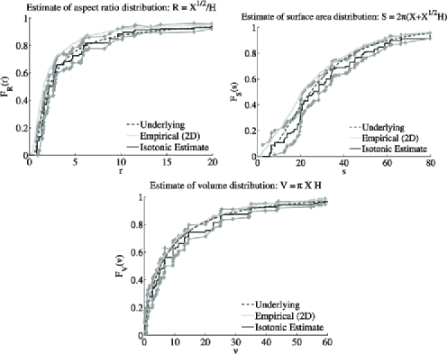
Figure 5: Plots of the cumulative distribution functions for the aspect ratio, $R$, surface area, $S$, and volume, $V$, for $n=500$ observations of $(Z,H)$ drawn from the 2D distributions in (6). In all figures, the dashed dark grey line gives the underlying distribution, the light grey line gives the empirical distribution based on the 2D observations $(Z,H)$, and the black line gives the isotonic estimation of the distribution of the quantity of interest based on the 2D observations. The grey diamonds give approximate 95% point-wise confidence sets for the isotonic estimator.

The final column shows the empirical mean over 1000 simulation runs of the covariance estimate using the 2D observations. The results behave as expected. While the single simulation runs at small $n$ give large values for the covariance estimate, the true covariance falls within the constructed 95% confidence interval. As $n$ increases, the estimated covariance approaches the true covariance. For the mean of 1000 simulation runs, we see that the estimated value of the covariance is much closer to the expected value, even for small $n$. This demonstrates the consistency and unbiased nature of the estimator.

It is also possible to estimate the underlying distribution functions, such as that given in (33), and compare the empirical distribution function of the quantities of interest also based on the 2D observations $(Z_{1},H_{1}),\ldots,(Z_{n},H_{n})$ treated as if they were distributed as the $(X,H)$. This means, for example, that for (33), $V_{i}=\pi Z_{i}H_{i}$. This is done because often only 2D data is accessible and has often been justified as a reasonable approximation for the 3D data. In the case of the squared radius, including the 2D data in this way emphasizes the bias inherent in the observations. For the volume, surface area and aspect ratio, the bias still exists. The question is whether the proposed estimators provide a better estimate than using the 2D data straight up, and, compared to the confidence intervals, it would seem that indeed it is.

Applying both the empirical and isotonic estimation procedures to the generated data sets leads to the results for the estimation of the aspect ratio (left), the surface area (middle) and the volume (right) displayed in Figure 5. The underlying distribution is given by the dashed dark grey curve. The empirical distribution based on the 2D observations [as if the $(Z,H)$ were distributed as the $(X,H)$] is given by the light grey curve. The isotonic estimate of the distribution of the quantity of interest based on the 2D observations is given by the black curve. The 95% point-wise confidence sets for the isotonic estimator are given by the grey diamonds.

The point-wise confidence sets are calculated from the results of Corrollary 3. To obtain an estimate of the asymptotic variance $\nu_{g}$ given in (30), only the function $\tau_{q}(0)=\int_{h=0}^{\infty}g(q(h;t),h)\,dh$ needs yet to be estimated. The estimates for $N(0)$ and $N(t)$ can be obtained from the isotonic estimates described in Section 3. The function $g_{Z}(0)=\xi_{g}^{0}$ and can be estimated by (34). Following the same idea as this estimator, and without going into the asymptotic behavior, we can estimate $\tau_{q}(0)$ consistently as

$$\hat{\tau}_{q}(0)=\frac{1}{2b_{n}n}\sum_{i=1}^{n}1_{[-b_{n},b_{n}]}\bigl{(}Z_{i}-q(H_{i};t)\bigr{)}.$$

The underlying distribution is mostly within the 95% point-wise confidence sets indicating that the estimator is reasonable and can be used in practice.

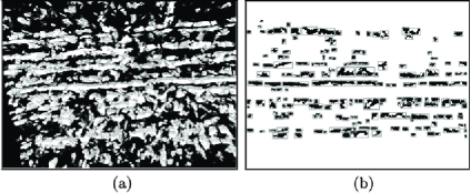
Figure 6: Figure (a) shows a view of the 3D reconstruction of the banded microstructure from the serial sectioned images. Figure (b) shows the bounding boxes around the features of interest (heretofore referred to as rectangles and cylinders for the 2D and 3D objects, resp.) in the microstructure.

7 Application of the model to real microstructures

The model and estimation procedures are now applied to the banded steel microstructure shown in Figure 1. To obtain 3D information about the microstructure, the material was serial sectioned, providing images approximately every 2 µm into a depth of about 90 µm. For details on the experimental procedure see McGarrity, Sietsma and Jongbloed (2012b). The optical images were processed with dilation and closing image operations on binary thresholds. The serial sectioned images were combined to form a single 3D object, shown in Figure 6(a), and the bounding boxes, that is the smallest box that contains all voxels of the object being considered, around the 3D features of interest (heretofore referred to as cylinders) were found using the 3D analysis function in Fiji [Bolte and Cordelières (2006)]. From Figure 6(a) it is clear that the 3D data is incomplete. The sectioning depth was not sufficient to observe a cylinder in its entirety. This gives a clear indication of why using this model to estimate the distributions of the quantities of interest is so important. Using even one of the section images, like the one shown in Figure 6(b), can provide a reasonable estimate for the underlying 3D distribution that is costly to obtain directly. Figure 6(b) shows rectangles around the 2D features of interest. These are the smallest rectangles to fully contain the objects of interest and are called bounding boxes. These rectangles were found using Fiji software [Rasband (1997–2009)] and yield the observed data pairs $(Z,H)$ used in the estimation procedures. For a discussion on using bounding boxes to represent the rectangles and how it affects the results of the model, see Chapter 6 of McGarrity (2013).

=200pt Moment and covariance estimates ($\bolds{n=179}$) Quantity 2D estimate $\bolds{{\pm}1.96\sqrt{\frac{\ln n}{n}}\hat{\nu}_{g}}$ $E[\sqrt{X}]$ $10.55\pm 2.30$ µm000 $E[X]$ $125\pm 27$ µm²00 $E[H]$ $8.72\pm 0.56$ µm00 $E[S]$ $1434\pm 332$ µm²00 $E[V]$ $4370\pm 950$ µm³00 $\sigma_{\sqrt{X}H}$ 00.$11.1\pm 25.6<0$ µm²

Table 4: Results for the moment and covariance estimates of the microstructure data with 179 rectangle observations. The first column gives the estimated quantity. The second gives the estimate of that quantity with the half-widths of the constructed 95% confidence intervals using the estimates for the asymptotic variance

Table 4 gives the 2D estimates for the moments and covariance, and the half-widths of their constructed 95% confidence intervals. The second column of the table gives the estimates using (12) and (13) for the moments and covariance based on a single 2D estimate for the asymptotic variances of the moments from Table 2. For the covariance, the estimates for the asymptotic variance come from (4.2).

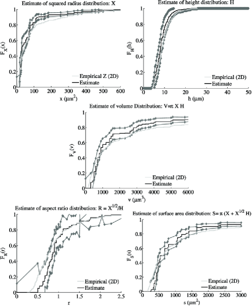
Figure 7: Results of the model and estimation procedures applied to the microstructure shown in Figure 6. The number of observations is $n=179$. The light grey lines are the estimates obtained by treating the squared half-width and height of the bounding box as if it were the squared radius and height of the cylinder. The black lines give the isotonic estimations of the underlying distribution functions of the quantities of interest given the 2D observations. The grey diamonds give the asymptotic 95% point-wise confidence sets for the isotonic estimates.

Using the 2D data set from any single slice of the serial sectioning, we can apply the model and estimation procedures to find the CDFs of the various quantities of interest. Figure 7 shows the results of the estimation procedures. The upper left plot shows the results for the isotonic estimation of the squared radius distribution. The upper right plot shows the plug-in estimation results for the height distribution. The middle plot and the lower left and right plots show the results for the isotonic estimation of the distributions for the volume, aspect ratio and surface area, respectively. In all plots, the light grey lines show the empirical estimates obtained by treating the rectangle squared half-width and height as if they were the squared radius and height of the cylinder. The black lines are the isotonic estimation results for the underlying distribution functions of the quantities of interest given the 2D observations. The grey diamonds give the asymptotic point-wise confidence sets for the isotonic estimates of $F_{T}$ taken at the values of $t$ corresponding to the 2D observations. These bands are calculated from the results of Corollary 3 and Theorem 4. For the asymptotic variance of the height distribution, the estimator $\widehat{F}_{H,n}$ is used. An estimator for the integrals again follows the same idea as the estimator for $\xi_{g}^{0}$, and, without considering the asymptotic behavior, we obtain

$$\frac{1}{b_{n}n}\sum_{i=1}^{n}1_{[0,b_{n}]}(Z_{i})1_{[h,\infty]}(H_{i}) \rightarrow \int_{y=h}^{\infty}g(0,y)\,dy,$$

$$\frac{1}{b_{n}n}\sum_{i=1}^{n}1_{[0,b_{n}]}(Z_{i})1_{[0,h]}(H_{i}) \rightarrow \int_{y=0}^{h}g(0,y)\,dy.$$

As can be seen from the plots in Figure 7, using the empirical 2D distributions tends to overestimate the small values and underestimate the large values of the quantities of interest. The 2D empirical distributions do not provide a reasonable picture for the distribution of the 3D quantities of interest. The exception to that, of course, is the height distribution. Due to the potential correlation between the radius and height of the cylinders, shown by a nonzero covariance between them in Table 4, there appears to be a small bias in the 2D observations, leading to a slight underrepresentation of the larger height values, yet it is still encompassed within the point-wise confidence sets. The results of the estimates for the covariance of the cylinder radius and height, the estimates for the various moments and the isotonic estimates for the CDFs of the 3D quantities of interest provide a glimpse into the microstructure that cannot be reliably obtained from the serial sectioned data.

8 Discussion

Often, it is difficult to know about the full 3D nature of the material or object being studied. The methods available to obtain 3D data about a material tend to be expensive in terms of resources and time, destructive and limited to small length scales. For instance, the total attained depth from several weeks of serial sectioning was about 90 µm for the microstructures shown in this work, while many of the cylinders are seen to be significantly larger than that. The serial sectioning is not enough to view a cylinder in its entirety through the depth of the sectioning. Therefore, in industry in particular, most information about a material is based upon 2D observations, which in many cases is insufficient. Stereology was developed to address this issue and to find ways to extract information about the 3D nature from the 2D observations. However, in order to be able to do this, certain assumptions must be made about the objects being studied. In the case of the Oriented Cylinder Model introduced in this work, the assumptions are that the objects in the material can be represented by circular cylinders whose axes of symmetry are all oriented in the same direction and that the cut through the material is along that axis. It is also assumed that the cylinders are uniformly distributed throughout the material. While this model is simple and the assumptions are somewhat ideal, our observations suggest that this is a reasonable starting point upon which more complex models can be built. The Oriented Cylinder Model provides insight into the material that has, until now, been lacking.

Assuming the model assumptions are reasonable, estimators are used to obtain estimates of the unknown underlying distributions of various quantities of interest. Since so little is known about the material studied in this work, nonparametric estimators were chosen rather than parametric ones since not enough is known about the material to assume a specific distribution. While parametric estimators will have a better rate of convergence and smaller variance, the difference is of order $\sqrt{\ln(n)}$. The flexibility afforded by the nonparametric model makes up for this difference.

The results presented especially for the microstructure data in Section 7 are informative, given how little information is available for the 3D nature of the material. However, there are several considerations, particularly inherent to processing the images, that have not been considered in this particular work. Edge effects are not accounted for in this analysis. The cylinders are considered to be completely inbounds of the observation window. However, it is possible that cylinders ending at the edge of the image continue beyond and this is not accounted for in this analysis. While edge effects can be eliminated from the simulation results presented in Section 6, they cannot reasonably be ignored for the microstructure. Features of interest like microstructural bands often deviate from perfect cylinders and are not observable as perfect rectangles. This leads to challenges in defining the dimensions of the observed rectangle. In this work, the bounding box around the feature of interest was taken as the rectangle. However, using the bounding box leads to overestimation of the heights and squared radii, though the significance of this overestimation is not immediately known. Determining an object of interest in an image is often done through pixel connectivity. Even though the images have undergone morphological processing, as described in McGarrity, Sietsma and Jongbloed (2012a), it is not always possible to preserve the true connectivity of the objects. How this affects the outcome of the estimation under the model assumptions is also not immediately clear. These issues are important to consider, but are beyond the scope of this particular work.

Despite these issues, and the simplicity of the model, the estimated distributions for the 3D quantities of interest are practicable representations of the underlying distributions. As a first step toward understanding and modeling a full 3D microstructure, this work provides a solid starting point and a reasonable approximation to what is often not directly observable.

Appendix: Relationships for the quantities of interest

First, define the quantity of interest, squared radius, aspect ratio, surface area or volume, as $t$. Let $(u,h)$ be the observed pair of variables. For a fixed $h>0$ we can define $t=p(h;u)$ for each quantity of interest. In (4) the inverse of $p(h;u)$ is defined as $u=q(h;t)$. These can each be calculated as follows:

$$p(h;u) = \left\{\matrix{u&\mbox{(squared radius)}&t\vspace*{3pt}\cr\displaystyle\frac{\sqrt{u}}{h}&\mbox{(aspect ratio)}&(ht)^{2}\vspace*{3pt}\cr 2\pi(u+h\sqrt{u})&\mbox{(surface area)}&\displaystyle{\biggl{[}\sqrt{\frac{h^{2}}{4}+\frac{t}{2\pi}}-\frac{h}{2}\biggr{]}^{2}}\vspace*{3pt}\cr\pi hu&\mbox{(volume)}&\displaystyle{\frac{t}{\pi h}}}\right\}$$

$$= q(h;t).$$

It is important to note for all choices of $p(h;u)$ and $q(h;t)$ that $p(h;q(h;t))=t$ and $q(h;p(h;u))=u$.

The derivative of these functions with respect to the second argument is also important. Denoting this partial derivative of $p$ with respect to $u$ by $\dot{p}$ and the partial derivative of $q$ with respect to $t$ by $\dot{q}$ results in

$$\dot{p}(h;u) = \left\{\matrix{1&\mbox{(squared radius)}&1\vspace*{3pt}\cr\displaystyle\frac{1}{2h\sqrt{u}}&\mbox{(aspect ratio)}&2h^{2}t\vspace*{3pt}\cr\displaystyle 2\pi\biggl{(}1+\frac{h}{2\sqrt{u}}\biggr{)}&\mbox{(surface area)}&\displaystyle\frac{1}{2\pi}\biggl{(}1-\frac{h}{2\sqrt{{h^{2}}/{4}+{t}/{2\pi}}}\biggr{)}\vspace*{3pt}\cr\pi h&\mbox{(volume)}&\displaystyle\frac{1}{\pi h}}\right\}$$

$$= \dot{q}(h;t).$$

Considering the relationship between $\dot{p}$ and $\dot{q}$ and using the linear approximation of $q$ near $t$ yields

$$\dot{p}\bigl{(}h;q(h;t)\bigr{)} = \lim_{\varepsilon\downarrow 0}\frac{p(h;q(h;t+\varepsilon/\dot{q}(h;t)))-p(h;q(h;t))}{\varepsilon}$$

$$= \lim_{\varepsilon\downarrow 0}\frac{t+\varepsilon/\dot{q}(h;t)-t}{\varepsilon}$$

$$= \frac{1}{\dot{q}(h;t)}.$$

Finally, note that $y>q(h;t)$ if and only if $t<p(h;y)$. Recall the expression for $W_{n}$ can be written in terms of the function $\phi_{n,v}$. We can use the substitution $u=q(h;y)$ in the definition of $\phi_{n,v}$ and obtain, for $z$ and $h$ fixed,

$$\phi_{n,v}(z,h) = \int_{y=t}^{(t+\delta_{n}v)\wedge p(h;z)}\bigl{[}z-q(h;y)\bigr{]}^{-{1}/2}\,dy$$

$$= \int_{u=q(h;t)}^{q(h;t+\delta_{n}v)\wedge z}(z-u)^{-{1}/2}\dot{p}(h;u)\,du.$$

References

- Andersen, Holme and Marioara (2008) {barticle}[pbm] \bauthor\bsnmAndersen, \bfnmSigmund J.\binitsS. J., \bauthor\bsnmHolme, \bfnmBørge\binitsB. and \bauthor\bsnmMarioara, \bfnmCalin D.\binitsC. D. (\byear2008). \btitleQuantification of small, convex particles by TEM. \bjournalUltramicroscopy \bvolume108 \bpages750–762. \biddoi=10.1016/j.ultramic.2007.12.001, issn=0304-3991, pii=S0304-3991(07)00263-X, pmid=18276077 \bptokimsref\endbibitem
- Anevski and Soulier (2011) {barticle}[mr] \bauthor\bsnmAnevski, \bfnmDragi\binitsD. and \bauthor\bsnmSoulier, \bfnmPhilippe\binitsP. (\byear2011). \btitleMonotone spectral density estimation. \bjournalAnn. Statist. \bvolume39 \bpages418–438. \biddoi=10.1214/10-AOS804, issn=0090-5364, mr=2797852 \bptokimsref\endbibitem
- Bolte and Cordelières (2006) {barticle}[mr] \bauthor\bsnmBolte, \bfnmS.\binitsS. and \bauthor\bsnmCordelières, \bfnmF. P.\binitsF. P. (\byear2006). \btitleA guided tour into subcellular colocalization analysis in light microscopy. \bjournalJ. Microsc. \bvolume224 \bpages213–232. \biddoi=10.1111/j.1365-2818.2006.01706.x, issn=0022-2720, mr=2312809 \bptokimsref\endbibitem
- Chow and Teicher (1988) {bbook}[mr] \bauthor\bsnmChow, \bfnmYuan Shih\binitsY. S. and \bauthor\bsnmTeicher, \bfnmHenry\binitsH. (\byear1988). \btitleProbability Theory: Independence, Interchangeability, Martingales, \bedition2nd ed. \bpublisherSpringer, \blocationNew York. \biddoi=10.1007/978-1-4684-0504-0, mr=0953964 \bptokimsref\endbibitem
- Cruz-Orive and Weibel (1990) {barticle}[author] \bauthor\bsnmCruz-Orive, \bfnmLuis M.\binitsL. M. and \bauthor\bsnmWeibel, \bfnmEwald R.\binitsE. R. (\byear1990). \btitleRecent stereological methods for cell biology: A brief survey. \bjournalAmerican Journal of Physiology \bvolume258 \bpagesL148–L156. \bptokimsref\endbibitem
- Cruz-Orive et al. (1985) {barticle}[mr] \bauthor\bsnmCruz-Orive, \bfnmL.-M.\binitsL.-M., \bauthor\bsnmHoppeler, \bfnmH.\binitsH., \bauthor\bsnmMathieu, \bfnmO.\binitsO. and \bauthor\bsnmWeibel, \bfnmE. R.\binitsE. R. (\byear1985). \btitleStereological analysis of anisotropic structures using directional statistics. \bjournalJ. Roy. Statist. Soc. Ser. C \bvolume34 \bpages14–32. \biddoi=10.2307/2347881, issn=0035-9254, mr=0793336 \bptokimsref\endbibitem
- Fullman (1953) {barticle}[author] \bauthor\bsnmFullman, \bfnmR. L.\binitsR. L. (\byear1953). \btitleMeasurement of particle sizes in opaque bodies. \bjournalTransactions AIME (Journal of Metals) \bvolume197 \bpages447–452. \bptokimsref\endbibitem
- Giumelli, Militzer and Hawbolt (1999) {barticle}[author] \bauthor\bsnmGiumelli, \bfnmA. K.\binitsA. K., \bauthor\bsnmMilitzer, \bfnmM.\binitsM. and \bauthor\bsnmHawbolt, \bfnmE. B.\binitsE. B. (\byear1999). \btitleAnalysis of the austenite grain size distribution in plain carbon steels. \bjournalISIJ International \bvolume39 \bpages271–280. \bptokimsref\endbibitem
- Groeneboom and Jongbloed (1995) {barticle}[mr] \bauthor\bsnmGroeneboom, \bfnmPiet\binitsP. and \bauthor\bsnmJongbloed, \bfnmGeurt\binitsG. (\byear1995). \btitleIsotonic estimation and rates of convergence in Wicksell’s problem. \bjournalAnn. Statist. \bvolume23 \bpages1518–1542. \biddoi=10.1214/aos/1176324310, issn=0090-5364, mr=1370294 \bptokimsref\endbibitem
- Groeneboom and Jongbloed (2010) {barticle}[mr] \bauthor\bsnmGroeneboom, \bfnmPiet\binitsP. and \bauthor\bsnmJongbloed, \bfnmGeurt\binitsG. (\byear2010). \btitleGeneralized continuous isotonic regression. \bjournalStatist. Probab. Lett. \bvolume80 \bpages248–253. \biddoi=10.1016/j.spl.2009.10.014, issn=0167-7152, mr=2575453 \bptnotecheck year \bptokimsref\endbibitem
- Hall and Smith (1988) {barticle}[mr] \bauthor\bsnmHall, \bfnmPeter\binitsP. and \bauthor\bsnmSmith, \bfnmRichard L.\binitsR. L. (\byear1988). \btitleThe kernel method for unfolding sphere size distributions. \bjournalJ. Comput. Phys. \bvolume74 \bpages409–421. \biddoi=10.1016/0021-9991(88)90085-X, issn=0021-9991, mr=0930210 \bptokimsref\endbibitem
- Higgins (2000) {barticle}[author] \bauthor\bsnmHiggins, \bfnmMichael D.\binitsM. D. (\byear2000). \btitleMeasurement of crystal size distributions. \bjournalAmerican Mineralogist \bvolume85 \bpages1105–1116. \bptokimsref\endbibitem
- Jensen (1995) {barticle}[author] \bauthor\bsnmJensen, \bfnmD. G.\binitsD. G. (\byear1995). \btitleEstimation of the size distribution of spherical, disc-like or ellipsoidal particles in thin foil. \bjournalJournal of Physics D: Applied Physics \bvolume28 \bpages549–558. \bptokimsref\endbibitem
- Jeppsson et al. (2011) {barticle}[author] \bauthor\bsnmJeppsson, \bfnmJohan\binitsJ., \bauthor\bsnmMannesson, \bfnmKarin\binitsK., \bauthor\bsnmBorgenstam, \bfnmAnnika\binitsA. and \bauthor\bsnmÅgren, \bfnmJohn\binitsJ. (\byear2011). \btitleInverse Saltykov analysis for particle-size distributions and their time evolution. \bjournalActa Materialia \bvolume59 \bpages874–882. \bptokimsref\endbibitem
- Li et al. (1999) {barticle}[author] \bauthor\bsnmLi, \bfnmM.\binitsM., \bauthor\bsnmGhosh, \bfnmS.\binitsS., \bauthor\bsnmRichmond, \bfnmO.\binitsO., \bauthor\bsnmWeiland, \bfnmH.\binitsH. and \bauthor\bsnmRouns, \bfnmT. N.\binitsT. N. (\byear1999). \btitleThree dimensional characterization and modeling of particle reinforced metal matrix composites: Part I quantitative description of microstructural morphology. \bjournalMaterials Science and Engineering A \bvolumeA265 \bpages153–173. \bptokimsref\endbibitem
- Mase (1995) {barticle}[mr] \bauthor\bsnmMase, \bfnmShigeru\binitsS. (\byear1995). \btitleStereological estimation of particle size distributions. \bjournalAdv. in Appl. Probab. \bvolume27 \bpages350–366. \biddoi=10.2307/1427830, issn=0001-8678, mr=1334818 \bptokimsref\endbibitem
- Mayhew (1991) {barticle}[pbm] \bauthor\bsnmMayhew, \bfnmT. M.\binitsT. M. (\byear1991). \btitleThe new stereological methods for interpreting functional morphology from slices of cells and organs. \bjournalExp. Physiol. \bvolume76 \bpages639–665. \bidissn=0958-0670, pmid=1742008 \bptokimsref\endbibitem
- McGarrity (2013) {bmisc}[author] \bauthor\bsnmMcGarrity, \bfnmK. S.\binitsK. S. (\byear2013). \bhowpublishedStochastic modeling of anisotropic microstructural features in metals. Ph.D. thesis, Technical Univ. Delft. \bptokimsref\endbibitem
- McGarrity, Sietsma and Jongbloed (2012a) {barticle}[author] \bauthor\bsnmMcGarrity, \bfnmK. S.\binitsK. S., \bauthor\bsnmSietsma, \bfnmJ.\binitsJ. and \bauthor\bsnmJongbloed, \bfnmG.\binitsG. (\byear2012a). \btitleCharacterisation and quantification of microstructural banding in dual phase steels part I: A general 2D study. \bjournalMaterials Science and Technology \bvolume28 \bpages895–902. \bnoteDOI:\doiurl10.1179/1743284712Y.0000000004. \bptokimsref\endbibitem
- McGarrity, Sietsma and Jongbloed (2012b) {barticle}[author] \bauthor\bsnmMcGarrity, \bfnmK. S.\binitsK. S., \bauthor\bsnmSietsma, \bfnmJ.\binitsJ. and \bauthor\bsnmJongbloed, \bfnmG.\binitsG. (\byear2012b). \btitleCharacterization and quantification of microstructural banding in dual phase steels part II: A case study extending to 3D. \bjournalMaterials Science and Technology \bvolume28 \bpages903–910. \bnoteDOI:\doiurl10.1179/1743284712Y.0000000028. \bptokimsref\endbibitem
- McGarrity, Sietsma and Jongbloed (2014) {bmisc}[author] \bauthor\bsnmMcGarrity, \binitsK. S., \bauthor\bsnmSietsma, \binitsJ. and \bauthor\bsnmJongbloed, \binitsG. (\byear2014). \bhowpublishedSupplement to “Nonparametric inference in a stereological model with oriented cylinders applied to dual phase steel.” DOI:\doiurl10.1214/14-AOAS787SUPP. \bptokimsref \endbibitem\bptokimsref\endbibitem
- Mehnert, Ohser and Klimanek (1998) {barticle}[author] \bauthor\bsnmMehnert, \bfnmK.\binitsK., \bauthor\bsnmOhser, \bfnmJoachim\binitsJ. and \bauthor\bsnmKlimanek, \bfnmP.\binitsP. (\byear1998). \btitleTesting stereological methods for the estimation of spatial size distributions by means of computer-simulated grain structures. \bjournalMaterials Science and Engineering A \bvolume246 \bpages207–212. \bptokimsref\endbibitem
- Miyamoto (1994) {binproceedings}[author] \bauthor\bsnmMiyamoto, \bfnmKiyoshi\binitsK. (\byear1994). \btitleParticle number and sizes estimated from sections—A history of stereology. In \bbooktitleResearch of Pattern Formation \bpages507–516. \bpublisherKTK Scientific Publishers, \blocationTokyo. \bptokimsref\endbibitem
- Oakeshott and Edwards (1992) {barticle}[mr] \bauthor\bsnmOakeshott, \bfnmR. B. S.\binitsR. B. S. and \bauthor\bsnmEdwards, \bfnmS. F.\binitsS. F. (\byear1992). \btitleOn the stereology of ellipsoids and cylinders. \bjournalPhys. A \bvolume189 \bpages208–233. \biddoi=10.1016/0378-4371(92)90135-D, issn=0378-4371, mr=1187504 \bptokimsref\endbibitem
- Ohser and Mücklich (2000) {bbook}[author] \bauthor\bsnmOhser, \bfnmJoachim\binitsJ. and \bauthor\bsnmMücklich, \bfnmFrank\binitsF. (\byear2000). \btitleStatistical Analysis of Microstructures in Materials Science. \bpublisherWiley, \blocationNew York. \bptokimsref\endbibitem
- Rasband (1997–2009) {bmisc}[author] \bauthor\bsnmRasband, \bfnmW. S.\binitsW. S. (\byear1997–2009). \bhowpublishedImageJ. Available at http://rsb.info.nih.gov/ij/. U.S. National Institutes of Health, Bethesda, MD. \bptokimsref\endbibitem
- Russ and Dehoff (2000) {bbook}[author] \bauthor\bsnmRuss, \bfnmJ. C.\binitsJ. C. and \bauthor\bsnmDehoff, \bfnmR. T.\binitsR. T. (\byear2000). \btitlePractical Stereology, \bedition2nd ed. \bpublisherPlenum Press, \blocationNew York, NY. \bptokimsref\endbibitem
- Sahagian and Proussevitch (1998) {barticle}[author] \bauthor\bsnmSahagian, \bfnmDork. L.\binitsDork. L. and \bauthor\bsnmProussevitch, \bfnmAlexander A.\binitsA. A. (\byear1998). \btitle3D particle size distributions from 2D observations: Stereology for natural applications. \bjournalJournal of Volcanology and Geothermal Research \bvolume84 \bpages173–196. \bptokimsref\endbibitem
- Sen and Woodroofe (2012) {barticle}[mr] \bauthor\bsnmSen, \bfnmBodhisattva\binitsB. and \bauthor\bsnmWoodroofe, \bfnmMichael\binitsM. (\byear2012). \btitleBootstrap confidence intervals for isotonic estimators in a stereological problem. \bjournalBernoulli \bvolume18 \bpages1249–1266. \biddoi=10.3150/12-BEJ378, issn=1350-7265, mr=2995794 \bptokimsref\endbibitem
- Silverman et al. (1990) {barticle}[mr] \bauthor\bsnmSilverman, \bfnmB. W.\binitsB. W., \bauthor\bsnmJones, \bfnmM. C.\binitsM. C., \bauthor\bsnmNychka, \bfnmD. W.\binitsD. W. and \bauthor\bsnmWilson, \bfnmJ. D.\binitsJ. D. (\byear1990). \btitleA smoothed EM approach to indirect estimation problems, with particular reference to stereology and emission tomography. \bjournalJ. R. Stat. Soc. Ser. B Stat. Methodol. \bvolume52 \bpages271–324. \bidissn=0035-9246, mr=1064419 \bptnotecheck related \bptokimsref\endbibitem
- Spiess and Spodarev (2011) {barticle}[mr] \bauthor\bsnmSpiess, \bfnmMalte\binitsM. and \bauthor\bsnmSpodarev, \bfnmEvgeny\binitsE. (\byear2011). \btitleAnisotropic Poisson processes of cylinders. \bjournalMethodol. Comput. Appl. Probab. \bvolume13 \bpages801–819. \biddoi=10.1007/s11009-010-9193-8, issn=1387-5841, mr=2851838 \bptnotecheck year \bptokimsref\endbibitem
- Tewari and Gokhale (2001) {barticle}[author] \bauthor\bsnmTewari, \bfnmAsmi\binitsA. and \bauthor\bsnmGokhale, \bfnmArun M.\binitsA. M. (\byear2001). \btitleEstimation of three-dimensional grain size distribution from microstructural serial sections. \bjournalMater. Charact. \bvolume46 \bpages329–335. \bptokimsref\endbibitem
- Thouless, Dalgleish and Evans (1988) {barticle}[author] \bauthor\bsnmThouless, \bfnmM. D.\binitsM. D., \bauthor\bsnmDalgleish, \bfnmB. J.\binitsB. J. and \bauthor\bsnmEvans, \bfnmA. G.\binitsA. G. (\byear1988). \btitleDetermining the shape of cylindrical second phases by two-dimensional sectioning. \bjournalMaterials Science and Engineering A \bvolume102 \bpages57–68. \bptokimsref\endbibitem
- van Es and Hoogendoorn (1990) {barticle}[mr] \bauthor\bparticlevan \bsnmEs, \bfnmBert\binitsB. and \bauthor\bsnmHoogendoorn, \bfnmAdriaan\binitsA. (\byear1990). \btitleKernel estimation in Wicksell’s corpuscle problem. \bjournalBiometrika \bvolume77 \bpages139–145. \biddoi=10.1093/biomet/77.1.139, issn=0006-3444, mr=1049415 \bptokimsref\endbibitem
- Wicksell (1925) {barticle}[author] \bauthor\bsnmWicksell, \bfnmS. D.\binitsS. D. (\byear1925). \btitleA mathematical study of a biometric problem. \bjournalBiometrika \bvolume17 \bpages84–99. \bptokimsref\endbibitem