Quantum state transfer between three ring-connected atoms

Abstract

A robust quantum state transfer scheme is discussed for three atoms that are trapped by separated cavities linked via optical fibers in ring-connection. It is shown that, under the effective three-atom Ising model, arbitrary quantum state can be transferred from one atom to another deterministically via an auxiliary atom with maximum unit fidelity. The only required operation for this scheme is replicating turning on/off the local laser fields applied to the atoms for two steps with time cost $\frac{\sqrt{2}\pi}{\Gamma_{0}}$. The scheme is insensitive to cavity leakage and atomic position due to the condition $\Delta\approx\kappa\gg g$. Another advantage of this scheme is that the cooperative influence of spontaneous emission and operating time error can reduce the time cost for maximum fidelity and thus speed up the implementation of quantum state transfer.

Long-range communication channels between distant qubits are essential for practical quantum information processing. One of the most important goal for constructing the channels is the implementation of quantum state transfer (QST) from one qubit to another in a deterministic way, especially for unknown quantum state ^[1-11]. Many schemes that based on spin systems that including Heisenberg model or Ising Model, or atom-photon systems that including cavity QED systems have been proposed to implement QST between spins in quantum dots^[12-14], atoms or photons in cavities^[15-17]. The advantage of spin systems is the spins can be easily controlled through magnetic field due to the simple and regular interaction between neighboring spin sites. While, differing from the short-range communication channels of spin systems, QED systems that including intra-cavity atoms connected via optical fibers extend QST to macroscopic length scale that is necessary for long range quantum communications. We believe a quantum model, such as the model suggested by Zhong et al ^[18], combined with these two kinds of systems should be of much importance for QST process.

However, there is a disadvantage in the schemes using QED systems, that the schemes usually work in a probabilistic way. One of the ways to improve the success probability and fidelity is constructing precisely controlled coherent evolutions of the global system and weaken the affect of probing impulse detection inefficiency. One kind of the controlled evolutions are dominated based on global control of the system. For example, in the scheme considered by Serafini et al ^[1], the technic turning off the interaction between atoms in separated cavities is used to implement quantum swap gate and C-phase gate. In the scheme proposed by Yin and Li^[9], deterministic QST can be achieved through turning off the interaction between distant atomic groups. In the scheme proposed by Bevilacqua and Renzoni, laser pulses are used to implement QST ^[16]. Another kind of the controlled evolutions are dominated based on local control of the system. For example, in the scheme proposed by Mancini and Bose ^[2], the only required control to obtain maximally entangled states is synchronously turning on and off of the locally applied laser fields applied on individual intro-cavity atoms.

In the present paper, we propose an alternative QST scheme based on a simple quantum network consists of three distant atoms trapped in distinct cavities. Such a system is treated as an effective spin-spin interacting Ising model for distant atoms. A two-step operation consisting of simply replicating turning on/off of the local laser fields is put forward to implement QST between two atoms. We demonstrate that the scheme works in deterministic way with high fidelity. We also investigate the affect of atomic spontaneous emission on the fidelity of the scheme.

We firstly recall the model put forward in Ref. [19]. The schematic setup of the model is shown in Fig. 1. Three two-level atoms 1, 2 and 3 are trapped in spatially separated optical cavities which are assumed to be single-sided. Atoms interact with cavity field in a dispersive way. Three off-resonant driving external fields are added on cavities. Two neighboring cavities are connected via optical fiber. The global system is located in vacuum.

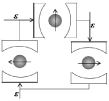
Figure 1: Schematic setup of the supposed system. Three two-level atoms are trapped in separate optical cavities linked via optical fibers. Each of the cavities is driven by an external field. Every atom is coupled to a local laser field.

Using the input-output theory, taking the adiabatic approximation ^[20] and applying the methods developed in Refs. [2], we obtain the effective Hamiltonian of the global system as $H_{eff}=H_{zz}$, where $H_{zz}=J(\sigma_{1}^{z}\sigma_{2}^{z}+\sigma_{2}^{z}\sigma_{3}^{z}+\sigma_{3}^{z}\sigma_{1}^{z})$, $\sigma_{i}^{z}$ is spin operators of atom i. And $J=2\kappa\chi^{2}Im\left\{|\alpha|^{2}(Me^{i\phi}+\kappa e^{i2\phi})/(M^{3}-W^{3})\right\}$, where $\kappa$ is the cavity leaking rate, $\chi=\frac{g^{2}}{\Delta}$, $g$ is the coupling strength between atom and cavity field, $\Delta$ is the detuning. In deducing $H_{eff}$, the condition $\Delta\approx\kappa\gg g$ is assumed, $M=i\Delta+\kappa$, $W^{3}=\kappa^{3}e^{i3\phi}$. $\phi_{21}$, $\phi$ is the phase delay caused by the photon transmission along optical fiber. And $\alpha=\varepsilon\frac{M^{2}+M\kappa e^{i\phi}+\kappa^{2}e^{i2\phi}}{M^{3}-W^{3}}$. Such a system is undoubtedly an Ising ring model with uniform coupling strengthes.

It has been approved that, in an isotropic Heisenberg model, the arbitrarily perfect QST can be achieved only by applying a magnetic field along the spin chain ^[13]. Thus, we assume local weak laser fields are applied to resonantly interact with the atoms. Without losing of generality, we allow a simple spatial variation of the laser fields so that the Rabi frequencies are different for individual atoms. The effective Hamiltonian is now written as $H_{eff}=H_{zz}+H_{x}$, where $H_{x}=\sum\limits_{i}\Gamma_{i}\sigma_{x},\sigma_{x}=(\sigma_{i}^{-}+\sigma_{i}^{+})$, $\sigma_{i}^{+}(\sigma_{i}^{-})$ is raising (lowering) operator of atom $i$. This can be interpreted as an Ising ring with electromagnetic fields applied on individual spins in perpendicular direction. The system plays an important role in quantum information process since two-atom entangled stated can be generated in such system by synchronously turning off the local laser fields ^[21-23]. This paper aims to study the QST governed by the Hamiltonian. Under the condition $\Gamma_{i}\ll J$, the secular part of the effective Hamiltonian can be obtained through the transformation $UH_{x}U^{-1}$, $U=e^{-iH_{zz}t}$, as ^[24]

$$\tilde{H}=\sum\limits_{ijk}\frac{\Gamma_{i}}{2}\sigma_{i}^{x}(1-\sigma_{j}^{z}\sigma_{k}^{z}).$$ (1)

where the subscripts $ijk$ are permutations of $1,2,3$. The straight forward interpretation of this Hamiltonian is: the spin of an atom in the Ising ring flips if and only if its two neighbors have opposite spins.

The task of arbitrary unknown quantum state transfer (QST) between two two-level systems a and b is to accomplish the implementation $(\alpha|e\rangle_{a}+\beta|g\rangle_{a})\otimes|g\rangle_{b}\longrightarrow|g\rangle_{a}\otimes(\alpha|e\rangle_{b}+\beta|g\rangle_{b})$ deterministically, where $\alpha$ and $\beta$ are unknown complex number and meet the condition of normalization, and the former in above equation is the inputting initial state while the latter is the outputting target state.

To this end, we assume atom 1 is inputting qubit and initially in coherent state $\alpha|e\rangle_{1}+\beta|g\rangle_{1}$, atom 2 is outputting qubit and initially in ground state, atom 3 is an auxiliary qubit and initially in ground state, and suppose the local laser field applied on atom 3 is kept zero, which leads to an unchanged state of atom 3. The secular part of the effective Hamiltonian can be written as $\tilde{H}=\Gamma_{1}\sigma_{1}^{x}(1-\frac{1}{2}\sigma_{2}^{z}\sigma_{3}^{z})+\Gamma_{2}\sigma_{2}^{x}(1-\frac{1}{2}\sigma_{1}^{z}\sigma_{3}^{z})$. The evolution of the first term of initial state $(\alpha|e\rangle_{1}+\beta|g\rangle_{1})\otimes|g\rangle_{2}\otimes|g\rangle_{3}$ is restricted within the subspace spanned by the following basis vectors

$$|\phi_{1}\rangle=|e\rangle_{1}|e\rangle_{2}|g\rangle_{3},|\phi_{2}\rangle=|e\rangle_{1}|g\rangle_{2}|g\rangle_{3},|\phi_{3}\rangle=|g\rangle_{1}|e\rangle_{2}|g\rangle_{3},$$ (2)

while the second term remains unchanged. The Hamiltonian in Eq. (7) is now written as

$$\tilde{H}=\left(\begin{array}[]{ccc}0&\Gamma_{2}&\Gamma_{1}\\ \Gamma_{2}&0&0\\ \Gamma_{1}&0&0\\ \end{array}\right).$$ (6)

The eigenvalues of the Hamiltonian can be obtained as $E_{12}=\pm\sqrt{\Gamma_{1}^{2}+\Gamma_{2}^{2}}$,$E_{3}=0$, and the corresponding eigenvectors are

$$|\psi\rangle_{i}=\sum\limits_{j}S_{ij}|\phi_{j}\rangle$$ (7)

where

$$S=\left(\begin{array}[]{ccc}\frac{1}{\sqrt{2}}&\frac{\Gamma_{2}}{\sqrt{2(\Gamma_{1}^{2}+\Gamma_{2}^{2})}}&\frac{\Gamma_{1}}{\sqrt{2(\Gamma_{1}^{2}+\Gamma_{2}^{2})}}\\ -\frac{1}{\sqrt{2}}&\frac{\Gamma_{2}}{\sqrt{2(B_{1}^{2}+\Gamma_{2}^{2})}}&\frac{\Gamma_{1}}{\sqrt{2(\Gamma_{1}^{2}+\Gamma_{2}^{2})}}\\ 0&-\frac{\Gamma_{1}}{\sqrt{\Gamma_{1}^{2}+\Gamma_{2}^{2}}}&\frac{\Gamma_{2}}{\sqrt{\Gamma_{1}^{2}+\Gamma_{2}^{2}}}\\ \end{array}\right)$$ (11)

, which represents unitary transformation matrix between eigenvectors and basis vectors. For initial system state $|\Psi(0)\rangle=\sum\limits_{i}c_{i}(0)|\phi_{i}\rangle$, the evolving global system state can be written as $|\Psi(t)\rangle=\sum\limits_{i}c_{i}(t)|\phi_{i}\rangle$ and is governed by the Schrödinger equation $i\frac{\partial|\Psi(t)\rangle}{\partial t}=\tilde{H}|\Psi(t)\rangle$. The coefficients $c_{i}(t)$ are then given by ^[9] $c_{i}(t)=\sum\limits_{j}[S^{-1}]_{ij}[Sc(0)]_{j}e^{-iE_{j}t}$, where $c(0)=[c_{1}(0),c_{2}(0),c_{3}(0)]^{T}$.

For initial coefficients $c(0)=[0,\alpha,0]^{T}$, the coefficients can be obtained as

$$c_{1}(t) = -i\frac{\alpha\Gamma_{2}}{\Omega}\textrm{sin}\Omega t,$$

$$c_{2}(t) = \frac{\alpha\Gamma_{1}^{2}}{\Omega^{2}}+\frac{\alpha\Gamma_{2}^{2}}{\Omega^{2}}\textrm{cos}\Omega t$$

$$c_{3}(t) = \frac{-\alpha\Gamma_{1}\Gamma_{2}}{\Omega^{2}}+\frac{\alpha\Gamma_{1}\Gamma_{2}}{\Omega^{2}}\textrm{cos}\Omega t.$$ (12)

where $\Omega=\sqrt{\Gamma_{1}^{2}+\Gamma_{2}^{2}}$.

It is easily shown that, one can take $\Gamma_{1}=\Gamma_{2}=\Gamma_{0}$ and turn off the local laser fields applied to atom 1 and atom 2 synchronously at $t_{p}=\frac{(2k-1)\pi}{\Omega},k=1,2,3,...$ and obtain the system state as

$$|\Psi(t_{p_{0}})\rangle=|g\rangle_{1}\otimes(-\alpha|e\rangle_{2}+\beta|g\rangle_{2})|g\rangle_{3}.$$ (13)

The above state differs from the target state $|g\rangle_{1}\otimes(\alpha|e\rangle_{2}+\beta|g\rangle_{2})\otimes|g\rangle_{3}$ due to a minus sign. To obtain the target state exactly, one may program the operating process as in Table. 1 (the term '$\pi$ pulse' in the table is used to denote an equivalent evaluating time $t_{p_{0}}=\frac{\pi}{\Omega}$):

Table. 1 Operation sequence for implementing QST
operation sequence	system state
$\Gamma_{1}=\Gamma_{3}=\Gamma_{0},\Gamma_{2}=0$	initial state $(\alpha|e\rangle_{1}+\beta|g\rangle_{1})|g\rangle_{2}|g\rangle_{3}$
$\pi$ pulse on atoms 1 and 3	$|g\rangle_{1}|g\rangle_{2}(-\alpha|e\rangle_{3}+\beta|g\rangle_{3})$
$\Gamma_{2}=\Gamma_{3}=\Gamma_{0},\Gamma_{2}=0$	$|g\rangle_{1}|g\rangle_{2}(-\alpha|e\rangle_{3}+\beta|g\rangle_{3})$
$\pi$ pulse on atoms 2 and 3	target state $|g\rangle_{1}(\alpha|e\rangle_{2}+\beta|g\rangle_{2})|g\rangle_{3}$

The above operating process can be interpreted as two steps:

Firstly, turning on the laser field acting on atom 1 and 3 while keeping the laser field acting atom 3 zero. At the specific time $t_{p_{1}}=\frac{(2k-1)\pi}{\Omega},k=1,2,3,...$, turning off the laser fields synchronously.

Secondly, turning on the laser field acting on atom 2 and 3 while keeping the laser field acting atom 1 zero. At the specific time $t_{p_{2}}=\frac{(2k-1)\pi}{\Omega},k=1,2,3,...$, turning off the laser fields synchronously.

In this procedure, one do not need to know the values of coefficients $\alpha$ and $\beta$, and do not require any methods of quantum coincidence measurement on atoms. An unknown QST is implemented deterministically with $100\%$ success probability.

To illustrate the the efficiency of the QST, not only at specific times, but also in overall view of time scales, we plot the fidelity of QST between atoms 1 and 2 with respect to operating times $t_{1}$, which represents the operating time of the first step, and $t_{2}$, which denotes that of the second step. The average fidelity is defined as ^[9]

$$F=\frac{1}{2\pi}\int_{0}^{2\pi}|\langle\Psi_{f}|\Psi(t)\rangle|^{2}d\theta$$ (14)

where, $|\Psi_{f}\rangle$ is the target state. In Fig. 2 (a), it can be seen that the overall quantity of fidelity is governed by operating times $t_{p_{1}}$ and $t_{p_{2}}$ almost equally. The fidelity periodically reaches the maximum 1 at specific times $t_{p_{1}}=t_{p_{2}}=\frac{\pi}{\Omega}$. The time cost of the scheme can be estimated as $t_{p}\approx\frac{2\pi}{\Omega}$.

The above results explicitly demonstrate a deterministic two-step QST scheme between atoms 1 and 2 which is accomplished by only turning on two identical local laser fields applied on atoms 1 and 3 and turning them off at typical times synchronously, and duplicate the step for atoms 2 and 3. Similarly, QST between atoms 2 and 3 or between atoms 1 and 3 can be accomplished similarly.

So, the total procedure of the scheme implementation consists only two steps: a step turning on/off the laser fields synchronously for inputting atom and auxiliary atom and repeat the step for auxiliary atom and outputting atom.

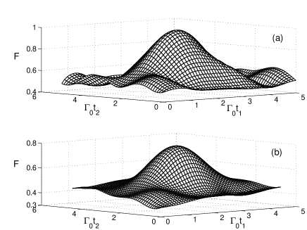
Figure 2: Fidelity of QST between atoms 1 and 2 with respect to operating times $t_{1}$ and $t_{2}$ for (a) atomic spontaneous emission rate $\gamma=0$, (b) atomic spontaneous emission rate $\gamma=0.1\Gamma_{0}$

In this model, the leakage of cavity fields is assumed to be large enough to keep the validity of the adiabatic approximation for obtaining effective Hamiltonian. While, the inevitable atomic spontaneous emission still challenges the efficiency of the scheme and results in a dissipative effect, which can be estimated by adding a non-Hermitian conditional term to the Hamiltonian in Eqn. (1)^[25]. The global Hamiltonian can be written as $H_{s}=-i\gamma\sum\limits_{i}|e\rangle_{i}\langle e|+\tilde{H}$, where $\gamma$ represents the atomic spontaneous emission rate. In the subspace spanned by $|\phi_{1}\rangle=|e\rangle_{1}|g\rangle_{2}|e\rangle_{3}$, $|\phi_{2}\rangle=|e\rangle_{1}|g\rangle_{2}|g\rangle_{3}$, $|\phi_{3}\rangle=|g\rangle_{1}|g\rangle_{2}|e\rangle_{3}$, for initial state $|e\rangle_{1}|g\rangle_{2}|g\rangle_{3}$, the evolved coefficients can be obtained as

$$c_{1}(t) = -\frac{i\alpha\Gamma_{3}}{\Lambda}e^{-\frac{3}{2}\gamma t}\textrm{sin}\Lambda t,$$

$$c_{2}(t) = \frac{\alpha\Gamma_{1}^{2}}{\Omega^{2}}e^{-\gamma t}(1+\frac{\Gamma_{3}^{2}}{\Gamma_{1}^{2}}e^{-\frac{\gamma t}{2}}\textrm{cos}\Lambda t+\frac{\gamma}{\Lambda}\frac{\Gamma_{3}^{2}}{\Gamma_{1}^{2}}e^{-\frac{\gamma t}{2}}\textrm{sin}\Lambda t),$$

$$c_{3}(t) = \frac{\alpha\Gamma_{1}\Gamma_{3}}{\Omega^{2}}e^{-\gamma t}(-1+e^{-\frac{\gamma t}{2}}\textrm{cos}\Lambda t+\frac{\gamma}{\Lambda}e^{-\frac{\gamma t}{2}}\textrm{sin}\Lambda t),$$ (15)

where $\Lambda=\sqrt{\Gamma_{1}^{2}+\Gamma_{3}^{2}-\frac{\gamma^{2}}{4}}$.

Taking $\Gamma_{1}=\Gamma_{3}=\Gamma_{0}$ and shutting down the laser fields applied to atom 1 and atom 3 synchronously at specific time $t_{p_{1}}=\frac{(2k-1)\pi}{\Lambda},k=1,2,3,...$ , one can obtain the system state as

$$\Psi(t_{p_{1}}) = \alpha A_{1}e^{-\gamma t_{p_{1}}}|e\rangle_{1}|g\rangle_{2}|g\rangle_{3}$$ (16)

$$- \alpha B_{1}e^{-\gamma t_{p_{1}}}|g\rangle_{1}|g\rangle_{2}|e\rangle_{3}+\eta\beta|g\rangle_{1}|g\rangle_{2}|g\rangle_{3},$$

where $\eta$ is an additional normalized factor, $A_{1}=\frac{(1-e^{-\frac{\gamma t_{p_{1}}}{2}})}{2},B_{1}=\frac{(1+e^{-\frac{\gamma t_{p_{1}}}{2}})}{2}$. Now, we let the above state be new inputting initial state without delay and take $\Gamma_{2}=\Gamma_{3}=\Gamma_{0}$, and shutting down the laser fields applied to atom 2 and atom 3 synchronously at specific time $t_{p_{2}}=\frac{(2k-1)\pi}{\Lambda},k=1,2,3,...$. It can be proved that, under this condition, there is no transition between the first term in Eqn. (10) and other three-atom excited states such as $|e\rangle_{1}|e\rangle_{2}|g\rangle_{3}$, $|e\rangle_{1}|g\rangle_{2}|e\rangle_{3}$. After some complicated calculation, the system state can be obtained analytically as

$$|\Psi(t_{p}) = \alpha e^{-\gamma(t_{p_{1}}+t_{p_{2}})}B_{1}B_{2}|g\rangle_{1}|e\rangle_{2}|g\rangle_{3}$$

$$- \alpha e^{-\gamma(t_{p_{1}}+t_{p_{2}})}B_{1}A_{2}|g\rangle_{1}|g\rangle_{2}|e\rangle_{3}$$

$$- \alpha e^{-\gamma(t_{p_{1}}+3t_{p_{2}})}A_{1}|e\rangle_{1}|g\rangle_{2}|g\rangle_{3}+\lambda\beta|g\rangle_{1}|g\rangle_{2}|g\rangle_{3},$$

where $A_{2}=\frac{(1-e^{-\frac{\gamma t_{p_{2}}}{2}})}{2},B_{2}=\frac{(1+e^{-\frac{\gamma t_{p_{2}}}{2}})}{2}$, $\lambda$ is an additional normalized factor. The time cost of the scheme is now estimated as $t_{p}=t_{p_{1}}+t_{p_{2}}\approx\frac{2\pi}{\Lambda}$.

Figure 3: Fidelity of QST between atoms 1 and 2 with respect to (a) atomic spontaneous emission, the operating time $t_{p_{1}}=t_{p_{2}}=\frac{\pi}{\Lambda}$, and (b) operating time error $(t-t_{p})\Lambda/\pi$, where the triangle indicates the maximum value of fidelity, $\gamma=0$ for solid line, $\gamma=0.05\Gamma_{0}$ for dashed line, $\gamma=0.1\Gamma_{0}$ for dotted line.

In Fig. 2 (b), we plot the fidelity of QST with respect to operating time $t_{p_{1}}$ and $t_{p_{2}}$ for atomic spontaneous emission rate $\gamma=0.1\Gamma_{0}$. Obviously, the atomic spontaneous emission reduces the overall quantity of fidelity and smoothing the oscillation of the fidelity. In Fig. 3 (a), we plot fidelity of QST between atoms 1 and 2 with respect to atomic spontaneous emission. Obviously, the spontaneous emission monotonically decreases the maximum quantity of fidelity of QST, which corresponds to the strict operating time condition $t_{p_{1}}=t_{p_{2}}=\frac{\pi}{\Lambda}$. While, in practical case, operating time error emerges inevitably. The existence of operating time error can lead to a more complicated system state includes $|e\rangle_{1}|e\rangle_{2}|g\rangle_{3}$, $|e\rangle_{1}|g\rangle_{2}|e\rangle_{3}$, $|g\rangle_{1}|e\rangle_{2}|e\rangle_{3}$, $|e\rangle_{1}|g\rangle_{2}|g\rangle_{3}$, $|g\rangle_{1}|g\rangle_{2}|e\rangle_{3}$, $|g\rangle_{1}|e\rangle_{2}|g\rangle_{3}$. Only the last term contributes to the fidelity of QST. In Fig. 3 (b), we plot fidelity of QST between atoms 1 and 2 with respect to operating time error $(t-t_{p})\Lambda/\pi$ for different atomic spontaneous emission rates. It is interesting that operating time error, for larger spontaneous emission, on one hand decreases the maximum quantity of fidelity, on the other hand reduces the time cost for achieving maximum quantity of fidelity and, in other words, speeds up the implementation of QST, which is the cooperative influence of spontaneous emission and operating time error. Further more, the sensitivity of fidelity to operating time error is decreased for larger spontaneous emission.

In summary, we have discussed an arbitrary QST scheme in a system contains three distant atoms by simply replicating the operation of synchronously turning on/off the locally applied laser fields for individual atoms. The auxiliary atom is used to avoid additional single qubit phase shift operation and the resulting QST is deterministic and in 100% fidelity. We discuss the affect of atomic spontaneous emission on QST. It is shown that the atomic spontaneous emission decreases the quantity of fidelity, while the cooperative influence of spontaneous emission and operating time error reduces the time cost $\frac{2\pi}{\Lambda}$ for maximum fidelity and thus speeds up the implementation of QST. It has been demonstrated that the dissipation of the photon leakage along optical fibers can be included in the spin-spin coupling coefficients by replacing the phase factor $e^{i\phi}$ in Eq. (3) with $e^{i\phi-\nu L}$ ^[2] , where $\nu$ is the fiber decay per meter and $L$ is the length of the fiber between atoms $i$ and $j$. For typical fibers ^[26], the decay per meter is $\nu\thickapprox 0.08$. The spin-spin coupling coefficient $J_{0}^{{}^{\prime}}$ is now about $90\%$ of $J_{0}$. The rotating wave approximation in deriving secular part of effective Hamiltonian is still kept valid under the condition $\Gamma_{i}\ll J_{0}^{{}^{\prime}}\thickapprox 0.9J_{0}$. So the QST gate still works with high fidelity. Furthermore, we have assumed $\kappa\gg g$ in the calculation of deriving effective Ising model, which ensures the scheme is insensitive to the slight variation of strong leakage rate. As is concluded, the scheme works in a robust way since both the affected aspects of fiber lossy and cavity dissipation can be neglected. It should also be noticed that to avoid the inevitable time-delay affect caused by mismatch of practical and theoretical controlling times ^[27], remedial methods such as Lyapunov control can be used in the extended scheme. Many of the present schemes only contain two atoms trapped in separated cavities. From a realistic point of view, a robust quantum network must contains many distant quantum nodes. QST must be implemented between any two quantum nodes in high fidelity. The model used and the results obtained in this scheme may act as a possible candidate.

We thank Professor Dian Min Tong and Professor Dong Mi for helpful discussions and their encouragement. This work is supported by NSF of China under Grant No. 11305021 and the Fundamental Research Funds for the Central Universities.

References

- (1) Serafini A, Mancini S and Bose S 2006 Phys. Rev. Lett. 96 010503
- (2) Mancini S and Bose S 2004 Phys. Rev. A 70 022307
- (3) Zhan X, Qin H, Bian Z H, Li J and Xue P 2014 Phys. Rev. A 90012331
- (4) Rosenfeld W, Berner S, Volz J, Weber M and Weinfurter H 2007 Phys. Rev. Lett. 98 050504
- (5) Cho J and Lee H W 2005 Phys. Rev. Lett. 95 160501
- (6) Razavi M and Shapiro J H 2006 Phys. Rev. A 73 042303
- (7) Zheng S B and Guo G C 2006 Phys. Rev. A 73 032329
- (8) Duan L M, Madsen M J, Moehring D L, Maunz P, Kohn R N and Monroe C 2006 Phys. Rev. A 73 062324
- (9) Yin Z Q and Li F L 2007 Phys. Rev. A 75 012324
- (10) Lu D M and Zheng S B 2007 Chin. Phys. Lett. 24 596
- (11) Wang Y D and Clerk A A 2012 Phys. Rev. Lett. 108 153603
- (12) Franco C Di, Paternostro M and Kim M S 2008 Phys. Rev. Lett. 101 230502
- (13) Korzekwa K, Machnikowski P and Horodecki P 2014 Phys. Rev. A 89 062301
- (14) Liu Y and Zhou D L 2014 Phys. Rev. A 89 062331
- (15) Biswas A and Agarwal G S 2004 Phys. Rev. A 70 022323
- (16) Bevilacqua G and Renzoni F 2013 Phys. Rev. A 88 033817
- (17) Moehring D L, Maunz P, Olmschenk S, Younge K C, Matsukevich D N, Duan L M and Monroe C 2007 Nature 449 68
- (18) Zhong Z R, Zhang B, Lin X and Su W J 2011 Chin. Phys. lett. 28 120303
- (19) Guo Y Q, Chen J and Song H S 2006 Chin. Phys. Lett. 23 1088
- (20) Walls D F and Milburn G J 1994 Quantum Optics (Berlin: Springer)chap 7 p121
- (21) Štemlmachovič P and Bužek V 2004 Phys. Rev. A 70 032313
- (22) Furman G B, Meerovich V M and Sokolovsky V L 2008 Phys. Rev. A 77 062330
- (23) Guo Y Q, Zhong H Y, Zhang Y H and Song H S 2008 Chin. Phys. Lett. 25 2362
- (24) Lee J S and Khitrin A K 2005 Phys. Rev. A 71 062338
- (25) Cho J and Lee H W 2005 Phys. Rev. Lett. 95 160501
- (26) Tittel W, Brendel J, Gisin B, Herzog T, Zbinden H and Gisin N 1998 Phys. Rve. A 57 3229
- (27) Yi X X, Wu S L, Wu C F, Feng X L and Oh C H 2011 J. Phys. B: At. Mol. Opt. Phys. 44 195503