Contract-Based Interference Coordination in Heterogeneous Cloud Radio Access Networks

Abstract

Heterogeneous cloud radio access networks (H-CRANs) are potential solutions to improve both spectral and energy efficiencies by embedding cloud computing into heterogeneous networks (HetNets). The interference among remote radio heads (RRHs) can be suppressed with centralized cooperative processing in the base band unit (BBU) pool, while the inter-tier interference between RRHs and macro base stations (MBSs) is still challenging in H-CRANs. In this paper, to mitigate this inter-tier interference, a contract-based interference coordination framework is proposed, where three scheduling schemes are involved, and the downlink transmission interval is divided into three phases accordingly. The core idea of the proposed framework is that the BBU pool covering all RRHs is selected as the principal that would offer a contract to the MBS, and the MBS as the agent decides whether to accept the contract or not according to an individual rational constraint. An optimal contract design that maximizes the rate-based utility is derived when perfect channel state information (CSI) is acquired at both principal and agent. Furthermore, contract optimization under the situation where only the partial CSI can be obtained from practical channel estimation is addressed as well. Monte Carlo simulations are provided to confirm the analysis, and simulation results show that the proposed framework can significantly increase the transmission data rates over baselines, thus demonstrating the effectiveness of the proposed contract-based solution.

I Introduction

The demand for high-speed and high-quality data applications is expected to increase explosively in the next generation cellular network, also called the fifth generation (5G), along with the rapid growth of capital expenditure and energy consumption [1]. Since the traditional third generation (3G) and fourth generation (4G) cellular networks, originally devised for enlarging the coverage areas and optimized for the homogenous traffic, are reaching their limits, heterogeneous networks (HetNets) have attracted intense interest from both academia and industry [2]. HetNets offer the advantages of serving dense customer populations in hot spots with low power nodes (LPNs) (e.g., pico base stations, femto base stations, small cell base stations, etc.), while providing ubiquitous coverage with macro base stations (MBSs), and reducing the energy consumption [3]. Unfortunately, high densities of LPNs incur severe interference, which restricts performance gains and commercial applications of HetNets [4]. To suppress inter-LPN and inter-tier interference, coordinated multi-point (CoMP) transmission and reception has been presented as one of the most promising techniques in 4G systems [5]. Though performance gains of CoMP are significant under ideal assumptions, they degrade with increasing density of LPNs due to the non-ideal information exchange and cooperation among LPNs. On the one hand, it has been demonstrated that the performance of the downlink CoMP with zero-forcing beamforming (ZFBF) depends heavily on time delay, and thus the ZFBF design should be fairly conservative [6]. Further, it has been shown that CoMP ZFBF has no throughput gain when the overhead channel delay is larger than 60% of the channel coherence time. On the other hand, it has been reported in [7] that the average spectral efficiency (SE) gain of uplink CoMP in downtown Dresden field trials is only about 20% with non-ideal backhaul and distributed cooperation processing located on MBSs. Hence, novel system architectures and advanced signal processing techniques are needed to fully realize the potential gains of HetNets.

Meanwhile, cloud computing technology has emerged as a promising solution for providing good performance in terms of both SE and energy efficiency (EE) across software defined wireless communication networks [8]. By leveraging cloud computing technologies, the storage and computation originally provided in the physical layer can be migrated into the “cloud” to avoid redundant resource consumption and to achieve the overall optimization of resource allocation via centralized processing [9]. As an application of cloud computing to radio access networks, the cloud radio access network (C-RAN) has been proposed to achieve large-scale cooperative processing gains, though the constrained fronthaul link between the remote radio head (RRH) and the baseband unit (BBU) pool presents a performance bottleneck [10]. Since the C-RAN is mainly utilized to provide high data rates in hot spots, real-time voice service and control signalling are not efficiently supported. In order to avoid the significant signalling overhead through decoupling the user plane and control plane in RRHs, the traditional C-RAN must be enhanced and even evolved.

Motivated by the aforementioned challenges of both HetNets and C-RANs, an advanced solution known as the heterogeneous cloud radio access network (H-CRAN) is introduced in [11]. The motivation of H-CRANs is to avoid inter-LPN interference existing in HetNets through connecting to a “signal processing cloud” with high-speed optical fibers[12]. As such, the baseband datapath processing as well as the radio resource control for LPNs are moved to the BBU pool so as to take advantage of cloud computing capabilities, which can fully exploit the cooperation processing gains, lower operating expenses, improve SE performance, and decrease energy consumption of the wireless infrastructure. The simplified LPNs are converted into RRHs, i.e., only the front radio frequency (RF) and simple symbol processing functionalities are configured in RRHs, while the other important baseband physical processing and procedures of the upper layers are jointly executed in the BBU pool.

In H-CRANs, the control and user planes are decoupled, and the delivery of control and broadcast signalling is shifted from RRHs to MBSs, which alleviates the capacity and time delay constraints on the fronthaul. Therefore, RRHs are mainly used to provide high bit rates with high EE performances, while the MBS is deployed to guarantee seamless coverage and deliver the overall control signalling. With the help of MBSs, unnecessary handover and re-association can be avoided. The adaptive signaling/control mechanism between connection-oriented and connectionless modes is supported in H-CRANs, which can achieve significant overhead savings in the radio connection/release by moving away from a pure connection-oriented mechanism.

As shown in Fig. 1, the BBU pool is interfaced to MBSs for coordinating the cross-tier interference between RRHs and MBSs. The data and control interfaces between the BBU pool and the MBS are S1 and X2, respectively, which are inherited from definitions of the $3^{rd}$ generation partnership project (3GPP) standards. With the help of centralized large-scale cooperative processing in the BBU pool, the intra-tier interference can be fully suppressed, while the inter-tier interference between RRHs and MBSs still present challenges to improving SE and EE performance. Significant attention has been paid to inter-tier interference collaboration [13, 14] and radio resource cooperative management techniques [15] to alleviate inter-tier interference. As these works are focused primarily on HetNets, new models and methods are needed for H-CRANs.

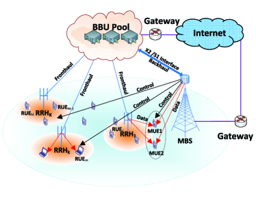
Figure 1: System model of the H-CRAN with one MBS and $K$ RRHs.

Intuitively, game theory is a useful tool for examining the inter-tier interference problem, and the published literature for HetNets has presented using this approach. For example, a Stackelberg game model has been used in [17] to design a distributed radio resource algorithm, and its adaption to hierarchical problems such as hierarchical power control has been considered in [18]. More specifically, a Stackelberg game with a single leader and multiple followers is formulated to study joint objective optimization of the macrocell and femtocells subject to a maximum interference power constraint at the MBS in [19]. In [20], a hierarchical game framework with multiple leaders and multiple followers is adopted to investigate uplink power allocation to mitigate inter-tier interference in two-tier femtocell networks. In order, for the Stackelberg game, to reach an equilibrium, players involved in the game have to interact periodically, which leads to high latency and signalling overhead. Furthermore, the incentive in the Stackelberg game model is ineffective if the information is asymmetric between the leader and follower. To overcome these issues, an advanced game model with proper incentive mechanisms and regarding the limited overhead is preferred.

To overcome the aforementioned problems in the Stackelberg model, contract-based game theory has recently been applied to aspects of spectrum sharing and relay selection. In [21], to solve the cooperative spectrum sharing problem under incomplete channel state information (CSI) in cognitive radio networks, a resource-exchange scheme is proposed and the corresponding optimal contract model is designed. The problem of spectrum trading with a single primary user selling its idle spectrum to multiple secondary users is investigated in [22], where a money-exchange based contract is offered by the primary user containing a set of different items each intended for a specific consumer type. In [23], under an asymmetric information scenario where the source is not well informed about the CSI of potential relays, a contract based game theory model is designed to help the source select relays for optimizing the throughput. Motivated by these existing works, since the cooperative processing capabilities and acquired CSI are significantly different between the BBU pool and the MBS in H-CRANs, contract-based game theory is a promising technique for modeling the inter-tier interference coordination mechanism under information asymmetry.

Note that ideal inter-tier interference coordination depends critically on having accurate CSI for all transmitters and receivers [24]; however, this assumption is non-trivial especially in view of the overwhelming signalling overhead and the inevitable existence of CSI distortion in practical systems [25]. In previous studies, CSI errors are typically modeled as zero-mean complex Gaussian random variables without taking the practical training process and channel estimation methods into account [26]. In order to present a realistic scenario, not only the impact of imperfect CSI but also the corresponding training based channel estimation technique should be considered when examining contract-based interference coordination in H-CRANs.

In this paper, we propose a contract-based interference coordination framework to mitigate the inter-tier interference between RRHs and MBSs in H-CRANs. Based on the proposed framework, different scheduling schemes can be utilized jointly to achieve performance gains. Specifically, three scheduling schemes are embedded into the proposed framework in this paper, and the downlink transmission is divided into three phases accordingly. At the first phase, RRHs help MBSs serve macro-cell user equipments (MUEs), which is termed the RRH-alone with UEs-all scheme. At the second phase, MBSs let RRHs use all radio resources to serve the associated UEs (denoted by RUEs), which is called the RRH-alone with RUEs-only scheme. Then at the third phase, RRHs and MBSs serve their own UEs separately, namely the RRH-MBS with UEs-separated scheme. Note that these three schemes are examples merely used to show the principles of the proposed contract-based inter-tier interference coordination framework, and other inter-tier interference coordination schemes can be embedded into this framework, or replace these three schemes. Through the contract-based interference coordination framework, RRHs and MBSs establish a mutually beneficial relationship, which can be effectively modeled and optimized by using contract-based game theory. The main contributions of this paper are summarized as follows:

• To coordinate the inter-LPN interference in HetNets, and to compensate for the substantial fronthaul overhead and processing in conventional C-RAN, the H-CRAN is considered in this paper, which incorporates advantages of both the HetNet and C-RAN. The H-CRAN decouples the control and user planes, and thus RRHs are mainly used to provide high data rates via cloud computing to suppress the intra-tier interference, while the MBS is deployed to guarantee seamless coverage and deliver all control and broadcast signals.

• Since the cooperative processing capability and acquired CSI between the BBU pool and MBS are asymmetric, a contract-based interference coordination framework is proposed to coordinate the inter-tier interference between RRHs and MBSs, where the BBU pool and the MBS are modeled as the principal and agent, respectively. Based on the proposed coordination framework, three scheduling schemes, namely RRH-alone with UEs-all, RRH-alone with RUEs-only, and RRH-MBS with UEs-separated, are adaptively utilized. Accordingly, the downlink transmission in each interval is divided into three phases.

• With complete CSI, i.e., the BBU pool can acquire the perfect global CSI, sufficient and necessary conditions for a feasible contract are presented. An contract design that maximizes a rate-based utility is derived to achieve the optimized transmission duration for these three phases and to obtain the optimized received power allocation for RUEs and MUEs. Theoretical analysis indicates that the optimal rate-based utility is achieved when the time duration of the third phase is zero, i.e., the RRH-MBS with UEs-separated scheme is not triggered due to the large inter-tier interference even though the fairness power control algorithm is applied.

• Considering the imperfect CSI acquired in piratical H-CRANs, training and channel estimation schemes are presented to obtain partial CSI. Based on the estimated partial CSI, contract design and optimization for the presented framework are addressed. Specifically, sufficient and necessary conditions for a feasible contract under partial CSI are presented, which are individually rational and incentive compatible. In addition, the optimization problem to determine the contract that maximizes the rate-based utility is formulated. Moreover, an optimal contract design is derived when the number of RRHs is large.

The rest of this paper is organized as follows: Section II describes the system model and the proposed interference coordination framework. In Section III, an optimal contract design with ideal and complete CSI is presented. Then in Section IV, contract design with practical channel estimation is considered. Numerical results are shown in Section V, followed by conclusions in Section VI.

Notation: The transpose, inverse, and Hermitian of matrices are denoted by $\left(\cdot\right)^{T}$, $\left(\cdot\right)^{-1}$, and $\left(\cdot\right)^{H}$, respectively. $\|\cdot\|$ denotes the two-norm of vectors. $\mathbf{diag}\left(e_{1},e_{2},\ldots,e_{N}\right)$ is the $N\times N$ diagonal matrix. $\mathbf{I}_{K}$ represents the $K\times K$ dimensional unitary diagonal matrix. $\mathcal{E}\{\cdot\}$ denotes the expectation of random variables and $\dot{\left(\cdot\right)}$ denotes the first order derivative. For convenience, the abbreviations are listed in Table I.

TABLE I: Summary of Abbreviations

AWGN	additive white Gaussian noise
BBU	base band unit
cdf	cumulative density function
CICF	contract-based interference coordination framework
CoMP	coordinated multi-point
C-RAN	cloud radio access network
CSI	channel state information
EE	energy efficiency
FRPC	frequency reuse with power control
H-CRAN	heterogeneous cloud radio access network
HetNet	heterogeneous network
IC	incentive compatible
IR	individual rational
KKT	Karush-Kuhn-Tucker
LPN	low power node
LSE	least-squares estimate
MBS	macro base station
MSE	mean-square error
MUE	macro-cell user equipment
OFDMA	orthogonal frequency division multiple access
pdf	probability density function
RB	resource block
RF	radio frequency
RRH	remote radio head
RUE	remote radio head served user equipment
SE	spectral efficiency
SNR	signal-to-noise ratio
TDD	time division duplex
TDIC	time domain interference cancelation
TTI	time transmission interval
UE	user equipment
ZFBF	zero-forcing beamforming

II System Model and Interference Coordinated Framework

The discussed H-CRAN consists of one BBU pool, $K$ RRHs and one MBS, in which each RRH connects with the BBU pool through an ideal optical fiber, and the MBS connects with the BBU pool ideally with no constraints. It is assumed that all $K$ RRHs cooperate, and they share the same radio resources with the MBS. The radio resources are allocated to different MUEs using orthogonal frequency division multiple access (OFDMA). It is assumed that each node has a single antenna, and thus for each resource block (RB) in the OFDMA based H-CRAN, only one MUE will be served by the MBS, and at most $K$ RUEs will be associated with the $K$ RRHs. Without loss of generality, $M$ ($M<K$) RUEs and one MUE can share the same RB in OFDMA based H-CRAN systems. When $M\!\geq\!K$, $K$ RUEs are selected to be auto-scheduled [27]. We note that a number of synchronization solutions for distributed antenna and virtual MIMO systems, e.g., the protocol in [29] and post-facto synchronization [30], can be effectively applied to accomplish the synchronization among RRHs. Thus we assume that all RRHs and the MBS can be perfectly synchronized.

Downlink transmission is considered, in which the BBU pool sends individual data flows to RUEs via RRHs, and the MBS transmits the data flows to MUEs. The radio channel matrix between RRHs and RUEs is denoted by $\mathbf{G}$ whose $\left(m,k\right)$-th entry $g_{mk}$ represents the channel coefficient between the $k$-th RRH and the $m$-th RUE. The channel coefficient between the MBS and MUE is denoted by $g_{B}$. Let $f_{kM}$ denote the radio channel coefficient between the $k$-th RRH and MUE, and $f_{Bm}$ represent the channel coefficient between the $m$-th RUE and MBS. It is assumed that all channels are quasi-static flat fading so that they remain constant within one transmission block but may vary from one block to another. We further define $s_{m}$ as the symbol transmitted from the BBU pool to the $m$-th RUE, and $s_{M\!+\!1}$ as the symbol from the MBS to MUE. It is assumed that distributed precoding is used at all $K$ RRHs, and the $K\!\times\!M$ precoding matrix is denoted as $\mathbf{A}$. The observations at all $M$ RUEs can be expressed in vector form as

$${{\bf{y}}_{R}}={\bf{GAs}}\,+\underbrace{{{\bf{f}}_{B}}{s_{M+1}}}_{{\rm{interference}}}+\,{{\bf{n}}_{C}},$$ (1)

where $\mathbf{s}\!=\!\left[s_{1},s_{2},\ldots,s_{M}\right]^{T}$, $\mathbf{f}_{B}\!=\!\left[f_{B1},f_{B2},\ldots,f_{BM}\right]^{T}$, and $\mathbf{n}_{C}$ is an $M\!\times\!1$ dimensional additive white Gaussian noise (AWGN) vector with each entry having the zero mean and variance $\sigma_{n}^{2}$. Moreover, $\mathbf{G}\!=\!\mathbf{D}^{\frac{1}{2}}\mathbf{H}$ models the independent fast fading and large-scale fading, where $\mathbf{H}$ is an $M\times K$ matrix of fast fading coefficients whose entries are independent and identically distributed (i.i.d.) zero-mean complex Gaussian with unity variance, and $\mathbf{D}^{\frac{1}{2}}$ is an $M\times M$ diagonal matrix with $[\mathbf{D}]_{mm}\!=\!\upsilon_{m}$ known at the BBU pool. The variance of the $m$-th element in $\mathbf{f}_{B}$ is denoted by $\upsilon_{Bm}$. The signal received at the MUE is given by

$$y_{B}\!=\!g_{B}s_{M\!+\!1}\!+\!\underbrace{\mathbf{f}_{M}\mathbf{A}\mathbf{s}}_{\mathrm{interference}}\!+\!n_{B},$$ (2)

where $\mathbf{f}_{M}\!=\!\left[f_{1M},f_{2M},\ldots,f_{KM}\right]$ with variances of elements denoted by $\upsilon_{M\!+\!1}$, and $n_{B}$ is zero-mean Gaussian noise with variance $\sigma_{n}^{2}$. Eqs. (1) and (2) suggest that the received signals at the RUEs and MUE experience the inter-tier interference, thus degrading the transmission performance.

To coordinate this inter-tier interference, three scheduling schemes are considered as examples, namely RRH-alone with UEs-all, RRH-alone with RUEs-only, and RRH-MBS with UEs-separated. For the RRH-alone with UEs-all scheme, both RUEs and MUEs are served by RRHs, and the MBS keeps silent. For the RRH-alone with RUEs-only scheme, to avoid the interference and interruption to RUEs, both MBS and MUE keep silent, and only RRHs and their corresponding serving RUEs operate. While for the RRH-MBS with UEs-separated scheme, both RRHs and the MBS operate simultaneously, and the interference between RUEs and the MUE is mitigated by using power control. To adaptively adopt these three schemes, a contract-based cooperative transmission framework is presented to coordinate these three scheduling schemes. Accordingly, as shown in Fig. 2, there are three phases for these three scheduling schemes in each time transmission interval (TTI) with a fixed time length $T_{0}$.

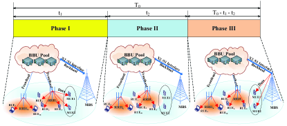
Figure 2: Frame structure and scheduling algorithm

• Phase I : During the time period of $\left[0,t_{1}\right]$ in each TTI, the RRH-alone with UEs-all scheme operates, where RRHs help the MBS serve the MUE, and the MBS benefits RRHs. Particularly, all $K$ RRHs serve $M$ RUEs and the single MUE in the typical RB, while the MBS remains idle. Since $K\geq M\!+\!1$ is satisfied, the interference between RUEs and the MUE can be suppressed by using distributed precoding in the BBU pool. Note that RRHs consume additional power for serving the MUE, which can be regarded as the payoff of the RRHs.

• Phase II : During the time period of $\left[t_{1},t_{1}\!+\!t_{2}\right]$ in each TTI, the RRH-alone with RUEs-only scheme operates, where all $K$ RRHs only serve the accessed $M$ RUEs, while the MBS remains idle and the corresponding MUE is not served. Since RRHs help the MBS to serve the MUE in Phase I, the MBS awards RRHs by staying idle at this phase; thus there is no inter-tier interference from the MBS to RUEs.

• Phase III : During the remaining time period of $\left[t_{1}\!+\!t_{2},T_{0}\right]$ in each TTI, the RRH-MBS with UEs-separated scheme operates, where RRHs and the MBS serve RUEs and the MUE, respectively. To mitigate the inter-tier interference, the fairness power control is utilized herein.

The H-CRAN architecture can support efficiently the contract-based interference coordination framework, in which the BBU pool manages all connected RRHs and accessed RUEs. The inter-tier interference coordination happens between the BBU pool and the MBS, which avoids the substantial overhead and capacity requirements between LPNs and MBSs of HetNets. Note that the advanced inter-tier interference collaboration scheme [13] and radio resource cooperative management techniques [15] can be used to replace the RRH-MBS with UEs-separated scheme at Phase III. To highlight characteristics of the proposed contract-based cooperative transmission framework and exploit performance gains resulting from contract-based game theory in H-CRANs, scheduling without coordinating the severe inter-tier interference is considered in the Phase III.

Remark: The BBU pool and the MBS have conflicting objectives in the aforementioned three schemes. RRHs want to have a longer $t_{2}$ because all RUEs can be served without inter-tier interference during Phase II. Alternatively, the MBS wants a longer $t_{1}$ because the MUE can be served by RRHs without its own power consumption. If both RRHs and the MBS can benefit from this presented transmission framework, they would cooperate with each other. Otherwise, it would lead to $t_{1}\!=\!t_{2}\!=0$, and ${t_{3}}={T_{0}}$ which devolves to the traditional transmission scheme enduring severe inter-tier interference. The core idea of the proposed framework is that two participants under information asymmetry, i.e., the BBU pool and MBS, establish a mutually beneficial relationship, which can be effectively modeled and optimized by using contract-based game theory.

III Optimal Contract Design under Complete CSI

It is preferred that BBU pool managing on all RRHs and RUEs act as the principal, due to the powerful capabilities of centralized cloud computing and large-scale cooperative processing. In the contract-based game model, the BBU pool as the principal designs a contract and offers it to the agent. The MBS as the agent decides to accept or reject the offered contract. Since the BBU pool and MBS are connected with an X2/S1 interface in H-CRANs, it is possible for them to exchange the corresponding individual CSI timely and completely. Thus, we can assume that the BBU pool can acquire the global and perfect CSI in this section.

III-A Rate-based Utility Definition

A rated-based utility function for the contract is considered in this paper to represent the SE performance of H-CRANs. Though more advanced precoding techniques can be utilized to provide better interference coordination performance with higher implementing complexities than ZF does, the ZF precoding technique is adopted in this paper to suppress the inter-RRH interference in the BBU pool because this common linear precoding can achieve performance close to the sum capacity bound with a relatively low complexity when the number of RUEs is sufficiently large in interference-limited H-CRAN systems [16].

• Phase I: Denote the received symbol power of $s_{m}$ and $s_{M\!+\!1}$ by $P_{C1}$ and $P_{M1}$, respectively. The sum transmission data rate of all RUEs, denoted by $R_{C1}$, and the data rate of the MUE, denoted by $R_{M1}$, can be expressed as

  $$R_{C1}\! =\!M\log\left(1\!+\!\frac{P_{C1}}{\sigma_{n}^{2}}\right),$$ (3)

  $$R_{M1}\! =\!\log\left(1\!+\!\frac{P_{M1}}{\sigma_{n}^{2}}\right),$$ (4)

  respectively. Defining $\mathbf{F}\!=\![\mathbf{G}^{T},\mathbf{f}_{M}^{T}]^{T}$, the expected total transmit power of the RRHs is constrained by

  $$\mathcal{E}\left\{\textup{tr}\left(\mathbf{F}\mathbf{F}^{H}\right)^{-1}\mathbf{\Lambda}\right\}\!\leq\!P_{\mathrm{max}},$$ (5)

  where $P_{\mathrm{max}}$ is the pre-defined allowable maximum transmit power, and $\mathbf{\Lambda}$ is an $(M\!+\!1)\times(M\!+\!1)$ diagonal matrix with the $(M\!+\!1)$-th diagonal element given by $P_{M1}$ and other diagonal elements given by $P_{C1}$. The transmit power constraint can be re-written as

  $$\textup{tr}\left(\mathbf{\tilde{D}}^{-\frac{1}{2}}\mathcal{E}\left\{(\mathbf{\tilde{H}}\mathbf{\tilde{H}}^{H})^{-1}\right\}\mathbf{\tilde{D}}^{-\frac{1}{2}}\mathbf{\Lambda}\right)\!\leq\!P_{\mathrm{max}},$$ (6)

  where $\mathbf{\tilde{D}}\!=\!\mathbf{diag}\left(\upsilon_{m},\ldots,\upsilon_{M+1}\right)$ is an $(M\!+\!1)\times(M\!+\!1)$ diagonal matrix with $\mathbf{\tilde{H}}\!=\![\mathbf{H}^{T},\mathbf{h}_{f}^{T}]^{T}$, where $\mathbf{h}_{f}$ is a $1\times K$ Gaussian vector with zero means and unity variances. As $\tilde{\mathbf{H}}\tilde{\mathbf{H}}^{H}\sim\mathcal{W}(M\!+\!1,\mathbf{I}_{M\!+\!1})$ is an $(M\!+\!1)\times(M\!+\!1)$ central complex Wishart matrix with $K(K\!>\!M\!+\!1)$ degrees of freedom, (6) can be written as

  $$\sum_{m=1}^{M}\frac{P_{C1}}{(K\!-\!M\!-\!1)\upsilon_{m}}\!+\!\frac{P_{M1}}{(K\!-\!M\!-\!1)\upsilon_{M\!+\!1}}\!\leq\!P_{\mathrm{max}}.$$ (7)

• Phase II: Denote the received symbol power of $s_{m}$ by $P_{C2}$, and the sum rate of all RUEs can be expressed as

  $$R_{C2}\!=\!M\log\left(1\!+\!\frac{P_{C2}}{\sigma_{n}^{2}}\right),$$ (8)

  where the long-term average transmit power is similarly constrained by

  $$\mathcal{E}\bigg{\{}P_{C2}\mathrm{tr}\left(\mathbf{G}\mathbf{G}^{H}\right)^{-1}\bigg{\}}=\sum_{m\!=\!1}^{M}\frac{P_{C2}}{\upsilon_{m}\left(K\!-\!M\right)}\!\leq\!P_{\mathrm{max}}.$$ (9)

  Since there is no inter-tier interference from the MBS to the desired RUEs due to the silent MUE, $P_{C2}$ would be always set at the maximum value $P_{C2}\!=\!\frac{\left(K\!-\!M\right)P_{\mathrm{max}}}{\varepsilon_{1}}$ to optimize the sum rate, where $\varepsilon_{1}\!=\!\sum_{m=1}^{M}\frac{1}{\upsilon_{m}}$.

• Phase III: Denote the transmit power of the MBS and the RRH by $P_{B}$ and $P_{C3}$, respectively. Under the fairness power control algorithm[30], $P_{C3}$ and $P_{B}$ are derived from

  $$\{P_{C3},{P_{B}}\}\! =\!\arg\mathop{\max}\limits_{P_{C3},P_{B}}\min\left\{{{R_{C3}},{R_{M3}}}\right\},$$ (10)

  $$s.t.\quad 0\!\leq\!P_{C3}\!\leq\!P_{\rm{max}},\thinspace 0\!\leq\!P_{B}\!\leq\!P_{\rm{max}}.$$ (11)

  The sum rate of all RUEs, denoted by $R_{C3}$, and the data rate of the MUE, denoted by $R_{M3}$, can be expressed as

  $${R_{C3}}=\sum\limits_{m=1}^{M}{\log}\left({1+\frac{{{P_{C3}}}}{{|{f_{Bm}}{|^{2}}{P_{B}}+\sigma_{n}^{2}}}}\right),$$ (12)

  $${R_{M3}}=\log\left({1+\frac{{|{g_{B}}{|^{2}}{P_{B}}}}{{{P_{C3}}{{\bf{f}}_{M}}{{\bf{G}}^{H}}{{\left({{\bf{G}}{{\bf{G}}^{H}}}\right)}^{-2}}{\bf{Gf}}_{M}^{H}+\sigma_{n}^{2}}}}\right),$$ (13)

respectively.

The rate-based utility of the BBU pool is defined as the sum rate in each TTI obtained by adopting the proposed framework compared with the traditional scheme in Phase III, which is given by

$${U_{C}}={t_{1}}{R_{C1}}+\left({{T_{0}}-{t_{1}}-{t_{3}}}\right){R_{C2}}-\left({{T_{0}}-{t_{3}}}\right){R_{C3}}.$$ (14)

Further, the data rate-based utility of the MBS during each TTI can be expressed as

$${U_{M}}={t_{1}}{R_{M1}}+{t_{3}}{R_{M3}}.$$ (15)

III-B Contract Design under Perfect CSI

To make the contract feasible under complete CSI, the principal should ensure that the agent obtains at least the reservation utility value that it would get by accepting this contract. Such a constraint is known as being individual rational (IR), which has the following definition.

• (Individual Rational) A contract with the item $\left({{t_{1}},{t_{3}},{P_{M1}},{P_{C1}}}\right)$ is individual rational if the rate-based utility that the agent obtains is larger than the reservation utility ${u}$, i.e.,

  $${t_{1}}{R_{M1}}+{t_{3}}{R_{M3}}\geq u={T_{0}}{R_{M3}}.$$ (16)

Since the principal desires to obtain a maximal profit from the contract, the optimal contract $\left({t_{1}^{*},t_{3}^{*},P_{M1}^{*},P_{C1}^{*}}\right)$ can be obtained from

$$\begin{split}\left({t_{1}^{*},t_{3}^{*},P_{M1}^{*},P_{C1}^{*}}\right)&=\arg\mathop{\max}\limits_{{t_{1}},{t_{3}},{P_{M1}},{P_{C1}}}\bigg{\{}t_{1}R_{C1}+\\ &\left({{T_{0}}-{t_{1}}-{t_{3}}}\right){R_{C2}}-\left({{T_{0}}-{t_{3}}}\right)R_{C3}\bigg{\}},\\ s.t.\quad&{t_{1}}{R_{M1}}+{t_{3}}{R_{M3}}\geq{T_{0}}{R_{M3}},\\ &{t_{3}}\geq 0,{t_{1}}\geq 0,{T_{0}}-{t_{1}}-{t_{3}}\geq 0,\\ &\frac{P_{C1}}{\left(K\!-\!M\!-\!1\right)\varepsilon_{1}}\!+\!\frac{P_{M1}}{\left(K\!-\!M\!-\!1\right)\upsilon_{M\!+\!1}}\!\leq\!P_{\rm{max}}.\end{split}$$ (17)

Lemma 1

Under complete CSI, the contract $\left({t_{1}^{*},t_{3}^{*},P_{M1}^{*},P_{C1}^{*}}\right)$ that maximizes the rate-based utility of the BBU pool satisfies the following conditions:

$$t_{1}^{*}R_{M1}^{*}-\left({{T_{0}}-t_{3}^{*}}\right)R_{M3}^{*}=0,$$ (18)

$$t_{3}^{*}=0,$$ (19)

$$\frac{P^{*}_{C1}}{\left(K\!-\!M\!-\!1\right)\varepsilon_{1}}\!+\!\frac{P^{*}_{M1}}{\left(K\!-\!M\!-\!1\right)\upsilon_{M\!+\!1}}\!=\!P_{\mathrm{max}}.$$ (20)

Proof:

See Appendix A. ∎

Remark: Lemma 1 indicates that the MBS will obtain zero utility gain from the contract, which is not unexpected since the BBU pool will maximize its own utility with the minimal payoff. Moreover, the time period of Phase III would be zero when the contract is accepted by the MBS. Otherwise, the contract is rejected.

Once the optimal contract is accepted, the objective function depends only on $P_{M1}$, and the computational complexity for obtaining $P^{*}_{M1}$ is acceptable with numerical methods, which is provided in Algorithm 1. Once $P^{*}_{M1}$ is obtained, $t_{1}^{*}$ and $P^{*}_{C1}$ can be directly determined.

TABLE II: Algorithm 1: one-dimensional search for $P_{M1}^{*}$ under perfect CSI

Input: $P_{M1}^{(1)}$, $P_{M1}^{(2)}$, where $P_{M1}^{(1)},P_{M2}^{(2)}\in[0,(K\!-\!M\!-\!1)\upsilon_{M+1}P_{\rm{max}}]$

satisfy $P_{M1}^{(2)}>P_{M1}^{(1)}$, $\varsigma_{1}=\frac{\partial{U}_{C}}{\partial P_{M1}}\big{|}_{P_{M1}=P_{M1}^{(1)}}<0$,

and $\varsigma_{2}=\frac{\partial{U}_{C}}{\partial P_{M1}}\big{|}_{P_{M1}=P_{M1}^{(2)}}>0$.

Initialize: $U_{C}^{(1)}$, $U_{C}^{(2)}$ by substituting $P_{M1}^{(1)}$ and $P_{M1}^{(2)}$ into (14), respectively.

$k=1$, error $\epsilon\!>\!0$.

Repeat until convergence:

Calculate:

$s=\frac{3[U_{C}^{(2)}-U_{C}^{(1)}]}{P_{M1}^{(2)}-P_{M1}^{(1)}}$, $z=s-\varsigma_{1}-\varsigma_{2}$,  $w=\sqrt{z^{2}-\varsigma_{1}\varsigma_{2}}$,

$\bar{P}_{M1}=P_{M1}^{(1)}+(P_{M1}^{(2)}-P_{M1}^{(1)})\left(1-\frac{\varsigma_{2}+w+z}{\varsigma_{2}-\varsigma_{1}+2w}\right)$.

If $|P_{M1}^{(2)}-P_{M1}^{(1)}|\leq\epsilon$

Termination criterion is satisfied.

Else

Calculate $\bar{U}_{C}$ and $\varsigma=\frac{\partial U_{C}}{\partial P_{M1}}\big{|}_{P_{M1}=\bar{P}_{M1}}$ by substituting $\bar{P}_{M1}$ into (14).

If $\varsigma=0$

Termination criterion is satisfied.

Else

If $\varsigma<0$

$P_{M1}^{(1)}=\bar{P}_{M1}$, $U_{C}^{(1)}=\bar{U}_{C}$ and $\varsigma_{1}=\varsigma$,

If $\varsigma>0$

$P_{M1}^{(2)}=\bar{P}_{M1}$, $U_{C}^{(2)}=\bar{U}_{C}$ and $\varsigma_{2}=\varsigma$,

$k\!=\!k\!+\!1$.

Remark: Algorithm 1 is based on the spline interpolation method, whose computational complexity is mainly determined by the number of iterations. In this case, the computational complexity can be expressed as $O\left(k\right)$, where $k$ denotes the number of iterations. Note that $k$ depends on the error convergence parameter $\epsilon$ and the initial configuration of $P_{M1}$ critically; thus it is important to choose proper initial $P_{M1}$ to promote the convergence of the algorithm.

Of course, complete and perfect CSI cannot usually be achieved in practice. In practical H-CRANs, CSI must be estimated and quantified, and is not error-free or delay-free. In the following section, we consider the impact of the imperfect CSI on the contract-based framework, where the principal can only acquire partial and non-ideal CSI via channel estimation.

IV Contract Design under Practical Channel Estimation

In order to enable the BBU pool to acquire the downlink instantaneous CSI, an uplink training design is considered, which is based on the channel reciprocity in the time division duplex (TDD) mode. It is assumed that the fronthaul and backhaul are non-constrained and ideal, while the radio access links are non-ideal.

IV-A Uplink Training Design and Channel Estimation

Let $\bm{\psi}_{m}$ denote the training sequence transmitted from the $m$-th RUE to the corresponding RRH, and $\bm{\psi}_{M\!+\!1}$ represents the training sequence from the MUE to the MBS. All $\bm{\psi}_{m}$’s have the $N$($>M$) symbol length. $\|\bm{\psi}_{m}\|^{2}\!=\!NP_{s}$ and $\|\bm{\psi}_{M\!+\!1}\|^{2}\!=\!NP_{b}$, where $P_{s}$ and $P_{b}$ are the training power of the RUEs and MUE, respectively. Moreover, $\mathbf{\Psi}\!=\!\left[\bm{\psi}_{1},\bm{\psi}_{2},\ldots,\bm{\psi}_{M}\right]$ satisfies $\mathbf{\Psi}^{H}\mathbf{\Psi}\!=\!NP_{s}\mathbf{I}_{M}$ and $\mathbf{\Psi}^{H}\bm{\psi}_{M\!+\!1}\!=\!\mathbf{0}_{M}$. During the training stage in the uplink, all RUEs and the MUE transmit their own training sequences simultaneously, and the observations at the $k$-th RRH can be expressed as

$$\mathbf{x}_{k}\!=\!\sum_{m\!=\!1}^{M}g_{mk}\bm{\psi}_{m}\!+\!f_{kM}\bm{\psi}_{M\!+\!1}\!+\!\mathbf{w}_{k},$$ (21)

where $\mathbf{w}_{k}$ is an $N\!\times\!1$ dimensional AWGN vector with covariance $\sigma_{n}^{2}\mathbf{I}_{N}$. The least-squares estimate (LSE) of the channel coefficient between the $k$-th RRH and $m$-th RUE $g_{mk}$, denoted by $\hat{g}_{mk}$, can be expressed as

$$\hat{g}_{mk}\!=\!\frac{\bm{\psi}^{H}_{m}}{\|\bm{\psi}_{m}\|^{2}}\mathbf{x}_{k},$$ (22)

and the LSE of the channel coefficient between $k$-th RRH and MUE $f_{kM}$ is

$$\hat{f}_{kM}\!=\!\frac{\bm{\psi}^{H}_{M\!+\!1}}{\|\bm{\psi}_{M\!+\!1}\|^{2}}\mathbf{x}_{k}.$$ (23)

Similarly, the MBS observes

$$\mathbf{x}_{B}\!=\!\bm{\psi}_{M\!+\!1}g_{B}\!+\sum_{m\!=\!1}^{M}\bm{\psi}_{m}f_{Bm}\!+\!\mathbf{w}_{B},$$ (24)

where $\mathbf{w}_{B}$ is an $N\!\times\!1$ dimensional AWGN vector with covariance $\sigma_{n}^{2}\mathbf{I}_{N}$. The LSEs of $g_{B}$ and $f_{Bm}$ are

$$\hat{g}_{B}\!=\!\frac{\bm{\psi}_{M\!+\!1}^{H}}{\|\bm{\psi}_{M\!+\!1}\|^{2}}\mathbf{x}_{B},$$ (25)

$$\hat{f}_{Bm}\!=\!\frac{\bm{\psi}_{m}^{H}}{\|\bm{\psi}_{m}\|^{2}}\mathbf{x}_{B},$$ (26)

respectively. The mean-square errors (MSEs) of $\hat{g}_{mk}$ and $\hat{f}_{Bm}$, denoted by $\delta_{mk}$ and $\delta_{Bm}$, are equal and can be written as

$$\delta_{mk}\!=\!\delta_{Bm}\!=\frac{\mathcal{E}\left\{\|\bm{\psi}^{H}_{m}\mathbf{w}_{k}\|^{2}\right\}}{\|\bm{\psi}_{m}\|^{2}}\!=\!\frac{\mathcal{E}\left\{\|\bm{\psi}^{H}_{M\!+\!1}\mathbf{w}_{k}\|^{2}\right\}}{\|\bm{\psi}_{M\!+\!1}\|^{2}}\!=\!\underbrace{\frac{\sigma_{n}^{2}}{NP_{s}}}_{\delta_{1}}.$$ (27)

Similarly, the MSEs of $\hat{g}_{B}$ and $\hat{f}_{kM}$, denoted by $\delta_{B}$ and $\delta_{kM}$, can equivalently be written as

$$\delta_{B}\!=\!\delta_{kM}\!=\!\underbrace{\frac{\sigma_{n}^{2}}{NP_{b}}}_{\delta_{2}}.$$ (28)

IV-B Contract Design under Imperfect CSI

For notational simplicity, we define $\hat{R}_{C1}$, $\hat{R}_{M1}$, $\hat{R}_{C2}$, $\hat{R}_{C}$, and $\hat{R}_{M}$ under imperfect CSI to be compatible with the corresponding data rates $R_{C1}$, $R_{M1}$, $R_{C2}$, $R_{C}$, and $R_{M}$ under complete CSI. These transmission data rates under imperfect CSI are characterized in the following lemma.

Lemma 2

The transmission data rates for all RUEs and the MUE at the three phases are given as follows.

Phase I: The sum transmission data rate of all RUEs and the data rate of the MUE are given by

$$\hat{R}_{C1}\!=\!M$$

$$\log\!\left(1\!+\!\frac{P_{C1}}{\delta_{1}P_{C1}\!\!\displaystyle\sum_{m\!=\!1}^{M}\!\!\left[\hat{\mathbf{F}}\hat{\mathbf{F}}^{H}\right]^{-1}_{m,m}\!\!\!+\!\delta_{2}P_{M1}\left[\hat{\mathbf{F}}\hat{\mathbf{F}}^{H}\right]^{-1}_{M\!+\!1,M\!+\!1}\!+\!\sigma_{n}^{2}}\right),$$ (29)

$$\hat{R}_{M1}\!=\!$$

$$\log\!\left(1\!+\!\frac{P_{M1}}{\delta_{1}P_{C1}\!\!\displaystyle\sum_{m\!=\!1}^{M}\!\!\left[\hat{\mathbf{F}}\hat{\mathbf{F}}^{H}\right]^{-1}_{m,m}\!\!\!+\!\delta_{2}P_{M}\left[\hat{\mathbf{F}}\hat{\mathbf{F}}^{H}\right]^{-1}_{M\!+\!1,M\!+\!1}\!+\!\sigma_{n}^{2}}\right),$$ (30)

respectively, where the total transmit power is constrained by

$$\sum_{m\!=\!1}^{M}\frac{P_{C1}}{\left(K\!-\!M\!-\!1\right)\left(\upsilon_{m}\!+\!\delta_{1}\right)}\!+\!\frac{P_{M1}}{\left(K\!-\!M\!-\!1\right)\left(\upsilon_{M\!+\!1}\!+\!\delta_{2}\right)}\!\leq\!P_{\mathrm{max}}.$$ (31)

Phase II: The sum rate of all RUEs can be expressed as

$$\hat{R}_{C2}\!=\!M\log\left(1\!+\!\frac{P_{C2}}{\delta_{1}P_{C2}\mathrm{tr}\!\bigg{\{}\left[\hat{\mathbf{G}}\hat{\mathbf{G}}^{H}\right]^{-1}\bigg{\}}\!+\!\sigma_{n}^{2}}\right),$$ (32)

where the total transmit power is constrained by

$$\sum_{m\!=\!1}^{M}\frac{P_{C2}}{\left(\upsilon_{m}\!+\!\delta_{1}\right)\left(K\!-\!M\right)}\!\leq\!P_{\mathrm{max}}.$$ (33)

Note that RRHs prefer to achieve the maximal sum rate, and thus $P_{C2}$ would always be set at the maximum value as $P_{C2}\!=\!\frac{\left(K\!-\!M\right)P_{\mathrm{max}}}{\varepsilon_{2}}$ with $\varepsilon_{2}\!=\!\sum_{m=1}^{M}\frac{1}{\upsilon_{m}\!+\!\delta_{1}}$.

Phase III: The sum rate of all RUEs and the data rate of the MUE are given by

$$\hat{R}_{C3}$$

$$\!=\!\sum_{m\!=\!1}^{M}\log\left(1\!+\!\frac{P_{C3}}{\delta_{1}P_{C3}\mathrm{tr}\!\bigg{\{}\left[\hat{\mathbf{G}}\hat{\mathbf{G}}^{H}\right]^{-1}\bigg{\}}\!+\!|f_{Bm}|^{2}P_{B}\!+\!\sigma_{n}^{2}}\right),$$ (34)

$$\hat{R}_{M3}\!=\!\log\left(1\!+\!\frac{|g_{B}|^{2}P_{B}}{P_{C3}\mathbf{f}\hat{\mathbf{G}}^{H}\left(\hat{\mathbf{G}}\hat{\mathbf{G}}^{H}\right)^{-2}\hat{\mathbf{G}}\mathbf{f}^{H}\!+\!\sigma_{n}^{2}}\right),$$ (35)

respectively. With the same power control algorithm as under perfect CSI, $P_{C3}$ and $P_{B}$ under the fairness power control can be achieved by

$$\{P_{C3},{P_{B}}\}\! =\!\arg\mathop{\max}\limits_{P_{C3},P_{B}}\min\left\{{{\hat{R}_{C3}},{\hat{R}_{M3}}}\right\},$$

$$s.t.\quad 0\!\leq\!P_{C3}\!\leq\!P_{\rm{max}},\thinspace 0\!\leq\!P_{B}\!\leq\!P_{\rm{max}}.$$ (36)

Proof:

See Appendix B. ∎

The BBU pool can acquire the estimated CSI of the RRH-RUE and RRH-MUE links, and it cannot estimate CSI of the MBS-MUE link, i.e., ${\left|{{g_{B}}}\right|^{2}}$, which results in information asymmetry. In order to design the optimal contract, an incentive compatible (IC) constraint is presented according to the revelation principle [31]. It is assumed that ${\left|{{g_{B}}}\right|^{2}}$ has $L$ potential quantified values and the set containing those values is denoted by $\Xi=\left\{{{\xi_{1}},{\xi_{2}},\ldots,{\xi_{L}}}\right\}$. Without loss of generality, we further assume that ${\xi_{1}}<{\xi_{2}}<\ldots<{\xi_{L}}$. The IC constraint can be defined as follows.

• (Incentive Compatible) A contract is incentive compatible if the agent with channel coefficients of the MBS-MUE link ${\left|{{g_{B}}}\right|^{2}}={\xi_{l}}$ prefers to choose the contract item $(t_{1}^{l},t_{3}^{l},P_{M1},P_{C1})$ designed specifically for its own type, i.e.,

  $$t_{1}^{l}\hat{R}_{M1}+t_{3}^{l}\hat{R}_{M3}^{l}\geq t_{1}^{l^{\prime}}\hat{R}_{M1}+t_{3}^{l^{\prime}}\hat{R}_{M3}^{l},\forall l,l^{\prime}\in\left\{{1,2,\ldots,L}\right\}.$$ (37)

On the other hand, the IR constraint under partial CSI is given by the following definition.

• (Individual Rational) A contract is individual rational if the rate-based utility that the agent with ${\left|{{g_{B}}}\right|^{2}}={\xi_{l}}$ obtains by choosing the contract item $(t_{1}^{l},t_{3}^{l},P_{M1},P_{C1})$ is larger than the reservation utility ${u_{l}}$ , i.e.,

  $$t_{1}^{l}\hat{R}_{M1}+t_{3}^{l}\hat{R}_{M3}^{l}\geq{u_{l}}={T_{0}}\hat{R}_{M3}^{l},\forall l\in\left\{{1,2,\ldots,L}\right\},$$ (38)

  where $t_{1}^{l}$ and $t_{3}^{l}$ are the time duration of Phase I and Phase III intended for the agent with ${\left|{{g_{B}}}\right|^{2}}={\xi_{l}}$, respectively, and $\hat{R}_{M3}^{l}$ is calculated by (35) under ${\left|{{g_{B}}}\right|^{2}}={\xi_{l}}$.

Since the BBU pool can obtain the knowledge of the statistical parameters and the distributions of random variables by using appropriate learning and fitting methods, we assume that the BBU pool can acquire the probability density function (pdf) of $z\!=\!|f_{Bm}|^{2}$, the set ${\Xi}=\left\{{{\xi_{1}},{\xi_{2}},\ldots,{\xi_{L}}}\right\}$, and the variable ${q_{l}}$ denoting the possibility of ${\left|{{g_{B}}}\right|^{2}}={\xi_{l}}$. Obviously, ${q_{l}}\in\left[{0,1}\right]$ and $\sum\limits_{l\in\left\{{1,2,\ldots,L}\right\}}{{q_{l}}}=1$.

Hence, when the contract is accepted by the MBS with ${\left|{{g_{B}}}\right|^{2}}={\xi_{l}}$, the rate-based utility in the BBU pool can be written as

$${U_{C}}= t_{1}^{l}\hat{R}_{C1}+\left({{T_{0}}-t_{1}^{l}-t_{3}^{l}}\right){{\hat{R}}_{C2}}$$

$$-\left({{T_{0}}-t_{3}^{l}}\right)\int_{z}p\left(z\right){{\hat{R}}_{C3}}dz.$$ (39)

Similarly, the rate-based utility in the MBS can be obtained by

$${U_{M}}=t_{1}^{l}\hat{R}_{M1}+t_{3}^{l}\hat{R}_{M3}^{l}.$$ (40)

Then the optimal contract with imperfect CSI can be obtained by solving the following optimization problem:

$$\mathop{\max}\limits_{\left\{{\left({t_{1}^{l},t_{3}^{l},{P_{M1}},{P_{C1}}}\right),\forall l\in\left\{{1,2,\ldots,L}\right\}}\right\}}$$

$${\rm{}}\sum\limits_{l\in\left\{{1,2,\ldots,L}\right\}}\!\!{{q_{l}}\left[{t_{1}^{l}{{\hat{R}}_{C1}}+\left({{T_{0}}-t_{1}^{l}-t_{3}^{l}}\right){{\hat{R}}_{C2}}-\left({{T_{0}}-t_{3}^{l}}\right){{\hat{R}}_{C3}}}\right]}$$ (41)

$$s.t.\quad t_{1}^{l}\hat{R}_{M1}+t_{3}^{l}\hat{R}_{M3}^{l}\geq{T_{0}}\hat{R}_{M3}^{l},\forall l\!\in\!\left\{{1,2,\ldots,L}\right\},$$ (42)

$$\quad\quad t_{1}^{l}\hat{R}_{M1}+t_{3}^{l}\hat{R}_{M3}^{l}\geq t_{1}^{l^{\prime}}\hat{R}_{M1}+t_{3}^{l^{\prime}}\hat{R}_{M3}^{l},$$

$$\quad\quad\forall l,l^{\prime}\in\left\{{1,2,\ldots,L}\right\},$$ (43)

$$\quad\quad t_{3}^{l}\geq 0,t_{1}^{l}\geq 0,{T_{0}}-t_{1}^{l}-t_{3}^{l}\geq 0,\forall l\in\left\{{1,2,\ldots,L}\right\},$$ (44)

$$\quad\quad{P_{M1}}\geq 0,{P_{C1}}\geq 0,$$ (45)

$$\quad\quad\frac{P_{C1}}{\left(K\!-\!M\!-\!1\right)\varepsilon_{2}}+\frac{{{P_{M1}}}}{\left(K-M-1\right)(\upsilon_{M+1}+\delta_{2})}\leq P_{\rm{max}}.$$ (46)

The above optimization problem can be further transformed to

$$\mathop{\max}\limits_{\left\{{\left({t_{3}^{l},{P_{M1}},{P_{C1}}}\right),\forall l\in\left\{{1,2,\ldots,L}\right\}}\right\}}\quad U_{{C_{\left\{{\left({t_{3}^{l},{P_{M1}},{P_{C1}}}\right),\forall l\in\left\{{1,2,\ldots,L}\right\}}\right\}}}}^{*}$$ (47)

$$s.t.\quad 0\leq t_{3}^{1}\leq t_{3}^{2}\leq\cdots\leq t_{3}^{L},$$ (48)

$$\quad\quad{T_{0}}-\tilde{t}_{1}^{l}-t_{3}^{l}\geq 0,\forall l\in\left\{{1,2,\ldots,L}\right\},$$ (49)

$$\quad\quad{P_{M1}}\geq 0,{P_{C1}}\geq 0,$$ (50)

$$\quad\quad\frac{P_{C1}}{\left(K\!-\!M\!-\!1\right)\varepsilon_{2}}+\frac{{{P_{M1}}}}{\left(K-M-1\right)(\upsilon_{M+1}+\delta_{2})}\leq P_{\rm{max}},$$ (51)

where

$$U_{{C_{\left\{{\left({t_{3}^{l},{P_{M1}},{P_{C1}}}\right),\forall l\in\left\{{1,2,\ldots,L}\right\}}\right\}}}}^{*}$$

$$=\left[{{{\hat{R}}_{C1}}-{{\hat{R}}_{C2}}}\right]\sum\limits_{l\in\left\{{1,2,\ldots,L}\right\}}{{q_{l}}}\tilde{t}_{1}^{l}-\hat{R}\sum\limits_{l\in\left\{{1,2,\ldots,L}\right\}}{{q_{l}}}t_{3}^{l}+{T_{0}}\hat{R},$$ (52)

$$\hat{R}={\hat{R}_{C2}}-{\hat{R}_{C3}},\thinspace\tilde{t}_{1}^{1}=\frac{{{u_{L}}-t_{3}^{1}\hat{R}_{M3}^{1}}}{{{{\hat{R}}_{M1}}}},$$ (53)

$$\tilde{t}_{1}^{l}=\frac{1}{{{{\hat{R}}_{M1}}}}\left[{{u_{L}}-t_{3}^{1}\hat{R}_{M3}^{1}+\sum\limits_{i=2}^{l}{\hat{R}_{M3}^{i}\left({t_{3}^{i-1}-t_{3}^{i}}\right)}}\right],$$

$$\forall l\in\left\{{2,\ldots,L}\right\}.$$ (54)

Note that the rate-based utility optimization in (47) with constraints (48)–(51) cannot always be solved in closed-form, which makes it difficult to design the optimal contract directly. Nevertheless, once the pdf of each random variable is determined, the optimal contract can be achieved according to the following Algorithm 2.

TABLE III: Algorithm 2: one-dimensional search for $P_{M1}^{*}$ under imperfect CSI

Input: $P_{M1}^{(1)}$, $P_{M1}^{(2)}$, where $P_{M1}^{(1)},P_{M2}^{(2)}\in[0,(K\!-\!M\!-\!1)(\upsilon_{M+1}+\delta_{2})P_{\rm{max}}]$ satisfy $P_{M1}^{(2)}>P_{M1}^{(1)}$,

$\varsigma_{1}=\frac{\partial{U}_{C}^{*}}{\partial P_{M1}}\big{|}_{P_{M1}=P_{M1}^{(1)}}<0$, and $\varsigma_{2}=\frac{\partial{U}_{C}^{*}}{\partial P_{M1}}\big{|}_{P_{M1}=P_{M1}^{(2)}}>0$.

Initialize: $U_{C}^{*(1)}$, $U_{C}^{*(2)}$ by substituting $P_{M1}^{(1)}$ and $P_{M1}^{(2)}$ into (IV-B), respectively,

$k=1$, error $\epsilon\!>\!0$.

Repeat until convergence:

Calculate:

$s=\frac{3[U_{C}^{*(2)}-U_{C}^{*(1)}]}{P_{M1}^{(2)}-P_{M1}^{(1)}}$, $z=s-\varsigma_{1}-\varsigma_{2}$,  $w=\sqrt{z^{2}-\varsigma_{1}\varsigma_{2}}$, $\bar{P}_{M1}=P_{M1}^{(1)}+(P_{M1}^{(2)}-P_{M1}^{(1)})\left(1-\frac{\varsigma_{2}+w+z}{\varsigma_{2}-\varsigma_{1}+2w}\right)$.

If $|P_{M1}^{(2)}-P_{M1}^{(1)}|\leq\epsilon$

Termination criterion is satisfied.

Else

Calculate $\bar{U}_{C}$ and $\varsigma=\frac{\partial U_{C}^{*}}{\partial P_{M1}}\big{|}_{P_{M1}=\bar{P}_{M1}}$ by substituting $\bar{P}_{M1}$ into (IV-B).

If $\varsigma=0$

Termination criterion is satisfied.

Else

If $\varsigma<0$

$P_{M1}^{(1)}=\bar{P}_{M1}$, $U_{C}^{*(1)}=\bar{U}_{C}$ and $\varsigma_{1}=\varsigma$,

If $\varsigma>0$

$P_{M1}^{(2)}=\bar{P}_{M1}$, $U_{C}^{*(2)}=\bar{U}_{C}$ and $\varsigma_{2}=\varsigma$,

$k\!=\!k\!+\!1$.

Remark: The computational complexity of Algorithm 2 is similar to that of Algorithm 1.

IV-C Discussion with the Sufficiently Large $K$

In this subsection, we consider the case in which the number of RRHs is large. It is assumed that each radio channel coefficient has a complex Gaussian distribution with mean zero. According to the Law of Large Numbers, we have the following approximations:

$$\frac{1}{K}\hat{\mathbf{G}}\hat{\mathbf{G}}^{H}\!\rightarrow\!\mathbf{D}\!+\!\delta_{1}\mathbf{I}_{M},\thinspace\frac{1}{K}\hat{\mathbf{F}}\hat{\mathbf{F}}^{H}\!\rightarrow\!\mathrm{diag}\left[\mathbf{D}\!+\!\delta_{1}\mathbf{I}_{M},\left(\upsilon_{M+1}\!+\!\delta_{2}\right)\right].$$ (55)

• When the number of RRHs is sufficiently large, the transmission data rates of all RUEs and the MUE at three phases under imperfect CSI can be rewritten as

  $$\tilde{R}_{C1}\! =\!M\log\left(1\!+\!\frac{P_{C1}}{\frac{\delta_{1}P_{C1}}{K\varepsilon_{2}}\!+\!\frac{\delta_{2}P_{M}}{K\left(\upsilon_{M+1}\!+\!\delta_{2}\right)}\!+\!\sigma_{n}^{2}}\right),$$ (56)

  $$\tilde{R}_{M1}\! =\!\log\left(1\!+\!\frac{P_{M1}}{\frac{\delta_{1}P_{C1}}{K\varepsilon_{2}}\!+\!\frac{\delta_{2}P_{M1}}{K\left(\upsilon_{M+1}\!+\!\delta_{2}\right)}\!+\!\sigma_{n}^{2}}\right),$$ (57)

  $$\tilde{R}_{C2}\! =\!M\log\left(1\!+\!\frac{P_{C2}}{\frac{\delta_{1}P_{C2}}{K\varepsilon_{2}}\!+\!\sigma_{n}^{2}}\right),$$ (58)

  $$\tilde{R}_{C3}\! =\!\sum_{m\!=\!1}^{M}\log\left(1\!+\!\frac{P_{C3}}{\frac{\delta_{1}P_{C3}}{K\varepsilon_{2}}\!+\!|f_{Bm}|^{2}P_{B}\!+\!\sigma_{n}^{2}}\right),$$ (59)

  $$\tilde{R}_{M3}\! =\!\log\left(1\!+\!\frac{|g_{B}|^{2}P_{B}}{\frac{\upsilon_{M+1}P_{C3}}{K\varepsilon_{2}}\!+\!\sigma_{n}^{2}}\right).$$ (60)

Eqs. (56)–(60) in Definition 4 can be derived directly by substituting (55) into the transmission data rates in Lemma 2. Based on Definition 4, the optimal contract design can be derived via the following lemma when the number of RRHs is sufficiently large.

Lemma 3

For a sufficiently large $K$ under imperfect CSI, once the contract is accepted by the agent, the optimal $t_{3}^{l}$, $P_{C1}^{*}$, and $P_{M1}^{*}$ follow

$$t_{3}^{l}\!=\!0,l=1,\ldots,L-1,$$ (61)

$$t_{3}^{L}\!=\!\begin{cases}T_{0}&{{\tilde{R}}_{M1}}({{\tilde{R}}_{C2}}-{{\tilde{R}}_{C3}})<\tilde{R}_{M3}^{L}({{\tilde{R}}_{C2}}-{{\tilde{R}}_{C1}}),\\ [0,T_{0}]&{{\tilde{R}}_{M1}}({{\tilde{R}}_{C2}}-{{\tilde{R}}_{C3}})=\tilde{R}_{M3}^{L}({{\tilde{R}}_{C2}}-{{\tilde{R}}_{C1}}),\\ 0&{{\tilde{R}}_{M1}}({{\tilde{R}}_{C2}}-{{\tilde{R}}_{C3}})>\tilde{R}_{M3}^{L}({{\tilde{R}}_{C2}}-{{\tilde{R}}_{C1}}),\end{cases}$$ (62)

$$\frac{P_{C1}^{*}}{\left(K\!-\!M\!-\!1\right)\varepsilon_{2}}\!+\!\frac{P_{M1}^{*}}{\left(K\!-\!M\!-\!1\right)(\upsilon_{M\!+\!1}\!+\!\delta_{2})}\!=\!P_{\mathrm{max}}.$$ (63)

Proof:

See Appendix C. ∎

V Numerical Results

In this section, Monte Carlo simulations are provided to evaluate the performances of the proposed contract-based interference coordination framework in H-CRANs numerically. All the fast fading channel coefficients are generated as independent complex Gaussian random variables with zero means and unit variances. The large-scale fading coefficients $\upsilon_{m}$ ($m=1,\ldots,(M+1)$) are modeled as $\upsilon_{m}\!=\!z_{m}/(r_{m}/r_{0})^{v}$, where $z_{m}$ is log-normal random variable with standard deviation $8\thinspace\textup{dB}$, $r_{m}$ is the distance between the $m$-th UE and RRHs, $r_{0}$ is set to be $100$ meters, and $v\!=\!3.8$ is the path loss exponent. The other common parameters are set at $P_{\mathrm{max}}\!=\!1$, $T_{0}\!=\!1$, $M=4$ and $N\!=\!10$; thus the signal-to-noise ratio (SNR) is given by $\textup{SNR}\!=\!\frac{P_{\rm{max}}}{\sigma_{n}^{2}}\!=\!\frac{1}{\sigma_{n}^{2}}$. Totally $10^{5}$ Monte-Carlo runs are used for the average calculations. Two baselines are considered in this paper:

• Frequency reuse with power control (FRPC): RRHs and the MBS reuse the same RB, and the transmit powers are determined according to the fairness power control adopted for the proposed CICF in Phase III:

  $$\{P_{C3},{P_{B}}\}\! =\!\arg\mathop{\max}\limits_{P_{C3},P_{B}}\min\left\{{{R_{C3}},{R_{M3}}}\right\},$$

  $$s.t.\quad 0\!\leq\!P_{C3}\!\leq\!P_{\rm{max}},\thinspace 0\!\leq\!P_{B}\!\leq\!P_{\rm{max}}.$$

• Time domain interference cancelation (TDIC): RRHs and the MBS transmit separately in the different time phases, where the transmission duration allocated to RRHs and the MBS are $t_{R}$ and $t_{M}$, respectively, and they satisfy the relationship with $t_{R}\!=\!t_{M}\!=\!\frac{T_{0}}{2}$.

V-A Performance Evaluations under Perfect CSI

In Fig. 3, the sum rates of all RUEs versus SNRs under perfect CSI are compared among the CICF, FRPC and TDIC. According to these simulation curves, the proposed CICF achieves a larger sum rate than the two baselines do, which indicates that the BBU pool as the principal can benefit from the proposed contact model, thus demonstrating the effectiveness of the proposed CICF for all RUEs. Due to gains from the optimized time duration of the three phases and the allocated transmission power of RRHs and the MBS, the sum rate of all RUEs increases almost linearly with SNRs, whereas the baseline FRPC cannot provide the same performance gain as the CICF because the intr-tier interference is still severe even though the fairness power control is utilized. For the baseline TDIC, the sum rate is the lowest because its spectral efficiency is low even though the inter-tier interference is avoided.

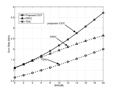
Figure 3: Sum rates versus SNRs for all RUEs with different schemes.

To evaluate performance gains of the agent, the data rates of the MUE versus SNRs are compared among the CICF, FRPC and TDIC in Fig. 4. It can be observed that the proposed CICF achieves the equivalent data rate for the MUE as the FRPC, which is not unexpected since the equality of the IR constraint would always hold when the BBU pool can acquire the complete and perfect CSI. Comparing with the baseline TDIC, the data-rate based utility gain for the MUE is significant for the proposed CICF because only partial spectral resources are utilized in the TDIC.

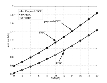
Figure 4: Data rates versus SNRs for MUEs with different schemes.

Summarizing the sum rates of all RUEs and MUE in Fig. 3 and Fig. 4, respectively, the rate-based utility gain from the proposed CICF is significant, which demonstrating the effectiveness of the proposed contract-based solution under perfect CSI.

V-B Performance Evaluations under Partial CSI

In Fig. 5, the sum rates of all RUEs versus SNRs under imperfect CSI for the proposed CICF and baselines (i.e., FRPC and TDIC) are evaluated and compared. Similarly to the results under perfect CSI, the proposed CICF can achieve a significant sum rate gain compared with the baselines due to the fact that both the time durations of the three phases and the allocated power are optimized. Moreover, comparing the performance gain gap from the CICF to FRPC in Fig. 3 and Fig. 5, the benefit of the principal under imperfect CSI is lower than that under perfect CSI. This happens because the derived optimal contract under imperfect CSI cannot always ensure the equality of all IR constraints. Furthermore, the performances of FRPC and TDIC under perfect CSI is better than that under imperfect CSI due to the fact that the channel estimation error degrades the precoding performance at RRHs.

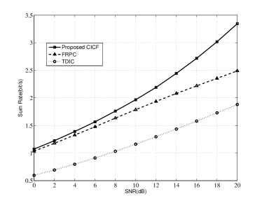
Figure 5: Sum rates versus SNRs for RUEs with different schemes.

In Fig. 6, data rates of the MUE versus SNRs under imperfect CSI are compared among the CICF, FRPC and TDIC. Comparing with FRPC, the agent can achieve a significant performance gain in the proposed CICF because the optimal contract under imperfect CSI cannot ensure the equality of all IR constraints. Meanwhile, the performance of FRPC in Fig. 6 is worse than that in Fig. 4 because the fairness power control depends critically on the instantaneous CSI. While TDIC in Fig. 6 is the same as that in Fig. 4 since the CSI has no impact on the downlink transmission of the MBS with this baseline.

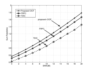
Figure 6: Data rates versus SNRs for MUEs with different schemes.

To characterize the optimal contract in the proposed CICF, the cumulative density function (cdf) of both $t_{1}^{*}$ and $t_{2}^{*}$ are plotted in Fig. 7. It can be seen that $P\!\left(t_{1}^{*}\!\geq\!0.5T_{0}\right)\!>\!0.7$ and $P\!\left(t_{2}^{*}\!\leq\!0.5T_{0}\right)\!>\!0.8$, which indicates that the time duration of Phase I should be longer than that of Phase II to optimize the sum date rates. To optimize the transmission data rates of the whole H-CRAN, more time resources should be assigned to allow MUEs to be served by RRHs, and thus an example of the transmission frame structure under these scheduling algorithms and configurations in this paper is suggested such that the time duration of Phase I is about 70 percent of the TTI length, and the time duration of Phase II is about 30 percent of the TTI length. Note that the transmission duration of Phase III would be zero when the contract is signed, which is indicated in both Lemma 1 and Lemma 2.

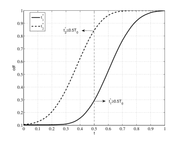
Figure 7: The cdf distributions of $t_{1}^{*}$ and $t_{2}^{*}$.

VI Conclusions

In this paper, a contract-based interference coordination framework has been proposed to mitigate inter-tier interference in H-CRANs, whose core idea is that the BBU pool is selected as the principal that would present a contract to the MBS, and the MBS as the agent decides whether to accept the contract or not according to its potential for improving the SE performance. An optimal contract design that maximizes the overall rate-based utility has been derived when perfect CSI is available at both principal and agent. Furthermore, the contract optimization under the situation where the partial CSI has been obtained from channel estimation has been considered as well. Monte Carlo simulations have been provided to corroborate the analysis, and simulation results have shown that the proposed framework can significantly increase the sum data rates, thus demonstrating the effectiveness of the proposed contract-based framework. Interesting topics for further research include, more advanced inter-tier interference coordination schemes to enhance the RRH-MBS with UEs-separated phase in the presented framework, and the inclusion of fronthaul constraints within this framework.

Appendix A Proof of Lemma 1

For the fixed $t_{1}$ and $t_{2}$, the optimal $P_{C1}$ and $P_{M1}$ can be derived by using the Karush-Kuhn-Tucker (KKT) conditions. The corresponding Lagrangian function can be written as

$$L (P_{C1},P_{M1},\lambda)\!=\!-t_{1}R_{C1}$$

$$\!-\!\lambda\left[P_{\mathrm{max}}\!-\!\frac{P_{C1}}{(K\!-\!M\!-\!1)\varepsilon_{1}}\!-\!\frac{P_{M1}}{(K\!-\!M\!-\!1)\upsilon_{M\!+\!1}}\right],$$ (64)

whose solution is derived as

$$\nabla L(P_{C1},P_{M1},\lambda)\!=-t_{1}\frac{\partial R_{C1}}{\partial P_{C1}}\!+\!\lambda\frac{1}{(K\!-\!M\!-\!1)\varepsilon_{1}}\!=\!0,$$ (65)

$$\lambda\left[P_{\rm{max}}\!-\!\frac{P_{C1}}{(K\!-\!M\!-\!1)\varepsilon_{1}}\!-\!\frac{P_{M1}}{(K\!-\!M\!-\!1)\upsilon_{M\!+\!1}}\right]=0,$$ (66)

$$\lambda\geq 0.$$ (67)

It is obvious that $\lambda$ must be positive to achieve the optimal solution for $P_{C1}$, and thus the optimal received powers $P_{C1}^{*}$ and $P_{M1}^{*}$ allocated to RUEs and MUE should satisfy

$$\frac{P_{C1}^{*}}{(K\!-\!M\!-\!1)\varepsilon_{1}}\!+\!\frac{P_{M1}^{*}}{(K\!-\!M\!-\!1)\upsilon_{M\!+\!1}}\!=\!P_{\mathrm{max}}.$$ (68)

For given $P_{C1}$ and $P_{M1}$, the optimal $t_{1}$ and $t_{2}$ can be obtained by solving following equations:

$$R_{C2}\!-\!R_{C1}\!+\!v\!-\!v_{1}\!-\!wR_{M1}\!=\!0,$$ (69)

$$R_{C2}\!-\!R_{C3}\!+\!v\!-\!v_{2}\!-\!wR_{M3}\!=\!0,$$ (70)

$$v_{1}t_{1}\!=\!0,\thinspace v_{2}t_{2}\!=\!0,\thinspace v(T\!-\!t_{1}\!-\!t_{2})\!=\!0,$$ (71)

$$\varpi(t_{1}R_{M1}\!+\!t_{3}R_{M3}\!-\!u)\!=\!0,$$ (72)

$$v_{1}\!\geq\!0,\thinspace v_{2}\!\geq\!0,\thinspace v\!\geq\!0,\thinspace\varpi\!\geq\!0.$$ (73)

where $v$, $\varpi$, $v_{1}$, and $v_{2}$ are the Lagrangian multipliers. It is obvious that $\varpi$ must be larger than zero. Therefore, the IR constraint is derived. Moreover, in order to maximize the transmission bit rate of the MUE, the optimal $t_{3}$ should be equal to zero.

Appendix B Proof of Lemma 2

Denoting the $m$-th column of $\mathbf{G}^{T}$ and $\mathbf{A}$ by $\mathbf{g}_{m}$ and $\mathbf{a}_{m}$, respectively, the transmission data rate can be derived as [32]

$$\hat{R}_{m}\!=\!$$

$$\log\!\left(1\!+\!\frac{|\mathcal{E}[\mathbf{g}_{m}\mathbf{a}_{m}]|^{2}}{\sigma_{n}^{2}\!+\!\textup{var}\{\mathbf{g}_{m}\mathbf{a}_{m}\}\!+\!|f_{Bm}|^{2}P_{B}\!+\!\sum_{i\neq m}^{M}\mathcal{E}[|\mathbf{g}_{m}\mathbf{a}_{i}|^{2}]}\right).$$ (74)

For the ZF precoder, we have $\mathbf{\hat{g}}_{m}\mathbf{a}_{i}\!=\!\delta_{mi}$. Denote the radio channel matrix by $\mathcal{G}\!=\!\hat{\mathbf{G}}\!+\!\tilde{\mathbf{G}}$, where $\tilde{\mathbf{G}}$ is the estimation error, and we have

$$\mathbf{g}_{m}\mathbf{a}_{i}\!=\!\hat{\mathbf{g}}_{m}\mathbf{a}_{i}+\!\tilde{\mathbf{g}}_{m}\mathbf{a}_{i}=\!\delta_{mi}\!+\!\tilde{\mathbf{g}}_{m}\mathbf{a}_{i}.$$ (75)

According to (75), the expectation and variance can be written as

$$\mathcal{E}[\mathbf{g}_{m}\mathbf{a}_{i}]\! =\!P_{C1},\thinspace\mathcal{E}[|\mathbf{g}_{m}\mathbf{a}_{i}|^{2}]\!=\!\delta_{1}P_{C1}\sum_{i\neq m}^{M}\left[\mathbf{G}\mathbf{G}^{H}\right]^{-1}_{ii},$$ (76)

$$\textup{var}\{\mathbf{g}_{m}\mathbf{a}_{i}\}\! =\!\mathcal{E}\left[\mathbf{a}_{m}^{H}\mathbf{g}_{m}^{H}\mathbf{g}_{m}\mathbf{a}_{m}\right]\!=\!\delta_{1}P_{C1}\left[\mathbf{G}\mathbf{G}^{H}\right]^{-1}_{mm}.$$ (77)

Thus, the sum data rate of all RUEs in the downlink transmission during Phase III is given by

$$\hat{R}_{C3}\!=\!\sum_{m\!=\!1}^{M}\!\log\!\!\left(1\!+\!\frac{P_{C3}}{\delta_{1}P_{C3}\mathrm{tr}\!\bigg{\{}\left[\hat{\mathbf{G}}\hat{\mathbf{G}}^{H}\right]^{-1}\bigg{\}}\!+\!|f_{Bm}|^{2}P_{B}\!+\!\sigma_{n}^{2}}\right),$$ (78)

and the data rate of the MUE can be written as

$$\hat{R}_{M3}\! =\!\log\left(1\!+\!\frac{|g_{B}|^{2}P_{B}}{\sigma_{n}^{2}\!+\!|\mathbf{fA}|^{2}}\right)$$

$$=\!\log\left(1\!+\!\frac{|g_{B}|^{2}P_{B}}{P_{C3}\mathbf{f}\hat{\mathbf{G}}^{H}\left(\hat{\mathbf{G}}\hat{\mathbf{G}}^{H}\right)^{-2}\hat{\mathbf{G}}\mathbf{f}^{H}\!+\!\sigma_{n}^{2}}\right).$$ (79)

Similarly, the sum rates during the Phase I and II can be calculated in the same way.

Appendix C Proof of Lemma 3

By using the KKT conditions, the optimal $\tilde{t}_{3}^{L}$ can be obtained by solving the following equations:

$$-(\tilde{R}_{C2}\!-\!\tilde{R}_{C1})q_{L}\frac{\tilde{R}_{M3}^{L}}{\tilde{R}_{M1}}$$

$$\quad\quad\!+\!(\tilde{R}_{C2}\!-\!\tilde{R}_{C3})q_{L}\!-\!\omega_{1}\!+\!\omega_{2}(1\!-\!\frac{\tilde{R}_{M3}^{L}}{\tilde{R}_{M1}})=0,$$ (80)

$$\omega_{1}t_{3}^{L}\!=\!0,\thinspace\omega_{2}(T_{0}\!-\!\tilde{t}_{1}^{L}\!-\!t_{3}^{L})\!=\!0,$$ (81)

$$\omega_{1}\!\geq\!0,\thinspace\omega_{2}\!\geq\!0.$$ (82)

Based on (80), (81), and (82), we have the following results:

• When $\tilde{R}_{M1}(\tilde{R}_{C2}-\tilde{R}_{C3})\!>\!\tilde{R}_{M3}^{L}(\tilde{R}_{C2}\!-\!\tilde{R}_{C1})$, $\omega_{1}$ must be positive, i.e., $t_{3}^{L}\!=\!0$. As $t_{3}^{l}$ ($l=1,\ldots,L-1$) is often less than $t_{3}^{L}$, $t_{3}^{l}$ is equal to zero.

• When $\tilde{R}_{M1}(\tilde{R}_{C2}-\tilde{R}_{C3})\!=\!\tilde{R}_{M3}^{L}(\tilde{R}_{C2}\!-\!\tilde{R}_{C1})$, $t_{3}^{L}$ can be an arbitrary value in the interval $[0,T_{0}]$. The derivative of $-U_{C}^{*}$ with respect to $t_{3}^{L\!-\!1}$ can be written as

  $$(\tilde{R}_{C2}\!-\!\tilde{R}_{C1})\left[q_{L}\!+\!q_{L\!-\!1}\right](\tilde{R}_{M3}^{L}-\tilde{R}_{M3}^{L-1})>0.$$ (83)

  To maximize $U_{C}^{*}$, we have $t_{3}^{L\!-\!1}\!=\!0$, and all $t_{3}^{l}$ ($l<L-1$) should be equal to zero.

• When $\tilde{R}_{M1}(\tilde{R}_{C2}-\tilde{R}_{C3})\!<\!\tilde{R}_{M3}^{L}(\tilde{R}_{C2}\!-\!\tilde{R}_{C1})$, $\omega_{2}$ must be positive. Meanwhile, the following equation holds:

  $$T_{0}\!=\!\tilde{t}_{1}^{L}\!+\!t_{3}^{L}.$$ (84)

  Obviously, this contract is unacceptable for the agent. Therefore, $t_{3}^{L}$ should be equal to $T_{0}$. In order to satisfy the IR constraint, $t_{3}^{l}$ ($l=1,\ldots,L-1$) should be set as zero.

As for the optimal powers assigned to RRHs and MBS in Phase I, when $t_{3}^{l}$ $(l=1,\ldots,L-1)$ is equal to zero, $U_{C}^{*}$ can be expressed as

$$U_{C}^{*}\!=\!\frac{(\tilde{R}_{C1}\!-\!\tilde{R}_{C2})u_{L}}{\tilde{R}_{M1}}\!+\!T_{0}(\tilde{R}_{C3}\!-\!\tilde{R}_{C2}).$$ (85)

The Lagrangian function can be written as

$$L_{1} (P_{C1},P_{M1},\lambda_{1})\!=\!-\underbrace{\frac{(\tilde{R}_{C1}\!-\!\tilde{R}_{C2})u_{L}}{\tilde{R}_{M1}}}_{f_{1}(P_{C1},P_{M1})}$$

$$\!-\!\lambda_{1}\left[P_{\mathrm{max}}\!-\!\frac{P_{C1}}{(K\!-\!M\!-\!1)\varepsilon_{2}}\!-\!\frac{P_{M1}}{(K\!-\!M\!-\!1)(\upsilon_{M\!+\!1}+\delta_{2})}\right].$$ (86)

The derivative of the Lagrangian function with respect to $P_{C1}$ is

$$\nabla L_{1}(P_{C1},P_{M1},\lambda_{1})\!=$$

$$\quad\quad-\frac{\partial f_{1}(P_{C1},P_{M1})}{\partial P_{C1}}\!+\!\lambda_{1}\frac{1}{(K\!-\!M\!-\!1)\varepsilon_{2}}\!=\!0,$$ (87)

$$\lambda_{1}\left[P_{max}\!-\!\frac{P_{C1}}{(K\!-\!M\!-\!1)\varepsilon_{2}}\!-\!\frac{P_{M1}}{(K\!-\!M\!-\!1)(\upsilon_{M\!+\!1}+\delta_{2})}\right]=0.$$ (88)

$$\lambda_{1}\geq 0.$$ (89)

Since the derivative of $f_{1}(P_{C1},P_{M1})$ with respect to $P_{C1}$ is positive, $\lambda^{*}$ must be positive, and the optimal powers $P_{C1}^{*}$ and $P_{M1}^{*}$ should satisfy

$$\frac{P_{C1}^{*}}{(K\!-\!M\!-\!1)\varepsilon_{2}}\!+\!\frac{P_{M1}^{*}}{(K\!-\!M\!-\!1)(\upsilon_{M\!+\!1}\!+\!\delta_{2})}\!=\!P_{\mathrm{max}}.$$ (90)

If $t_{3}^{L}$ is positive, $U_{C}^{*}$ can be re-written as

$$U_{C}^{*}\! =\!(\tilde{R}_{C1}\!-\!\tilde{R}_{C2})[1-q_{L}]\frac{u_{L}}{\tilde{R}_{M1}}\!$$

$$+\!(\tilde{R}_{C1}\!-\!\tilde{R}_{C2})q_{L}\frac{u_{L}\!-\!\tilde{R}_{M3}^{L}}{\tilde{R}_{M1}}+\!T_{0}(\tilde{R}_{C3}\!-\!\tilde{R}_{C2})[1-q_{L}].$$ (91)

Similarly, the Lagrangian function is re-formulated as

$$L_{2}(P_{C1},P_{M1},\lambda_{2})\!=\!$$

$$-\underbrace{(\tilde{R}_{C1}\!-\!\tilde{R}_{C2})[1-q_{L}]\frac{u_{L}}{\tilde{R}_{M1}}\!+\!(\tilde{R}_{C1}\!-\!\tilde{R}_{C2})q_{L}\frac{u_{L}\!-\!\tilde{R}_{M3}^{L}}{\tilde{R}_{M1}}}_{f_{2}(P_{C1},P_{M1})}\!$$ (92)

$$-\!\lambda_{2}\left[P_{\mathrm{max}}\!-\!\frac{P_{C1}}{(K\!-\!M\!-\!1)\varepsilon_{2}}\!-\!\frac{P_{M1}}{(K\!-\!M\!-\!1)(\upsilon_{M\!+\!1}+\delta_{2})}\right].$$ (93)

As the derivative of $f_{2}(P_{C1},P_{M1})$ with respect to $P_{C1}$ is also positive, the optimal powers allocated to $P_{C1}^{*}$ and $P_{M1}^{*}$ are the same as in (90).

Mugen Peng (M’05–SM’11) received the B.E. degree in Electronics Engineering from Nanjing University of Posts & Telecommunications, China in 2000 and a PhD degree in Communication and Information System from the Beijing University of Posts & Telecommunications (BUPT), China in 2005. After the PhD graduation, he joined in BUPT, and has become a full professor with the school of information and communication engineering in BUPT since Oct. 2012. During 2014, he is also an academic visiting fellow in Princeton University, USA. He is leading a research group focusing on wireless transmission and networking technologies in the Key Laboratory of Universal Wireless Communications (Ministry of Education) at BUPT. His main research areas include wireless communication theory, radio signal processing and convex optimizations, with particular interests in cooperative communication, radio network coding, self-organizing network, heterogeneous network, and cloud communication. He has authored/coauthored over 50 refereed IEEE journal papers and over 200 conference proceeding papers. Dr. Peng is currently on the Editorial/Associate Editorial Board of the IEEE Communications Magazine, the IEEE Access, the IET Communications, the International Journal of Antennas and Propagation (IJAP), the China Communications, and the International Journal of Communications System (IJCS). He has been the guest leading editor for the special issues in the IEEE Wireless Communications. Dr. Peng was a recipient of the 2014 IEEE ComSoc AP Outstanding Young Researcher Award, and the best paper award in GameNets 2014, CIT 2014, ICCTA 2011, IC-BNMT 2010, and IET CCWMC 2009. He received the First Grade Award of Technological Invention Award in Ministry of Education of China for his excellent research work on the hierarchical cooperative communication theory and technologies, and the Second Grade Award of Scientific and Technical Advancement from China Institute of Communications for his excellent research work on the co-existence of multi-radio access networks and the 3G spectrum management.

Xinqian Xie received the B.S. degree in telecommunication engineering from the Beijing University of Posts and Communications (BUPT), China, in 2010. He is currently pursuing the Ph.D. degree at BUPT. His research interests include cooperative communications, estimation and detection theory.

Qiang Hu received the B.S. degree in applied physics from the Beijing University of Posts & Communications (BUPT), China, in 2013. He is currently pursuing the Master degree at BUPT. His research interests include cooperative communications, such as cloud radio access networks (C-RANs), and statistical signal processing in large-scale networks.

Jie Zhang (M’02) is a full professor and has held the Chair in Wireless Systems at the Electronic and Electrical Engineering Dept., University of Sheffield since 2011. He received PhD in 1995 and became a Lecturer, Reader and Professor in 2002, 2005 and 2006 respectively. He and his students pioneered research in femto/small cell and HetNets and published some of the most widely cited publications in these topics. He co-founded RANPLAN Wireless Network Design Ltd. (www.ranplan.co.uk) that produces a suite of world leading in-building distributed antenna system, indoor-outdoor small cell/HetNet network design and optimization tools “iBuildNet-Professional, Tablet and Cloud”. Since 2003, he has been awarded over 20 projects by the EPSRC, the EC FP6/FP7/H2020 and industry, including some of earliest research projects on femtocell/HetNets.

H. Vincent Poor (S’72, M’77, SM’82, F’87) received the Ph.D. degree in EECS from Princeton University in 1977. From 1977 until 1990, he was on the faculty of the University of Illinois at Urbana-Champaign. Since 1990 he has been on the faculty at Princeton, where he is the Michael Henry Strater University Professor of Electrical Engineering and Dean of the School of Engineering and Applied Science. Dr. Poor’s research interests are in the areas of information theory, statistical signal processing and stochastic analysis, and their applications in wireless networks and related fields including social networks and smart grid. Among his publications in these areas are the recent books Principles of Cognitive Radio (Cambridge University Press, 2013) and Mechanisms and Games for Dynamic Spectrum Allocation (Cambridge University Press, 2014). Dr. Poor is a member of the National Academy of Engineering, the National Academy of Sciences, and is a foreign member of Academia Europaea and the Royal Society. He is also a fellow of the American Academy of Arts and Sciences, the Royal Academy of Engineering (U. K), and the Royal Society of Edinburgh. He received the Marconi and Armstrong Awards of the IEEE Communications Society in 2007 and 2009, respectively. Recent recognition of his work includes the 2014 URSI Booker Gold Medal, and honorary doctorates from Aalborg University, Aalto University, the Hong Kong University of Science and Technology, and the University of Edinburgh.

References

- [1] M. Peng and W. Wang, “Technologies and standards for TD-SCDMA evolutions to IMT-Advanced,” IEEE Commun. Mag., vol. 47, no. 12, pp. 50–58, Dec. 2009.
- [2] M. Peng, Y. Liu, D. Wei, W. Wang, and H. Chen, “Hierarchical cooperative relay based heterogeneous networks,” IEEE Wireless Commun., vol. 18, no. 3, pp. 48–56, Jun. 2011.
- [3] M. Peng, D. Liang, Y. Wei, J. Li, and H. Chen, “Self-configuration and self-optimization in LTE-Advanced heterogeneous networks,” IEEE Commun. Mag., vol. 51, no. 5, pp. 36–45, May 2013.
- [4] W. Shin, W. Noh, K. Jang, and H. Choi, “Hierarchical interference alignment for downlink heterogeneous networks,” IEEE Trans. Wireless Commun., vol. 11, no. 12, pp. 4549–4559, Dec. 2012.
- [5] M. Peng, X. Zhang, and W. Wang, “Performance of orthogonal and co-channel resource assignments for femto-cells in LTE systems,” IET Communications, vol. 7, no. 5, pp. 996–1005, May 2011.
- [6] P. Xia, C. Liu, and J. G. Andrews, “Downlink coordinated multi-point with overhead modeling in heterogeneous cellular networks,” IEEE Trans. Wireless Commun., vol. 12, no. 8, pp. 4025–4037, Aug. 2013.
- [7] R. Irmer, H. Droste, P. Marsch et al., “Coordinated multipoint: Concepts, performance, and field trial results,” IEEE Commun. Mag., vol. 49, no. 2, pp. 102–111, Feb. 2011.
- [8] M. Peng, C. I, C. Tan, and C. Huang, “IEEE access special section editorial: Recent advances in cloud radio access networks,” IEEE Access, vol. 2, pp. 1683–1685, Dec. 2014.
- [9] X. Xie, M. Peng, W.Wang, and H. V. Poor, “Training design and channel estimation in uplink cloud radio access networks,” IEEE Signal Process. Letters, vol. 22, no. 8, pp. 1060–1064, Aug. 2015.
- [10] M. Peng, S. Yan, and H. V. Poor, “Ergodic capacity analysis of remote radio head associations in cloud radio access networks,” IEEE Wireless Commun. Letters, vol. 3, no. 4, pp. 365–368, Aug. 2014.
- [11] M. Peng, Y. Li, J. Jiang, J. Li, and C. Wang, “Heterogeneous cloud radio access networks: A new perspective for enhancing spectral and energy efficiencies,” IEEE Wireless Commun., vol. 21, no. 6, pp. 126–135, Dec. 2014
- [12] M. Peng, Y. Li, Z. Zhao, and C. Wang, “System architecture and key technologies for 5G heterogeneous cloud radio access networks,” to appear in IEEE Network.
- [13] D. Lopez-Perez, I. Guvenc, G. de la Roche et al., “Enhanced intercell interference coordination challenges in heterogeneous networks,” IEEE Wireless Commun., vol. 18, no. 3, pp. 22–30, Mar. 2011.
- [14] S. Zhang, S. Liew, and H. Wang “Blind known interference cancellation ,” IEEE J. Sel. Areas Commun., vol. 31, no. 8, pp. 1572–1582, Aug. 2013.
- [15] W. Cheung, T. Quek, and M. Kountouris, “Throughput optimization, spectrum allocation, and access control in two-tier femtocell networks,” IEEE J. Sel. Areas Commun., vol. 30, no. 3, pp. 561–574, Apr. 2012.
- [16] A. Liu and V. Lau, “Joint power and antenna selection optimization in large cloud radio access networks,” IEEE Trans. Signal Process., vol. 62, no. 5, pp. 1319-1328, Feb. 2014.
- [17] J. Wang, M. Peng, S. Jin, and C. Zhao, “A generalized Nash equilibrium approach for robust cognitive radio networks via generalized variational inequalities,” IEEE Trans. Wireless Commun., vol. 13, no. 7, pp. 3701–3714, Jul. 2014.
- [18] S. Guruacharya, D. Niyato, I. Dong, and E. Hossain, “Hierarchical competition for downlink power allocation in OFDMA femtocell networks,” IEEE Trans. Wireless Commun., vol. 12, no. 4, pp. 1543-1553, Apr. 2013.
- [19] X. Kang, R. Zhang, and M. Motani, “Price-based resource allocation for spectrum-sharing femtocell networks: A stackelberg game approach,” IEEE J. Sel. Areas Commun., vol. 30, no. 3, pp. 538–549, Apr. 2012.
- [20] Q. Han, Y. Bo, X. Wang, K. Ma, and C. Chen, “Hierarchical-Game-Based uplink power control in femtocell networks,” IEEE Trans. Veh. Technol., vol. 63, no. 6, pp. 2819–2835, Jul. 2014.
- [21] L. Duan, L. Gao, and J. Huang, “Cooperative spectrum sharing: a contract-based approach,” IEEE Trans. Mobile Comput., vol. 13, no. 1, pp. 174–187, Jan. 2014.
- [22] L. Gao, X. Wang, Y. Xu, and Q. Zhang, “Spectrum trading in cognitive radio networks: a contract-theoretic modeling approach,” IEEE J. Sel. Areas Commun., vol. 29, no. 4, pp. 843–855, Apr. 2011.
- [23] Z. Hasan and V. Bhargava, “Relay selection for OFDM wireless systems under asymmetric information: a contract-theory based approach,” IEEE Trans. Wireless Commun., vol. 12, no. 8, pp. 3824–3837, Aug. 2013.
- [24] V. R. Cadambe and S. A. Jafar, “Interference alignment and degrees of freedom of the K-user interference channel,” IEEE Trans. Inf. Theory, vol. 54, no. 8, pp. 3425–3441, Aug. 2008.
- [25] M. Biguesh and A. B. Gershman,“Training-based MIMO channel estimation: a study of estimator tradeoffs and optimal training signals,” IEEE Trans. Signal Process., vol. 54, no. 3, pp. 884–893, Mar. 2006.
- [26] N. Lee, O. Simeone, and J. Kang, “The effect of imperfect channel knowledge on a MIMO system with interference, ” IEEE Trans. Commun., vol. 60, no. 8, pp. 2221–2229, Aug. 2012.
- [27] J. Choi and F. Adachi, “User selection criteria for multiuser systems with optimal and suboptimal LR based detectors,” IEEE Trans. Signal Process., vol. 58, no. 10, pp. 5463–5468, Oct. 2010.
- [28] R. Rogolin, O. Y. Bursalioglu, H. Papadopoulos, G. Caire et al., “Scalable synchronization and reciprocity calibration for distributed multiuser MIMO,” IEEE Trans. Wireless Commun., vol. 13, no. 4, Apr. 2014.
- [29] M. Sichitiu and C. Veerarittiphan, “Simple, accurate time synchronization for wireless sensor networks,” in Proc. IEEE Wireless Communications and Networking Conference (WCNC), New Orleans, LA, Mar. 2003, pp. 1266–1273.
- [30] Y. Jing and S. ShahbazPanahi, “Max-min optimal joint power control and distributed beamforming for two-way relay networks under per-node power constraints,” IEEE Trans. Signal Process., vol. 60, no. 12, pp. 6576–6589, Dec. 2012.
- [31] B.Patrick and M. Dewatripont, Contract Theory, MIT Press, 2005.
- [32] J. Jose, A. Ashikhmin, T. L. Marzetta, and S. Vishwanath, “Pilot contamination and precoding in multi-cell TDD systems, ” IEEE Trans. Wireless Commun., vol. 10, no. 8, pp. 2640–2650, Aug. 2011.