A multi-dimensional, energy- and charge-conserving, nonlinearly implicit, electromagnetic Vlasov-Darwin particle-in-cell algorithm

Abstract

For decades, the Vlasov-Darwin model has been recognized to be attractive for particle-in-cell (PIC) kinetic plasma simulations in non-radiative electromagnetic regimes, to avoid radiative noise issues and gain computational efficiency. However, the Darwin model results in an elliptic set of field equations that renders conventional explicit time integration unconditionally unstable. Here, we explore a fully implicit PIC algorithm for the Vlasov-Darwin model in multiple dimensions, which overcomes many difficulties of traditional semi-implicit Darwin PIC algorithms. The finite-difference scheme for Darwin field equations and particle equations of motion is space-time-centered, employing particle sub-cycling and orbit-averaging. The algorithm conserves total energy, local charge, canonical-momentum in the ignorable direction, and preserves the Coulomb gauge exactly. An asymptotically well-posed fluid preconditioner allows efficient use of large time steps and cell sizes, which are determined by accuracy considerations, not stability, and can be orders of magnitude larger than required in a standard explicit electromagnetic PIC simulation. We demonstrate the accuracy and efficiency properties of the algorithm with various numerical experiments in 2D-3V.

1 Introduction

The electromagnetic (EM) Particle-in-cell (PIC) method solves Vlasov-Maxwell’s equations for kinetic plasma simulations [1, 2]. In the standard approach, Maxwell’s equations are solved on a grid, and the Vlasov equation is solved by the method of characteristics using a large number of particles, from which the evolution of the probability distribution function (PDF) is obtained. The field-PDF description is tightly coupled. Maxwell’s equations (or a subset thereof) is driven by moments of the PDF such as charge density and/or current density. The PDF, on the other hand, follows a hyperbolic equation in phase space, whose characteristics are determined by the fields self-consistently.

Here, we are interested in the Vlasov-Darwin approximation to the Vlasov-Maxwell set of equations, useful for low-frequency plasma applications in so-called non-radiative regimes. The Darwin model of electrodynamics, which is $O(v/c)^{2}$ approximation of the Maxwell’s equations [3], eliminates the light-wave propagation in the plasma. In doing so, the Darwin model avoids unwanted electromagnetic wave excitation and related instabilities [4, 5, 6]. However, the Vlasov-Darwin equations turn out to be more difficult to solve in practice than Vlasov-Maxwell, despite the fact that Darwin equations are seemingly simpler (without the 2nd-order time derivative of vector potential, or the transverse displacement current). Mathematically, this simplification fundamentally changes the character of the field equations from hyperbolic to elliptic. As a consequence, explicit time integration schemes (commonly used for Vlasov-Maxwell PIC algorithms) are unconditionally unstable [7]. To overcome the difficulty, semi-implicit moment methods have been proposed [7] (and have become the standard, see Refs. [8, 9, 10, 11, 12, 13, 14, 15, 16, 17] and references therein) to time-advance the Vlasov-Darwin PIC system. However, the semi-implicit moment method is notably more complicated and difficult to solve than explicit schemes for the Vlasov-Maxwell equations, especially with non-periodic boundary conditions [18, 19, 10, 12].

Fully nonlinearly implicit PIC algorithms [20, 6, 21, 22] take advantage of modern iterative solvers, e.g. Jacobian-free Newton-Krylov (JFNK) methods [23] to converge the field-particle system nonlinearly. A tight nonlinear tolerance is enforced for convergence between particles, moments, and self-consistent fields at each timestep. Moment equations can be effectively used in the preconditioner stage of JFNK [24, 22], to accelerate the convergence of the iterative kinetic solver. Discrete conservation theorems for total energy, local charge, and particle canonical momentum can be derived for those algorithms, which are attractive for long-time simulations. Particle orbit integration is subcycled [20, 22], resulting in much improved orbit accuracy, and allowing an efficient implementation on modern computer architectures [25]. As a consequence, these algorithms have shown the ability to overcome many difficulties of traditional semi-implicit PIC algorithms (e.g., implicit-moment [26, 27, 28, 29, 30, 31], direct-implicit methods [32, 33, 34, 35, 36], and Darwin implementations [7, 8, 10, 11]) for accurate long-term kinetic simulations.

The main objective of this study is to generalize the 1D-3V study in Ref. [22] to deliver an implicit, conservative Darwin-PIC algorithm in multiple dimensions. The algorithm employs the potential ($\phi$-$\mathbf{A}$) formulation of the Darwin equations. Both field and particle equations are discretized using a space-time-centered finite difference scheme. As in 1D [22], the fully implicit character of the implementation is key to realize the desired conservation and performance properties. Particles are substepped for orbit integration accuracy, as particle time scales may be much faster than field time scales. Synchronization between fields and particles is accomplished by orbit-averaging [20]. We prove conservation theorems for global energy, local charge, particle canonical momentum, and the preservation of the Coulomb gauge ($\nabla\cdot\mathbf{A}=0$) on a uniform grid in a periodic plasma system. A moment-based preconditioner is formulated by taking the zeroth and first moment of the Vlasov equation. Fluid and ambipolar asymptotic regimes are handled effectively by the fluid preconditioner. The performance of the preconditioner is, however, limited by electron Bernstein modes, which are not captured by the simplified moment system employed. As a result, the kinetic solver is robust against variations in domain sizes as well as mass ratios, provided that electron Bernstein mode timescales are respected. In practice, for a given magnetization, this sets a lower limit for the electron-ion mass ratio.

The rest of the paper is organized as follows. Section 2 introduces our formulation for the general Vlasov-Darwin model and its favorable properties. The model is specified in 2D-3V and discretized with an implicit central-difference scheme in Sec. 3, where we propose a new automatic charge-conserving particle-moving scheme for multiple dimensions, and prove theorems for the exact conservation of global energy and particle canonical momenta in a discrete setting, as well as the preservation of the Coulomb gauge. Section 4 provides a detailed description of moment-based preconditioning for the JFNK kinetic solver. Numerical examples demonstrating the accuracy, performance, and conservation properties of the algorithm are presented in Sec. 5. Finally, we conclude in Sec. 6.

2 Electromagnetic Vlasov-Darwin model

The Vlasov-Darwin equations for a collisionless electromagnetic plasma can be written as [7, 37, 19, 38, 39, 22]:

$$\partial_{t}f_{\alpha}+\mathbf{v}\cdot\nabla f_{\alpha}+\frac{q_{\alpha}}{m_{\alpha}}(\mathbf{E}+\mathbf{v}\times\mathbf{B})\cdot\nabla_{v}f_{\alpha} = 0,$$ (1)

$$\frac{1}{\mu_{0}}\nabla^{2}\mathbf{A}+\mathbf{j}-\epsilon_{0}\partial_{t}\nabla\phi = 0,$$ (2)

$$\epsilon_{0}\nabla^{2}\phi+\rho = 0,$$ (3)

where $f_{\alpha}(\mathbf{r},\mathbf{v})$ is the particle distribution function of species $\alpha$ in phase space, $q_{\alpha}$ and $m_{\alpha}$ are the species charge and mass respectively, $\epsilon_{0}$ and $\mu_{0}$ are the vacuum permittivity and permeability respectively, $\phi$ and $\mathbf{A}$ are the t scalar and vector potentials, respectively. The electric and magnetic fields are defined uniquely from $\phi,$ $\mathbf{A}$ as:

$$\mathbf{E}=-\nabla\phi-\partial_{t}\mathbf{A}\,\,;\,\,\mathbf{B}=\nabla\times\mathbf{A}.$$ (4)

The set of Darwin equations is driven by the plasma current density

$$\mathbf{j}=\sum_{\alpha}q_{\alpha}\int f_{\alpha}\mathbf{v}d\mathbf{v}.$$ (5)

Unlike Maxwell’s equations, the Darwin model does not feature Gauge invariance, and only the Coulomb gauge

$$\nabla\cdot\mathbf{A}=0$$ (6)

is physically acceptable (to enforce charge conservation).

Note that the Vlasov-Darwin model (Eqs. 1-6) is overdetermined, as it has more equations than unknowns. It features two involutions [40, 41]: Poisson’s equation and the solenoidal constraint of the vector potential. (An involution is a constraint satisfied by the solution of the system at all times, if satisfied initially.) These two involutions are not redundant, and must be enforced numerically [1, p. 359] to prevent spurious modes from being excited [42].

To solve the above Vlasov-Darwin equations, we begin by realizing that the two involutions do not need to be enforced explicitly. In stead of Poisson’s equation, we consider the equation:

$$\epsilon_{0}\partial_{t}\nabla^{2}\phi-\nabla\cdot\mathbf{j}=0,$$ (7)

found by taking the divergence of Eq. 2 and using Eq. 6. The two involutions are then implied by Eqs. 1, 2 and 7 when the local charge conservation equation,

$$\partial_{t}\rho+\nabla\cdot\mathbf{j}=0,$$ (8)

(which is implied independently by the Vlasov equation, Eq. 1) is satisfied. In particular, Poisson’s equation is implied by Eq. 3 and Eq. 8. The solenoidal constraint is implied as well, as can be seen by taking the divergence of Eq. 2 and using Eq. 3, to find:

$$\nabla\cdot\nabla^{2}\mathbf{A}=0,$$

from which, with appropriate conditions, Eq. 6 follows [42]. The derivation requires that $\nabla\cdot(\nabla^{2}\mathbf{A})=\nabla^{2}(\nabla\cdot\mathbf{A})=0$, and the boundary conditions be consistent with $\nabla\cdot\mathbf{A}=0$ at the boundary [43] (i.e., they must enforce continuity of the normal component of the vector potential at the boundary).

Equations 1, 2, 4, 5, and 7 constitute the minimal Vlasov-Darwin equation set of choice in this study. We emphasize that the main advantage of this set is that the two involutions (Poisson’s equation and the solenoidal constraint of $\mathbf{A}$) are built-in, and thus do not need to be enforced or solved explicitly when local charge is strictly conserved. This property, when implemented discretely, will be most advantageous for both accuracy (it avoids spurious modes) and efficiency (it avoids the extra divergence-cleaning step via conventional projection methods [44] or hyperbolic cleaning [45]). Most importantly, this formulation avoids explicitly enforcing Eq. 6, which has been a critical implementation roadblock for the Darwin approximation in multiple dimensions in previous studies [7, 10]. Carrying the involution enforcement to the discrete will require a very careful discrete treatment, however, and in particular one that strictly conserves local charge.

3 Multi-dimensional, implicit, particle-based discretization of the Vlasov-Darwin model

We employ a centered finite difference method to discretize the 2D-3V Vlasov-Darwin equations in Cartesian geometry on a uniform Yee grid (see Fig. 1), which has $N_{x}$ and $N_{y}$ cells in the $x$ and $y$ directions, respectively. The field equations (Eq. 2, 3) are written by replacing the derivatives with central difference schemes at the $n+\nicefrac{{1}}{{2}}$ time level as

$$\frac{1}{\mu_{0}}(\delta_{x}^{2}+\delta_{y}^{2})\left(\begin{array}[]{c}[A_{x}]_{i+\nicefrac{{1}}{{2}},j}\\ {}[A_{y}]_{i,j+\nicefrac{{1}}{{2}}}\\ {}[A_{z}]_{i,j}\end{array}\right)^{n+\nicefrac{{1}}{{2}}}+\left(\begin{array}[]{c}[\bar{j}_{x}]_{i+\nicefrac{{1}}{{2}},j}\\ {}[\bar{j}_{y}]_{i,j+\nicefrac{{1}}{{2}}}\\ {}[\bar{j}_{z}]_{i,j}\end{array}\right)^{n+\nicefrac{{1}}{{2}}}-\epsilon_{0}\delta_{t}\left(\begin{array}[]{c}\delta_{x}[\phi]_{i+\nicefrac{{1}}{{2}},j}\\ \delta_{y}[\phi]_{i,j+\nicefrac{{1}}{{2}}}\\ 0\end{array}\right)^{n+\nicefrac{{1}}{{2}}} = 0,$$ (18)

$$\epsilon_{0}\delta_{t}(\delta_{x}^{2}+\delta_{y}^{2})[\phi]_{i,j}^{n+\nicefrac{{1}}{{2}}}-\left(\delta_{x}[\bar{j}_{x}]_{i,j}+\delta_{y}[\bar{j}_{y}]_{i,j}\right)^{n+\nicefrac{{1}}{{2}}} = 0,$$ (19)

where the subscripts $i$ and $j$ denote cell index in the $x$ and $y$ directions, respectively, and $1\leq i\leq N_{x}$, $1\leq j\leq N_{y}$. The orbit-averaged current density $\bar{\mathbf{j}}$ is found from particles as described below. We define $Q^{n+\nicefrac{{1}}{{2}}}=(Q^{n+1}+Q^{n})/2$, where $Q$ is one of the unknown quantities. The finite-difference operation in time is defined at $n+\nicefrac{{1}}{{2}}$ as $\delta_{t}[Q]\equiv(Q^{n+1}-Q^{n})/\Delta t$. The first-order derivative in space is defined at the center of the two adjacent values, e.g., $\delta_{x}[\phi]_{i+\nicefrac{{1}}{{2}},j}=(\phi_{i+1,j}-\phi_{i,j})/\Delta x$. The second-order derivative in space is defined at the center of two adjacent first-order derivatives, e.g., $\delta_{x}^{2}[\phi]_{i,j}=(\delta_{x}[\phi]_{i+\nicefrac{{1}}{{2}},j}-\delta_{x}[\phi]_{i-\nicefrac{{1}}{{2}},j})/\Delta x$. Similar definitions are set for quantities at cell faces, e.g., $\delta_{x}[j_{x}]_{i,j}=(j_{i+\nicefrac{{1}}{{2}},j}-j_{i-\nicefrac{{1}}{{2}},j})/\Delta x$, and $(\delta_{x}^{2}+\delta_{y}^{2})[A_{x}]_{i+\nicefrac{{1}}{{2}},j}\equiv(A_{xi+\nicefrac{{3}}{{2}},j}-2A_{xi+\nicefrac{{1}}{{2}},j}+A_{xi-\nicefrac{{1}}{{2}},j})/\Delta x^{2}+(A_{xi+\nicefrac{{1}}{{2}},j+1}-2A_{xi+\nicefrac{{1}}{{2}},j}+A_{xi+\nicefrac{{1}}{{2}},j-1})/\Delta y^{2}$, etc.

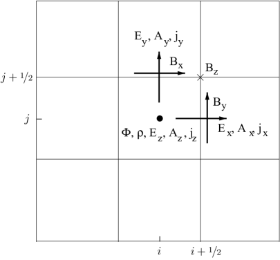
Figure 1: 2D Yee grid and associated quantities. An integer index $i$ or $j$ denotes a cell center, and a half index $i+\nicefrac{{1}}{{2}}$ or $j+\nicefrac{{1}}{{2}}$ denotes a cell face.

The current density $\bar{\mathbf{j}}$ in Eqs 18, 19 is gathered from particles by orbit-averaging the individual current contributions,

$$\bar{\mathbf{j}}^{n+1/2}=\frac{1}{\Delta t}\sum_{p}\sum_{\nu=0}^{N_{\nu}-1}\mathbf{j}_{p}^{\nu+1/2}\Delta\tau_{p}^{\nu},$$ (20)

where the index $\nu$ denotes a substep, with subtimestep $\Delta\tau_{p}^{\nu}$, and $N_{\nu}$ denotes the number of substeps. Particle substeps satisfy $\sum_{\nu=0}^{N_{\nu}-1}\Delta\tau_{p}^{\nu}=\Delta t$. The individual current components are gathered on the mesh (see Fig. 1) from particles at every particle substep according to:

$$(j_{p,x})_{i+\nicefrac{{1}}{{2}},j}^{\nu+\nicefrac{{1}}{{2}}} = \frac{q_{p}}{\Delta x\Delta y}v_{p,x}^{\nu+\nicefrac{{1}}{{2}}}S_{2}^{\nu+\nicefrac{{1}}{{2}}}(y_{p}-y_{j})S_{1}(x_{p}^{\nu+\nicefrac{{1}}{{2}}}-x_{i+\nicefrac{{1}}{{2}}}),$$ (21)

$$(j_{p,y})_{i,j+\nicefrac{{1}}{{2}}}^{\nu+\nicefrac{{1}}{{2}}} = \frac{q_{p}}{\Delta x\Delta y}v_{p,y}^{\nu+\nicefrac{{1}}{{2}}}S_{2}^{\nu+\nicefrac{{1}}{{2}}}(x_{p}-x_{i})S_{1}(y_{p}^{\nu+\nicefrac{{1}}{{2}}}-y_{j+\nicefrac{{1}}{{2}}}),$$ (22)

$$(j_{p,z})_{i,j}^{\nu+\nicefrac{{1}}{{2}}} = \frac{q_{p}}{\Delta x\Delta y}v_{p,z}^{\nu+\nicefrac{{1}}{{2}}}(S_{2}^{\nu+\nicefrac{{1}}{{2}}}(x_{p}-x_{i})S_{2}^{\nu+\nicefrac{{1}}{{2}}}(y_{p}-y_{j})+\Delta\mathscr{\mathbb{S}}_{22}),$$ (23)

where we define:

$$S_{2}^{\nu+\nicefrac{{1}}{{2}}}(x_{p}-x_{i}) \equiv \left[S_{2}(x_{p}^{\nu+1}-x_{i})+S_{2}(x_{p}^{\nu}-x_{i})\right]/2,$$ (24)

$$S_{2}^{\nu+\nicefrac{{1}}{{2}}}(y_{p}-y_{j}) \equiv \left[S_{2}(y_{p}^{\nu+1}-y_{j})+S_{2}(y_{p}^{\nu}-y_{j})\right]/2.$$ (25)

For the second-order splines, we use the average of $S_{2}$ between the positions at $\nu$ and $\nu+1$. The 2D shape function is the tensor-product of the corresponding 1D shape functions. A 1D shape function is second-order if the grid quantity is located at a integer grid-point, and first-order if it is at a half grid-point. Specifically, for a particle in a cell $i$,

$$S_{1}(x_{p}-x_{i-\nicefrac{{1}}{{2}}}) = 1-\frac{x_{p}-x_{i-\nicefrac{{1}}{{2}}}}{\Delta x},$$ (26)

$$S_{1}(x_{p}-x_{i+\nicefrac{{1}}{{2}}}) = \frac{x_{p}-x_{i-\nicefrac{{1}}{{2}}}}{\Delta x},$$ (27)

$$S_{2}(x_{p}-x_{i}) = \frac{3}{4}-\left(\frac{x_{p}-x_{i}}{\Delta x}\right)^{2},$$ (28)

$$S_{2}(x_{p}-x_{i\pm 1}) = \frac{1}{2}\left(\frac{1}{2}\pm\frac{x_{p}-x_{i}}{\Delta x}\right)^{2}.$$ (29)

Note that the shape functions used here are dimensionless quantities. The interpolation for $j_{z}$ features a small truncation error correction:

$$\Delta\mathscr{\mathbb{S}}_{22}\equiv\frac{S_{2}(x_{p}^{\nu+1}-x_{i})-S_{2}(x_{p}^{\nu}-x_{i})}{2}\frac{S_{2}(y_{p}^{\nu+1}-y_{j})-S_{2}(y_{p}^{\nu}-y_{j})}{2},$$ (30)

which is needed for both exact energy (Sec. 3.2) and canonical momentum (Sec. 3.3) conservation.

The Vlasov equation is solved by particles following their characteristics, which are governed by the equations of motion:

$$\partial_{t}\mathbf{x}_{p} = \mathbf{v}_{p},$$ (31)

$$\partial_{t}\mathbf{v}_{p} = \mathbf{a}_{p}=\frac{q_{p}}{m_{p}}(\mathbf{E}_{p}+\mathbf{v}_{p}\times\mathbf{B}_{p}),$$ (32)

where the subscript $p$ denotes a particle (or Lagrangian) quantity. As in Ref. [46, 22], these equations are discretized using a Crank-Nicolson scheme at $\nu+\nicefrac{{1}}{{2}}$:

$$\frac{\mathbf{x}_{p}^{\nu+1}-\mathbf{x}_{p}^{\nu}}{\Delta\tau_{p}^{\nu}} = \mathbf{v}_{p}^{\nu+\nicefrac{{1}}{{2}}},$$ (33)

$$\frac{\mathbf{v}_{p}^{\nu+1}-\mathbf{v}_{p}^{\nu}}{\Delta\tau_{p}^{\nu}} = \mathbf{a}_{p}^{\nu+\nicefrac{{1}}{{2}}}.$$ (34)

The sub-time step is determined here by a second-order local error estimator $\Delta\tau=0.1\min(\omega_{t}^{-1},\omega_{c}^{-1})$ [22], where $\omega_{t}=\frac{q}{m}|\partial_{x}^{2}\phi|$ is the harmonic frequency of a trapped particle in the potential, and $\omega_{c}=\frac{q}{m}B$ is the gyrofrequency. Here $\mathbf{v}^{\nu+\nicefrac{{1}}{{2}}}=(\mathbf{v}^{\nu}+\mathbf{v}^{\nu+1})/2$.

The exact form of the acceleration term $\mathbf{a}_{p}^{\nu+\nicefrac{{1}}{{2}}}$ is determined by field interpolations to the particle position (scatter) [2]. Here, the electric field is time-centered, and, to enforce exact energy conservation, the scatter is performed exactly in the same way as the corresponding current components (Eqs. 21-23), namely:

$$E_{p,x}^{\nu+\nicefrac{{1}}{{2}}} = \sum_{i,j}E_{x,i+\nicefrac{{1}}{{2}},j}^{n+\nicefrac{{1}}{{2}}}S_{1}(x_{p}^{\nu+\nicefrac{{1}}{{2}}}-x_{i+\nicefrac{{1}}{{2}}})S_{2}^{\nu+\nicefrac{{1}}{{2}}}(y_{p}-y_{j}),$$ (35)

$$E_{p,y}^{\nu+\nicefrac{{1}}{{2}}} = \sum_{i,j}E_{y,i,j+\nicefrac{{1}}{{2}}}^{n+\nicefrac{{1}}{{2}}}S_{2}^{\nu+\nicefrac{{1}}{{2}}}(x_{p}-x_{i})S_{1}(y_{p}^{\nu+\nicefrac{{1}}{{2}}}-y_{j+\nicefrac{{1}}{{2}}}),$$ (36)

$$E_{p,z}^{\nu+\nicefrac{{1}}{{2}}} = \sum_{i,j}E_{z,i,j}^{n+\nicefrac{{1}}{{2}}}\left[S_{2}^{\nu+\nicefrac{{1}}{{2}}}(x_{p}-x_{i})S_{2}^{\nu+\nicefrac{{1}}{{2}}}(y_{p}-y_{j})+\Delta\mathscr{\mathbb{S}}_{22}\right].$$ (37)

The scatter prescription for $E_{p,z}$ again features the a small correction $\Delta\mathscr{\mathbb{S}}_{22}$ for exact canonical momentum conservation. The electric field components on the grid are found from a discrete form of Eq.4:

$$\left(\begin{array}[]{c}E_{xi+\nicefrac{{1}}{{2}},j}\\ E_{yi,j+\nicefrac{{1}}{{2}}}\\ E_{zi,j}\end{array}\right)=\left(\begin{array}[]{c}-\delta_{x}[\phi]_{i+\nicefrac{{1}}{{2}},j}-\delta_{t}[A_{x}]_{i+\nicefrac{{1}}{{2}},j}\\ -\delta_{y}[\phi]_{i,j+\nicefrac{{1}}{{2}}}-\delta_{t}[A_{y}]_{i,j+\nicefrac{{1}}{{2}}}\\ \qquad\quad\;\>\,\>-\>\delta_{t}[A_{z}]_{i,j}\end{array}\right).$$ (38)

Using the following property of the B-splines:

$$\left.\frac{\partial S_{2}}{\partial x}\right|_{(x_{p}^{\nu+1/2}-x_{i})}=-\left.\frac{\partial S_{2}}{\partial x}\right|_{(x_{i}-x_{p}^{\nu+1/2})}=-\frac{S_{1}(x_{i+\nicefrac{{1}}{{2}}}-x_{p}^{\nu+\nicefrac{{1}}{{2}}})-S_{1}(x_{i-\nicefrac{{1}}{{2}}}-x_{p}^{\nu+\nicefrac{{1}}{{2}}})}{\Delta x},$$ (39)

one can avoid computing the spatial derivatives of the electrostatic potential, and write Eqs. 35-36 as:

$$E_{p,x,i+\nicefrac{{1}}{{2}},j}^{\nu+\nicefrac{{1}}{{2}}} = \sum_{i,j}\left[-\phi_{i,j}^{n+\nicefrac{{1}}{{2}}}S_{2}^{\nu+\nicefrac{{1}}{{2}}}(y_{p}-y_{j})\left.\frac{\partial S_{2}}{\partial x}\right|_{(x_{p}^{\nu+1/2}-x_{i+\nicefrac{{1}}{{2}}})}\right.$$ (40)

$$\left.\quad\quad-\frac{A_{xi+\nicefrac{{1}}{{2}},j}^{n+1}-A_{xi+\nicefrac{{1}}{{2}},j}^{n}}{\Delta t}S_{2}^{\nu+\nicefrac{{1}}{{2}}}(y_{p}-y_{j})S_{1}(x_{p}^{\nu+\nicefrac{{1}}{{2}}}-x_{i+\nicefrac{{1}}{{2}}})\right],$$

$$E_{p,y,i,j+\nicefrac{{1}}{{2}}}^{\nu+\nicefrac{{1}}{{2}}} = \sum_{i,j}\left[-\phi_{i,j}^{n+\nicefrac{{1}}{{2}}}S_{2}^{\nu+\nicefrac{{1}}{{2}}}(x_{p}-x_{i})\left.\frac{\partial S_{2}}{\partial y}\right|_{(y_{p}^{\nu+\nicefrac{{1}}{{2}}}-y_{j+\nicefrac{{1}}{{2}}})}\right.$$ (41)

$$\left.\quad\quad-\frac{A_{yi,j+\nicefrac{{1}}{{2}}}^{n+1}-A_{yi,j+\nicefrac{{1}}{{2}}}^{n}}{\Delta t}S_{2}^{\nu+\nicefrac{{1}}{{2}}}(y_{p}-y_{j})S_{1}(x_{p}^{\nu+\nicefrac{{1}}{{2}}}-x_{i+\nicefrac{{1}}{{2}}})\right].$$

The scatter of the magnetic field components to the particles is done as follows. We assume that the vector potential varies linearly in time within a macro-step, i.e.,

$$-\frac{A_{z,i,j}^{\nu+1}-A_{z,i,j}^{\nu}}{\Delta\tau_{p}^{\nu}}=-\frac{A_{z,i,j}^{n+1}-A_{z,i,j}^{n}}{\Delta t}=E_{z,i,j},$$

and

$$A_{z,i,j}^{\nu+\nicefrac{{1}}{{2}}}=\frac{A_{z,i,j}^{\nu+1}+A_{z,i,j}^{\nu}}{2}.$$

The magnetic field is found by taking the curl of vector potential at the particle position:

$$\left(\begin{array}[]{c}B_{px}\\ B_{py}\\ B_{pz}\end{array}\right)=\left(\begin{array}[]{c}\partial_{y}A_{z}\\ -\partial_{x}A_{z}\\ \partial_{x}A_{y}-\partial_{y}A_{x}\end{array}\right)_{(x_{p},y_{p},z_{p})},$$

where

$$\left(\begin{array}[]{c}A_{x}\\ A_{y}\\ A_{z}\end{array}\right)=\sum_{i,j}\left(\begin{array}[]{c}A_{xi+\nicefrac{{1}}{{2}},j}^{\nu+\nicefrac{{1}}{{2}}}S_{1}(x-x_{i+\nicefrac{{1}}{{2}}})S_{2}^{\nu+\nicefrac{{1}}{{2}}}(y-y_{j})\\ A_{yi,j+\nicefrac{{1}}{{2}}}^{\nu+\nicefrac{{1}}{{2}}}S_{2}^{\nu+\nicefrac{{1}}{{2}}}(x-x_{i})S_{1}(y-y_{j+\nicefrac{{1}}{{2}}})\\ A_{zi,j}^{\nu+\nicefrac{{1}}{{2}}}S_{2}^{\nu+\nicefrac{{1}}{{2}}}(x-x_{i})S_{2}^{\nu+\nicefrac{{1}}{{2}}}(y-y_{j})\end{array}\right).$$ (42)

It is seen that $\nabla\cdot\mathbf{B}=0$ is always satisfied. It is worthwhile to point out that the above discretization and field scattering choices are unconventional (as compared to those normally used for explicit schemes, e.g. bilinear or area weighting and leap-frog stepping), and are motivated by conservation considerations, which will be detailed in the following sections.

The particle equations of motion (Eqs. 33, 34) are updated using an implicit Boris integrator [47, 22], which is Picard-iterated as follows:

$$1.\quad \hat{\mathbf{v}}=\mathbf{v}^{\nu}+\alpha_{k}\mathbf{E}({\color[rgb]{1,0,0}{\color[rgb]{0,0,0}\mathbf{x}_{k}^{\nu+1}}}),$$ (43)

$$2.\quad {\color[rgb]{1,0,0}{\color[rgb]{0,0,0}\mathbf{v}^{\nu+\nicefrac{{1}}{{2}}}=\frac{\hat{\mathbf{v}}+\alpha_{k}\left[\hat{\mathbf{v}}\times\mathbf{B}(\mathbf{x}_{k}^{\nu+1})+\alpha_{k}\left(\hat{\mathbf{v}}\cdot\mathbf{B}(\mathbf{x}_{k}^{\nu+1})\right)\mathbf{B}({\color[rgb]{0,0,0}\mathbf{x}_{k}^{\nu+1})}\right]}{1+(\alpha_{k}B(\mathbf{x}_{k}^{\nu+1}))^{2}},}}$$ (44)

$$3.\quad \Delta\tau_{k}^{\nu}=\mathsf{\mathrm{min}}(\Delta\tau_{k}^{\nu},dl_{x}/v_{x}^{\nu+\nicefrac{{1}}{{2}}},dl_{y}/v_{y}^{\nu+\nicefrac{{1}}{{2}}}),$$

$$4.\quad \mathbf{x}_{k}^{\nu+1}=\mathbf{x}^{\nu}+\mathbf{v}^{\nu+\nicefrac{{1}}{{2}}}\Delta\tau_{k}^{\nu},$$

where $\hat{\mathbf{v}}$ denotes a intermediate step particle velocity, $\mathbf{v}^{\nu+\nicefrac{{1}}{{2}}}$ denotes the average particle velocity, $\mathbf{x}_{k}^{\nu+1}$ is particle position, the superscript $k$ denotes the Picard iteration count, $\alpha_{k}\equiv\Delta\tau_{k}^{\nu}q/2m$, and $dl_{x}$ and $dl_{y}$ are the distances to the cell boundary the particle is heading to in the $x$ and $y$ directions, respectively. The particle substep is iterated as well. This is important to ensure that particles do not cross cells within a sub-step, for reasons that will be apparent in the next section. The orbit iteration typically converges in 3-5 iterations for an absolute tolerance of $10^{-12}$. After convergence, we find $\mathbf{v}^{\nu+1}=2\mathbf{v}^{\nu+\nicefrac{{1}}{{2}}}-\mathbf{v}^{\nu}$.

We discuss next our strategy to enforce exact conservation of local charge, total energy, and particle canonical momentum.

3.1 Local charge conservation theorem

An exact local charge conservation scheme for 1D implicit PIC, based on particle substepping, was originally proposed in Ref. [20], and later extended to 2D implicit PIC in [48]. However, the 2D extension relied on using nearest-grid-point (NGP) interpolations of current components along the cell face. Here, we propose a new 2D PIC approach which avoids the NGP interpolation, and involves tensor products of 1D shape functions of at least first order.

Exact charge conservation requires that the continuity equation,

$$\frac{\partial\rho}{\partial t}+\nabla\cdot\bar{\mathbf{j}}=0.$$ (45)

be satisfied at every grid point. After temporal and spatial discretization in 2D according to Fig. 1, we have

$$\frac{(\rho)_{i,j}^{n+1}-(\rho)_{i,j}^{n}}{\Delta t}+\frac{(\bar{j}_{x})_{i+\nicefrac{{1}}{{2}},j}^{n+\nicefrac{{1}}{{2}}}-(\bar{j}_{x})_{i-\nicefrac{{1}}{{2}},j}^{n+\nicefrac{{1}}{{2}}}}{\Delta x}+\frac{(\bar{j}_{y})_{i,j+\nicefrac{{1}}{{2}}}^{n+\nicefrac{{1}}{{2}}}-(\bar{j}_{y})_{i,j-\nicefrac{{1}}{{2}}}^{n+\nicefrac{{1}}{{2}}}}{\Delta y}=0.$$ (46)

Using the definitions for the orbit averaged current in Eq. 20, and noting that we can write:

$$\frac{(\rho)_{i,j}^{n+1}-(\rho)_{i,j}^{n}}{\Delta t}=\frac{1}{\Delta t}\sum_{p}\sum_{\nu=0}^{N_{\nu}-1}\left[\frac{(\rho_{p})_{i,j}^{\nu+1}-(\rho_{p})_{i,j}^{\nu}}{\Delta\tau_{p}^{\nu}}\right]\Delta\tau_{p}^{\nu},$$

it is sufficient for local charge conservation to satisfy the following charge conservation statement per particle substep:

$$\frac{(\rho_{p})_{i,j}^{\nu+1}-(\rho_{p})_{i,j}^{\nu}}{\Delta\tau_{p}^{\nu}}+\frac{(j_{p,x})_{i+\nicefrac{{1}}{{2}},j}^{\nu+\nicefrac{{1}}{{2}}}-(j_{p,x})_{i-\nicefrac{{1}}{{2}},j}^{\nu+\nicefrac{{1}}{{2}}}}{\Delta x}+\frac{(j_{p,y})_{i,j+\nicefrac{{1}}{{2}}}^{\nu+\nicefrac{{1}}{{2}}}-(j_{p,y})_{i,j-\nicefrac{{1}}{{2}}}^{\nu+\nicefrac{{1}}{{2}}}}{\Delta y}=0.$$

Using the current components in Eqs. 21, 22, and defining the charge density gather from particles at every particle substep as:

$$(\rho_{p})_{i,j}^{\nu} = \frac{q_{p}}{\Delta x\Delta y}S_{2}(x_{p}^{\nu}-x_{i})S_{2}(y_{p}^{\nu}-y_{j}),$$ (47)

we find:

$$\frac{S_{2}(x_{p}^{\nu+1}-x_{i})S_{2}(y_{p}^{\nu+1}-y_{j})-S_{2}(x_{p}^{\nu}-x_{i})S_{2}(y_{p}^{\nu}-y_{j})}{\Delta\tau_{p}^{\nu}}$$

$$+v_{xp}^{\nu+\nicefrac{{1}}{{2}}}\frac{S_{1}(x_{p}^{\nu+\nicefrac{{1}}{{2}}}-x_{i+\nicefrac{{1}}{{2}}})-S_{1}(x_{p}^{\nu+\nicefrac{{1}}{{2}}}-x_{i-\nicefrac{{1}}{{2}}})}{\Delta x}S_{2}^{\nu+\nicefrac{{1}}{{2}}}(y_{p}-y_{j})$$

$$+v_{yp}^{\nu+\nicefrac{{1}}{{2}}}\frac{S_{1}(y_{p}^{\nu+\nicefrac{{1}}{{2}}}-y_{j+\nicefrac{{1}}{{2}}})-S_{1}(y_{p}^{\nu+\nicefrac{{1}}{{2}}}-y_{j-\nicefrac{{1}}{{2}}})}{\Delta y}S_{2}^{\nu+\nicefrac{{1}}{{2}}}(x_{p}-x_{j}) 0.$$ = (48)

By Taylor expansion within a spatial cell [20], we can write:

$$S_{2}(x_{i}-x_{p}^{\nu+1})-S_{2}(x_{i}-x_{p}^{\nu})=\left.\frac{\partial S_{2}}{\partial x}\right|_{(x_{p}^{n+1/2}-x_{i})}(x_{p}^{\nu+1}-x_{p}^{\nu}).$$

Together with the property of the B-spline (Eq. 39), we find:

$$S_{2}(x_{i}-x_{p}^{\nu+1})-S_{2}(x_{i}-x_{p}^{\nu})=-\frac{S_{1}(x_{i+\nicefrac{{1}}{{2}}}-x_{p}^{\nu+\nicefrac{{1}}{{2}}})-S_{1}(x_{i-\nicefrac{{1}}{{2}}}-x_{p}^{\nu+\nicefrac{{1}}{{2}}})}{\Delta x}(x_{p}^{\nu+1}-x_{p}^{\nu}).$$

Using similar expressions for the $y$ direction, and noting that $v_{xp}^{\nu+\nicefrac{{1}}{{2}}}=(x_{p}^{\nu+1}-x_{p}^{\nu})/\Delta\tau_{p}^{\nu}$ and $v_{yp}^{\nu+\nicefrac{{1}}{{2}}}=(y_{p}^{\nu+1}-y_{p}^{\nu})/\Delta\tau_{p}{}^{\nu}$, we finally find:

$$\frac{S_{2}(x_{p}^{\nu+1}-x_{i})S_{2}(y_{p}^{\nu+1}-y_{j})-S_{2}(x_{p}^{\nu}-x_{i})S_{2}(y_{p}^{\nu}-y_{j})}{\Delta\tau_{p}^{\nu}}$$

$$-\frac{S_{2}(x_{p}^{\nu+1}-x_{i})-S_{2}(x_{p}^{\nu}-x_{i})}{\Delta\tau_{p}^{\nu}}S_{2}^{\nu+\nicefrac{{1}}{{2}}}(y_{p}-y_{j})$$

$$-\frac{S_{2}(y_{p}^{\nu+1}-y_{j})-S_{2}(y_{p}^{\nu}-y_{j})}{\Delta\tau_{p}^{\nu}}S_{2}^{\nu+\nicefrac{{1}}{{2}}}(x_{p}-x_{j}) 0.$$ = (49)

The identity in Eq. 49 is valid only when the particle trajectory lies within a cell. The above derivation motivates a charge-conserving way of pushing particles, namely, no particle sub-step crosses a cell boundary [20], thus motivating the Picard algorithm in the previous section. The interpolations proposed in Eqs. 21-22, 47 for $\rho_{p}^{\nu}$, $j_{p,x}^{\nu+\nicefrac{{1}}{{2}}}$ and $j_{p,y}^{\nu+\nicefrac{{1}}{{2}}}$ are similar to those in Ref. [49], but with one-order higher interpolations.

We see that some of the moment gathering rules have been defined to take advantage of the B-spline identity (Eq. 39), so that the continuity equation is automatically satisfied. We will see that other consistent interpolations are also required for exact energy and canonical momentum conservation.

3.2 Total energy conservation theorem

In the proof that follows, we assume a periodic system. As in earlier studies, we begin by dotting the particle velocity equation (Eq. 34) with the averaged velocity $\mathbf{v}_{p}^{\nu+\nicefrac{{1}}{{2}}}$, orbit-averaging all substeps, and summing over all particles, to find:

$$\delta_{t}K|^{n+\nicefrac{{1}}{{2}}}=\frac{K^{n+1}-K^{n}}{\Delta t} = \sum_{p}\frac{1}{\Delta t}\sum_{\nu}m_{p}\frac{\mathbf{v}_{p}^{\nu+1}+\mathbf{v}_{p}^{\nu}}{2}\cdot\frac{\mathbf{v}_{p}^{\nu+1}-\mathbf{v}_{p}^{\nu}}{\Delta\tau_{p}^{\nu}}\Delta\tau_{p}^{\nu}$$

$$= \sum_{p}\frac{1}{\Delta t}\sum_{\nu}q_{p}\left(\mathbf{v}_{p}\cdot\mathbf{E}_{p}\right)^{\nu+\nicefrac{{1}}{{2}}}\Delta\tau_{p}^{\nu}$$

$$= \sum_{ij}\Delta x\Delta y\left(E_{x,i+\nicefrac{{1}}{{2}},j}^{n+\nicefrac{{1}}{{2}}}\bar{j}_{x,i+\nicefrac{{1}}{{2}},j}^{n+\nicefrac{{1}}{{2}}}+E_{y,i,j+\nicefrac{{1}}{{2}}}^{n+\nicefrac{{1}}{{2}}}\bar{j}_{y,i,j+\nicefrac{{1}}{{2}}}^{n+\nicefrac{{1}}{{2}}}+E_{z,i,j}^{n+\nicefrac{{1}}{{2}}}\bar{j}_{z,i,j}^{n+\nicefrac{{1}}{{2}}}\right),$$

where $K\equiv\sum_{p}\frac{1}{2}m_{p}v_{p}^{2}$ is the total particle kinetic energy, and we have used the fact that the $\mathbf{v}\times\mathbf{B}$ force is always orthogonal to the averaged velocity in the Boris push. The above derivation requires that the shape functions for interpolating $\mathbf{E}$ (Eqs. 35-37) and $\mathbf{j}$ (Eqs. 21-23) be identical. Introducing Eq. 38 for the grid electric field components, we find that:

$$\frac{K^{n+1}-K^{n}}{\Delta t} = -\sum_{ij}\Delta x\Delta y\left(\delta_{x}[\phi]_{i+\nicefrac{{1}}{{2}},j}^{n+\nicefrac{{1}}{{2}}}\bar{j}_{xi+\nicefrac{{1}}{{2}},j}^{n+\nicefrac{{1}}{{2}}}+\delta_{y}[\phi]_{i,j+\nicefrac{{1}}{{2}}}^{n+\nicefrac{{1}}{{2}}}\bar{j}_{yi,j+\nicefrac{{1}}{{2}}}^{n+\nicefrac{{1}}{{2}}}\right)$$

$$-\sum_{ij}\Delta x\Delta y\left(\delta_{t}[A_{x}]_{i+\nicefrac{{1}}{{2}},j}^{n+\nicefrac{{1}}{{2}}}\bar{j}_{xi+\nicefrac{{1}}{{2}},j}^{n+\nicefrac{{1}}{{2}}}+\delta_{t}[A_{y}]_{i,j+\nicefrac{{1}}{{2}}}^{n+\nicefrac{{1}}{{2}}}\bar{j}_{yi,j+\nicefrac{{1}}{{2}}}^{n+\nicefrac{{1}}{{2}}}+\delta_{t}[A_{z}]{}_{zi,j}^{n+\nicefrac{{1}}{{2}}}\bar{j}_{zi,j}^{n+\nicefrac{{1}}{{2}}}\right).$$

From Eq. 19, the first group of terms on the right hand side yields after telescoping the sum (integrating by parts):

$$-\sum_{ij}\Delta x\Delta y\left(\delta_{x}[\phi]_{i+\nicefrac{{1}}{{2}},j}^{n+\nicefrac{{1}}{{2}}}\bar{j}_{xi+\nicefrac{{1}}{{2}},j}^{n+\nicefrac{{1}}{{2}}}+\delta_{y}[\phi]_{i,j+\nicefrac{{1}}{{2}}}^{n+\nicefrac{{1}}{{2}}}\bar{j}_{yi,j+\nicefrac{{1}}{{2}}}^{n+\nicefrac{{1}}{{2}}}\right)$$

$$=\sum_{ij}\Delta x\Delta y\phi_{i,j}^{n+\nicefrac{{1}}{{2}}}\left(\delta_{x}[\bar{j}_{x}]_{i+\nicefrac{{1}}{{2}},j}^{n+\nicefrac{{1}}{{2}}}+\delta_{y}[\bar{j}_{y}]_{i,j+\nicefrac{{1}}{{2}}}^{n+\nicefrac{{1}}{{2}}}\right)$$

$$=\sum_{ij}\Delta x\Delta y\phi_{i,j}^{n+\nicefrac{{1}}{{2}}}\left(\epsilon_{0}\delta_{t}(\delta_{x}^{2}+\delta_{y}^{2})[\phi]_{i,j}\right)^{n+\nicefrac{{1}}{{2}}}$$

$$=-\delta_{t}\left[\frac{\epsilon_{0}}{2}\sum_{ij}\Delta x\Delta y\left(\delta_{x}[\phi]_{i,j}^{2}+\delta_{y}[\phi]_{i,j}^{2}\right)\right]^{n+\nicefrac{{1}}{{2}}} = -\delta_{t}W_{\phi}|^{n+\nicefrac{{1}}{{2}}},$$

where we have regrouped the discrete terms using periodicity, and defined a discrete version of the electrostatic energy as

$$W_{\phi}\equiv\frac{\epsilon_{0}}{2}\sum_{ij}\Delta x\Delta y\left(\delta_{x}[\phi]_{i,j}^{2}+\delta_{y}[\phi]_{i,j}^{2}\right).$$ (50)

Using Eq. 18 in the second group, we find after telescoping sums that the terms associated with both $\phi$ and $A$ vanish because of the discrete Coulomb gauge $\nabla\cdot\mathbf{A}=0$:

$$\epsilon_{0}\sum_{ij}\Delta x\Delta y\left(\delta_{t}[A_{x}]_{i+\nicefrac{{1}}{{2}},j}\delta_{t}\delta_{x}[\phi]_{i+\nicefrac{{1}}{{2}},j}+\delta_{t}[A_{y}]_{i,j+\nicefrac{{1}}{{2}}}\delta_{t}\delta_{y}[\phi]_{i,j+\nicefrac{{1}}{{2}}}\right)$$

$$=-\epsilon_{0}\sum_{ij}\Delta x\Delta y\delta_{t}\left(\delta_{x}[A_{x}]_{i,j}+\delta_{y}[A_{y}]_{i,j}\right)\delta_{t}[\phi]_{i,j} = 0.$$

As a result, the second group of terms on the right hand side can be written as:

$$\frac{1}{\mu_{0}}\sum_{ij} \Delta x\Delta y \left(\delta_{t}[A_{x}]_{i+\nicefrac{{1}}{{2}},j}(\delta_{x}^{2}+\delta_{y}^{2})[A_{x}]_{i+\nicefrac{{1}}{{2}},j}\right.$$

$$+\delta_{t}[A_{y}]_{i,j+\nicefrac{{1}}{{2}}}(\delta_{x}^{2}+\delta_{y}^{2})[A_{y}]_{i,j+\nicefrac{{1}}{{2}}}$$

$$+\left.\delta_{t}[A_{z}]_{i,j}(\delta_{x}^{2}+\delta_{y}^{2})[A_{z}]_{i,j}\right)^{n+\nicefrac{{1}}{{2}}}$$

$$=-\frac{1}{2\mu_{0}}\delta_{t}\sum_{ij} \Delta x\Delta y \left([\delta_{x}A_{x}]_{i+\nicefrac{{1}}{{2}},j}^{2}+[\delta_{y}A_{x}]_{i+\nicefrac{{1}}{{2}},j}^{2}\right.$$

$$+[\delta_{x}A_{y}]_{i,j+\nicefrac{{1}}{{2}}}^{2}+[\delta_{y}A_{y}]_{i,j+\nicefrac{{1}}{{2}}}^{2}$$

$$+\left.[\delta_{x}A_{z}]_{i,j}^{2}+[\delta_{y}A_{z}]_{i,j}^{2}\right)^{n+\nicefrac{{1}}{{2}}}$$

$$=\frac{1}{2\mu_{0}}\delta_{t}\sum_{ij} \Delta x\Delta y \left[\left([\delta_{x}A_{y}]_{i,j+\nicefrac{{1}}{{2}}}-[\delta_{y}A_{x}]_{i+\nicefrac{{1}}{{2}},j}\right)^{2}+[\delta_{x}A_{z}]_{i,j}^{2}+[\delta_{y}A_{z}]_{i,j}^{2}\right]^{n+\nicefrac{{1}}{{2}}}$$

$$=-\delta_{t}W_{B}|^{n+\nicefrac{{1}}{{2}}},$$

where in the second step we have added and subtracted $2\delta_{x}[A_{y}]_{i,j+\nicefrac{{1}}{{2}}}\delta_{y}[A_{x}]_{i+\nicefrac{{1}}{{2}},j}$, and used the discrete Coulomb gauge $\delta_{x}[A_{x}]_{i,j+\nicefrac{{1}}{{2}}}+\delta_{y}[A_{y}]_{i+\nicefrac{{1}}{{2}},j}=0$. The discrete version of the magnetic field energy is therefore defined as:

$$W_{B}\equiv\frac{1}{2\mu_{0}}\sum_{ij}\Delta x\Delta y\,\left[\left([\delta_{x}A_{y}]_{i,j+\nicefrac{{1}}{{2}}}-[\delta_{y}A_{x}]_{i+\nicefrac{{1}}{{2}},j}\right)^{2}+[\delta_{x}A_{z}]_{i,j}^{2}+[\delta_{y}A_{z}]_{i,j}^{2}\right].$$ (51)

A discrete version of total energy conservation in the Vlasov-Darwin system [50] follows:

$$\delta_{t}(K+W_{\phi}+W_{B})|^{n+\nicefrac{{1}}{{2}}}=0.$$ (52)

3.3 Conservation of particle canonical momentum

In 2D, the electromagnetic system has an ignorable direction, say $z$, and the associated particle canonical momentum $\mathbf{p}=m\mathbf{v}+q\mathbf{A}$ should be conserved, per particle, for all time. This is a consequence of the particle Lagrangian $\mathscr{L}=m\mathbf{v}^{2}/2+q(\mathbf{v}\cdot\mathbf{A}-\phi)$ being independent of the $z$ coordinates, as can be shown from the Euler-Lagrange equations [51]:

$$\frac{d}{dt}\left(\frac{\partial\mathscr{L}}{\partial v_{z}}\right)=\frac{\partial\mathscr{L}}{\partial z}.$$

The canonical momentum is defined as $\mathbf{p}=\frac{\partial\mathscr{L}}{\partial\mathbf{v}}$, and hence is clear that:

$$\dot{p}_{z}=0.$$ (53)

We seek to enforce this conservation property numerically in our particle orbit integrator. As we shall see, this will constrain the form of the scattering of the electric field to the particles, and the gathering of the current (to conserve energy). We begin by writing the conservation of $p_{z}$ as:

$$m\dot{v}_{p,z}+q_{p}\dot{A}_{z,p}=0,$$ (54)

where

$$A_{z,p}\equiv\sum_{ij}A_{z,ij}S_{2}(x_{p}-x_{i})S_{2}(y_{p}-y_{j}).$$ (55)

Equation 54 can be integrated over the substep $\nu$ to $\nu+1$, to find :

$$\left(m_{p}v_{p}+q_{p}A_{p}\right)_{z}^{\nu+1}-\left(m_{p}v_{p}+q_{p}A_{p}\right)_{z}^{\nu}=0.$$ (56)

Equation 56 can be rearranged as :

$$\frac{v_{p,z}^{\nu+1}-v_{p,z}^{\nu}}{\Delta\tau_{p}^{\nu}}=-\frac{q_{p}}{m_{p}}\sum_{ij}\frac{A_{z,ij}^{\nu+1}S_{2}(x_{p}^{\nu+1}-x_{i})S_{2}(y_{p}^{\nu+1}-y_{j})-A_{z,ij}^{\nu}S_{2}(x_{p}^{\nu}-x_{i})S_{2}(y_{p}^{\nu}-y_{j})}{\Delta\tau_{p}^{\nu}},$$ (57)

which can be casted in the form of the implicit Boris pusher (Eq. 43, 44) as follows. Using the B-splines identities (Eq. 39) and Taylor-expanding the shape functions, we find:

$$\frac{A_{z,i,j}^{\nu+1}S_{2}(x_{p}^{\nu+1}-x_{i})S_{2}(y_{p}^{\nu+1}-y_{j})-A_{z,i,j}^{\nu}S_{2}(x_{p}^{\nu}-x_{i})S_{2}(y_{p}^{\nu}-y_{j})}{\Delta\tau_{p}^{\nu}} =$$

$$\frac{A_{z,i,j}^{\nu+1}-A_{z,i,j}^{\nu}}{\Delta\tau_{p}^{\nu}}(\mathscr{\mathbb{S}}_{22}+\Delta\mathscr{\mathbb{S}}_{22})+\frac{S_{2}(x_{p}^{\nu+1}-x_{i})-S_{2}(x_{p}^{\nu}-x_{i})}{\Delta\tau_{p}^{\nu}}S_{2}^{\nu+\nicefrac{{1}}{{2}}}(y_{p}-y_{j})A_{z,i,j}^{\nu+\nicefrac{{1}}{{2}}}$$

$$+\frac{S_{2}(y_{p}^{\nu+1}-y_{j})-S_{2}(y_{p}^{\nu}-y_{j})}{\Delta\tau_{p}^{\nu}}S_{2}^{\nu+\nicefrac{{1}}{{2}}}(x_{p}-x_{i})A_{z,i,j}^{\nu+\nicefrac{{1}}{{2}}} =$$

$$\frac{A_{z,i,j}^{\nu+1}-A_{z,i,j}^{\nu}}{\Delta\tau_{p}^{\nu}}\left[\mathscr{\mathbb{S}}_{22}+\Delta\mathscr{\mathbb{S}}_{22}\right]+v_{p,x}^{\nu+\nicefrac{{1}}{{2}}}\left.\frac{\partial S_{2}}{\partial x}\right|_{(x_{i}-x_{p}^{\nu+1/2})}S_{2}^{\nu+\nicefrac{{1}}{{2}}}(y_{p}-y_{j})A_{z,i,j}^{\nu+\nicefrac{{1}}{{2}}}$$

$$v_{p,y}^{\nu+\nicefrac{{1}}{{2}}}\left.\frac{\partial S_{2}}{\partial y}\right|_{(y_{j}-y_{p}^{\nu+1/2})}S_{2}^{\nu+\nicefrac{{1}}{{2}}}(y_{p}-y_{j})A_{z,i,j}^{\nu+\nicefrac{{1}}{{2}}},$$ (58)

where:

$$\mathscr{\mathbb{S}}_{22} \equiv S_{2}^{\nu+\nicefrac{{1}}{{2}}}(x_{p}-x_{j})S_{2}^{\nu+\nicefrac{{1}}{{2}}}(y_{p}-y_{j})$$ (59)

$$\Delta\mathscr{\mathbb{S}}_{22} \equiv \frac{S_{2}(x_{p}^{\nu+1}-x_{i})-S_{2}(x_{p}^{\nu}-x_{i})}{2}\frac{S_{2}(y_{p}^{\nu+1}-y_{j})-S_{2}(y_{p}^{\nu}-y_{j})}{2}.$$ (60)

It follows that,

$$\frac{v_{p,z}^{\nu+1}-v_{p,z}^{\nu}}{\Delta\tau_{p}^{\nu}} = \frac{q_{p}}{m_{p}}\left[\sum_{i,j}-\frac{A_{z,i,j}^{\nu+1}-A_{z,i,j}^{\nu}}{\Delta\tau_{p}^{\nu}}(\mathscr{\mathbb{S}}_{22}+\Delta\mathscr{\mathbb{S}}_{22})\right]+$$

$$\frac{q_{p}}{m_{p}}\left[v_{p,x}^{\nu+\nicefrac{{1}}{{2}}}\sum_{i,j}\left(-A_{z,i,j}^{\nu+\nicefrac{{1}}{{2}}}\partial_{x}\mathscr{\mathbb{S}}_{22}\right)-v_{p,y}^{\nu+\nicefrac{{1}}{{2}}}\sum_{i,j}A_{z,i,j}^{\nu+\nicefrac{{1}}{{2}}}\partial_{y}\mathscr{\mathbb{S}}_{22}\right].$$

Clearly, the second term in the right hand side of Eq. 3.3 is the Lorentz force. The first term provides the modified shape function for scattering the $z$-component of the electric field (Eq. 37), and the $\Delta\mathscr{\mathbb{S}}_{22}$ correction is $O(\Delta\tau_{p}^{\nu})^{2}$ (commensurate with the truncation error of the finite-difference scheme). The corresponding current density component (Eq. 23), as advanced earlier in this study.

3.4 Binomial smoothing: impact on conservation properties

As in earlier studies [1, 20], in periodic systems we apply binomial smoothing to reduce noise level of high $k$ modes introduced by particle-grid interpolations [1]. Smoothing preserves the conservation properties of the implicit Darwin model when implemented appropriately. The governing Darwin-PIC equations with binomial smoothing read:

$$\frac{1}{\mu_{0}}(\delta_{x}^{2}+\delta_{y}^{2})\left(\begin{array}[]{c}[A_{x}]_{i+\nicefrac{{1}}{{2}},j}\\ {}[A_{y}]_{i,j+\nicefrac{{1}}{{2}}}\\ {}[A_{z}]_{i,j}\end{array}\right)^{n+\nicefrac{{1}}{{2}}}+SM\left(\begin{array}[]{c}[\bar{j_{x}}]_{i+\nicefrac{{1}}{{2}},j}\\ {}[\bar{j_{y}}]_{i,j+\nicefrac{{1}}{{2}}}\\ {}[\bar{j_{z}}]_{i,j}\end{array}\right)^{n+\nicefrac{{1}}{{2}}} = \epsilon_{0}\delta_{t}\left(\begin{array}[]{c}\delta_{x}[\phi]_{i+\nicefrac{{1}}{{2}},j}\\ \delta_{y}[\phi]_{i,j+\nicefrac{{1}}{{2}}}\\ 0\end{array}\right)^{n+\nicefrac{{1}}{{2}}},$$ (71)

$$\epsilon_{0}\delta_{t}(\delta_{x}^{2}+\delta_{y}^{2})[\phi]_{i,j}^{n+\nicefrac{{1}}{{2}}} = SM\left(\delta_{x}[\bar{j}_{x}]_{i,j}+\delta_{y}[\bar{j}_{y}]_{i,j}\right)^{n+\nicefrac{{1}}{{2}}},$$ (72)

$$\frac{x_{p}^{\nu+1}-x_{p}^{\nu}}{\Delta\tau^{\nu}} = v_{x,p}^{\nu+\nicefrac{{1}}{{2}}},$$ (73)

$$\frac{\mathbf{v}_{p}^{\nu+1}-\mathbf{v}_{p}^{\nu}}{\Delta\tau^{\nu}}=\frac{q_{p}}{m_{p}}\left(SM(\mathbf{E}^{n+\nicefrac{{1}}{{2}}})_{p}\right. + \left.\mathbf{v}_{p}^{\nu+\nicefrac{{1}}{{2}}}\times SM(\mathbf{B}^{\nu+\nicefrac{{1}}{{2}}})_{p}\right).$$ (74)

The binomial operator of a grid quantity $Q$ in 2D is defined as the tensor product of the binomial operator in 1D:

$$SM(Q)_{ij}=SM(Q)_{i}SM(Q)_{j},$$ (75)

where:

$$SM(Q)_{i}=\frac{Q_{i-1}+2Q_{i}+Q_{i+1}}{4}.$$ (76)

Smoothed particle quantities are defined as:

$$SM(Q)_{p}=\sum_{i}SM(Q)_{ij}S(x_{p}-x_{i})S(y_{p}-y_{j}).$$ (77)

Owing to the binomial smoothing property that $\sum_{i}A_{i}SM(B)_{i}=\sum_{i}B_{i}SM(A)_{i}$ in each periodic direction, it is straightforward to show that energy and charge conservation theorems remain valid [20]. Canonical momenta conservation also survives when replacing $A_{z,ij}$ by $SM(A_{z})_{ij}$ in the previous section (as the derivation is mostly based on Taylor expansion of the shape functions).

4 Moment-based preconditioning of the multi-dimensional Vlasov-Darwin PIC solver

The final set of equations solved in this study is comprised of the set of field-particle equations, Eqs. 71-74. We invert this system using a JFNK solver with nonlinear elimination, implemented and configured as described in Ref. [20]. In particular, the particle equations are enslaved to the field equations (so-termed particle enslavement) in a way such that only field variables ($\phi$, $\mathbf{A}$) are involved in the nonlinear residual. An advantage of this approach is that only a single copy of the particle variables is required (as in explicit PIC algorithms), and the memory footprint of the nonlinear solver is determined by the low-dimensional field variables. This results in memory requirements for the nonlinear solver comparable to fluid simulations.

For practical simulations, the convergence JFNK must be accelerated for efficiency. For Krylov iterative methods, this task is performed by the preconditioner. In the context of implicit PIC simulations, we seek an inexpensive approximation of the linearized kinetic solution. The basic idea is “physics-based”, i.e., we employ the linear response of $\rho$ and $\mathbf{j}$, as obtained from approximate, linearized moment equations [7] to advance the linearized electromagnetic fields. This idea is at the root of semi-implicit moment methods [26, 27, 28, 29, 30, 31], and has already been successfully explored to some degree in fully implicit 1D PIC [24, 22] (with limited models for the current response). Here, we generalize the fluid preconditioner to multi-D, and consider a general current response for moderately magnetized plasmas (i.e., $\omega_{pe}>\omega_{ce}$, namely, the electron plasma frequency is larger than the electron cyclotron frequency). We will demonstrate that the so-derived preconditioner features the correct ambipolar and MHD asymptotic responses, and is therefore suitable for arbitrary mass ratios and system lengths, provided that the plasma does not become strongly magnetized.

4.1 Formulation of the moment-based preconditioner

The preconditioner development begins with the linear Jacobian system resulting from the Newton-Raphson iteration, which can be written as

$$\mathbf{J}(\mathbf{u}_{k})\delta\mathbf{u}_{k}=-\mathbf{R}(\mathbf{u}_{k}),$$

where $\mathbf{u}_{k}=(\phi,\mathbf{A})$ denotes the current state solution vector, $\mathbf{J}(\mathbf{u}_{k})$ is the Jacobian matrix, and $\mathbf{R}(\mathbf{u}_{k})$ is the nonlinear residual. The linearized field equations read:

$$\frac{1}{\mu_{0}}\nabla^{2}\delta\mathbf{A}+\delta\bar{\mathbf{j}}-\epsilon_{0}\frac{\nabla\delta\phi}{\Delta t} = -R_{\mathbf{A}},$$ (78)

$$\frac{\epsilon_{0}}{\Delta t}\nabla^{2}\delta\phi-\nabla\cdot\delta\bar{\mathbf{j}} = -R_{\phi},$$ (79)

where the right-hand-sides are the residuals of Eq. 2 and 3, respectively, and $\delta\bar{\mathbf{j}}$ is the linear kinetic current response (obtained from particles). Here and in what follows, the $\delta$-terms are small linear quantities (which should be distinguished from finite-difference operators $\delta_{t}$, $\delta_{x}$, etc.). Accordingly, the Jacobian matrix may be written in block form as:

$$\mathbf{J}(\mathbf{u}_{k})=\left[\begin{array}[]{cc}\mathbf{D}_{\phi}&\mathbf{U}_{\phi,\mathbf{A}}\\ \mathbf{L}_{\mathbf{A},\phi}&\mathbf{D}_{\mathbf{A}}\end{array}\right].$$

Due to the presence of particle interpolations and orbit integrations, the explicit form of these linear operators is extremely cumbersome to formulate, and impractical for preconditioning purposes. Here, we pursue an alternate route, where the current response is estimated from an approximate moment system. As in previous studies [24, 22], we begin with the first two moment equations (for each species):

$$\frac{\partial n}{\partial t}+\nabla\cdot\mathbf{\Gamma} = 0,$$ (80)

$$\frac{\partial\mathbf{\Gamma}}{\partial t}-\frac{q}{m}(n\mathbf{E}+\mathbf{\Gamma}\times\mathbf{B})+\frac{1}{m}\nabla p = 0,$$ (81)

where $n$ is particle density, $\mathbf{\Gamma}$ is particle flux, and $p$ is scalar pressure. We have neglected the convective and stress tensor terms. The continuity and momentum equations are linearized as:

$$\frac{\partial\delta n}{\partial t}+\nabla\cdot\delta\mathbf{\Gamma} = 0,$$ (82)

$$\frac{\partial\delta\mathbf{\Gamma}}{\partial t}-\frac{q}{m}(n\delta\mathbf{E}+\delta n\mathbf{E}+\mathbf{\Gamma}\times\delta\mathbf{B}+\delta\mathbf{\Gamma}\times\mathbf{B})-\frac{1}{m}\nabla(T\delta n) = 0,$$ (83)

where $T$ is an effective temperature obtained from particles. The terms without the $\delta$ symbol are available from either the current Newton state or from the current particle state. The orbit-averaged linear current response is estimated as $\delta\bar{\mathbf{j}}=\sum_{s=e,i}q_{s}\delta\mathbf{\Gamma}_{s}$, with some caveats that will be explained below.

After temporal and spatial discretization, our preconditioner approximately inverts the system of Eqs. 78, 79, 82, and 83 to find $\delta\mathbf{u}=(\delta\mathbf{A},\delta\phi)$. In principle, these equations are fully coupled, and themselves a challenge to invert [52] . It is, however, possible to decouple them by considering the weakly to moderately magnetized regime, $\omega_{pe}>\omega_{ce}$. In this regime, the electrostatic response is faster than the electromagnetic one, and one can neglect the feedback of electromagnetic evolution on the electrostatic response. In practice, this means one can neglect $\mathbf{U}$ in the preconditioner, i.e.:

$$\mathbf{P}(\mathbf{u}_{k})\simeq\left[\begin{array}[]{cc}\tilde{\mathbf{D}}_{\phi}&0\\ \tilde{\mathbf{L}}_{\mathbf{A},\phi}&\tilde{\mathbf{D}}_{\mathbf{A}}\end{array}\right],$$

where the tilde indicates that the linear operators are modified after considering the linear moment closure. As a result, we can decouple the electrostatic potential solve and the vector potential one. This, however, implies that the preconditioner will be most effective for weakly and moderately magnetized plasmas.

4.2 Implementation of the moment-based preconditioner

Equations 82, 83 are time-discretized by time-averaging the equations over a time interval of $[0,\Delta t]$ (by applying $\frac{1}{\Delta t}\int_{0}^{\Delta t}d\tau$) [24]:

$$\frac{\delta n}{\Delta t}+\nabla\cdot\delta\bar{\mathbf{\Gamma}} = 0,$$ (84)

$$\frac{2\delta\bar{\mathbf{\Gamma}}}{\Delta t}-\frac{q}{m}(n\delta\mathbf{E}+\delta n\mathbf{E}+\bar{\mathbf{\Gamma}}\times\delta\mathbf{B}+\delta\bar{\mathbf{\Gamma}}\times\mathbf{B})-\frac{1}{2m}\nabla\left(T\delta n\right) = 0,$$ (85)

where all quantities are time-centered (at the half time level) except for $\delta n$ (at the integer time level). Accordingly, we approximate the time-derivative terms as:

$$\frac{1}{\Delta t}\int_{0}^{\Delta t}d\tau\frac{\partial\delta n}{\partial\tau} \simeq \frac{\delta n}{\Delta t},$$ (86)

$$\frac{1}{\Delta t}\int_{0}^{\Delta t}d\tau\frac{\partial\delta\mathbf{\Gamma}}{\partial\tau} \simeq \frac{2\delta\bar{\mathbf{\Gamma}}}{\Delta t}.$$ (87)

The integration has been performed assuming that the current state solution does not change with $\tau$. Equation 85 for the species $s$ can be formally inverted as:

$$\delta\bar{\mathbf{\Gamma}}_{s}=\alpha_{s}\frac{\delta\mathbf{F}_{s}^{-}+[\alpha_{s}\delta\mathbf{F}_{s}^{-}\times\mathbf{B}_{0}+\alpha_{s}^{2}(\delta\mathbf{F}_{s}^{-}\cdot\mathbf{B}_{0})\mathbf{B}_{0}]}{1+(\alpha_{s}B_{0})^{2}},$$ (88)

where $\alpha_{s}=\Delta tq_{s}/2m_{s}$, and $\delta\mathbf{F}_{s}^{-}=n_{s}\delta\mathbf{E}+\delta n_{s}\mathbf{E}+\bar{\mathbf{\Gamma}}_{s}\times\delta\mathbf{B}-\frac{\nabla(T_{s}\delta n_{s})}{2q_{s}}$. Therefore, the approximate linear current response is given by:

$$\delta\bar{\mathbf{j}}\approx\sum_{s}q_{s}\delta\bar{\mathbf{\Gamma}}_{s}=\sum_{s}q_{s}\alpha_{s}\frac{\delta\mathbf{F}_{s}^{-}+[\alpha_{s}\delta\mathbf{F}_{s}^{-}\times\mathbf{B}_{0}+\alpha_{s}^{2}(\delta\mathbf{F}_{s}^{-}\cdot\mathbf{B}_{0})\mathbf{B}_{0}]}{1+(\alpha_{s}B_{0})^{2}}.$$ (89)

The implementation of the preconditioner is as follows. We begin by solving for the electrostatic response, which is decoupled from the electromagnetic one owing to the moderately magnetized assumption. For this, we invert the coupled linear operator:

$$\frac{\epsilon_{0}}{\Delta t}\nabla^{2}\delta\phi-\nabla\cdot\delta\bar{\mathbf{j}}_{\phi} = -R_{\phi},$$ (90)

$$\frac{\delta n_{s}}{\Delta t}+\nabla\cdot\delta\bar{\mathbf{\Gamma}}_{\phi,s} = 0,$$ (91)

with:

$$\delta\mathbf{F}_{\phi,s}^{-} = -n_{s}\nabla\delta\phi-\delta n_{s}\nabla\phi-\frac{\nabla(T_{s}\delta n_{s})}{2q_{s}}.$$ (92)

$$\delta\bar{\mathbf{\Gamma}_{\phi,s}} = \alpha_{s}\frac{\delta\mathbf{F}_{\phi,s}^{-}+[\alpha_{s}\delta\mathbf{F}_{\phi,s}^{-}\times\mathbf{B}_{0}+\alpha_{s}^{2}(\delta\mathbf{F}_{\phi,s}^{-}\cdot\mathbf{B}_{0})\mathbf{B}_{0}]}{1+(\alpha_{s}B_{0})^{2}}$$ (93)

$$\delta\bar{\mathbf{j}}_{\phi} = \sum_{s}q_{s}\delta\bar{\mathbf{\Gamma}_{\phi,s}},$$ (94)

Once $\delta\phi$, $\delta n_{s}$ are found, we solve for the electromagnetic response $\delta\mathbf{A}$ from:

$$\frac{1}{2\mu_{0}}\nabla^{2}\delta\mathbf{A}+\delta\bar{\mathbf{j}}_{\mathbf{A}} = -R_{\mathbf{A}}+\epsilon_{0}\frac{\nabla\delta\phi}{\Delta t}-\delta\bar{\mathbf{j}}_{\phi},$$ (95)

with:

$$\delta\bar{\mathbf{j}}_{\mathbf{A}} = \sum_{s}q_{s}\alpha_{s}\frac{\delta\mathbf{F}_{\mathbf{A},s}^{-}+[\alpha_{s}\delta\mathbf{F}_{\mathbf{A},s}^{-}\times\mathbf{B}_{0}+\alpha_{s}^{2}(\delta\mathbf{F}_{\mathbf{A},s}^{-}\cdot\mathbf{B}_{0})\mathbf{B}_{0}]}{1+(\alpha_{s}B_{0})^{2}},$$ (96)

$$\delta\mathbf{F}_{\mathbf{A},s}^{-} = -n_{s}\frac{\delta\mathbf{A}}{\Delta t}+\bar{\mathbf{\Gamma}}_{s}\times\nabla\times\delta\mathbf{A}.$$ (97)

The procedure described above does not guarantee $\nabla\cdot\delta\mathbf{A}=0$. This can cause stalling of the convergence of the nonlinear residual, which must satisfy the solenoidal involution exactly upon convergence. To prevent stalling, it is necessary to divergence-clean $\delta\mathbf{A}$ in the preconditioner. For this, we consider $\delta\mathbf{A}^{\prime}=\delta\mathbf{A}+\nabla\Psi$, and solve for $\Psi$ from $\nabla\cdot\delta\mathbf{A}^{\prime}=0$ as:

$$\nabla^{2}\Psi+\nabla\cdot\delta\mathbf{A}=0.$$ (98)

This works discretely because $\Psi$ is defined at cell centers, and $\delta\mathbf{A}$ at cell faces.

4.3 Asymptotic properties of the preconditioner

The computational complexity of the moment-based preconditioner is substantially reduced compared to the original kinetic solver. If successful, the preconditioner can deliver a key algorithmic advantage and important computational savings. However, whether the preconditioner is successful or not rests critically on whether it features the correct asymptotic limits.

In practical simulations of interest, there will be regions where kinetic effects are important, but others where MHD fluid models will be appropriate descriptions. To achieve a true multiscale character, the implicit PIC algorithm must be able to deal with these limits successfully. This, in turn, requires the preconditioner to be able to span the relevant asymptotic regimes seamlessly. Here, we concern ourselves with two asymptotic limits of practical interest for multiscale simulations, namely, one spatial (large domain sizes $L$, much larger than kinetic scales, which tests the transition to fluid regimes), and another temporal (massless electrons $m_{e}\rightarrow 0$, which tests the transition to ambipolarity).

The asymptotic properties of the preconditioner are determined by the behavior of the approximate linear current response in Eq. 89, as it embodies the plasma response to changes in the electromagnetic fields. We will demonstrate in what follows that the form chosen in Eq. 89 does in fact have the correct asymptotic behavior in both limits. For analysis, we reconsider the current response of a single species:

$$\delta\bar{\mathbf{j}}_{s} \approx q_{s}\alpha_{s}\frac{\delta\mathbf{F}_{s}^{-}+[\delta\mathbf{F}_{s}^{-}\times\alpha_{s}\mathbf{B}_{0}+\alpha_{s}^{2}(\delta\mathbf{F}_{s}^{-}\cdot\mathbf{B}_{0})\mathbf{B}_{0}]}{1+(\alpha_{s}B_{0})^{2}}$$ (99)

$$\delta\mathbf{F}_{s}^{-} = \delta(n_{s}\mathbf{E})+\bar{\mathbf{\Gamma}}_{s}\times\delta\mathbf{B}-\frac{\nabla\delta p_{s}}{2q_{s}}.$$ (100)

We begin by normalizing using Alfvénic units (i.e., arbitrary length $L$, density $n_{0}$, magnetic field $B_{0}$, mass $m_{0}$, and the Alfvén speed $v_{A}=B_{0}/\sqrt{\mu_{0}m_{0}n_{0}}$). In these units, we can write the normalized current response (indicated by a hat) as:

$$\delta\hat{\mathbf{j}}_{s} \approx (\alpha_{s}B_{0})\frac{\delta\hat{\mathbf{F}}_{s}^{-}+[(\alpha_{s}B_{0})\delta\hat{\mathbf{F}}_{s}^{-}\times\hat{\mathbf{B}}_{0}+(\alpha_{s}B_{0})^{2}(\delta\hat{\mathbf{F}}_{s}^{-}\cdot\hat{\mathbf{B}}_{0})\hat{\mathbf{B}}_{0}]}{1+(\alpha_{s}B_{0})^{2}}$$ (101)

$$\delta\hat{\mathbf{F}}_{s}^{-} = \left[\hat{q}_{s}\delta(\hat{n}_{s}\mathbf{E})+\hat{q}_{s}\hat{\mathbf{\Gamma}}_{s}\times\delta\hat{\mathbf{B}}-\frac{\nabla\delta\hat{p}_{s}}{2}\right].$$ (102)

It is clear that the main dimensionless parameter is $\alpha_{s}B_{0}=0.5\Delta t\omega_{c,s}=\hat{\Delta t}/\hat{d}_{s}\sqrt{\hat{m}_{s}}$, where $\hat{d}_{s}=c/L\omega_{p,s}$ is the normalized ion skin depth. This parameter controls both temporal (via $\Delta t$ or $m_{e}$) and spatial (via $L$) asymptotic limits.

As stated above, we are interested in two distinct asymptotic limits: 1) massless electrons ($m_{e}\rightarrow 0$, $\alpha_{e}B_{0}\rightarrow\infty)$ and 2) large domains ($L\rightarrow\infty$, $\alpha_{s}B_{0}\rightarrow\infty$ for all species). The former corresponds to the stiff limit when the plasma frequency is arbitrarily fast and the plasma becomes ambipolar, and the latter to the transition to fluid-relevant regimes. We investigate these next.

4.3.1 Massless-electrons limit

In this limit, $\alpha_{e}B_{0}\gg 1$, with $\alpha_{s}B_{0}$ arbitrary for other species. Considering the current response from Eq. 101 for electrons and taking this limit, we find:

$$\delta\hat{\mathbf{j}}_{e}\approx\delta\hat{\mathbf{F}}_{e}^{-}\times\hat{\mathbf{B}}_{0}+(\alpha_{e}B_{0})(\delta\hat{\mathbf{F}}_{e}^{-}\cdot\hat{\mathbf{B}}_{0})\hat{\mathbf{B}}_{0}.$$ (103)

The first term corresponds to the perpendicular current response, while the second term corresponds to the parallel current response. The first term contains terms that correspond to electron drifts ($\mathbf{E}\times\mathbf{B}$, $\nabla p$, etc.), which is the correct ambipolar response. The second term is proportional to $\alpha_{e}B_{0}\gg 1$, and may seem asymptotically ill posed. However, when considering the full field response equations (Eqs. 78, 79), it is clear that this term will force the parallel current response to be of $\mathscr{O}[(\alpha_{e}B_{0})^{-1}]\sim\sqrt{\hat{m}_{e}}\ll 1$, which is the correct ambipolar response in the absence of collisions.

We conclude that the fluid preconditioner behaves regularly when electrons become massless, with one caveat: the preconditioner will lose effectiveness whenever the electron mass is small enough to violate the moderately magnetized assumption (i.e., $\omega_{pe}>\omega_{ce}$) embedded in its formulation. We will confirm that this is indeed the case in the numerical experiments section (Sec. 5).

4.3.2 Large-domain limit

In this regime, $\alpha_{s}B_{0}\gg 1$ for all species, and therefore:

$$\delta\hat{\mathbf{j}}_{s}\approx\delta\hat{\mathbf{F}}_{s}^{-}\times\hat{\mathbf{B}}_{0}+(\alpha_{s}B_{0})(\delta\hat{\mathbf{F}}_{s}^{-}\cdot\hat{\mathbf{B}}_{0})\hat{\mathbf{B}}_{0},$$

and the total current response is:

$$\delta\hat{\mathbf{j}}=\sum_{s}\delta\hat{\mathbf{j}}_{s}\approx\left(\sum_{s}\delta\hat{\mathbf{F}}_{s}^{-}\right)\times\hat{\mathbf{B}}_{0}+\left[\left(\sum_{s}(\alpha_{s}B_{0})\delta\hat{\mathbf{F}}_{s}^{-}\right)\cdot\hat{\mathbf{B}}_{0}\right]\hat{\mathbf{B}}_{0}.$$

But:

$$\sum_{s}\delta\hat{\mathbf{F}}_{s}^{-}=\delta\left[\underbrace{\left(\sum_{s}\hat{q}_{s}\hat{n}_{s}\right)}_{\approx 0}\mathbf{E}\right]+\underbrace{\left(\sum_{s}\hat{q}_{s}\hat{\mathbf{\Gamma}}_{s}\right)}_{\hat{\mathbf{j}}}\times\delta\hat{\mathbf{B}}-\frac{1}{2}\nabla\underbrace{\sum_{s}\delta\hat{p}_{s}}_{\delta\hat{p}}\approx\hat{\mathbf{j}}\times\delta\hat{\mathbf{B}}-\frac{1}{2}\nabla\delta\hat{p}.$$

Here, $\sum_{s}\hat{q}_{s}\hat{n}_{s}\approx 0$ because of quasineutrality (which is enforced in the preconditioner by the solution of the electrostatic potential equation, Eq. 79). It follows that the large-domain current response is:

$$\delta\hat{\mathbf{j}}\approx\delta\hat{\mathbf{j}}_{\perp}+\delta\hat{\mathbf{j}}_{\parallel},$$

with:

$$\delta\hat{\mathbf{j}}_{\perp} = \left[\hat{\mathbf{j}}\times\delta\hat{\mathbf{B}}-\frac{1}{2}\nabla\delta\hat{p}\right]\times\hat{\mathbf{B}}_{0},$$

$$\delta\hat{\mathbf{j}}_{\parallel} = \left[\left(\sum_{s}(\alpha_{s}B_{0})\delta\hat{\mathbf{F}}_{s}^{-}\right)\cdot\hat{\mathbf{B}}_{0}\right]\hat{\mathbf{B}}_{0}.$$

It is clear that (up to factors of $\nicefrac{{1}}{{2}}$ due to the temporal discretization of choice) the perpendicular current response essentially follows the MHD response, as obtained from the linearization of $\mathbf{j}\times\mathbf{B}=\nabla p$. The parallel current response essentially forces the parallel component of $\sum_{s}\delta\hat{\mathbf{F}}_{s}^{-}$ to be of $\mathscr{O}[(\alpha_{s}B_{0})^{-1}]\sim L^{-1}\ll 1$, which is also consistent with the MHD response.

We conclude that the fluid preconditioner recovers the fluid MHD response in the limit of very large domains, and is therefore asymptotically consistent with a fluid description in this limit. Numerical experiments in Sec. 5 will verify that the preconditioner performs well for arbitrary domain sizes. This behavior is key for a multiscale particle kinetic algorithm.

4.4 Non-local response: strict moment differencing in the preconditioner

Despite the excellent asymptotic properties of the preconditioner, in certain contexts a direct finite-volume discretization of the linearized moment equations can become ineffective as a preconditioner when the grid size is larger than the electron skin depth. This performance degradation can be quite limiting in terms of efficiency for certain applications. We address the origins and the solution to this issue next.

To understand the origin of the problem, we first take a look at the preconditioner vector potential equation in the weakly magnetized limit (i.e., when $\alpha_{s}B_{0}\ll 1$), which from Eqs. 96, 97, gives [22]:

$$\nabla^{2}\delta\mathbf{A}-\delta\mathbf{A}\sum_{s}\frac{1}{d_{s}^{2}}\approx 2\mu_{0}\left[-R_{\mathbf{A}}+\epsilon_{0}\frac{\nabla\delta\phi}{\Delta t}-\delta\bar{\mathbf{j}}_{\phi}\right].$$ (104)

For $\Delta x\lesssim d_{e}$, the first term (Laplacian) dominates, and the preconditioner remains effective. However, for $\Delta x>d_{e}$, the second (inertial) term dominates. The second term implies an instantaneous local response between the plasma current and the vector potential, which is not completely accurate due to particle-mesh interpolations. This is clearly seen when the response is obtained directly from the moment definition from particles, e.g., $\Gamma_{y}=\sum_{p}v_{py}S(x-x_{p})/\Delta x$ in 1D. Approximate linearization gives:

$$\delta\Gamma_{iy} \approx \sum_{p}\delta v_{py}S(x_{i}-x_{p})/\Delta x$$

$$= \sum_{p}\frac{q\Delta t}{m\Delta x}\delta E_{py}S(x_{i}-x_{p})$$

$$= \sum_{p}\frac{q}{m\Delta x}\sum_{j}\delta A_{y,j}S(x_{j}-x_{p})S(x_{i}-x_{p}),$$

where we have neglected the linear response from the shape function (which is consistent with our neglecting the pressure gradient in Eq. 104). We see now that the linear current response is non-local: it has contributions from nearby cells according to a “mass-matrix” of shape functions, which numerical experiments show are critical for the efficiency of the preconditioner for $\Delta x>d_{e}$. This non-local nature of the coupling due to particle-mesh interpolations has been discussed in earlier studies on the direct implicit method [35], where it was termed “strict-differencing.”

The analysis becomes much more complex when magnetic fields and other terms are taken into account, and the resulting equations become difficult to solve. What we do instead is to use Eq. 88 for all species to compute a local response $\delta\bar{\mathbf{j}}$, and then apply the mass matrix to account for non-local effects. More specifically, in 2D we filter the current linear response according to:

$$\delta\bar{\mathbf{\Gamma}}_{s,ij}=\sum_{l,m}\frac{\delta\bar{\mathbf{\Gamma}}_{s,lm}}{N_{p,lm}}\sum_{p}S(x_{l}-x_{p})S(y_{m}-y_{p})S(x_{i}-x_{p})S(y_{j}-y_{p}),$$ (105)

where $N_{p,lm}$ is the number of particles in the $(l,m)$ cell. Computing the mass matrix according to the actual particle positions at every preconditioner application can be quite expensive. Instead, we assume the particles are uniformly distributed in each cell, and precompute analytically the mass matrix elements as:

$$\sum_{p}S(x_{l}-x_{p})S(y_{m}-y_{p})S(x_{i}-x_{p})S(y_{j}-y_{p})\qquad\qquad\qquad$$

$$\approx\sum_{a,b}\frac{N_{p,ab}}{\Delta x\Delta y}\int_{\Omega_{ab}}S(x_{l}-x)S(y_{m}-y)S(x_{i}-x)S(y_{j}-y)\,dx\,dy.$$

where $1\leq a\leq N_{x}$ and $1\leq b\leq N_{y}$, $N_{p,ab}$ is the number of particles in the $(a,b)$ cell, and $\Omega_{ab}=\Delta x\Delta y$ is the cell volume.We use these analytical coefficients throughout the simulation. This strategy has worked quite well in the numerical examples presented here.

4.5 Solver implementation in the preconditioner

We solve the two steps in the preconditioner ($\delta\phi$ step, Eqs. 90 and 91, and $\delta\mathbf{A}$ step, Eq. 95), each coupled with the corresponding linear current responses (Eqs. 92 and 96, respectively), using a classical multigrid (MG) solver. Both the $\delta\phi$, $\delta\mathbf{A}$ update systems involve coupled PDEs, which we solve together in our MG solver. For a smoother, we employ a block damped Jacobi iterative method, with the damping constant equal to 0.7. We employ several MG V-cycles, with 5 smoothing passes in both restriction and prolongation steps (V(5,5) in MG jargon), until the linear residual is converged to a tolerance of $10^{-2}$ for each system.

While we do not have a mathematical proof that damped Jacobi is a good smoother for these systems, we note that the staggered nature of the grid keeps the mesh stencil very tight, and this provides the necessary diagonal dominance for the Jacobi smoother to perform adequately. The strict differencing discussed in the previous section spreads the stencil somewhat, but it is very diagonal dominant by construction, and does not seem to affect the MG smoothing step. Overall, our MG solver has performed very well in all the numerical examples presented in the next section.

5 Numerical tests

We have developed a 2D code in Fortran which employ the implicit algorithm developed in this study. For comparison, we have also developed an explicit Vlasov-Maxwell code that also employs the potential formulation, conserves local charge, and enforces the Coulomb gauge exactly (see Appendix A).

In this section, we consider two test cases for benchmarking and demonstrating the favorable properties of the 2D-3V implicit PIC algorithm: an electron Weibel instability and a kinetic Alfvén wave instability. These test cases are stiff multiscale problems, with the instabilities growing at a much slower rate than fast time scales supported by the system (e.g., the electron plasma wave frequency). For verification, we compare implicit simulation results against explicit ones, and we verify linear growth rates. We report several conservation diagnostics, including global energy, local charge, total momentum, and total canonical momentum. We carry out temporal rate-of-convergence studies, which demonstrate the second-order temporal accuracy of the scheme. The performance of the preconditioner is assessed, and we monitor the CPU time of implicit computations compared with explicit ones. In our numerical experiments, we report implicit vs. explicit CPU time speedups larger than $10^{4}$.

5.1 The electron Weibel instability

The Weibel instability test case is a weakly magnetized example. The setup is similar to that used in Ref. [22], except that the configuration space is now 2D, and some changes in parameters have been made. Electrons are initialized with an anisotropic Maxwell distribution with $T_{ey,z}/T_{ex}=9$, and the thermal velocity parallel to the wave vector is $v_{eTx}\equiv\sqrt{T_{ex}/m}=0.1$. Ions are initialized with an isotropic Maxwell distribution with $v_{iTx}=0.1$. The timestep is taken to be $\Delta t=1$ ($\omega_{pe}^{-1}$), which is about 14 times larger than the explicit CFL ($\sim 1/c\sqrt{\frac{1}{\Delta x^{2}}+\frac{1}{\Delta y^{2}}}$). The simulated domain has $L_{x}\times L_{y}=\pi(d_{e})\times\pi(d_{e})$, with $32\times 32$ uniform cells and periodic boundary conditions. The average number of particles per cell of each species is 2000. A $\delta$-function-like perturbation is introduced by shifting the velocity of all the electrons in one cell by a small amount:

$$v_{p}=v_{p0}+a$$ (106)

where $v_{p0}$ is particle velocity sampled from the Maxwellian distribution, and $a=4\cdot 10^{-2}$ is the perturbation level.

For comparison, the maximum linear growth rate ($\gamma=0.1017$) supported by the domain size is found from the dispersion relation of electromagnetic waves in a bi-Maxwellian plasma [53]:

$$1-\frac{k_{x}^{2}c^{2}}{\omega^{2}}-\sum_{\alpha}\frac{\omega_{p\alpha}^{2}}{\omega^{2}}\left(1+\frac{T_{\alpha y,z}}{2T_{\alpha x}}Z^{\prime}(\xi_{\alpha})\right)=0,$$ (107)

where $\alpha=e,i$, $\xi_{\alpha}=\omega/k_{x}\sqrt{2T_{\alpha x}/m_{\alpha}}$, and $Z^{\prime}(\xi)$ is the first derivative of plasma dispersion function. The excellent agreement between the simulation and theory is shown in Fig. 2.

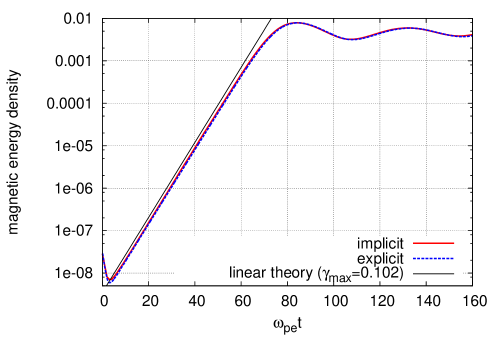
Figure 2: Time history of the magnetic field energy evolving from an electron Weibel instability. Excellent agreement is found between explicit (with $32\times 32$ uniform cells, $\Delta t=0.05$), implicit, and the theoretical linear growth rate. In the linear stage, the magnetic field energy grows as $W_{A}=W_{A0}\mathrm{exp}(2\gamma\omega_{pe}t)$.

The time history of conserved quantities (e.g., charge, energy, momentum, canonical momenta, and $\nabla\cdot\mathbf{A}$) of the simulated system is depicted in Fig. 3,

Figure 3: Conserved quantities in the simulation of the electron Weibel instability. Charge conservation is measured as the (root-mean-square) rms of the continuity equation, numerically evaluated at grid cells $\sqrt{\sum_{i=1}^{N_{g}}(\rho_{i}^{n+1}-\rho_{i}^{n}+\Delta t(\bar{j}_{i+\nicefrac{{1}}{{2}}}-\bar{j}_{i-\nicefrac{{1}}{{2}}})/\Delta x)^{2}}$, where $N_{g}$ is the number of grid-points. Energy conservation is measured as the accumulated change in the total energy (c.f. Eq. 52) with respect to the initial one. Momentum conservation in the $x$ direction is measured as $\sum_{p}m_{p}v_{p,x}/\sum_{p}m_{p}v_{th,x}$, with $p$ the particle index respectively. The maximum error in the conservation of canonical momenta for all particles is measured as $\max_{p}\left(\mid m_{p}v_{p}^{n+1}+q_{p}A_{p}^{n+1}-m_{p}v_{p}^{n}-q_{p}A_{p}^{n}\mid\right)$ in the $z$ direction. Finally, the rms of $\nabla\cdot\mathbf{A}$ is found as $\sqrt{\sum_{ij}^{N_{g}}\left[(A_{xi+\nicefrac{{1}}{{2}},j}-A_{xi-\nicefrac{{1}}{{2}},j})/\Delta x+(A_{yi,j+\nicefrac{{1}}{{2}}}-A_{yi,j-\nicefrac{{1}}{{2}}})/\Delta y)\right]^{2}}$.

for both implicit and explicit computations. We see that charge conservation is preserved at round-off level for both explicit and implicit algorithms. For the implicit computation, energy conservation is controlled by the JFNK nonlinear tolerance (a relative tolerance of $10^{-6}$ in used in this study), and the canonical momenta conservation is controlled by the Picard tolerance level for orbit integration (an absolute tolerance of $10^{-12}$ is used). With respect to exact energy and canonical momentum conservation, we see that the implicit computation out-performs the explicit one by many orders of magnitude. As in earlier studies [20], the particle momentum in the $x$-direction is not conserved exactly, but the error is relatively small. The momentum conservation is slightly better in the explicit computations, likely due to the use of a much smaller time step. Finally, as expected, $\nabla\cdot\mathbf{A}$ is well conserved in both algorithms. Explicit results are close to round-off level; implicit results are dependent on the nonlinear tolerance, owing to exact charge conservation and our involution-free Vlasov-Darwin formulation.

5.1.1 Temporal convergence study

We have performed a temporal convergence study of the CN-based implicit PIC scheme. Numerical experiments use a fixed $\Delta x$ and a series of timesteps ($\Delta t$). We record the solutions at final times, $t=8$. Relative numerical errors are obtained by comparing the result of these solutions with a reference solution (obtained by using a small timestep $\Delta t=4\times 10^{-4}$). Results are shown in Fig. 4.

Figure 4: Numerical convergence rate of the CN scheme. Second-order scalings are verified for both $\phi$ and $\mathbf{A}$. The $y$-axis is defined as the relative error $[Q(\Delta t)-Q_{ref}]/Q_{ref}$, where $Q$ is the $L_{2}$-norm of the solution.

We confirm the second-order temporal scaling of the error for both $\mathbf{A}$ and $\phi$, as expected from the time-centered CN scheme employed in the algorithm in both the field and particle governing equations.

5.1.2 Preconditioner performance

We use the Weibel test example, with various mass ratios and grid sizes, to evaluate the performance of the fluid preconditioner proposed in Sec. 4. We test the solver performance with and without preconditioning. The number of linear and nonlinear iterations per time step are monitored and averaged over 10 timesteps. A key figure of merit is the number of function evaluations ($N_{FE}$), found from the sum of linear and nonlinear iterations ($N_{FE}$ equals the number of calls to the particle integration routine).

Table 1: Solver performance with and without the fluid preconditioner for the electron Weibel case with $L_{x}\times L_{y}=22\times 22$ ($d_{e}^{2}$), $N_{x}\times N_{y}=128\times 128$, and $N_{pc}=200$. For all the test cases, $\Delta t=0.1\omega_{pi}^{-1}$. The Newton and GMRES iteration numbers reported are per time step, averaged over 10 timesteps.

$m_{i}/m_{e}$	no preconditioner		with preconditioner
	Newton	GMRES	Newton	GMRES
25	5.8	192.5	3	0
100	5.7	188.8	3	0
1836	7.7	237.8	4	2.8

Table 1 shows the solver performance with respect to the mass ratio. The number of nonlinear (Newton) iterations is a function of the nonlinear tolerance (which is $10^{-6}$ in this study), and is about 4 to 7 upon convergence. For the unpreconditioned case, the number of linear (GMRES) iterations increases with the ion-electron mass ratio. This is expected, because the problem becomes stiffer (the electron plasma frequency becomes larger) when $\Delta t$ is pegged to the ion plasma frequency. With preconditioning, the solver convergence rate is essentially independent of the mass ratio, confirming the asymptotic analysis in Sec. 4.3. We note that, because we use the preconditioner to provide the initial guess for the GMRES solver, sometimes no GMRES iterations are needed for convergence. The improvement in the solver convergence rate (measured by $N_{FE}$) achieved by the fluid preconditioner is between 30 and 60.

Table 2: Solver performance with and without the fluid preconditioner for the electron Weibel case with the various mesh sizes (keeping $m_{i}/m_{e}=1836$ and other parameters the same as used for Table 1).

$N_{x}\times N_{y}$	no preconditioner		with preconditioner
	Newton	GMRES	Newton	GMRES
$16\times 16$	3.7	20	3	0.9
$32\times 32$	4	38.5	3	0.9
$64\times 64$	4.3	79.9	3	0.2

Table 2 shows the solver performance with respect to the grid resolution for $m_{i}/m_{e}=1836$. While the unpreconditioned case is very sensitive to grid refinement, the preconditioned solver is not sensitive at all (owing to the use of MG solvers in the preconditioner). The improvement in the solver convergence rate achieved by the fluid preconditioner is again large, of more than two orders of magnitude.

As will be demonstrated in the next section, the preconditioner performance is also robust against variations in the domain size: the number of Newton iterations is about 3 to 4 and the number of GMRES iterations is about 1 to 3 when we vary the domain size $L$ by three orders of magnitude. This also confirms the asymptotic analysis in Sec. 4.3.

5.1.3 CPU speedup of implicit vs. explicit PIC

The efficiency advantage of the implicit PIC approach vs. the explicit one is summarized in Eq. 60 of Ref. [22], repeated here for convenience:

$$\frac{CPU_{ex}}{CPU_{imp}}\sim\frac{0.02}{(k\lambda_{D})^{d}}\frac{c}{v_{A}}\min\left[\frac{1}{k\lambda_{D}},\frac{c}{v_{A}}\sqrt{\frac{m_{e}}{m_{i}}},\sqrt{\frac{m_{i}}{m_{e}}}\right]\frac{1}{N_{FE}{\color[rgb]{1,0,0}{\color[rgb]{0,0,0}N}_{{\color[rgb]{0,0,0}Picard}}}}.$$ (108)

In Eq. 108, $k=2\pi/L$, $d_{e}$ is the electron skin depth, $N_{FE}$ is the number of function evaluations (which indicates the number of repeated particle orbit computations), and $N_{Picard}$ is the number of Picard iteration for orbit integration. We see that the speedup increases with larger domain sizes (where $k\lambda_{D}\ll 1$, $d_{e}\gg\lambda_{D}$), and with $m_{i}$ much larger than $m_{e}$. Here, we vary the domain size $L$. It is expected that the cost of the implicit simulation will not change much with the domain size, provided that the number of cells and particles per cell are kept fixed, and the nonlinear iteration count is well controlled by the preconditioner. On the other hand, the explicit code is forced to maintain the same grid spacing and time step as the domain increases, to avoid numerical instability.

Results are depicted in Fig. 5,

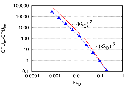
Figure 5: CPU speedup of implicit vs. explicit PIC for the electron Weibel instability case as a function of $k\lambda_{D}\sim\lambda_{D}/L$. Speedups of several orders of magnitude are possible for large domains ($\lambda_{D}/L\ll 1$).

and show that the speedup ($CPU_{ex}/CPU_{im}$) is closely proportional to $(k\lambda_{D})^{-3}$ for small domain sizes, in agreement with Eq. 108 (for $d=2$, and $\frac{1}{k\lambda_{D}}<\sqrt{\frac{m_{i}}{m_{e}}}$). As $L$ increases (or $k\lambda_{D}$ decreases), the scaling index becomes $\sim 2$, as expected from the same equation. The scaling index changes at $\frac{1}{k\lambda_{D}}\sim\sqrt{\frac{m_{i}}{m_{e}}}\simeq 0.025$, also expected (note that $c/v_{A}\gg 1$ in this example, since it is weakly magnetized). Overall, these results are in a good agreement with our simple estimate. Significant CPU speedups are possible for system sizes much larger than the Debye length ($>10^{4}$ for $k\lambda_{D}<10^{-3}$).

5.2 The kinetic Alfvén wave ion-ion streaming instability

For our second test, we consider the excitation of kinetic Alfvén waves (KAW) by ion-ion streaming in 2D-3V [54]. This is a moderately magnetized case, with an imposed external magnetic field. The instability is caused by interactions between the wave and the streaming ions. The simulation parameters are similar to those used in Ref. [54]. The mass ratio is $m_{i}/m_{e}=25$, which is nominal (we will vary this parameter later). We use ions as the reference species. The simulated domain is $10(d_{i})\times 10(d_{i})$ (the unit length being the ion skin depth), with $64\times 64$ uniformly distributed cells (with each cell size in each direction about 10 times larger than the Debye length) and periodic boundary conditions, and the average number of particles per cell of one species is 500. The external magnetic field is set to be $B_{0}=0.0667$ along the $x$-axis. The plasma consists of Maxwellian electrons with $v_{eT}=0.0745$ ($\beta_{e}=0.1)$, and two singly charged ion components, i.e., an ambient ion component $a$ and an ion beam component $b$, with number densities $n_{a}=0.6n_{e}$ and $n_{b}=0.4n_{e}$ (where $n_{e}$ is the electron density). The two ion components have $v_{aT}=1.925\times 10^{-2}$ and $v_{bT}=7.45\times 10^{-3}$, and a relative streaming speed with respect to each other of $v_{ad}=1.5v_{A}$, and $v_{bd}=v_{A}$, with $v_{A}=\sqrt{m_{e}/m_{i}}/3$ the Alfvén speed along the external magnetic field direction. The timestep is again set to $\Delta t=0.1\omega_{pi}^{-1}$ (about 10 times larger than the explicit CFL for the mass ratio considered). The simulation is started without perturbing a specific wavelength. Consequently, waves with all wavelengths and with all angles to $B_{0}$ supported by the simulation domain are excited. Figure 6 shows the simulation result of the magnetic energy density, which is again in excellent agreement with linear theory (the growth rate for this configuration is found to be $\gamma=0.225$, using the same linear Vlasov code as in Ref. [55]).

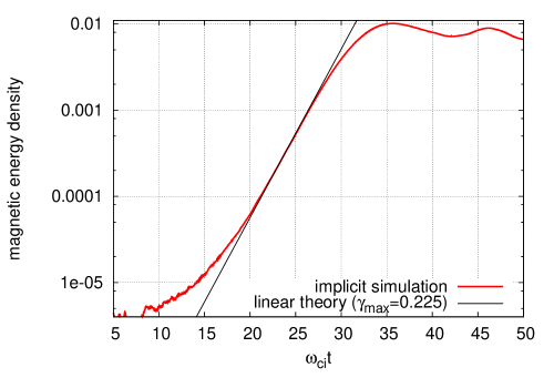
Figure 6: Time history of the magnetic field energy for the KAW simulation, demonstrating excellent agreement with linear theory.

5.2.1 Preconditioner performance

Table 3: Solver performance for the KAW case with and without preconditioning for $L_{x}\times L_{y}=22$($d_{i}$)$\times 22$($d_{i}$), $N_{x}\times N_{y}=32\times 32$, and $N_{pc}=200$. For all the test cases, $\Delta t=0.1\omega_{pi}^{-1}$. Convergence data is averaged over 10 time steps.

$m_{i}/m_{e}$	no preconditioner		with preconditioner
	Newton	GMRES	Newton	GMRES
25	4	171.9	3.2	1
150	4.5	764	4	2.9
600	7.4	4054.8	4	11.9

Table 3 shows the solver performance with respect to the mass ratio for the KAW test. From these results, it is clear that the solver performance is much more sensitive to the mass ratio in this example, since both unpreconditioned and preconditioned solvers degrade with the mass ratio (although the preconditioned one degrades less). The origin of the performance degradation is the moderately magnetized nature of this test case: as the mass ratio increases, the condition $\omega_{pe}>\omega_{ce}$ (see Sec.4) is violated, thus leading to the performance degradation. To confirm this behavior, we conduct a slightly different test, where we fix $\omega_{pe}/\omega_{ce}=3$ by reducing $B_{0}$ as we increase the mass ratio.

Table 4: Solver performance for the KAW case with and without preconditioning, with fixed $\omega_{pe}/\omega_{ce}=3$. Other parameters are the same as in Table 3. (NC denotes “no convergence”.)

$m_{i}/m_{e}$	no preconditioner		with preconditioner
	Newton	GMRES	Newton	GMRES
150	4.5	738	4	3
600	5.8	1887	4	3.9
1836	NC	NC	4	5.9
7344	NC	NC	4	12.9

The results are shown in Table 4. As the mass ratio increases from 150 to 1836, $\omega_{ce}\Delta t$ increases from 0.4 to 1.4, and the performance of the preconditioner remains reasonably bounded. The performance degrades with the mass ratio as it increases further by a factor of 4, with the number of GMRES iterations approximately proportional to $\omega_{ce}\Delta t$ $(\simeq 3$). The reason is that, in this regime, electron Bernstein modes are excited at multiples of $\omega_{ce}$, which are not captured by the moment preconditioner proposed in this study. The performance recovers with a reduced time step, when Bernstein modes are resolved (for instance, the number of GMRES iterations is about 4 and 6 for $\omega_{ce}\Delta t=1$ and $1.5$, respectively).

6 Discussion and conclusions

In this study, we have developed a two-dimensional, conservative, fully implicit PIC algorithm for the (non-radiative) Vlasov-Darwin equation set. The approach builds on (and generalizes) a previous successful 1D implementation [22]. Nonlinear convergence between particles and fields is enforced to a tight nonlinear tolerance via a multigrid preconditioned Jacobian-free Newton-Krylov solver. Particles are enslaved in the nonlinear function, so they do not appear explicitly as dependent variables in the nonlinear residual. As a result, the nonlinear solver only iterates on fields, resulting in a much reduced memory footprint. Only one copy of the particle population is needed by the algorithm. The algorithmic advantage of the fully implicit scheme is its absolute stability, which relaxes the numerical instability constraints of conventional explicit schemes. This is especially beneficial for large-scale simulations, with system sizes much larger than the electron Debye length.

The formulation conserves exactly local charge, total energy, and the canonical momentum component in the ignorable direction. It also automatically preserves exactly the two involutions in the discrete, namely, Gauss’s law and the Coulomb gauge (the latter being critical for energy conservation). This is accomplished by the minimum set of $(\mathbf{A}-\phi)$ equations proposed in this study. A (2nd-order) space-time-centered finite-difference scheme, together with compatible interpolations with multi-D shape functions, are key to achieve simultaneous conservation of local charge, global energy, and canonical momentum.

The nonlinear, multidimensional, implicit kinetic algorithm is accelerated with a moment-based preconditioner. The preconditioner assumes a moderately magnetized regime where $\omega_{p,e}>\omega_{c,e}$, and is formulated such that it features the correct asymptotic limits for arbitrarily small electron mass (ambipolar limit) and arbitrarily large domains (MHD limit). The resulting linear systems are effectively inverted using multigrid methods, which lend the approach a grid-independent convergence rate. Solver performance is also largely independent of the electron mass, except when the plasma becomes strongly magnetized. In strongly magnetized regimes, performance is recovered when $\omega_{ce}\Delta t\simeq 1$.

The algorithm has been verified against an explicit Vlasov-Maxwell solver, and against linear theory growth rate predictions, without resolving the Debye length or plasma wave frequency. A back of the envelope estimate for the explicit-to-implicit CPU speedup predicts that significant speedups are possible when $\lambda_{D}/L\ll 1$. Specifically, for sufficiently small values of $\lambda_{D}/L$, the CPU speedup scales as $(L/\lambda_{D})^{d}$, which can be a very large number. Numerical experiments in this study have demonstrated speedups of more than four orders of magnitude.

Future work will focus on extending the preconditioner to strongly magnetized regimes, and to generalize the solver to curvilinear geometry (as was done in the electrostatic case in Ref. [56]).

Appendix A Explicit Vlasov-Maxwell solver

We briefly describe the explicit scheme implemented in this study. The scheme is almost the same as that proposed in Appendix B of Ref. [57], except for aspects of charge conservation. We begin with Maxwell’s equations in the ($\mathbf{A}-\phi$) formulation:

$$\frac{1}{\mu_{0}}\nabla^{2}\mathbf{A}+\mathbf{j}-\epsilon_{0}\partial_{t}\nabla\phi-\epsilon_{0}\frac{\partial^{2}\mathbf{A}}{\partial t^{2}} = 0,$$ (109)

$$\epsilon_{0}\nabla^{2}\phi+\rho = 0,$$ (110)

together with the leapfrog particle pusher to advance ($x_{p},v_{p}$) for all particles. Equations 109, 110 are discretized with central differences in time and space to obtain:

$$\frac{1}{\mu_{0}}(\delta_{x}^{2}+\delta_{y}^{2})\left(\begin{array}[]{c}[A_{x}]_{i+\nicefrac{{1}}{{2}},j}\\ {}[A_{y}]_{i,j+\nicefrac{{1}}{{2}}}\\ {}[A_{z}]_{i,j}\end{array}\right)^{n}+\left(\begin{array}[]{c}[\bar{j_{x}}]_{i+\nicefrac{{1}}{{2}},j}\\ {}[\bar{j_{y}}]_{i,j+\nicefrac{{1}}{{2}}}\\ {}[\bar{j_{z}}]_{i,j}\end{array}\right)^{n} = \epsilon_{0}\delta_{t}\left(\begin{array}[]{c}\delta_{x}[\phi]_{i+\nicefrac{{1}}{{2}},j}\\ \delta_{y}[\phi]_{i,j+\nicefrac{{1}}{{2}}}\\ 0\end{array}\right)^{n}+\epsilon_{0}\delta_{t}^{2}\left(\begin{array}[]{c}[A_{x}]_{i+\nicefrac{{1}}{{2}},j}\\ {}[A_{y}]_{i,j+\nicefrac{{1}}{{2}}}\\ {}[A_{z}]_{i,j}\end{array}\right)^{n},$$ (123)

$$\epsilon_{0}(\delta_{x}^{2}+\delta_{y}^{2})[\phi]_{i,j}^{n+\nicefrac{{1}}{{2}}} = [\rho]_{i,j}^{n+\nicefrac{{1}}{{2}}},$$ (124)

where $\delta_{t}^{2}[A]^{n}\equiv(A^{n+1}-2A^{n}+A^{n-1})/\Delta t^{2}$, and $\delta_{t}[\phi]^{n}=(\phi^{n+\nicefrac{{1}}{{2}}}-\phi^{n-\nicefrac{{1}}{{2}}})/\Delta t$. All the other finite-difference notations are the same as those introduced in Sec. 3. The time-integration of the whole system is performed in a leapfrog fashion, with $\mathbf{A}$ and $v_{p}$ defined at integer time levels, and $\phi$ and $x_{p}$ at half-time levels.

The basic procedure for advancing the code for one time step is the following. At the beginning of each time step, we have the particles at ($x_{p}^{n-\nicefrac{{1}}{{2}}},v_{p}^{n-1}$), the vector potential for the two previous steps ($\mathbf{A}^{n-1},\mathbf{A}^{n}$), the static potential at $\phi^{n-\nicefrac{{1}}{{2}}}$, and the fields ($\mathbf{B}^{n-\nicefrac{{1}}{{2}}},\mathbf{E}^{n-\nicefrac{{1}}{{2}}}$). Then, we perform the following steps:

1. Advance particles to ($x_{p}^{n+\nicefrac{{1}}{{2}}},v_{p}^{n}$), and accumulate the densities $\rho^{n+\nicefrac{{1}}{{2}}}$ and $j^{n}$ on the grid.

2. Solve Eq. 124 for $\phi^{n+\nicefrac{{1}}{{2}}}$.

3. Solve Eq. 123 for $\mathbf{A}^{n+1}$.

To get the simulation started, we assume $\left.\frac{\partial\mathbf{A}}{\partial t}\right|_{t=0}=0$, and find ($\mathbf{A},\phi$) at $t=0$ using the Darwin approximation (by solving Eq. 18 and 124; note that the initial $\delta_{t}\phi$ is found from the solution of these equations). We use the velocity at $t=0$ to reverse the particle position to $t=-\frac{1}{2}$, and then the above procedure can be used to advance the whole system.

For exact charge conservation, we combine the charge-current interpolation scheme (Eqs. 21-23, 47) employed in this study with the cell-crossing scheme introduced by Ref. [49]. It is sufficient to focus the discussion on one particle substep from $t^{n-\nicefrac{{1}}{{2}}}$ to $t^{n+\nicefrac{{1}}{{2}}}$ (the total charge is found by linear superposition of all particles). Note exact charge conservation is automatic if the particle substep is within a cell. When a particle crosses one or several cells in a single time step, we split the trajectory into several segments $\nu=1$, $N^{\nu}$, separated by cell faces. For each segment, we compute position updates ($\Delta x_{p}^{\nu+\nicefrac{{1}}{{2}}}$,$\Delta y_{p}^{\nu+\nicefrac{{1}}{{2}}}$)=($x_{p}^{\nu+1}-x_{p}^{\nu}$,$y_{p}^{\nu+1}-y_{p}^{\nu}$) and partial contributions to the current density as:

$$(j_{p,x})_{i+\nicefrac{{1}}{{2}},j}^{\nu+\nicefrac{{1}}{{2}}} = \frac{1}{\Delta t}\frac{q_{p}}{\Delta x\Delta y}\Delta x_{p}^{\nu+\nicefrac{{1}}{{2}}}S_{2}^{\nu+\nicefrac{{1}}{{2}}}(y_{p}-y_{j})S_{1}(x_{p}^{\nu+\nicefrac{{1}}{{2}}}-x_{i+\nicefrac{{1}}{{2}}}),$$ (125)

$$(j_{p,y})_{i,j+\nicefrac{{1}}{{2}}}^{\nu+\nicefrac{{1}}{{2}}} = \frac{1}{\Delta t}\frac{q_{p}}{\Delta x\Delta y}\Delta y_{p}^{\nu+\nicefrac{{1}}{{2}}}S_{2}^{\nu+\nicefrac{{1}}{{2}}}(x_{p}-x_{i})S_{1}(y_{p}^{\nu+\nicefrac{{1}}{{2}}}-y_{j+\nicefrac{{1}}{{2}}}),$$ (126)

where $x_{p}^{\nu+\nicefrac{{1}}{{2}}}=(x_{p}^{\nu+1}+x_{p}^{\nu})/2$ and $y_{p}^{\nu+\nicefrac{{1}}{{2}}}=(y_{p}^{\nu+1}+y_{p}^{\nu})/2$. Note that the interpolations are identical to those of the implicit scheme (Eqs. 22, 21). The total current density is obtained by summing up all partial contributions for all particles (very similarly to the orbit-averaging procedure in the implicit case):

$$\bar{j}_{x(y)}=\sum_{p}\sum_{\nu=0}^{N_{\nu}-1}j_{p,x(y)}^{\nu+\nicefrac{{1}}{{2}}}.$$

For the $z$-direction, since there is no cell-crossing, we simply have

$$\bar{j}_{z}=\sum_{p}\frac{q_{p}}{\Delta x\Delta y}v_{pz}^{n}S_{2}^{n+\nicefrac{{1}}{{2}}}(x_{p}-x_{i})S_{2}^{n+\nicefrac{{1}}{{2}}}(y_{p}-y_{j+\nicefrac{{1}}{{2}}}).$$

Almost exactly the same procedure outlined in Sec. 3.1 can be used to prove that the following charge conservation equation is satisfied:

$$\frac{(\rho)_{i,j}^{n+\nicefrac{{1}}{{2}}}-(\rho)_{i,j}^{n-\nicefrac{{1}}{{2}}}}{\Delta t}+\frac{(\bar{j}_{x})_{i+\nicefrac{{1}}{{2}},j}-(\bar{j}_{x})_{i-\nicefrac{{1}}{{2}},j}}{\Delta x}+\frac{(\bar{j}_{y})_{i,j+\nicefrac{{1}}{{2}}}-(\bar{j}_{y})_{i,j-\nicefrac{{1}}{{2}}}}{\Delta y}=0.$$ (127)

With Eqs. 127 and 123-124 being satisfied, it is straightforward to prove (by taking the numerical divergence of Eq. 123) that $\nabla\cdot\mathbf{A}=0$ is also satisfied numerically at all times if it is satisfied initially.

References

• [1] C. K. Birdsall and A. B. Langdon, Plasma Physics via Computer Simulation. New York: McGraw-Hill, 2005.
• [2] R. W. Hockney and J. W. Eastwood, Computer Simulation Using Particles. Bristol, UK: Taylor & Francis, Inc, 1988.
• [3] L. Landau and E. Lifshitz, “The classical theory of fields,” 1951.
• [4] B. B. Godfrey, “Numerical Cherenkov instabilities in electromagnetic particle codes,” Journal of Computational Physics, vol. 15, no. 4, pp. 504–521, 1974.
• [5] A. B. Langdon, “Some electromagnetic plasma simulation methods and their noise properties,” Physics of Fluids, vol. 15, p. 1149, 1972.
• [6] S. Markidis and G. Lapenta, “The energy conserving particle-in-cell method,” Journal of Computational Physics, vol. 230, no. 18, pp. 7037–7052, 2011.
• [7] C. W. Nielson and H. R. Lewis, “Particle-code models in the nonradiative limit,” Methods in Computational Physics, vol. 16, pp. 367–388, 1976.
• [8] J. Busnardo-Neto, P. Pritchett, A. Lin, and J. Dawson, “A self-consistent magnetostatic particle code for numerical simulation of plasmas,” Journal of Computational Physics, vol. 23, no. 3, pp. 300–312, 1977.
• [9] J. Byers, B. Cohen, W. Condit, and J. Hanson, “Hybrid simulations of quasineutral phenomena in magnetized plasma,” Journal of Computational Physics, vol. 27, no. 3, pp. 363–396, 1978.
• [10] D. Hewett, “Low-frequency electromagnetic (Darwin) applications in plasma simulation,” Computer physics communications, vol. 84, no. 1, pp. 243–277, 1994.
• [11] M. Gibbons and D. Hewett, “The Darwin Direct Implicit Particle-in-Cell (DADIPIC) method for simulation of low frequency plasma phenomena,” Journal of Computational Physics, vol. 120, pp. 231–247, 1995.
• [12] E. Sonnendrücker, J. J. Ambrosiano, and S. T. Brandon, “A finite element formulation of the Darwin PIC model for use on unstructured grids,” Journal of Computational Physics, vol. 121, no. 2, pp. 281–297, 1995.
• [13] W. Lee, H. Qin, and R. C. Davidson, “Nonlinear perturbative electromagnetic (Darwin) particle simulation of high intensity beams,” Nuclear Instruments and Methods in Physics Research Section A: Accelerators, Spectrometers, Detectors and Associated Equipment, vol. 464, no. 1, pp. 465–469, 2001.
• [14] T. Taguchi, T. Antonsen Jr, and K. Mima, “Study of hot electron beam transport in high density plasma using 3D hybrid-Darwin code,” Computer physics communications, vol. 164, no. 1, pp. 269–278, 2004.
• [15] L. V. Borodachev, I. Mingalev, and O. Mingalev, “The numerical approximation of discrete Vlasov-Darwin model based on the optimal reformulation of field equations,” Matematicheskoe Modelirovanie, vol. 18, no. 11, pp. 117–125, 2006.
• [16] D. Eremin, T. Hemke, R. P. Brinkmann, and T. Mussenbrock, “Simulations of electromagnetic effects in high-frequency capacitively coupled discharges using the Darwin approximation,” Journal of Physics D: Applied Physics, vol. 46, no. 8, p. 084017, 2013.
• [17] H. Schmitz and R. Grauer, “Darwin–vlasov simulations of magnetised plasmas,” Journal of Computational Physics, vol. 214, no. 2, pp. 738–756, 2006.
• [18] H. Weitzner and W. S. Lawson, “Boundary conditions for the Darwin model,” Physics of Fluids B: Plasma Physics, vol. 1, p. 1953, 1989.
• [19] P. Degond and P.-A. Raviart, “An analysis of the Darwin model of approximation to Maxwell’s equations,” Forum Math, vol. 4, no. 4, pp. 13–44, 1992.
• [20] G. Chen, L. Chacón, and D. C. Barnes, “An energy- and charge-conserving, implicit, electrostatic particle-in-cell algorithm,” Journal of Computational Physics, vol. 230, pp. 7018–7036, 2011.
• [21] W. T. Taitano, D. A. Knoll, L. Chacón, and G. Chen, “Development of a consistent and stable fully implicit moment method for vlasov–ampère particle in cell (pic) system,” SIAM Journal on Scientific Computing, vol. 35, no. 5, pp. S126–S149, 2013.
• [22] G. Chen and L. Chacon, “An energy-and charge-conserving, nonlinearly implicit, electromagnetic 1D-3V Vlasov–Darwin particle-in-cell algorithm,” Computer Physics Communications, vol. 185, no. 10, pp. 2391–2402, 2014.
• [23] D. A. Knoll and D. E. Keyes, “Jacobian-free Newton–Krylov methods: a survey of approaches and applications,” Journal of Computational Physics, vol. 193, no. 2, pp. 357–397, 2004.
• [24] G. Chen, L. Chacon, C. A. Leibs, D. A. Knoll, and W. Taitano, “Fluid preconditioning for Newton-Krylov-based, fully implicit, electrostatic particle-in-cell simulations,” Journal of computational physics, vol. 258, p. 555, 2014.
• [25] G. Chen, L. Chacón, and D. C. Barnes, “An efficient mixed-precision, hybrid cpu-gpu implementation of a nonlinearly implicit one-dimensional particle-in-cell algorithm,” Journal of Computational Physics, vol. 231, no. 16, pp. 5374–5388, 2012.
• [26] R. J. Mason, “Implicit moment particle simulation of plasmas,” J. Comput. Phys., vol. 41, no. 2, pp. 233 – 244, 1981.
• [27] J. Denavit, “Time-filtering particle simulations with $\omega_{pe}\Delta t\gg 1$,” J. Comput. Phys., vol. 42, no. 2, pp. 337 – 366, 1981.
• [28] J. U. Brackbill and D. W. Forslund, “An implicit method for electromagnetic plasma simulation in two dimensions,” Journal of Computational Physics, vol. 46, p. 271, 1982.
• [29] J. Brackbill and D. Forslund, “Simulation of low-frequency electromagnetic phenomena in plasmas,” in Multiple time scales (J. U. Brackbill and B. I. Cohen, eds.), Academic Press, 1985.
• [30] H. Vu and J. Brackbill, “CELEST1D: an implicit, fully kinetic model for low-frequency, electromagnetic plasma simulation,” Comput. Phys. Commun., vol. 69, p. 253, 1992.
• [31] G. Lapenta and J. Brackbill, “CELESTE 3D: Implicit adaptive grid plasma simulation,” in International School/Symposium for Space Simulation, (Kyoto, Japan), March 13-19 1997.
• [32] A. Friedman, A. B. Langdon, and B. I. Cohen, “A direct method for implicit particle-in-cell simulation,” Comments on plasma physics and controlled fusion, vol. 6, no. 6, pp. 225 – 36, 1981.
• [33] A. B. Langdon, B. I. Cohen, and A. Friedman, “Direct implicit large time-step particle simulation of plasmas,” J. Comput. Phys., vol. 51, no. 1, pp. 107 – 38, 1983.
• [34] A. B. Langdon and D. C. Barnes, “Direct implicit plasma simulation,” in Multiple time scales (J. U. Brackbill and B. I. Cohen, eds.), pp. 335–375, Academic Press, New York, 1985.
• [35] D. W. Hewett and A. B. Langdon, “Electromagnetic direct implicit plasma simulation,” J. Comput. Phys., vol. 72, no. 1, pp. 121 – 55, 1987.
• [36] T. Kamimura, E. Montalvo, D. C. Barnes, J. N. Leboeuf, and T. Tajima, “Implicit particle simulation of electromagnetic plasma phenomena,” Journal of Computational Physics, vol. 100, no. 1, pp. 77–90, 1992.
• [37] D. W. Hewett, “Elimination of electromagnetic radiation in plasma simulation: The Darwin or magnetoinductive approximation,” Space Science Reviews, vol. 42, pp. 29–40, 1985.
• [38] P.-A. Raviart and E. Sonnendrücker, “A hierarchy of approximate models for the Maxwell equations,” Numerische Mathematik, vol. 73, no. 3, pp. 329–372, 1996.
• [39] T. B. Krause, A. Apte, and P. Morrison, “A unified approach to the Darwin approximation,” Physics of Plasmas, vol. 14, p. 102112, 2007.
• [40] C. M. Dafermos, “Hyperbolic conservation laws in continuum physics, volume 325 of grundlehren der mathematischen wissenschaften [fundamental principles of mathematical sciences],” 2000.
• [41] T. Barth, “On the role of involutions in the discontinuous galerkin discretization of maxwell and magnetohydrodynamic systems,” in Compatible spatial discretizations, pp. 69–88, Springer, 2006.
• [42] B.-N. Jiang, J. Wu, and L. A. Povinelli, “The origin of spurious solutions in computational electromagnetics,” Journal of computational physics, vol. 125, no. 1, pp. 104–123, 1996.
• [43] A. Hasegawa and H. Okuda, “One-dimensional plasma model in the presence of a magnetic field,” Physics of Fluids, vol. 11, p. 1995, 1968.
• [44] J. Boris, “Relativistic plasma simulation-optimization of a hybrid code,” in Proc. Fourth Conf. Num. Sim. Plasmas, Naval Res. Lab, Wash. DC, pp. 3–67, 1970.
• [45] C.-D. Munz, P. Omnes, R. Schneider, E. Sonnendrücker, and U. Voss, “Divergence correction techniques for maxwell solvers based on a hyperbolic model,” Journal of Computational Physics, vol. 161, no. 2, pp. 484–511, 2000.
• [46] G. Chen, L. Chacón, and D. C. Barnes, “An energy-conserving nonlinearly converged implicit particle-in-cell (PIC) algorithm,” in Bull. Am. Phys. Soc., vol. 55 (15), November 2010. Abstract TP9.34.
• [47] H. Vu and J. Brackbill, “Accurate numerical solution of charged particle motion in a magnetic field,” Journal of Computational Physics, vol. 116, no. 2, pp. 384–387, 1995.
• [48] G. Chen and L. Chacón, “An analytical particle mover for the charge-and energy-conserving, nonlinearly implicit, electrostatic particle-in-cell algorithm,” Journal of Computational Physics, vol. 247, pp. 79–87, 2013.
• [49] J. Villasenor and O. Buneman, “Rigorous charge conservation for local electromagnetic field solvers,” Comput. Phys. Commun., vol. 69, pp. 306–316, 1992.
• [50] A. N. Kaufman and P. S. Rostler, “The Darwin model as a tool for electromagnetic plasma simulation,” Physics of Fluids, vol. 14, p. 446, 1971.
• [51] H. Goldstein, “Classical mechanics,” 1980.
• [52] T. M. C. Leibs, “Nested iteration and first-order system least squares for two-fluid electromagnetic darwin model,” SIAM Journal on Scientific Computing, 2015, submitted.
• [53] N. A. Krall and A. W. Trivelpiece, Principles of plasma physics. International Student Edition-International Series in Pure and Applied Physics, Tokyo: McGraw-Hill Kogakusha, 1973.
• [54] L. Yin, D. Winske, W. Daughton, and K. Bowers, “Kinetic Alfvén waves and electron physics. I. Generation from ion-ion streaming,” Physics of plasmas, vol. 14, no. 6, pp. 062104–062104, 2007.
• [55] W. Daughton and S. P. Gary, “Electromagnetic proton/proton instabilities in the solar wind,” Journal of Geophysical Research: Space Physics (1978–2012), vol. 103, no. A9, pp. 20613–20620, 1998.
• [56] L. Chacón, G. Chen, and D. Barnes, “A charge-and energy-conserving implicit, electrostatic particle-in-cell algorithm on mapped computational meshes,” Journal of Computational Physics, vol. 233, pp. 1–9, 2013.
• [57] R. L. Morse and C. W. Nielson, “Numerical simulation of the Weibel instability in one and two dimensions,” Phys. Fluids, vol. 14, p. 830, 1971.