Geometric Adaptive Control for Aerial Transportation of a Rigid Body

Taeyoung Lee Taeyoung Lee, Mechanical and Aerospace Engineering, George Washington University, Washington, DC 20052 tylee@gwu.eduThis research has been supported in part by NSF under the grants CMMI-1243000 (transferred from 1029551), CMMI-1335008, and CNS-1337722.
Abstract

This paper is focused on tracking control for a rigid body payload, that is connected to an arbitrary number of quadrotor unmanned aerial vehicles via rigid links. A geometric adaptive controller is constructed such that the payload asymptotically follows a given desired trajectory for its position and attitude in the presence of uncertainties. The coupled dynamics between the rigid body payload, links, and quadrotors are explicitly incorporated into control system design and stability analysis. These are developed directly on the nonlinear configuration manifold in a coordinate-free fashion to avoid singularities and complexities that are associated with local parameterizations.

I Introduction

By utilizing the high thrust-to-weight ratio, quadrotor unmanned aerial vehicles have been envisaged for aerial load transportation [1, 2, 3]. Most of the existing results for the control of quadrotors to transport a cable-suspended payload are based on the assumption that the dynamics of the payload is decoupled from the dynamics of quadrotors. For example, the effects of the payload are considered as arbitrary external force and torque exerted to quadrotors [2]. As such, these results may not be suitable for agile load transportation where the motion of cable and payload should be actively suppressed.

Recently, the full dynamic model for an arbitrary number of quadrotors transporting a payload are developed, and based on that, geometric tracking controllers are constructed in an intrinsic fashion. In particular, autonomous transportation of a point mass connected to quadrotors via rigid links is developed in [4]. It has been generalized into a more realistic dynamic model that considers the deformation of cables in [5], and also the attitude dynamics of a payload, that is considered as a rigid body instead of a point mass, is incorporated in [6]. However, these results are based on the assumption that the exact properties of the quadrotors and the payload are available, and that there are no external disturbances, thereby making it challenging to implement those results in actual hardware systems.

The objective of this paper is to construct a control system for an arbitrary number of quadrotors connected to a rigid body payload via rigid links with explicit consideration on uncertainties. A coordinate-free form of the equations of motion that have been developed in [6] is extended to include the effects of unknown, but fixed forces and moments acting on each of the quadrotors, the cables, and the payload. A geometric nonlinear adaptive control system is designed such that both the position and the attitude of the payload asymptotically follow their desired trajectories, while maintaining a certain formation of quadrotors relative to the payload.

The unique property is that the coupled dynamics of the payload, the cables, and quadrotors are explicitly incorporated in control system design for agile load transportations where the motion of the payload relative to the quadrotors are excited nontrivially. Another distinct feature is that the equations of motion and the control systems are developed directly on the nonlinear configuration manifold intrinsically. Therefore, singularities of local parameterization are completely avoided.

As such, the proposed control system is particularly useful for rapid and safe payload transportation in complex terrain, where the position and attitude of the payload should be controlled concurrently. Most of the existing control systems of aerial load transportation suffer from limited agility as they are based on reactive assumptions that ignore the inherent complexities in the dynamics of aerial load transportation. The proposed control system explicitly integrates the comprehensive dynamic characteristics to achieve extreme maneuverability in aerial load transportation. To the author’s best knowledge, nonlinear adaptive tracking controls of a cable-suspended rigid body with uncertainties have not been studied as mathematically rigorously as presented in this paper.

II Problem Formulation

Consider n𝑛n quadrotor UAVs that are connected to a payload, that is modeled as a rigid body, via massless links (see Figure 1). Throughout this paper, the variables related to the payload is denoted by the subscript 00, and the variables for the i𝑖i-th quadrotor are denoted by the subscript i𝑖i, which is assumed to be an element of ={1,n}1𝑛\mathcal{I}=\{1,\cdots\,n\} if not specified. We choose an inertial reference frame {e1,e2,e3}subscript𝑒1subscript𝑒2subscript𝑒3\{\vec{e}_{1},\vec{e}_{2},\vec{e}_{3}\} and body-fixed frames {bj1,bj2,bj3}subscript𝑏subscript𝑗1subscript𝑏subscript𝑗2subscript𝑏subscript𝑗3\{\vec{b}_{j_{1}},\vec{b}_{j_{2}},\vec{b}_{j_{3}}\} for 0jn0𝑗𝑛0\leq j\leq n as follows. For the inertial frame, the third axis e3subscript𝑒3\vec{e}_{3} points downward along the gravity and the other axes are chosen to form an orthonormal frame.

Refer to captione1subscript𝑒1\vec{e}_{1}e2subscript𝑒2\vec{e}_{2}e3subscript𝑒3\vec{e}_{3}x03subscript𝑥0superscript3x_{0}\in\mathbb{R}^{3} m0,J0subscript𝑚0subscript𝐽0m_{0},J_{0} R0𝖲𝖮(𝟥)subscript𝑅0𝖲𝖮3R_{0}\in\mathsf{SO(3)} mi,Jisubscript𝑚𝑖subscript𝐽𝑖m_{i},J_{i} Ri𝖲𝖮(𝟥)subscript𝑅𝑖𝖲𝖮3R_{i}\in\mathsf{SO(3)} qi𝖲2subscript𝑞𝑖superscript𝖲2q_{i}\in\mathsf{S}^{2}ρisubscript𝜌𝑖\rho_{i}lisubscript𝑙𝑖l_{i}

Figure 1: Dynamics model: n𝑛n quadrotors are connect to a rigid body m0subscript𝑚0m_{0} via massless links lisubscript𝑙𝑖l_{i}. The configuration manifold is 3×𝖲𝖮(𝟥)×(𝖲2×𝖲𝖮(𝟥))nsuperscript3𝖲𝖮3superscriptsuperscript𝖲2𝖲𝖮3𝑛\mathbb{R}^{3}\times\mathsf{SO(3)}\times(\mathsf{S}^{2}\times\mathsf{SO(3)})^{n}.

The location of the mass center of the payload is denoted by x03subscript𝑥0superscript3x_{0}\in\mathbb{R}^{3}, and its attitude is given by R0𝖲𝖮(𝟥)subscript𝑅0𝖲𝖮3R_{0}\in\mathsf{SO(3)}, where the special orthogonal group is defined by 𝖲𝖮(𝟥)={R3×3|RTR=I,det[R]=1}𝖲𝖮3conditional-set𝑅superscript33formulae-sequencesuperscript𝑅𝑇𝑅𝐼detdelimited-[]𝑅1\mathsf{SO(3)}=\{R\in\mathbb{R}^{3\times 3}\,|\,R^{T}R=I,\,\mathrm{det}[R]=1\}. Let ρi3subscript𝜌𝑖superscript3\rho_{i}\in\mathbb{R}^{3} be the point on the payload where the i𝑖i-th link is attached, and it is represented with respect to the zeroth body-fixed frame. The other end of the link is attached to the mass center of the i𝑖i-th quadrotor. The direction of the link from the mass center of the i𝑖i-th quadrotor toward the payload is defined by the unit-vector qi𝖲2subscript𝑞𝑖superscript𝖲2q_{i}\in\mathsf{S}^{2}, where 𝖲2={q3|q=1}superscript𝖲2conditional-set𝑞superscript3norm𝑞1\mathsf{S}^{2}=\{q\in\mathbb{R}^{3}\,|\,\|q\|=1\}, and the length of the i𝑖i-th link is denoted by lisubscript𝑙𝑖l_{i}\in\mathbb{R}.

Let xi3subscript𝑥𝑖superscript3x_{i}\in\mathbb{R}^{3} be the location of the mass center of the i𝑖i-th quadrotor with respect to the inertial frame. As the link is assumed to be rigid, we have xi=x0+R0ρiliqisubscript𝑥𝑖subscript𝑥0subscript𝑅0subscript𝜌𝑖subscript𝑙𝑖subscript𝑞𝑖x_{i}=x_{0}+R_{0}\rho_{i}-l_{i}q_{i}. The attitude of the i𝑖i-th quadrotor is defined by Ri𝖲𝖮(𝟥)subscript𝑅𝑖𝖲𝖮3R_{i}\in\mathsf{SO(3)}, which represents the linear transformation of the representation of a vector from the i𝑖i-th body-fixed frame to the inertial frame.

In summary, the configuration of the presented system is described by the position x0subscript𝑥0x_{0} and the attitude R0subscript𝑅0R_{0} of the payload, the direction qisubscript𝑞𝑖q_{i} of the links, and the attitudes Risubscript𝑅𝑖R_{i} of the quadrotors. The corresponding configuration manifold of this system is 𝖰=3×𝖲𝖮(𝟥)×(𝖲2×𝖲𝖮(𝟥))n𝖰superscript3𝖲𝖮3superscriptsuperscript𝖲2𝖲𝖮3𝑛\mathsf{Q}=\mathbb{R}^{3}\times\mathsf{SO(3)}\times(\mathsf{S}^{2}\times\mathsf{SO(3)})^{n}.

The mass and the inertia matrix of the payload are denoted by m0subscript𝑚0m_{0}\in\mathbb{R} and J03×3subscript𝐽0superscript33J_{0}\in\mathbb{R}^{3\times 3}, respectively. The dynamic model of each quadrotor is identical to [7]. The mass and the inertia matrix of the i𝑖i-th quadrotor are denoted by misubscript𝑚𝑖m_{i}\in\mathbb{R} and Ji3×3subscript𝐽𝑖superscript33J_{i}\in\mathbb{R}^{3\times 3}, respectively. The i𝑖i-th quadrotor can generates a thrust fiRie33subscript𝑓𝑖subscript𝑅𝑖subscript𝑒3superscript3-f_{i}R_{i}e_{3}\in\mathbb{R}^{3} with respect to the inertial frame, where fisubscript𝑓𝑖f_{i}\in\mathbb{R} is the total thrust magnitude and e3=[0,0,1]T3subscript𝑒3superscript001𝑇superscript3e_{3}=[0,0,1]^{T}\in\mathbb{R}^{3}. It also generates a moment Mi3subscript𝑀𝑖superscript3M_{i}\in\mathbb{R}^{3} with respect to its body-fixed frame. The control input of this system corresponds to {fi,Mi}1insubscriptsubscript𝑓𝑖subscript𝑀𝑖1𝑖𝑛\{f_{i},M_{i}\}_{1\leq i\leq n}.

In this paper, the external disturbances are modeled as follows. The disturbance force and moment acting on the payload, namely Δx0,ΔR03subscriptΔsubscript𝑥0subscriptΔsubscript𝑅0superscript3\Delta_{x_{0}},\Delta_{R_{0}}\in\mathbb{R}^{3} are expressed as

Δx0=Φx0(t,𝗊,𝗊˙)θx0,ΔR0=ΦR0(t,𝗊,𝗊˙)θR0,formulae-sequencesubscriptΔsubscript𝑥0subscriptΦsubscript𝑥0𝑡𝗊˙𝗊subscript𝜃subscript𝑥0subscriptΔsubscript𝑅0subscriptΦsubscript𝑅0𝑡𝗊˙𝗊subscript𝜃subscript𝑅0\displaystyle\Delta_{x_{0}}=\Phi_{x_{0}}(t,\mathsf{q},\dot{\mathsf{q}})\theta_{x_{0}},\quad\Delta_{R_{0}}=\Phi_{R_{0}}(t,\mathsf{q},\dot{\mathsf{q}})\theta_{R_{0}}, (1)

where Φx0,ΦR0:×𝖳𝖰3×nθ:subscriptΦsubscript𝑥0subscriptΦsubscript𝑅0𝖳𝖰superscript3subscript𝑛𝜃\Phi_{x_{0}},\Phi_{R_{0}}:\mathbb{R}\times\mathsf{TQ}\rightarrow\mathbb{R}^{3\times n_{\theta}} denote matrix-valued, known function of the time t𝑡t and the tangent vector (𝗊,𝗊˙)𝖳𝗊𝖰𝗊˙𝗊subscript𝖳𝗊𝖰(\mathsf{q},\dot{\mathsf{q}})\in\mathsf{T}_{\mathsf{q}}\mathsf{Q} of the configuration manifold, i.e., q=(x0,R0,q1,,qn,R1,Rn)𝑞subscript𝑥0subscript𝑅0subscript𝑞1subscript𝑞𝑛subscript𝑅1subscript𝑅𝑛q=(x_{0},R_{0},q_{1},\ldots,q_{n},R_{1},\ldots R_{n}), and θx0,θR0nθ×1subscript𝜃subscript𝑥0subscript𝜃subscript𝑅0superscriptsubscript𝑛𝜃1\theta_{x_{0}},\theta_{R_{0}}\in\mathbb{R}^{n_{\theta}\times 1} are fixed, unknown parameters for some nθsubscript𝑛𝜃n_{\theta}. This type of uncertainties are popular in the literature of adaptive controls, and they may represent various modeling errors or disturbances, such as the uncertainties in the mass and the inertia matrix of the payload. Similarly, the disturbance force and moment acting on the i𝑖i-th quadrotors are given by

Δxi=Φxi(t,𝗊,𝗊˙)θxi,ΔRi=ΦRi(t,𝗊,𝗊˙)θRi,formulae-sequencesubscriptΔsubscript𝑥𝑖subscriptΦsubscript𝑥𝑖𝑡𝗊˙𝗊subscript𝜃subscript𝑥𝑖subscriptΔsubscript𝑅𝑖subscriptΦsubscript𝑅𝑖𝑡𝗊˙𝗊subscript𝜃subscript𝑅𝑖\displaystyle\Delta_{x_{i}}=\Phi_{x_{i}}(t,\mathsf{q},\dot{\mathsf{q}})\theta_{x_{i}},\quad\Delta_{R_{i}}=\Phi_{R_{i}}(t,\mathsf{q},\dot{\mathsf{q}})\theta_{R_{i}}, (2)

where Φxi,ΦRi:×𝖳𝖰3×nθ:subscriptΦsubscript𝑥𝑖subscriptΦsubscript𝑅𝑖𝖳𝖰superscript3subscript𝑛𝜃\Phi_{x_{i}},\Phi_{R_{i}}:\mathbb{R}\times\mathsf{TQ}\rightarrow\mathbb{R}^{3\times n_{\theta}} and θxi,θRinθ×1subscript𝜃subscript𝑥𝑖subscript𝜃subscript𝑅𝑖superscriptsubscript𝑛𝜃1\theta_{x_{i}},\theta_{R_{i}}\in\mathbb{R}^{n_{\theta}\times 1}. Here, the disturbance forces are represented with respect to the inertial frame, and the disturbance moments are represented with respect to the corresponding body-fixed frame.

Throughout this paper, the 2-norm of a matrix A𝐴A is denoted by Anorm𝐴\|A\|, and its maximum eigenvalue and minimum eigenvalues are denoted by λM[A]subscript𝜆𝑀delimited-[]𝐴\lambda_{M}[A] and λm[A]subscript𝜆𝑚delimited-[]𝐴\lambda_{m}[A], respectively. The standard dot product is denoted by xy=xTy𝑥𝑦superscript𝑥𝑇𝑦x\cdot y=x^{T}y for any x,y3𝑥𝑦superscript3x,y\in\mathbb{R}^{3}.

II-A Equations of Motion

The kinematic equations for the payload, quadrotors, and links are given by

q˙i=ωi×qi=ω^iqi,subscript˙𝑞𝑖subscript𝜔𝑖subscript𝑞𝑖subscript^𝜔𝑖subscript𝑞𝑖\displaystyle\dot{q}_{i}=\omega_{i}\times q_{i}=\hat{\omega}_{i}q_{i}, (3)
R˙0=R0Ω^0,R˙i=RiΩ^i,formulae-sequencesubscript˙𝑅0subscript𝑅0subscript^Ω0subscript˙𝑅𝑖subscript𝑅𝑖subscript^Ω𝑖\displaystyle\dot{R}_{0}=R_{0}\hat{\Omega}_{0},\quad\dot{R}_{i}=R_{i}\hat{\Omega}_{i}, (4)

where ωi3subscript𝜔𝑖superscript3\omega_{i}\in\mathbb{R}^{3} is the angular velocity of the i𝑖i-th link, satisfying qiωi=0subscript𝑞𝑖subscript𝜔𝑖0q_{i}\cdot\omega_{i}=0, and Ω0subscriptΩ0\Omega_{0} and Ωi3subscriptΩ𝑖superscript3\Omega_{i}\in\mathbb{R}^{3} are the angular velocities of the payload and the i𝑖i-th quadrotor expressed with respect to its body-fixed frame, respectively. The hat map ^:3𝔰𝔬(3):^superscript3𝔰𝔬3\hat{\cdot}:\mathbb{R}^{3}\rightarrow\mathfrak{so}(3) is defined by the condition that x^y=x×y^𝑥𝑦𝑥𝑦\hat{x}y=x\times y for all x,y3𝑥𝑦superscript3x,y\in\mathbb{R}^{3}, and the inverse of the hat map is denoted by the vee map :𝔰𝔬(3)3\vee:\mathfrak{so}(3)\rightarrow\mathbb{R}^{3}, where 𝔰𝔬(3)𝔰𝔬3\mathfrak{so}(3) denotes the set of 3×3333\times 3 skew-symmetric matrices, i.e., 𝔰𝔬(3)={S3×3|ST=S}𝔰𝔬3conditional-set𝑆superscript33superscript𝑆𝑇𝑆\mathfrak{so}(3)=\{S\in\mathbb{R}^{3\times 3}\,|\,S^{T}=-S\}, and it corresponds to the Lie algebra of 𝖲𝖮(𝟥)𝖲𝖮3\mathsf{SO(3)}.

We derive equations of motion according to Lagrangian mechanics. The velocity of the i𝑖i-th quadrotor is given by x˙i=x˙0+R˙0ρiliq˙isubscript˙𝑥𝑖subscript˙𝑥0subscript˙𝑅0subscript𝜌𝑖subscript𝑙𝑖subscript˙𝑞𝑖\dot{x}_{i}=\dot{x}_{0}+\dot{R}_{0}\rho_{i}-l_{i}\dot{q}_{i}. The kinetic energy of the system is composed of the translational kinetic energy and the rotational kinetic energy of the payload and quadrotors:

𝒯𝒯\displaystyle\mathcal{T} =12m0x˙02+12Ω0J0Ω0absent12subscript𝑚0superscriptnormsubscript˙𝑥0212subscriptΩ0subscript𝐽0subscriptΩ0\displaystyle=\frac{1}{2}m_{0}\|\dot{x}_{0}\|^{2}+\frac{1}{2}\Omega_{0}\cdot J_{0}\Omega_{0}
+i=1n12mix˙0+R˙0ρiliq˙i2+12ΩiJiΩi.superscriptsubscript𝑖1𝑛12subscript𝑚𝑖superscriptnormsubscript˙𝑥0subscript˙𝑅0subscript𝜌𝑖subscript𝑙𝑖subscript˙𝑞𝑖212subscriptΩ𝑖subscript𝐽𝑖subscriptΩ𝑖\displaystyle\quad+\sum_{i=1}^{n}\frac{1}{2}m_{i}\|\dot{x}_{0}+\dot{R}_{0}\rho_{i}-l_{i}\dot{q}_{i}\|^{2}+\frac{1}{2}\Omega_{i}\cdot J_{i}\Omega_{i}. (5)

The gravitational potential energy is given by

𝒰=m0ge3x0i=1nmige3(x0+R0ρiliqi),𝒰subscript𝑚0𝑔subscript𝑒3subscript𝑥0superscriptsubscript𝑖1𝑛subscript𝑚𝑖𝑔subscript𝑒3subscript𝑥0subscript𝑅0subscript𝜌𝑖subscript𝑙𝑖subscript𝑞𝑖\displaystyle\mathcal{U}=-m_{0}ge_{3}\cdot x_{0}-\sum_{i=1}^{n}m_{i}ge_{3}\cdot(x_{0}+R_{0}\rho_{i}-l_{i}q_{i}), (6)

where the unit-vector e3subscript𝑒3e_{3} points downward along the gravitational acceleration as shown at Fig. 1. The resulting Lagrangian of the system is =𝒯𝒰𝒯𝒰\mathcal{L}=\mathcal{T}-\mathcal{U}.

The corresponding Euler-Lagrange equations have been developed according to Hamilton’s principle in [6], Here, it is generalized to include the effects of disturbances via the Lagrange-d’Alembert principle. Let the action integral be 𝔊=t0tf𝑑t𝔊superscriptsubscriptsubscript𝑡0subscript𝑡𝑓differential-d𝑡\mathfrak{G}=\int_{t_{0}}^{t_{f}}\mathcal{L}\,dt. Next, let the total control thrust at the i𝑖i-th quadrotor with respect to the inertial frame be denoted by ui=fiRie33subscript𝑢𝑖subscript𝑓𝑖subscript𝑅𝑖subscript𝑒3superscript3u_{i}=-f_{i}R_{i}e_{3}\in\mathbb{R}^{3} and the total control moment at the i𝑖i-th quadrotor is defined as Mi3subscript𝑀𝑖superscript3M_{i}\in\mathbb{R}^{3}. There exist the disturbances Δx0,ΔR0subscriptΔsubscript𝑥0subscriptΔsubscript𝑅0\Delta_{x_{0}},\Delta_{R_{0}} for the payload, and the disturbances Δxi,ΔRisubscriptΔsubscript𝑥𝑖subscriptΔsubscript𝑅𝑖\Delta_{x_{i}},\Delta_{R_{i}} for the i𝑖i-th quadrotor. The virtual work can be written as

δ𝒲𝛿𝒲\displaystyle\delta\mathcal{W} =t0tfi=1n(ui+Δxi){δx0+R0η^0ρiliξi×qi}absentsuperscriptsubscriptsubscript𝑡0subscript𝑡𝑓superscriptsubscript𝑖1𝑛subscript𝑢𝑖subscriptΔsubscript𝑥𝑖𝛿subscript𝑥0subscript𝑅0subscript^𝜂0subscript𝜌𝑖subscript𝑙𝑖subscript𝜉𝑖subscript𝑞𝑖\displaystyle=\int_{t_{0}}^{t_{f}}\sum_{i=1}^{n}(u_{i}+\Delta_{x_{i}})\cdot\left\{\delta x_{0}+R_{0}\hat{\eta}_{0}\rho_{i}-l_{i}\xi_{i}\times q_{i}\right\}
+i=1n(Mi+ΔRi)ηi+Δx0δx0+ΔR0η0dt.superscriptsubscript𝑖1𝑛subscript𝑀𝑖subscriptΔsubscript𝑅𝑖subscript𝜂𝑖subscriptΔsubscript𝑥0𝛿subscript𝑥0subscriptΔsubscript𝑅0subscript𝜂0𝑑𝑡\displaystyle\quad+\sum_{i=1}^{n}(M_{i}+\Delta_{R_{i}})\cdot\eta_{i}+\Delta_{x_{0}}\cdot\delta x_{0}+\Delta_{R_{0}}\cdot\eta_{0}\,dt.

The Lagrange-d’Alembert principle states that δ𝔊=δ𝒲𝛿𝔊𝛿𝒲\delta\mathfrak{G}=-\delta\mathcal{W} for any variation of trajectories with fixed end points. This yields the following equations of motion (see [8] for detailed derivations),

Mq(x¨0ge3)i=1nmiqiqiTR0ρ^iΩ˙0=Δx0subscript𝑀𝑞subscript¨𝑥0𝑔subscript𝑒3superscriptsubscript𝑖1𝑛subscript𝑚𝑖subscript𝑞𝑖superscriptsubscript𝑞𝑖𝑇subscript𝑅0subscript^𝜌𝑖subscript˙Ω0subscriptΔsubscript𝑥0\displaystyle M_{q}(\ddot{x}_{0}-ge_{3})-\sum_{i=1}^{n}m_{i}q_{i}q_{i}^{T}R_{0}\hat{\rho}_{i}\dot{\Omega}_{0}=\Delta_{x_{0}}
+i=1nui+Δximiliωi2qimiqiqiTR0Ω^02ρi,superscriptsubscript𝑖1𝑛superscriptsubscript𝑢𝑖parallel-tosuperscriptsubscriptΔsubscript𝑥𝑖parallel-tosubscript𝑚𝑖subscript𝑙𝑖superscriptnormsubscript𝜔𝑖2subscript𝑞𝑖subscript𝑚𝑖subscript𝑞𝑖superscriptsubscript𝑞𝑖𝑇subscript𝑅0superscriptsubscript^Ω02subscript𝜌𝑖\displaystyle+\sum_{i=1}^{n}u_{i}^{\parallel}+\Delta_{x_{i}}^{\parallel}-m_{i}l_{i}\|\omega_{i}\|^{2}q_{i}-m_{i}q_{i}q_{i}^{T}R_{0}\hat{\Omega}_{0}^{2}\rho_{i}, (7)
(J0i=1nmiρ^iR0TqiqiTR0ρ^i)Ω˙0subscript𝐽0superscriptsubscript𝑖1𝑛subscript𝑚𝑖subscript^𝜌𝑖superscriptsubscript𝑅0𝑇subscript𝑞𝑖superscriptsubscript𝑞𝑖𝑇subscript𝑅0subscript^𝜌𝑖subscript˙Ω0\displaystyle(J_{0}-\sum_{i=1}^{n}m_{i}\hat{\rho}_{i}R_{0}^{T}q_{i}q_{i}^{T}R_{0}\hat{\rho}_{i})\dot{\Omega}_{0}
+i=1nmiρ^iR0TqiqiT(x¨0ge3)+Ω^0J0Ω0=ΔR0superscriptsubscript𝑖1𝑛subscript𝑚𝑖subscript^𝜌𝑖superscriptsubscript𝑅0𝑇subscript𝑞𝑖superscriptsubscript𝑞𝑖𝑇subscript¨𝑥0𝑔subscript𝑒3subscript^Ω0subscript𝐽0subscriptΩ0subscriptΔsubscript𝑅0\displaystyle+\sum_{i=1}^{n}m_{i}\hat{\rho}_{i}R_{0}^{T}q_{i}q_{i}^{T}(\ddot{x}_{0}-ge_{3})+\hat{\Omega}_{0}J_{0}\Omega_{0}=\Delta_{R_{0}}
+i=1nρ^iR0T(ui+Δximiliωi2qimiqiqiTR0Ω^02ρi),superscriptsubscript𝑖1𝑛subscript^𝜌𝑖superscriptsubscript𝑅0𝑇superscriptsubscript𝑢𝑖parallel-tosuperscriptsubscriptΔsubscript𝑥𝑖parallel-tosubscript𝑚𝑖subscript𝑙𝑖superscriptnormsubscript𝜔𝑖2subscript𝑞𝑖subscript𝑚𝑖subscript𝑞𝑖superscriptsubscript𝑞𝑖𝑇subscript𝑅0superscriptsubscript^Ω02subscript𝜌𝑖\displaystyle+\sum_{i=1}^{n}\hat{\rho}_{i}R_{0}^{T}(u_{i}^{\parallel}+\Delta_{x_{i}}^{\parallel}-m_{i}l_{i}\|\omega_{i}\|^{2}q_{i}-m_{i}q_{i}q_{i}^{T}R_{0}\hat{\Omega}_{0}^{2}\rho_{i}), (8)
ω˙i=1liq^i(x¨0ge3R0ρ^iΩ˙0+R0Ω^02ρi)subscript˙𝜔𝑖1subscript𝑙𝑖subscript^𝑞𝑖subscript¨𝑥0𝑔subscript𝑒3subscript𝑅0subscript^𝜌𝑖subscript˙Ω0subscript𝑅0superscriptsubscript^Ω02subscript𝜌𝑖\displaystyle\dot{\omega}_{i}=\frac{1}{l_{i}}\hat{q}_{i}(\ddot{x}_{0}-ge_{3}-R_{0}\hat{\rho}_{i}\dot{\Omega}_{0}+R_{0}\hat{\Omega}_{0}^{2}\rho_{i})
1miliq^i(ui+Δxi),1subscript𝑚𝑖subscript𝑙𝑖subscript^𝑞𝑖superscriptsubscript𝑢𝑖perpendicular-tosuperscriptsubscriptΔsubscript𝑥𝑖perpendicular-to\displaystyle-\frac{1}{m_{i}l_{i}}\hat{q}_{i}(u_{i}^{\perp}+\Delta_{x_{i}}^{\perp}), (9)
JiΩ˙i+Ωi×JiΩi=Mi+ΔRi,subscript𝐽𝑖subscript˙Ω𝑖subscriptΩ𝑖subscript𝐽𝑖subscriptΩ𝑖subscript𝑀𝑖subscriptΔsubscript𝑅𝑖\displaystyle J_{i}\dot{\Omega}_{i}+\Omega_{i}\times J_{i}\Omega_{i}=M_{i}+\Delta_{R_{i}}, (10)

where Mq=myI+i=1nmiqiqiT3×3subscript𝑀𝑞subscript𝑚𝑦𝐼superscriptsubscript𝑖1𝑛subscript𝑚𝑖subscript𝑞𝑖superscriptsubscript𝑞𝑖𝑇superscript33M_{q}=m_{y}I+\sum_{i=1}^{n}m_{i}q_{i}q_{i}^{T}\in\mathbb{R}^{3\times 3}, which is symmetric, positive-definite for any qisubscript𝑞𝑖q_{i}.

Recall the vector ui3subscript𝑢𝑖superscript3u_{i}\in\mathbb{R}^{3} represents the control force at the i𝑖i-th quadrotor, i.e., ui=fiRie3subscript𝑢𝑖subscript𝑓𝑖subscript𝑅𝑖subscript𝑒3u_{i}=-f_{i}R_{i}e_{3}. The vectors uisuperscriptsubscript𝑢𝑖parallel-tou_{i}^{\parallel} and ui3superscriptsubscript𝑢𝑖perpendicular-tosuperscript3u_{i}^{\perp}\in\mathbb{R}^{3} denote the orthogonal projection of uisubscript𝑢𝑖u_{i} along qisubscript𝑞𝑖q_{i}, and the orthogonal projection of uisubscript𝑢𝑖u_{i} to the plane normal to qisubscript𝑞𝑖q_{i}, respectively, i.e.,

uisuperscriptsubscript𝑢𝑖parallel-to\displaystyle u_{i}^{\parallel} =qiqiTui,absentsubscript𝑞𝑖superscriptsubscript𝑞𝑖𝑇subscript𝑢𝑖\displaystyle=q_{i}q_{i}^{T}u_{i}, (11)
uisuperscriptsubscript𝑢𝑖perpendicular-to\displaystyle u_{i}^{\perp} =q^i2ui=(IqiqiT)ui.absentsuperscriptsubscript^𝑞𝑖2subscript𝑢𝑖𝐼subscript𝑞𝑖superscriptsubscript𝑞𝑖𝑇subscript𝑢𝑖\displaystyle=-\hat{q}_{i}^{2}u_{i}=(I-q_{i}q_{i}^{T})u_{i}. (12)

Therefore, ui=ui+uisubscript𝑢𝑖superscriptsubscript𝑢𝑖parallel-tosuperscriptsubscript𝑢𝑖perpendicular-tou_{i}=u_{i}^{\parallel}+u_{i}^{\perp}. Throughout this paper, the subscripts parallel-to\parallel and perpendicular-to\perp of a vector denote the component of the vector that is parallel to qisubscript𝑞𝑖q_{i} and the other component of the vector that is perpendicular to qisubscript𝑞𝑖q_{i}. Similarly, the disturbance force at the i𝑖i-th quadrotor is decomposed as

ΔxisuperscriptsubscriptΔsubscript𝑥𝑖parallel-to\displaystyle\Delta_{x_{i}}^{\parallel} =qiqiTΦxiθxiΦxiθxi,absentsubscript𝑞𝑖superscriptsubscript𝑞𝑖𝑇subscriptΦsubscript𝑥𝑖subscript𝜃subscript𝑥𝑖superscriptsubscriptΦsubscript𝑥𝑖parallel-tosubscript𝜃subscript𝑥𝑖\displaystyle=q_{i}q_{i}^{T}\Phi_{x_{i}}\theta_{x_{i}}\triangleq\Phi_{x_{i}}^{\parallel}\theta_{x_{i}}, (13)
ΔxisuperscriptsubscriptΔsubscript𝑥𝑖perpendicular-to\displaystyle\Delta_{x_{i}}^{\perp} =(IqiqiT)ΦxiθxiΦxiθxi.absent𝐼subscript𝑞𝑖superscriptsubscript𝑞𝑖𝑇subscriptΦsubscript𝑥𝑖subscript𝜃subscript𝑥𝑖superscriptsubscriptΦsubscript𝑥𝑖perpendicular-tosubscript𝜃subscript𝑥𝑖\displaystyle=(I-q_{i}q_{i}^{T})\Phi_{x_{i}}\theta_{x_{i}}\triangleq\Phi_{x_{i}}^{\perp}\theta_{x_{i}}. (14)

II-B Tracking Problem

Define a fixed matrix 𝒫6×3n𝒫superscript63𝑛\mathcal{P}\in\mathbb{R}^{6\times 3n} as

𝒫=[I3×3I3×3ρ^1ρ^n].𝒫matrixsubscript𝐼33subscript𝐼33subscript^𝜌1subscript^𝜌𝑛\displaystyle\mathcal{P}=\begin{bmatrix}I_{3\times 3}&\cdots&I_{3\times 3}\\ \hat{\rho}_{1}&\cdots&\hat{\rho}_{n}\end{bmatrix}. (15)

Recall that ρisubscript𝜌𝑖\rho_{i} describe the point on the payload where the i𝑖i-th link is attached. Assume the links are attached to the payload such that

rank[𝒫]6.rankdelimited-[]𝒫6\displaystyle\mathrm{rank}[\mathcal{P}]\geq 6. (16)

This is to guarantee that there exist enough degrees of freedom in control inputs for both the translational motion and the rotational maneuver of the payload. The assumption (16) requires that the number of quadrotor is at least three, i.e., n3𝑛3n\geq 3.

It is also assumed that the bounds of the disturbance forces and moments are available, i.e., for known positive constant BΦ,Bθsubscript𝐵Φsubscript𝐵𝜃B_{\Phi},B_{\theta}\in\mathbb{R}, we have

max{\displaystyle\max\{ Φx0,ΦR0,[Φx1,,Φxn,\displaystyle\|\Phi_{x_{0}}\|,\|\Phi_{R_{0}}\|,\|[\Phi_{x_{1}}\|,\ldots,\|\Phi_{x_{n}}\|,
ΦR0,,ΦRn}<BΦ,\displaystyle\|\Phi_{R_{0}}\|,\ldots,\|\Phi_{R_{n}}\|\}<B_{\Phi}, (17)
max{\displaystyle\max\{ θx0,θR0,[θx1,,θxn,\displaystyle\|\theta_{x_{0}}\|,\|\theta_{R_{0}}\|,\|[\theta_{x_{1}}\|,\ldots,\|\theta_{x_{n}}\|,
θR0,,θRn}<Bθ.\displaystyle\|\theta_{R_{0}}\|,\ldots,\|\theta_{R_{n}}\|\}<B_{\theta}. (18)

Suppose that the desired trajectories for the position and the attitude of the payload are given as smooth functions of time, namely x0d(t)3subscript𝑥subscript0𝑑𝑡superscript3x_{0_{d}}(t)\in\mathbb{R}^{3} and R0d(t)𝖲𝖮(𝟥)subscript𝑅subscript0𝑑𝑡𝖲𝖮3R_{0_{d}}(t)\in\mathsf{SO(3)}. From the attitude kinematics equation, we have

R˙0d(t)=R0d(t)Ω^0d(t),subscript˙𝑅subscript0𝑑𝑡subscript𝑅subscript0𝑑𝑡subscript^Ωsubscript0𝑑𝑡\displaystyle\dot{R}_{0_{d}}(t)=R_{0_{d}}(t)\hat{\Omega}_{0_{d}}(t),

where Ω0d(t)3subscriptΩsubscript0𝑑𝑡superscript3\Omega_{0_{d}}(t)\in\mathbb{R}^{3} corresponds to the desired angular velocity of the payload. It is assumed that the velocity and the acceleration of the desired trajectories are bounded by known constants.

We wish to design a control input of each quadrotor {fi,Mi}1insubscriptsubscript𝑓𝑖subscript𝑀𝑖1𝑖𝑛\{f_{i},M_{i}\}_{1\leq i\leq n} such that the tracking errors asymptotically converge to zero along the solution of the controlled dynamics.

III Control System Design For Simplified Dynamic Model

In this section, we consider a simplified dynamic model where the attitude dynamics of each quadrotor is ignored, and we design a control input by assuming that the thrust at each quadrotor, namely uisubscript𝑢𝑖u_{i} can be arbitrarily chosen. It corresponds to the case where every quadrotor is replaced by a fully actuated aerial vehicle that can generates a thrust along any direction arbitrarily. The effects of the attitude dynamics of quadrotors will be incorporated in the next section.

In the simplified dynamic model given by (7)-(9), the dynamics of the payload are affected by the parallel components uisuperscriptsubscript𝑢𝑖parallel-tou_{i}^{\parallel} of the thrusts, and the dynamics of the links are directly affected by the normal components uisuperscriptsubscript𝑢𝑖perpendicular-tou_{i}^{\perp} of the thrusts. This structure motivates the following control system design procedure: first, the parallel components uisuperscriptsubscript𝑢𝑖parallel-tou_{i}^{\parallel} are chosen such that the payload follows the desired position and attitude trajectory while yielding the desired direction of each link, namely qid𝖲2subscript𝑞subscript𝑖𝑑superscript𝖲2q_{i_{d}}\in\mathsf{S}^{2}; next, the normal components uisuperscriptsubscript𝑢𝑖perpendicular-tou_{i}^{\perp} are designed such that the actual direction of the links qisubscript𝑞𝑖q_{i} follows the desired direction qidsubscript𝑞subscript𝑖𝑑q_{i_{d}}.

III-A Design of Parallel Components

Let ai3subscript𝑎𝑖superscript3a_{i}\in\mathbb{R}^{3} be the acceleration of the point on the payload where the i𝑖i-th link is attached, that is measured relative to the gravitational acceleration:

ai=x¨0ge3+R0Ω^02ρiR0ρ^iΩ˙0.subscript𝑎𝑖subscript¨𝑥0𝑔subscript𝑒3subscript𝑅0superscriptsubscript^Ω02subscript𝜌𝑖subscript𝑅0subscript^𝜌𝑖subscript˙Ω0\displaystyle a_{i}=\ddot{x}_{0}-ge_{3}+R_{0}\hat{\Omega}_{0}^{2}\rho_{i}-R_{0}\hat{\rho}_{i}\dot{\Omega}_{0}. (19)

The parallel component of the control input is chosen as

uisuperscriptsubscript𝑢𝑖parallel-to\displaystyle u_{i}^{\parallel} =μi+miliωi2qi+miqiqiTai,absentsubscript𝜇𝑖subscript𝑚𝑖subscript𝑙𝑖superscriptnormsubscript𝜔𝑖2subscript𝑞𝑖subscript𝑚𝑖subscript𝑞𝑖superscriptsubscript𝑞𝑖𝑇subscript𝑎𝑖\displaystyle=\mu_{i}+m_{i}l_{i}\|\omega_{i}\|^{2}q_{i}+m_{i}q_{i}q_{i}^{T}a_{i}, (20)

where μi3subscript𝜇𝑖superscript3\mu_{i}\in\mathbb{R}^{3} is a virtual control input that is designed later, with a constraint that μisubscript𝜇𝑖\mu_{i} is parallel to qisubscript𝑞𝑖q_{i}. Note that the expression of uisuperscriptsubscript𝑢𝑖parallel-tou_{i}^{\parallel} is guaranteed to be parallel to qisubscript𝑞𝑖q_{i} due to the projection operator qiqiTsubscript𝑞𝑖superscriptsubscript𝑞𝑖𝑇q_{i}q_{i}^{T} at the last term of the right-hand side of the above expression.

The motivation for the proposed parallel components becomes clear if (20) is substituted into (7)-(8) and rearranged to obtain

m0(x¨0ge3)=Δx0+i=1n(μi+Δxi),subscript𝑚0subscript¨𝑥0𝑔subscript𝑒3subscriptΔsubscript𝑥0superscriptsubscript𝑖1𝑛subscript𝜇𝑖superscriptsubscriptΔsubscript𝑥𝑖parallel-to\displaystyle m_{0}(\ddot{x}_{0}-ge_{3})=\Delta_{x_{0}}+\sum_{i=1}^{n}(\mu_{i}+\Delta_{x_{i}}^{\parallel}), (21)
J0Ω˙0+Ω^0J0Ω0=ΔR0+i=1nρ^iR0T(μi+Δxi).subscript𝐽0subscript˙Ω0subscript^Ω0subscript𝐽0subscriptΩ0subscriptΔsubscript𝑅0superscriptsubscript𝑖1𝑛subscript^𝜌𝑖superscriptsubscript𝑅0𝑇subscript𝜇𝑖superscriptsubscriptΔsubscript𝑥𝑖parallel-to\displaystyle J_{0}\dot{\Omega}_{0}+\hat{\Omega}_{0}J_{0}\Omega_{0}=\Delta_{R_{0}}+\sum_{i=1}^{n}\hat{\rho}_{i}R_{0}^{T}(\mu_{i}+\Delta_{x_{i}}^{\parallel}). (22)

Therefore, considering a free-body diagram of the payload, the virtual control input μisubscript𝜇𝑖\mu_{i} corresponds to the force exerted to the payload by the i𝑖i-link, or the tension of the i𝑖i-th link in the absence of disturbances.

Next, we determine the virtual control input μisubscript𝜇𝑖\mu_{i}. As in [9], define position, attitude, and angular velocity tracking error vectors ex0,eR0,eΩ03subscript𝑒subscript𝑥0subscript𝑒subscript𝑅0subscript𝑒subscriptΩ0superscript3e_{x_{0}},e_{R_{0}},e_{\Omega_{0}}\in\mathbb{R}^{3} for the payload as

ex0subscript𝑒subscript𝑥0\displaystyle e_{x_{0}} =x0x0d,absentsubscript𝑥0subscript𝑥subscript0𝑑\displaystyle=x_{0}-x_{0_{d}},
eR0subscript𝑒subscript𝑅0\displaystyle e_{R_{0}} =12(R0dTR0R0TR0d),absent12superscriptsuperscriptsubscript𝑅subscript0𝑑𝑇subscript𝑅0superscriptsubscript𝑅0𝑇subscript𝑅subscript0𝑑\displaystyle=\frac{1}{2}(R_{0_{d}}^{T}R_{0}-R_{0}^{T}R_{0_{d}})^{\vee},
eΩ0subscript𝑒subscriptΩ0\displaystyle e_{\Omega_{0}} =Ω0R0TR0dΩ0d.absentsubscriptΩ0superscriptsubscript𝑅0𝑇subscript𝑅subscript0𝑑subscriptΩsubscript0𝑑\displaystyle=\Omega_{0}-R_{0}^{T}R_{0_{d}}\Omega_{0_{d}}.

The desired resultant control force Fd3subscript𝐹𝑑superscript3F_{d}\in\mathbb{R}^{3} and moment Md3subscript𝑀𝑑superscript3M_{d}\in\mathbb{R}^{3} acting on the payload are given as

Fdsubscript𝐹𝑑\displaystyle F_{d} =m0(kx0ex0kx˙0e˙x0+x¨0dge3)absentsubscript𝑚0subscript𝑘subscript𝑥0subscript𝑒subscript𝑥0subscript𝑘subscript˙𝑥0subscript˙𝑒subscript𝑥0subscript¨𝑥subscript0𝑑𝑔subscript𝑒3\displaystyle=m_{0}(-k_{x_{0}}e_{x_{0}}-k_{\dot{x}_{0}}\dot{e}_{x_{0}}+\ddot{x}_{0_{d}}-ge_{3})
Φx0θ¯x0i=1nΦxiθ¯xi,subscriptΦsubscript𝑥0subscript¯𝜃subscript𝑥0superscriptsubscript𝑖1𝑛superscriptsubscriptΦsubscript𝑥𝑖parallel-tosubscript¯𝜃subscript𝑥𝑖\displaystyle\quad-\Phi_{x_{0}}\bar{\theta}_{x_{0}}-\sum_{i=1}^{n}\Phi_{x_{i}}^{\parallel}\bar{\theta}_{x_{i}}, (23)
Mdsubscript𝑀𝑑\displaystyle M_{d} =kR0eR0kΩ0eΩ0+(R0TR0dΩ0d)J0R0TR0dΩ0dabsentsubscript𝑘subscript𝑅0subscript𝑒subscript𝑅0subscript𝑘subscriptΩ0subscript𝑒subscriptΩ0superscriptsuperscriptsubscript𝑅0𝑇subscript𝑅subscript0𝑑subscriptΩsubscript0𝑑subscript𝐽0superscriptsubscript𝑅0𝑇subscript𝑅subscript0𝑑subscriptΩsubscript0𝑑\displaystyle=-k_{R_{0}}e_{R_{0}}-k_{\Omega_{0}}e_{\Omega_{0}}+(R_{0}^{T}R_{0_{d}}\Omega_{0_{d}})^{\wedge}J_{0}R_{0}^{T}R_{0_{d}}\Omega_{0_{d}}
+J0R0TR0dΩ˙0dΦR0θ¯R0i=1nρ^iR0Φxiθ¯xi,subscript𝐽0superscriptsubscript𝑅0𝑇subscript𝑅subscript0𝑑subscript˙Ωsubscript0𝑑subscriptΦsubscript𝑅0subscript¯𝜃subscript𝑅0superscriptsubscript𝑖1𝑛subscript^𝜌𝑖subscript𝑅0superscriptsubscriptΦsubscript𝑥𝑖parallel-tosubscript¯𝜃subscript𝑥𝑖\displaystyle\quad+J_{0}R_{0}^{T}R_{0_{d}}\dot{\Omega}_{0_{d}}-\Phi_{R_{0}}\bar{\theta}_{R_{0}}-\sum_{i=1}^{n}\hat{\rho}_{i}R_{0}\Phi_{x_{i}}^{\parallel}\bar{\theta}_{x_{i}}, (24)

for positive constants kx0,kx˙0,kR0,kΩ0subscript𝑘subscript𝑥0subscript𝑘subscript˙𝑥0subscript𝑘subscript𝑅0subscript𝑘subscriptΩ0k_{x_{0}},k_{\dot{x}_{0}},k_{R_{0}},k_{\Omega_{0}}\in\mathbb{R}. Here, the estimates of the unknown parameters θx0,θxi,θR0subscript𝜃subscript𝑥0subscript𝜃subscript𝑥𝑖subscript𝜃subscript𝑅0\theta_{x_{0}},\theta_{x_{i}},\theta_{R_{0}} are denoted by θ¯x0,θ¯xi,θ¯R0nθsubscript¯𝜃subscript𝑥0subscript¯𝜃subscript𝑥𝑖subscript¯𝜃subscript𝑅0superscriptsubscript𝑛𝜃\bar{\theta}_{x_{0}},\bar{\theta}_{x_{i}},\bar{\theta}_{R_{0}}\in\mathbb{R}^{n_{\theta}}. Adaptive control laws to update the estimates of disturbances are introduced later at Section III-C.

These are the ideal resultant force and moment to achieve the control objectives. One may try to choose the virtual control input μisubscript𝜇𝑖\mu_{i} by making the expressions in the right-hand sides of (21) and (22), namely iμisubscript𝑖subscript𝜇𝑖\sum_{i}\mu_{i} and iρ^iR0Tμisubscript𝑖subscript^𝜌𝑖superscriptsubscript𝑅0𝑇subscript𝜇𝑖\sum_{i}\hat{\rho}_{i}R_{0}^{T}\mu_{i}, become identical to Fdsubscript𝐹𝑑F_{d} and Mdsubscript𝑀𝑑M_{d}, respectively. But, this is not valid in general, as each μisubscript𝜇𝑖\mu_{i} is constrained to be parallel to qisubscript𝑞𝑖q_{i}. Instead, we choose the desired value of μisubscript𝜇𝑖\mu_{i}, without any constraint, such that

i=1nμid=Fd,i=1nρ^iR0Tμid=Md,formulae-sequencesuperscriptsubscript𝑖1𝑛subscript𝜇subscript𝑖𝑑subscript𝐹𝑑superscriptsubscript𝑖1𝑛subscript^𝜌𝑖superscriptsubscript𝑅0𝑇subscript𝜇subscript𝑖𝑑subscript𝑀𝑑\displaystyle\sum_{i=1}^{n}\mu_{i_{d}}=F_{d},\quad\sum_{i=1}^{n}\hat{\rho}_{i}R_{0}^{T}\mu_{i_{d}}=M_{d}, (25)

or equivalently, using the matrix 𝒫𝒫\mathcal{P} defined at (15),

𝒫[R0Tμ1dR0Tμnd]=[R0TFdMd].𝒫matrixsuperscriptsubscript𝑅0𝑇subscript𝜇subscript1𝑑superscriptsubscript𝑅0𝑇subscript𝜇subscript𝑛𝑑matrixsuperscriptsubscript𝑅0𝑇subscript𝐹𝑑subscript𝑀𝑑\displaystyle\mathcal{P}\begin{bmatrix}R_{0}^{T}\mu_{1_{d}}\\ \vdots\\ R_{0}^{T}\mu_{n_{d}}\end{bmatrix}=\begin{bmatrix}R_{0}^{T}F_{d}\\ M_{d}\end{bmatrix}.

From the assumption stated at (16), there exists at least one solution to the above matrix equation for any Fd,Mdsubscript𝐹𝑑subscript𝑀𝑑F_{d},M_{d}. Here, we find the minimum-norm solution given by

[μ1dμnd]=diag[R0,R0]𝒫T(𝒫𝒫T)1[R0TFdMd].matrixsubscript𝜇subscript1𝑑subscript𝜇subscript𝑛𝑑diagsubscript𝑅0subscript𝑅0superscript𝒫𝑇superscript𝒫superscript𝒫𝑇1matrixsuperscriptsubscript𝑅0𝑇subscript𝐹𝑑subscript𝑀𝑑\displaystyle\begin{bmatrix}\mu_{1_{d}}\\ \vdots\\ \mu_{n_{d}}\end{bmatrix}=\mathrm{diag}[R_{0},\cdots R_{0}]\;\mathcal{P}^{T}(\mathcal{P}\mathcal{P}^{T})^{-1}\begin{bmatrix}R_{0}^{T}F_{d}\\ M_{d}\end{bmatrix}. (26)

The virtual control input μisubscript𝜇𝑖\mu_{i} is selected as the projection of its desired value μidsubscript𝜇subscript𝑖𝑑\mu_{i_{d}} along qisubscript𝑞𝑖q_{i},

μi=(μidqi)qi=qiqiTμid,subscript𝜇𝑖subscript𝜇subscript𝑖𝑑subscript𝑞𝑖subscript𝑞𝑖subscript𝑞𝑖superscriptsubscript𝑞𝑖𝑇subscript𝜇subscript𝑖𝑑\displaystyle\mu_{i}=(\mu_{i_{d}}\cdot q_{i})q_{i}=q_{i}q_{i}^{T}\mu_{i_{d}}, (27)

and the desired direction of each link, namely qid𝖲2subscript𝑞subscript𝑖𝑑superscript𝖲2q_{i_{d}}\in\mathsf{S}^{2} is defined as

qid=μidμid.subscript𝑞subscript𝑖𝑑subscript𝜇subscript𝑖𝑑normsubscript𝜇subscript𝑖𝑑\displaystyle q_{i_{d}}=-\frac{\mu_{i_{d}}}{\|\mu_{i_{d}}\|}. (28)

It is straightforward to verify that when qi=qidsubscript𝑞𝑖subscript𝑞subscript𝑖𝑑q_{i}=q_{i_{d}}, the resultant force and moment acting on the payload become identical to their desired values.

III-B Design of Normal Components

Substituting (19) into (9) and using (14), the equation of motion for the i𝑖i-link is given by

ω˙isubscript˙𝜔𝑖\displaystyle\dot{\omega}_{i} =1liq^iai1miliq^i(ui+Δxi).absent1subscript𝑙𝑖subscript^𝑞𝑖subscript𝑎𝑖1subscript𝑚𝑖subscript𝑙𝑖subscript^𝑞𝑖superscriptsubscript𝑢𝑖perpendicular-tosuperscriptsubscriptΔsubscript𝑥𝑖perpendicular-to\displaystyle=\frac{1}{l_{i}}\hat{q}_{i}a_{i}-\frac{1}{m_{i}l_{i}}\hat{q}_{i}(u_{i}^{\perp}+\Delta_{x_{i}}^{\perp}). (29)

Here, the normal component of the control input uisuperscriptsubscript𝑢𝑖perpendicular-tou_{i}^{\perp} is chosen such that qiqidsubscript𝑞𝑖subscript𝑞subscript𝑖𝑑q_{i}\rightarrow q_{i_{d}} as t𝑡t\rightarrow\infty. Control systems for the unit-vectors on the two-sphere have been studied in [10, 11]. In this paper, we adopt the control system developed in terms of the angular velocity in [11], and we augment it with an adaptive control term to handle the disturbance ΔxisuperscriptsubscriptΔsubscript𝑥𝑖perpendicular-to\Delta_{x_{i}}^{\perp}.

For the given desired direction of each link, its desired angular velocity is obtained from the kinematics equation as

ωid=qid×q˙id.subscript𝜔subscript𝑖𝑑subscript𝑞subscript𝑖𝑑subscript˙𝑞subscript𝑖𝑑\displaystyle\omega_{i_{d}}=q_{i_{d}}\times\dot{q}_{i_{d}}.

Define the direction and the angular velocity tracking error vectors for the i𝑖i-th link, namely eqi,eωi3subscript𝑒subscript𝑞𝑖subscript𝑒subscript𝜔𝑖superscript3e_{q_{i}},e_{\omega_{i}}\in\mathbb{R}^{3} as

eqisubscript𝑒subscript𝑞𝑖\displaystyle e_{q_{i}} =qid×qi,absentsubscript𝑞subscript𝑖𝑑subscript𝑞𝑖\displaystyle=q_{i_{d}}\times q_{i},
eωisubscript𝑒subscript𝜔𝑖\displaystyle e_{\omega_{i}} =ωi+q^i2ωid.absentsubscript𝜔𝑖superscriptsubscript^𝑞𝑖2subscript𝜔subscript𝑖𝑑\displaystyle=\omega_{i}+\hat{q}_{i}^{2}\omega_{i_{d}}.

For positive constants kq,kωsubscript𝑘𝑞subscript𝑘𝜔k_{q},k_{\omega}\in\mathbb{R}, the normal component of the control input is chosen as

uisuperscriptsubscript𝑢𝑖perpendicular-to\displaystyle u_{i}^{\perp} =miliq^i{kqeqikωeωi(qiωid)q˙iq^i2ω˙d}absentsubscript𝑚𝑖subscript𝑙𝑖subscript^𝑞𝑖subscript𝑘𝑞subscript𝑒subscript𝑞𝑖subscript𝑘𝜔subscript𝑒subscript𝜔𝑖subscript𝑞𝑖subscript𝜔subscript𝑖𝑑subscript˙𝑞𝑖superscriptsubscript^𝑞𝑖2subscript˙𝜔𝑑\displaystyle=m_{i}l_{i}\hat{q}_{i}\{-k_{q}e_{q_{i}}-k_{\omega}e_{\omega_{i}}-(q_{i}\cdot\omega_{i_{d}})\dot{q}_{i}-\hat{q}_{i}^{2}\dot{\omega}_{d}\}
miq^i2aiΦxiθ¯xi.subscript𝑚𝑖superscriptsubscript^𝑞𝑖2subscript𝑎𝑖superscriptsubscriptΦsubscript𝑥𝑖perpendicular-tosubscript¯𝜃subscript𝑥𝑖\displaystyle\quad-m_{i}\hat{q}_{i}^{2}a_{i}-\Phi_{x_{i}}^{\perp}\bar{\theta}_{x_{i}}. (30)

Note that the expression of uisuperscriptsubscript𝑢𝑖perpendicular-tou_{i}^{\perp} is perpendicular to qisubscript𝑞𝑖q_{i} by definition. Substituting (30) into (29), and rearranging by the facts that the matrix q^i2superscriptsubscript^𝑞𝑖2-\hat{q}_{i}^{2} corresponds to the orthogonal projection to the plane normal to qisubscript𝑞𝑖q_{i} and q^i3=q^isuperscriptsubscript^𝑞𝑖3subscript^𝑞𝑖\hat{q}_{i}^{3}=-\hat{q}_{i}, we obtain

ω˙isubscript˙𝜔𝑖\displaystyle\dot{\omega}_{i} =kqeqikωeωi(qiωid)q˙iq^i2ω˙dabsentsubscript𝑘𝑞subscript𝑒subscript𝑞𝑖subscript𝑘𝜔subscript𝑒subscript𝜔𝑖subscript𝑞𝑖subscript𝜔subscript𝑖𝑑subscript˙𝑞𝑖superscriptsubscript^𝑞𝑖2subscript˙𝜔𝑑\displaystyle=-k_{q}e_{q_{i}}-k_{\omega}e_{\omega_{i}}-(q_{i}\cdot\omega_{i_{d}})\dot{q}_{i}-\hat{q}_{i}^{2}\dot{\omega}_{d}
1miliq^iΦxiθ~xi,1subscript𝑚𝑖subscript𝑙𝑖subscript^𝑞𝑖superscriptsubscriptΦsubscript𝑥𝑖perpendicular-tosubscript~𝜃subscript𝑥𝑖\displaystyle\quad-\frac{1}{m_{i}l_{i}}\hat{q}_{i}\Phi_{x_{i}}^{\perp}\tilde{\theta}_{x_{i}}, (31)

where the estimation error is defined as θ~xi=θxiθ¯xinθsuperscriptsubscript~𝜃subscript𝑥𝑖perpendicular-tosubscript𝜃subscript𝑥𝑖subscript¯𝜃subscript𝑥𝑖superscriptsubscript𝑛𝜃\tilde{\theta}_{x_{i}}^{\perp}=\theta_{x_{i}}-\bar{\theta}_{x_{i}}\in\mathbb{R}^{n_{\theta}}.

In short, the control force for the simplified dynamic model is given by

ui=ui+ui.subscript𝑢𝑖superscriptsubscript𝑢𝑖parallel-tosuperscriptsubscript𝑢𝑖perpendicular-to\displaystyle u_{i}=u_{i}^{\parallel}+u_{i}^{\perp}. (32)

III-C Design of Adaptive Law

Next, we design the adaptive laws to construct the estimates of unknown parameters. The following projection operator is introduced such that the estimated parameters stay in the bound of the true parameters given by (18).

Pr(θ¯,y)={yif θ¯<Bθor θ¯=Bθ and θ¯Ty0,(Inθ×nθ1θ¯2θ¯θ¯T)yotherwise.Pr¯𝜃𝑦cases𝑦if θ¯<Bθotherwiseor θ¯=Bθ and θ¯Ty0subscript𝐼subscript𝑛𝜃subscript𝑛𝜃1superscriptnorm¯𝜃2¯𝜃superscript¯𝜃𝑇𝑦otherwise\displaystyle\mathrm{Pr}(\bar{\theta},y)=\begin{cases}y&\text{if $\|\bar{\theta}\|<B_{\theta}$}\\ &\text{or $\|\bar{\theta}\|=B_{\theta}$ and $\bar{\theta}^{T}y\leq 0$},\\ (I_{n_{\theta}\times n_{\theta}}-\frac{1}{\|\bar{\theta}\|^{2}}\bar{\theta}\bar{\theta}^{T})y&\text{otherwise}.\\ \end{cases} (33)

Using this, the adaptive laws are defined as

θ¯˙x0=Pr(θ¯x0,yx0),subscript˙¯𝜃subscript𝑥0Prsubscript¯𝜃subscript𝑥0subscript𝑦subscript𝑥0\displaystyle\dot{\bar{\theta}}_{x_{0}}=\mathrm{Pr}(\bar{\theta}_{x_{0}},y_{x_{0}}), (34)
θ¯˙R0=Pr(θ¯R0,yR0),subscript˙¯𝜃subscript𝑅0Prsubscript¯𝜃subscript𝑅0subscript𝑦subscript𝑅0\displaystyle\dot{\bar{\theta}}_{R_{0}}=\mathrm{Pr}(\bar{\theta}_{R_{0}},y_{R_{0}}), (35)
θ¯˙xi=Pr(θ¯xi,yxi),subscript˙¯𝜃subscript𝑥𝑖Prsubscript¯𝜃subscript𝑥𝑖subscript𝑦subscript𝑥𝑖\displaystyle\dot{\bar{\theta}}_{x_{i}}=\mathrm{Pr}(\bar{\theta}_{x_{i}},y_{x_{i}}), (36)

where yx0,yR0,yxinθsubscript𝑦subscript𝑥0subscript𝑦subscript𝑅0subscript𝑦subscript𝑥𝑖superscriptsubscript𝑛𝜃y_{x_{0}},y_{R_{0}},y_{x_{i}}\in\mathbb{R}^{n_{\theta}} are defined as

yx0subscript𝑦subscript𝑥0\displaystyle y_{x_{0}} =hx0m0Φx0T(e˙x0+cxex0),absentsubscriptsubscript𝑥0subscript𝑚0superscriptsubscriptΦsubscript𝑥0𝑇subscript˙𝑒subscript𝑥0subscript𝑐𝑥subscript𝑒subscript𝑥0\displaystyle=\frac{h_{x_{0}}}{m_{0}}\Phi_{x_{0}}^{T}(\dot{e}_{x_{0}}+c_{x}e_{x_{0}}), (37)
yR0subscript𝑦subscript𝑅0\displaystyle y_{R_{0}} =hR0ΦR0T(eΩ0+cReR0),absentsubscriptsubscript𝑅0superscriptsubscriptΦsubscript𝑅0𝑇subscript𝑒subscriptΩ0subscript𝑐𝑅subscript𝑒subscript𝑅0\displaystyle=h_{R_{0}}\Phi_{R_{0}}^{T}(e_{\Omega_{0}}+c_{R}e_{R_{0}}), (38)
yxisubscript𝑦subscript𝑥𝑖\displaystyle y_{x_{i}} =hxiΦx0T[qiqiT{1m0(e˙x0+cxex0)\displaystyle=h_{x_{i}}\Phi_{x_{0}}^{T}\big{[}q_{i}q_{i}^{T}\{\frac{1}{m_{0}}(\dot{e}_{x_{0}}+c_{x}e_{x_{0}})
R0ρ^i(eΩ0+cReR0)}+1miliq^i(eωi+cqeqi)],\displaystyle\quad-R_{0}\hat{\rho}_{i}(e_{\Omega_{0}}+c_{R}e_{R_{0}})\}+\frac{1}{m_{i}l_{i}}\hat{q}_{i}(e_{\omega_{i}}+c_{q}e_{q_{i}})\big{]}, (39)

for positive constants cx,cR,cqsubscript𝑐𝑥subscript𝑐𝑅subscript𝑐𝑞c_{x},c_{R},c_{q}\in\mathbb{R} and adaptive gains hx0,hR0,hxisubscriptsubscript𝑥0subscriptsubscript𝑅0subscriptsubscript𝑥𝑖h_{x_{0}},h_{R_{0}},h_{x_{i}}\in\mathbb{R}.

The first case of the projection map is the identity map, and the second case corresponds to the case that the estimated parameters are at the boundary of the region defined by (18) and the unprojected direction y𝑦y for the change of the estimates points outward. For such cases, y𝑦y is projected onto the plane tangent to the boundary such that the estimated parameters remain on the region [12].

The resulting stability properties are summarized as follows.

Proposition 1

Consider the simplified dynamic model defined by (7)-(9). For given tracking commands x0d,R0dsubscript𝑥subscript0𝑑subscript𝑅subscript0𝑑x_{0_{d}},R_{0_{d}}, a control input is designed as (32)-(36). Then, there exist the values of controller gains and controller parameters such that the following properties are satisfied.

  • (i)

    The zero equilibrium of tracking errors (ex0,e˙x0,eR0,eΩ0,eqi,eωi)subscript𝑒subscript𝑥0subscript˙𝑒subscript𝑥0subscript𝑒subscript𝑅0subscript𝑒subscriptΩ0subscript𝑒subscript𝑞𝑖subscript𝑒subscript𝜔𝑖(e_{x_{0}},\dot{e}_{x_{0}},e_{R_{0}},e_{\Omega_{0}},e_{q_{i}},e_{\omega_{i}}) and the estimation errors (θ¯x0,θ¯R0,θ¯xi)¯𝜃subscript𝑥0subscript¯𝜃subscript𝑅0subscript¯𝜃subscript𝑥𝑖(\bar{\theta}{x_{0}},\bar{\theta}_{R_{0}},\bar{\theta}_{x_{i}}) is stable in the sense of Lyapunov.

  • (ii)

    The tracking errors asymptotically coverage to zero.

  • (iii)

    The magnitude of the estimated parameters is less than Bθsubscript𝐵𝜃B_{\theta} always, provided that the magnitude of their initial estimates is less than Bθsubscript𝐵𝜃B_{\theta}.

Proof:

Due to the page limit, the proof is relegated to [8]. ∎

IV Control System Design for Full Dynamic Model

The control system designed at the previous section is based on a simplifying assumption that each quadrotor can generate a thrust along any arbitrary direction instantaneously. However, the dynamics of quadrotor is underactuated since the direction of the total thrust is always parallel to its third body-fixed axis, while the magnitude of the total thrust can be arbitrarily changed. This can be directly observed from the expression of the total thrust, ui=fiRie3subscript𝑢𝑖subscript𝑓𝑖subscript𝑅𝑖subscript𝑒3u_{i}=-f_{i}R_{i}e_{3}, where fisubscript𝑓𝑖f_{i} is the total thrust magnitude, and Rie3subscript𝑅𝑖subscript𝑒3R_{i}e_{3} corresponds to the direction of the third body-fixed axis. Whereas, the rotational attitude dynamics is fully actuated by the control moment Misubscript𝑀𝑖M_{i}.

Based on these observations, the attitude of each quadrotor is controlled such that the third body-fixed axis becomes parallel to the direction of the ideal control force uisubscript𝑢𝑖u_{i} designed in the previous section within a finite time. More explicitly, the desired attitude of each quadrotor is constructed as follows. The desired direction of the third body-fixed axis of the i𝑖i-th quadrotor, namely b3i𝖲2subscript𝑏subscript3𝑖superscript𝖲2b_{3_{i}}\in\mathsf{S}^{2} is given by

b3i=uiui.subscript𝑏subscript3𝑖subscript𝑢𝑖normsubscript𝑢𝑖\displaystyle b_{3_{i}}=-\frac{u_{i}}{\|u_{i}\|}. (40)

This provides two-dimensional constraint on the three-dimensional desired attitude of each quadrotor, and there remains one degree of freedom. To resolve it, the desired direction of the first body-fixed axis b1i(t)𝖲2subscript𝑏subscript1𝑖𝑡superscript𝖲2b_{1_{i}}(t)\in\mathsf{S}^{2} is introduced as a smooth function of time [7]. This corresponds to controlling the additional one dimensional yawing angle of each quadrotor. From these, the desired attitude of the i𝑖i-th quadrotor is given by

Ric=[(b^3i)2b1i(b^3i)2b1i,b^3ib1ib^3ib1i,b3i],subscript𝑅subscript𝑖𝑐matrixsuperscriptsubscript^𝑏subscript3𝑖2subscript𝑏subscript1𝑖normsuperscriptsubscript^𝑏subscript3𝑖2subscript𝑏subscript1𝑖subscript^𝑏subscript3𝑖subscript𝑏subscript1𝑖normsubscript^𝑏subscript3𝑖subscript𝑏subscript1𝑖subscript𝑏subscript3𝑖\displaystyle R_{i_{c}}=\begin{bmatrix}-\frac{(\hat{b}_{3_{i}})^{2}b_{1_{i}}}{\|(\hat{b}_{3_{i}})^{2}b_{1_{i}}\|},&\frac{\hat{b}_{3_{i}}b_{1_{i}}}{\|\hat{b}_{3_{i}}b_{1_{i}}\|},&b_{3_{i}}\end{bmatrix},

which is guaranteed to be an element of 𝖲𝖮(𝟥)𝖲𝖮3\mathsf{SO(3)}. The desired angular velocity is obtained from the attitude kinematics equation, Ωic=(RicTR˙ic)3subscriptΩsubscript𝑖𝑐superscriptsuperscriptsubscript𝑅subscript𝑖𝑐𝑇subscript˙𝑅subscript𝑖𝑐superscript3\Omega_{i_{c}}=(R_{i_{c}}^{T}\dot{R}_{i_{c}})^{\vee}\in\mathbb{R}^{3}.

In the prior work described in [6], the attitude of each quadrotor is controlled such that the equilibrium Ri=Ricsubscript𝑅𝑖subscript𝑅subscript𝑖𝑐R_{i}=R_{i_{c}} becomes exponentially stable, and the stability of the combined full dynamic model is achieved via singular perturbation theory [13]. However, we can not follow such approach in this paper, as the presented adaptive control system guarantees only the asymptotical convergence of the tracking error variables due to the disturbances, thereby making is challenging to apply the singular perturbation theory. Here, we design the attitude controller of each quadrotor such that Risubscript𝑅𝑖R_{i} becomes equal to Ricsubscript𝑅subscript𝑖𝑐R_{i_{c}} within a finite time via finite-time stability theory [14, 15, 16].

Define the tracking error vectors eRi,eΩi3subscript𝑒subscript𝑅𝑖subscript𝑒subscriptΩ𝑖superscript3e_{R_{i}},e_{\Omega_{i}}\in\mathbb{R}^{3} for the attitude and the angular velocity of the i𝑖i-th quadrotor as

eRi=12(RicTRiRiTRic),eΩi=ΩiRiTRicΩic.formulae-sequencesubscript𝑒subscript𝑅𝑖12superscriptsuperscriptsubscript𝑅subscript𝑖𝑐𝑇subscript𝑅𝑖superscriptsubscript𝑅𝑖𝑇subscript𝑅subscript𝑖𝑐subscript𝑒subscriptΩ𝑖subscriptΩ𝑖superscriptsubscript𝑅𝑖𝑇subscript𝑅subscript𝑖𝑐subscriptΩsubscript𝑖𝑐\displaystyle e_{R_{i}}=\frac{1}{2}(R_{i_{c}}^{T}R_{i}-R_{i}^{T}R_{i_{c}})^{\vee},\quad e_{\Omega_{i}}=\Omega_{i}-R_{i}^{T}R_{i_{c}}\Omega_{i_{c}}.

The time-derivative of eRisubscript𝑒subscript𝑅𝑖e_{R_{i}} can be written as [7]

e˙Risubscript˙𝑒subscript𝑅𝑖\displaystyle\dot{e}_{R_{i}} =12(tr[RiTRic]IRiTRic)eΩiE(Ri,Ric)eΩi.absent12trdelimited-[]superscriptsubscript𝑅𝑖𝑇subscript𝑅subscript𝑖𝑐𝐼superscriptsubscript𝑅𝑖𝑇subscript𝑅subscript𝑖𝑐subscript𝑒subscriptΩ𝑖𝐸subscript𝑅𝑖subscript𝑅subscript𝑖𝑐subscript𝑒subscriptΩ𝑖\displaystyle=\frac{1}{2}(\mbox{tr}\!\left[R_{i}^{T}R_{i_{c}}\right]I-R_{i}^{T}R_{i_{c}})e_{\Omega_{i}}\triangleq E(R_{i},R_{i_{c}})e_{\Omega_{i}}. (41)

For 0<r<10𝑟10<r<1, define S:×33:𝑆superscript3superscript3S:\mathbb{R}\times\mathbb{R}^{3}\rightarrow\mathbb{R}^{3} as

S(r,y)=[|y1|rsgn(y1),|y2|rsgn(y2),|y3|rsgn(y3)]T,𝑆𝑟𝑦superscriptmatrixsuperscriptsubscript𝑦1𝑟sgnsubscript𝑦1superscriptsubscript𝑦2𝑟sgnsubscript𝑦2superscriptsubscript𝑦3𝑟sgnsubscript𝑦3𝑇\displaystyle S(r,y)=\begin{bmatrix}|y_{1}|^{r}\mathrm{sgn}(y_{1}),&|y_{2}|^{r}\mathrm{sgn}(y_{2}),&|y_{3}|^{r}\mathrm{sgn}(y_{3})\end{bmatrix}^{T},

where y=[y1,y2,y3]T3𝑦superscriptsubscript𝑦1subscript𝑦2subscript𝑦3𝑇superscript3y=[y_{1},y_{2},y_{3}]^{T}\in\mathbb{R}^{3}, and sgn()sgn\mathrm{sgn}(\cdot) denotes the sign function. For positive constants kR,lRsubscript𝑘𝑅subscript𝑙𝑅k_{R},l_{R}, the terminal sliding surface si3subscript𝑠𝑖superscript3s_{i}\in\mathbb{R}^{3} is designed as

si=eΩi+kReRi+lRS(r,eRi).subscript𝑠𝑖subscript𝑒subscriptΩ𝑖subscript𝑘𝑅subscript𝑒subscript𝑅𝑖subscript𝑙𝑅𝑆𝑟subscript𝑒subscript𝑅𝑖\displaystyle s_{i}=e_{\Omega_{i}}+k_{R}e_{R_{i}}+l_{R}S(r,e_{R_{i}}). (42)

We can show that when confined to the surface of si0subscript𝑠𝑖0s_{i}\equiv 0, the tracking errors become zero in a finite time. To reach the sliding surface, for positive constants ks,lssubscript𝑘𝑠subscript𝑙𝑠k_{s},l_{s}, the control moment is designed as

Misubscript𝑀𝑖\displaystyle M_{i} =kssilsS(r,si)+Ωi×JiΩiabsentsubscript𝑘𝑠subscript𝑠𝑖subscript𝑙𝑠𝑆𝑟subscript𝑠𝑖subscriptΩ𝑖subscript𝐽𝑖subscriptΩ𝑖\displaystyle=-k_{s}s_{i}-l_{s}S(r,s_{i})+\Omega_{i}\times J_{i}\Omega_{i}
(kRJi+lsrJidiagj[|eRij|r1])E(Ri,Rci)eΩisubscript𝑘𝑅subscript𝐽𝑖subscript𝑙𝑠𝑟subscript𝐽𝑖subscriptdiag𝑗delimited-[]superscriptsubscript𝑒subscript𝑅subscript𝑖𝑗𝑟1𝐸subscript𝑅𝑖subscript𝑅subscript𝑐𝑖subscript𝑒subscriptΩ𝑖\displaystyle\quad-(k_{R}J_{i}+l_{s}rJ_{i}\mathrm{diag}_{j}[|e_{R_{i_{j}}}|^{r-1}])E(R_{i},R_{c_{i}})e_{\Omega_{i}}
Ji(Ω^iRiTRicΩicRiTRicΩ˙ic).subscript𝐽𝑖subscript^Ω𝑖superscriptsubscript𝑅𝑖𝑇subscript𝑅subscript𝑖𝑐subscriptΩsubscript𝑖𝑐superscriptsubscript𝑅𝑖𝑇subscript𝑅subscript𝑖𝑐subscript˙Ωsubscript𝑖𝑐\displaystyle\quad-J_{i}(\hat{\Omega}_{i}R_{i}^{T}R_{i_{c}}\Omega_{i_{c}}-R_{i}^{T}R_{i_{c}}\dot{\Omega}_{i_{c}}). (43)

The thrust magnitude is chosen as the length of uisubscript𝑢𝑖u_{i}, projected on to Rie3subscript𝑅𝑖subscript𝑒3-R_{i}e_{3},

fisubscript𝑓𝑖\displaystyle f_{i} =uiRie3,absentsubscript𝑢𝑖subscript𝑅𝑖subscript𝑒3\displaystyle=-u_{i}\cdot R_{i}e_{3}, (44)

which yields that the thrust of each quadrotor becomes equal to its desired value uisubscript𝑢𝑖u_{i} when Ri=Ricsubscript𝑅𝑖subscript𝑅subscript𝑖𝑐R_{i}=R_{i_{c}}.

Stability of the corresponding controlled systems for the full dynamic model can be shown by using the fact that the full dynamic model becomes exactly same as the simplified dynamic model within a finite time.

Proposition 2

Consider the full dynamic model defined by (7)-(10). For given tracking commands x0d,R0dsubscript𝑥subscript0𝑑subscript𝑅subscript0𝑑x_{0_{d}},R_{0_{d}} and the desired direction of the first body-fixed axis b1isubscript𝑏subscript1𝑖b_{1_{i}}, control inputs for quadrotors are designed as (43) and (44). Then, there exists controller parameters such that the tracking error variables (ex0,e˙x0,eR0,eΩ0,eqi,eωi)subscript𝑒subscript𝑥0subscript˙𝑒subscript𝑥0subscript𝑒subscript𝑅0subscript𝑒subscriptΩ0subscript𝑒subscript𝑞𝑖subscript𝑒subscript𝜔𝑖(e_{x_{0}},\dot{e}_{x_{0}},e_{R_{0}},e_{\Omega_{0}},e_{q_{i}},e_{\omega_{i}}) asymptotically converge to zero, and the estimation errors are uniformly bounded.

Proof:

See Appendix -A. ∎

This implies that the payload asymptotically follows any arbitrary desired trajectory both in translations and rotations in the presence of uncertainties. In contrast to the existing results in aerial transportation of a cable suspended load, it does not rely on any simplifying assumption that ignores the coupling between payload, cable, and quadrotors. Also, the presented global formulation on the nonlinear configuration manifold avoids singularities and complexities that are inherently associated with local coordinates. As such, the presented control system is particularly useful for agile load transportation involving combined translational and rotational maneuvers of the payload in the presence of uncertainties.

V Numerical Example

We consider a numerical example where three quadrotors (n=3𝑛3n=3) transport a rectangular box along a figure-eight curve. More explicitly, the mass of the payload is m0=1.5kgsubscript𝑚01.5kgm_{0}=1.5\,\mathrm{kg}, and its length, width, and height are 1.0m1.0m1.0\,\mathrm{m}, 0.8m0.8m0.8\,\mathrm{m}, and 0.2m0.2m0.2\,\mathrm{m}, respectively. Mass properties of three quadrotors are identical, and they are given by

mi=0.755kg,Ji=diag[0.0820, 0.0845, 0.1377]kgm2.formulae-sequencesubscript𝑚𝑖0.755kgsubscript𝐽𝑖diag0.08200.08450.1377superscriptkgm2\displaystyle m_{i}=0.755\,\mathrm{kg},\quad J_{i}=\mathrm{diag}[0.0820,\,0.0845,\,0.1377]\,\mathrm{kgm^{2}}.

The length of cable is li=1msubscript𝑙𝑖1ml_{i}=1\,\mathrm{m}, and they are attached to the following points of the payload.

ρ1=[0.5, 0,0.1]T,subscript𝜌1superscript0.5 00.1𝑇\displaystyle\rho_{1}=[0.5,\,0,\,-0.1]^{T},
ρ1=[0.5, 0.4,0.1]T,ρ3=[0.5,0.4,0.1]Tm.formulae-sequencesubscript𝜌1superscript0.50.40.1𝑇subscript𝜌3superscript0.50.40.1𝑇m\displaystyle\rho_{1}=[-0.5,\,0.4,\,-0.1]^{T},\quad\rho_{3}=[-0.5,\,-0.4,\,-0.1]^{T}\,\mathrm{m}.

In other words, the first link is attached to the center of the top, front edge, and the remaining two links are attached to the vertices of the top, rear edge (see Figure 1).
Refer to caption
(a) 3D perspective

Refer to captiont=0𝑡0t=0t=3.3𝑡3.3t=3.3t=6.6𝑡6.6t=6.6t=10𝑡10t=10t=13.3𝑡13.3t=13.3t=16.6𝑡16.6t=16.6t=20𝑡20t=20
(b) Top view

Refer to caption
(c) Side view
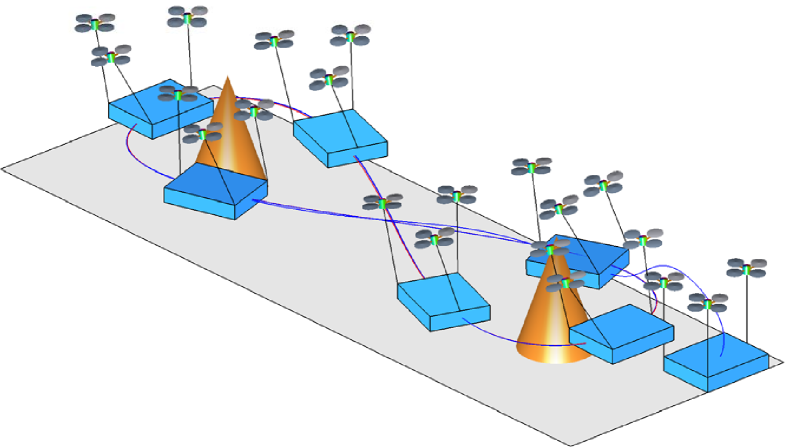
Figure 2: Snapshots of controlled maneuver (red:desired trajectory, blue:actual trajectory). A short animation illustrating this maneuver is available at http://youtu.be/nOWErfdzZLU.

The desired trajectory of the payload is chosen as

x0d(t)=[1.2sin(0.2πt), 4.2cos(0.1πt),0.5]Tm.subscript𝑥subscript0𝑑𝑡superscript1.20.2𝜋𝑡4.20.1𝜋𝑡0.5𝑇m\displaystyle x_{0_{d}}(t)=[1.2\sin(0.2\pi t),\,4.2\cos(0.1\pi t),\,-0.5]^{T}\,\mathrm{m}.

The desired attitude of the payload is chosen such that its first axis is tangent to the desired path, and the third axis is parallel to the direction of gravity, it is given by

R0d(t)=[x˙0dx˙0de^3x˙0de^3x˙0de3].subscript𝑅subscript0𝑑𝑡matrixsubscript˙𝑥subscript0𝑑normsubscript˙𝑥subscript0𝑑subscript^𝑒3subscript˙𝑥subscript0𝑑normsubscript^𝑒3subscript˙𝑥subscript0𝑑subscript𝑒3\displaystyle R_{0_{d}}(t)=\begin{bmatrix}\frac{\dot{x}_{0_{d}}}{\|\dot{x}_{0_{d}}\|}&\frac{\hat{e}_{3}\dot{x}_{0_{d}}}{\|\hat{e}_{3}\dot{x}_{0_{d}}\|}&e_{3}\end{bmatrix}.

Initial conditions are chosen as

x0(0)=[1, 4.8, 0]Tm,v0(0)=03×1m/s,formulae-sequencesubscript𝑥00superscript14.8 0𝑇msubscript𝑣00subscript031ms\displaystyle x_{0}(0)=[1,\,4.8,\,0]^{T}\,\mathrm{m},\quad v_{0}(0)=0_{3\times 1}\,\mathrm{m/s},
qi(0)=e3,ωi(0)=03×1,Ri(0)=I3×3,Ωi(0)=03×1.formulae-sequencesubscript𝑞𝑖0subscript𝑒3formulae-sequencesubscript𝜔𝑖0subscript031formulae-sequencesubscript𝑅𝑖0subscript𝐼33subscriptΩ𝑖0subscript031\displaystyle q_{i}(0)=e_{3},\;\omega_{i}(0)=0_{3\times 1},\;R_{i}(0)=I_{3\times 3},\;\Omega_{i}(0)=0_{3\times 1}.

The uncertainties are specified as
Δx0=[1, 3,2.5]T,ΔR0=[0.5, 0.1,1.5]T,formulae-sequencesubscriptΔsubscript𝑥0superscript132.5𝑇subscriptΔsubscript𝑅0superscript0.50.11.5𝑇\displaystyle\Delta_{x_{0}}=[1,\,3,\,-2.5]^{T},\quad\Delta_{R_{0}}=[-0.5,\,0.1,\,-1.5]^{T},
Δxi=[0.5,0.2, 0.3]T,ΔRi=[0.2, 0.3,0.7]T.formulae-sequencesubscriptΔsubscript𝑥𝑖superscript0.50.20.3𝑇subscriptΔsubscript𝑅𝑖superscript0.20.30.7𝑇\displaystyle\Delta_{x_{i}}=[0.5,\,-0.2,\,0.3]^{T},\quad\Delta_{R_{i}}=[0.2,\,0.3,\,-0.7]^{T}.

Refer to caption
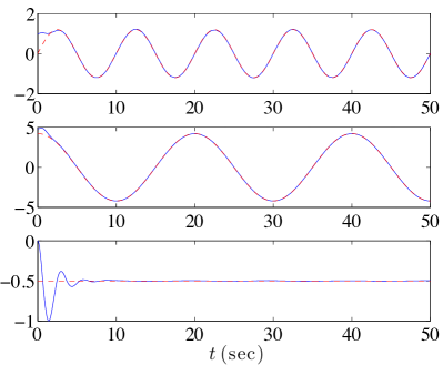
(a) Position of payload (x0subscript𝑥0x_{0}:blue, x0dsubscript𝑥subscript0𝑑x_{0_{d}}:red)
Refer to caption
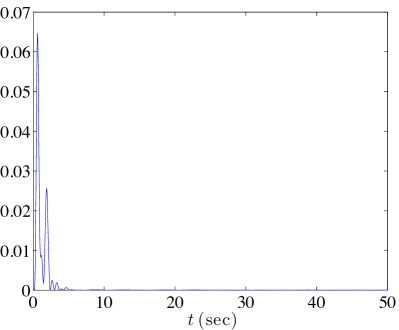
(b) Attitude tracking error of payload Ψ0=12R0R0d2subscriptΨ012superscriptnormsubscript𝑅0subscript𝑅subscript0𝑑2\Psi_{0}=\frac{1}{2}\|R_{0}-R_{0_{d}}\|^{2}

Refer to caption
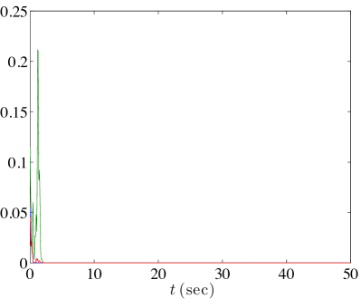
(c) Link direction error Ψqi=12qiqid2subscriptΨsubscript𝑞𝑖12superscriptnormsubscript𝑞𝑖subscript𝑞subscript𝑖𝑑2\Psi_{q_{i}}=\frac{1}{2}\|q_{i}-q_{i_{d}}\|^{2}
Refer to caption
(d) Attitude tracking error of quadrotors Ψi=12RiRid2subscriptΨ𝑖12superscriptnormsubscript𝑅𝑖subscript𝑅subscript𝑖𝑑2\Psi_{i}=\frac{1}{2}\|R_{i}-R_{i_{d}}\|^{2}

Refer to caption
(e) Tension at links
Refer to caption
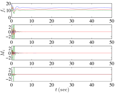
(f) Control input for quadrotors fi,Misubscript𝑓𝑖subscript𝑀𝑖f_{i},M_{i}
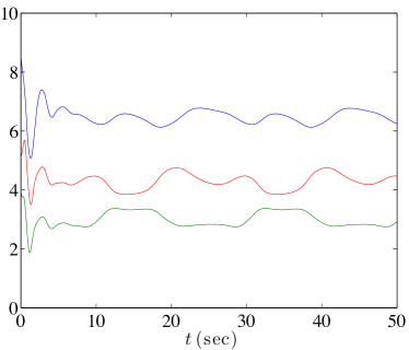
Figure 3: Simulation results for tracking errors and control inputs. (for figures (c)-(f): i=1𝑖1i=1:blue, i=2𝑖2i=2:green, i=3𝑖3i=3:red)

The corresponding simulation results are presented at Figures 2 and 3. Figure 2 illustrates the desired trajectory that is shaped like a figure-eight curve around two obstacles represented by cones, and the actual maneuver of the payload and quadrotors. Figure 3 shows tracking errors for the position and the attitude of the payload, tracking errors for the link directions and the attitude of quadrotors, as well as tension and control inputs. These illustrate excellent tracking performances of the proposed control system.

Error Dynamics

From (21) and (27), the dynamics of the position tracking error is given by

m0e¨x0subscript𝑚0subscript¨𝑒subscript𝑥0\displaystyle m_{0}\ddot{e}_{x_{0}} =m0(ge3x¨0d)+Δx0+i=1n(qiqiTμid+Δxi).absentsubscript𝑚0𝑔subscript𝑒3subscript¨𝑥subscript0𝑑subscriptΔsubscript𝑥0superscriptsubscript𝑖1𝑛subscript𝑞𝑖superscriptsubscript𝑞𝑖𝑇subscript𝜇subscript𝑖𝑑superscriptsubscriptΔsubscript𝑥𝑖parallel-to\displaystyle=m_{0}(ge_{3}-\ddot{x}_{0_{d}})+\Delta_{x_{0}}+\sum_{i=1}^{n}(q_{i}q_{i}^{T}\mu_{i_{d}}+\Delta_{x_{i}}^{\parallel}).

From (23) and (25), this can be rearranged as

e¨x0subscript¨𝑒subscript𝑥0\displaystyle\ddot{e}_{x_{0}} =ge3x¨0d+1m0Fd+Yx+1m0(Δx0+i=1nΔxi),absent𝑔subscript𝑒3subscript¨𝑥subscript0𝑑1subscript𝑚0subscript𝐹𝑑subscript𝑌𝑥1subscript𝑚0subscriptΔsubscript𝑥0superscriptsubscript𝑖1𝑛superscriptsubscriptΔsubscript𝑥𝑖parallel-to\displaystyle=ge_{3}-\ddot{x}_{0_{d}}+\frac{1}{m_{0}}F_{d}+Y_{x}+\frac{1}{m_{0}}(\Delta_{x_{0}}+\sum_{i=1}^{n}\Delta_{x_{i}}^{\parallel}),
=kx0ex0kx˙0e˙x0+1m0(Φx0θ~x0+i=1nΦxiθ~xi)+Yx,absentsubscript𝑘subscript𝑥0subscript𝑒subscript𝑥0subscript𝑘subscript˙𝑥0subscript˙𝑒subscript𝑥01subscript𝑚0subscriptΦsubscript𝑥0subscript~𝜃subscript𝑥0superscriptsubscript𝑖1𝑛superscriptsubscriptΦsubscript𝑥𝑖parallel-tosubscript~𝜃subscript𝑥𝑖subscript𝑌𝑥\displaystyle=-k_{x_{0}}e_{x_{0}}-k_{\dot{x}_{0}}\dot{e}_{x_{0}}+\frac{1}{m_{0}}(\Phi_{x_{0}}\tilde{\theta}_{x_{0}}+\sum_{i=1}^{n}\Phi_{x_{i}}^{\parallel}\tilde{\theta}_{x_{i}})+Y_{x}, (45)

where (13) is used and the estimation error is denoted by θ~xi=θxiθ¯xisubscript~𝜃subscript𝑥𝑖subscript𝜃subscript𝑥𝑖subscript¯𝜃subscript𝑥𝑖\tilde{\theta}_{x_{i}}=\theta_{x_{i}}-\bar{\theta}_{x_{i}}. At the above equation, the last term Yx3subscript𝑌𝑥superscript3Y_{x}\in\mathbb{R}^{3} represents the error caused by the difference between qisubscript𝑞𝑖q_{i} and qidsubscript𝑞subscript𝑖𝑑q_{i_{d}}, and it is given by

Yx=1m0i=1n(qiqiTI)μid.subscript𝑌𝑥1subscript𝑚0superscriptsubscript𝑖1𝑛subscript𝑞𝑖superscriptsubscript𝑞𝑖𝑇𝐼subscript𝜇subscript𝑖𝑑\displaystyle Y_{x}=\frac{1}{m_{0}}\sum_{i=1}^{n}(q_{i}q_{i}^{T}-I)\mu_{i_{d}}.

We have μid=qidqidTμidsubscript𝜇subscript𝑖𝑑subscript𝑞subscript𝑖𝑑superscriptsubscript𝑞subscript𝑖𝑑𝑇subscript𝜇subscript𝑖𝑑\mu_{i_{d}}=q_{i_{d}}q_{i_{d}}^{T}\mu_{i_{d}} from (28). Using this, the error term can be written in terms of eqisubscript𝑒subscript𝑞𝑖e_{q_{i}} as

Yxsubscript𝑌𝑥\displaystyle Y_{x} =1m0i=1n(qidTμid){(qiTqid)qiqid}absent1subscript𝑚0superscriptsubscript𝑖1𝑛superscriptsubscript𝑞subscript𝑖𝑑𝑇subscript𝜇subscript𝑖𝑑superscriptsubscript𝑞𝑖𝑇subscript𝑞subscript𝑖𝑑subscript𝑞𝑖subscript𝑞subscript𝑖𝑑\displaystyle=\frac{1}{m_{0}}\sum_{i=1}^{n}(q_{i_{d}}^{T}\mu_{i_{d}})\{(q_{i}^{T}q_{i_{d}})q_{i}-q_{i_{d}}\}
=1m0i=1n(qidTμid)q^ieqi.absent1subscript𝑚0superscriptsubscript𝑖1𝑛superscriptsubscript𝑞subscript𝑖𝑑𝑇subscript𝜇subscript𝑖𝑑subscript^𝑞𝑖subscript𝑒subscript𝑞𝑖\displaystyle=-\frac{1}{m_{0}}\sum_{i=1}^{n}(q_{i_{d}}^{T}\mu_{i_{d}})\hat{q}_{i}e_{q_{i}}.

Using (26), an upper bound of Yxsubscript𝑌𝑥Y_{x} can be obtained as

Yxnormsubscript𝑌𝑥\displaystyle\|Y_{x}\| 1m0i=1nμideqii=1nγ(Fd+Md)eqi,absent1subscript𝑚0superscriptsubscript𝑖1𝑛normsubscript𝜇subscript𝑖𝑑normsubscript𝑒subscript𝑞𝑖superscriptsubscript𝑖1𝑛𝛾normsubscript𝐹𝑑normsubscript𝑀𝑑normsubscript𝑒subscript𝑞𝑖\displaystyle\leq\frac{1}{m_{0}}\sum_{i=1}^{n}\|\mu_{i_{d}}\|\|e_{q_{i}}\|\leq\sum_{i=1}^{n}\gamma(\|F_{d}\|+\|M_{d}\|)\|e_{q_{i}}\|,

where γ=1m0λm[𝒫𝒫T]𝛾1subscript𝑚0subscript𝜆𝑚delimited-[]𝒫superscript𝒫𝑇\gamma=\frac{1}{m_{0}\sqrt{\lambda_{m}[\mathcal{P}\mathcal{P}^{T}]}}. From (23) and (24), this can be further bounded by

Yxnormsubscript𝑌𝑥absent\displaystyle\|Y_{x}\|\leq i=1n{β(kx0ex0+kx˙0e˙x0)\displaystyle\sum_{i=1}^{n}\{\beta(k_{x_{0}}\|e_{x_{0}}\|+k_{\dot{x}_{0}}\|\dot{e}_{x_{0}}\|)
+γ(kR0eR0+kΩ0eΩ0)+B}eqi,\displaystyle\quad+\gamma(k_{R_{0}}\|e_{R_{0}}\|+k_{\Omega_{0}}\|e_{\Omega_{0}}\|)+B\}\|e_{q_{i}}\|, (46)

where β=m0γ𝛽subscript𝑚0𝛾\beta=m_{0}\gamma, and the constant B𝐵B is determined by the given desired trajectories of the payload, the assumption (17) on the bounds of ΦΦ\Phi terms, and the adaptive law defined later that guarantee the boundedness of the estimated parameters θ¯¯𝜃\bar{\theta}. Throughout the remaining parts of the proof, any bound that can be obtained from x0d,R0dsubscript𝑥subscript0𝑑subscript𝑅subscript0𝑑x_{0_{d}},R_{0_{d}}, (17), or the adaptive law is denoted by B𝐵B for simplicity. In short, the position tracking error dynamics of the payload can be written as (45), where the error term is bounded by (46).

Similarly, we find the attitude tracking error dynamics for the payload as follows. Using (22), (24), and (27), the time-derivative of J0eΩ0subscript𝐽0subscript𝑒subscriptΩ0J_{0}e_{\Omega_{0}} can be written as

J0e˙Ω0subscript𝐽0subscript˙𝑒subscriptΩ0\displaystyle J_{0}\dot{e}_{\Omega_{0}} =(J0eΩ0+d)eΩ0kR0eR0kΩ0eΩ0absentsuperscriptsubscript𝐽0subscript𝑒subscriptΩ0𝑑subscript𝑒subscriptΩ0subscript𝑘subscript𝑅0subscript𝑒subscript𝑅0subscript𝑘subscriptΩ0subscript𝑒subscriptΩ0\displaystyle=(J_{0}e_{\Omega_{0}}+d)^{\wedge}e_{\Omega_{0}}-k_{R_{0}}e_{R_{0}}-k_{\Omega_{0}}e_{\Omega_{0}}
+ΦR0θ~R0+i=1nρ^iR0TΦR0θ~xi+YR,subscriptΦsubscript𝑅0subscript~𝜃subscript𝑅0superscriptsubscript𝑖1𝑛subscript^𝜌𝑖superscriptsubscript𝑅0𝑇superscriptsubscriptΦsubscript𝑅0parallel-tosubscript~𝜃subscript𝑥𝑖subscript𝑌𝑅\displaystyle\quad+\Phi_{R_{0}}\tilde{\theta}_{R_{0}}+\sum_{i=1}^{n}\hat{\rho}_{i}R_{0}^{T}\Phi_{R_{0}}^{\parallel}\tilde{\theta}_{x_{i}}+Y_{R}, (47)

where d=(2J0tr[J0]I)R0TR0dΩ0d3𝑑2subscript𝐽0trdelimited-[]subscript𝐽0𝐼superscriptsubscript𝑅0𝑇subscript𝑅subscript0𝑑subscriptΩsubscript0𝑑superscript3d=(2J_{0}-\mbox{tr}\!\left[J_{0}\right]I)R_{0}^{T}R_{0_{d}}\Omega_{0_{d}}\in\mathbb{R}^{3} [9] that is bounded, and Δ~R03subscript~Δsubscript𝑅0superscript3\tilde{\Delta}_{R_{0}}\in\mathbb{R}^{3} denotes the estimation error given by Δ~R0=ΔR0Δ^R0subscript~Δsubscript𝑅0subscriptΔsubscript𝑅0subscript^Δsubscript𝑅0\tilde{\Delta}_{R_{0}}=\Delta_{R_{0}}-\hat{\Delta}_{R_{0}}. The error term in the attitude dynamics of the payload, namely YR3subscript𝑌𝑅superscript3Y_{R}\in\mathbb{R}^{3} is given by

YRsubscript𝑌𝑅\displaystyle Y_{R} =i=1nρ^iR0T(qiqiTI)μid=i=1nρ^iR0T(qidTμid)q^ieqi.absentsuperscriptsubscript𝑖1𝑛subscript^𝜌𝑖superscriptsubscript𝑅0𝑇subscript𝑞𝑖superscriptsubscript𝑞𝑖𝑇𝐼subscript𝜇subscript𝑖𝑑superscriptsubscript𝑖1𝑛subscript^𝜌𝑖superscriptsubscript𝑅0𝑇superscriptsubscript𝑞subscript𝑖𝑑𝑇subscript𝜇subscript𝑖𝑑subscript^𝑞𝑖subscript𝑒subscript𝑞𝑖\displaystyle=\sum_{i=1}^{n}\hat{\rho}_{i}R_{0}^{T}(q_{i}q_{i}^{T}-I)\mu_{i_{d}}=-\sum_{i=1}^{n}\hat{\rho}_{i}R_{0}^{T}(q_{i_{d}}^{T}\mu_{i_{d}})\hat{q}_{i}e_{q_{i}}.

Similar with (46), an upper bound of YRsubscript𝑌𝑅Y_{R} can be obtained as

YRnormsubscript𝑌𝑅absent\displaystyle\|Y_{R}\|\leq i=1n{δi(kx0ex0+kx˙0e˙x0)\displaystyle\sum_{i=1}^{n}\{\delta_{i}(k_{x_{0}}\|e_{x_{0}}\|+k_{\dot{x}_{0}}\|\dot{e}_{x_{0}}\|)
+σi(kR0eR0+kΩ0eΩ0)+B}eqi,\displaystyle\quad+\sigma_{i}(k_{R_{0}}\|e_{R_{0}}\|+k_{\Omega_{0}}\|e_{\Omega_{0}}\|)+B\}\|e_{q_{i}}\|, (48)

where δi=m0ρ^iλm[𝒫𝒫T],σi=δim0formulae-sequencesubscript𝛿𝑖subscript𝑚0normsubscript^𝜌𝑖subscript𝜆𝑚delimited-[]𝒫superscript𝒫𝑇subscript𝜎𝑖subscript𝛿𝑖subscript𝑚0\delta_{i}=m_{0}\frac{\|\hat{\rho}_{i}\|}{\sqrt{\lambda_{m}[\mathcal{P}\mathcal{P}^{T}]}},\sigma_{i}=\frac{\delta_{i}}{m_{0}}\in\mathbb{R}.

Next, from (31), the time-derivative of the angular velocity error, projected on to the plane normal to qisubscript𝑞𝑖q_{i} is given as

q^i2e˙ωisuperscriptsubscript^𝑞𝑖2subscript˙𝑒subscript𝜔𝑖\displaystyle-\hat{q}_{i}^{2}\dot{e}_{\omega_{i}} =ω˙+(qωd)q˙+q^2ω˙dabsent˙𝜔𝑞subscript𝜔𝑑˙𝑞superscript^𝑞2subscript˙𝜔𝑑\displaystyle=\dot{\omega}+(q\cdot\omega_{d})\dot{q}+\hat{q}^{2}\dot{\omega}_{d}
=kqeqikωeωi1miliq^iΦxiθ~xi.absentsubscript𝑘𝑞subscript𝑒subscript𝑞𝑖subscript𝑘𝜔subscript𝑒subscript𝜔𝑖1subscript𝑚𝑖subscript𝑙𝑖subscript^𝑞𝑖superscriptsubscriptΦsubscript𝑥𝑖perpendicular-tosubscript~𝜃subscript𝑥𝑖\displaystyle=-k_{q}e_{q_{i}}-k_{\omega}e_{\omega_{i}}-\frac{1}{m_{i}l_{i}}\hat{q}_{i}\Phi_{x_{i}}^{\perp}\tilde{\theta}_{x_{i}}. (49)

In summary, the error dynamics of the simplified dynamic model are given by (45), (47) and (49).

Stability Proof

Define an attitude configuration error function ΨR0subscriptΨsubscript𝑅0\Psi_{R_{0}} for the payload as

ΨR0=12tr[IR0dTR0],subscriptΨsubscript𝑅012trdelimited-[]𝐼superscriptsubscript𝑅subscript0𝑑𝑇subscript𝑅0\displaystyle\Psi_{R_{0}}=\frac{1}{2}\mbox{tr}\!\left[I-R_{0_{d}}^{T}R_{0}\right],

which is positive-definite about R0=R0dsubscript𝑅0subscript𝑅subscript0𝑑R_{0}=R_{0_{d}}, and Ψ˙R0=eR0eΩ0subscript˙Ψsubscript𝑅0subscript𝑒subscript𝑅0subscript𝑒subscriptΩ0\dot{\Psi}_{R_{0}}=e_{R_{0}}\cdot e_{\Omega_{0}} [7, 9]. We also introduce a configuration error function ΨqisubscriptΨsubscript𝑞𝑖\Psi_{q_{i}} for each link that is positive-definite about qi=qidsubscript𝑞𝑖subscript𝑞subscript𝑖𝑑q_{i}=q_{i_{d}} as

Ψqi=1qiqid.subscriptΨsubscript𝑞𝑖1subscript𝑞𝑖subscript𝑞subscript𝑖𝑑\displaystyle\Psi_{q_{i}}=1-q_{i}\cdot q_{i_{d}}.

For positive constants exmax,ψR0,ψqisubscript𝑒subscript𝑥subscript𝜓subscript𝑅0subscript𝜓subscript𝑞𝑖e_{x_{\max}},\psi_{R_{0}},\psi_{q_{i}}, consider the following open domain containing the zero equilibrium of tracking error variables:

D={\displaystyle D=\{ (ex0,e˙x0,eR0,eΩ0,eqi,eωi,Δ~x0,Δ~R0,Δ~xi)subscript𝑒subscript𝑥0subscript˙𝑒subscript𝑥0subscript𝑒subscript𝑅0subscript𝑒subscriptΩ0subscript𝑒subscript𝑞𝑖subscript𝑒subscript𝜔𝑖subscript~Δsubscript𝑥0subscript~Δsubscript𝑅0subscript~Δsubscript𝑥𝑖\displaystyle(e_{x_{0}},\dot{e}_{x_{0}},e_{R_{0}},e_{\Omega_{0}},e_{q_{i}},e_{\omega_{i}},\tilde{\Delta}_{x_{0}},\tilde{\Delta}_{R_{0}},\tilde{\Delta}_{x_{i}})
(3)4×(3×3)n×(3)2×3n|\displaystyle\in(\mathbb{R}^{3})^{4}\times(\mathbb{R}^{3}\times\mathbb{R}^{3})^{n}\times(\mathbb{R}^{3})^{2}\times\mathbb{R}^{3n}\,|\,
ex0<exmax,ΨR0<ψR0<1,Ψqi<ψqi<1}.\displaystyle\|e_{x_{0}}\|<e_{x_{\max}},\,\Psi_{R_{0}}<\psi_{R_{0}}<1,\,\Psi_{q_{i}}<\psi_{q_{i}}<1\}. (50)

In this domain, we have eR0=ΨR0(2ΨR0)ψR0(2ψR0)α0<1normsubscript𝑒subscript𝑅0subscriptΨsubscript𝑅02subscriptΨsubscript𝑅0subscript𝜓subscript𝑅02subscript𝜓subscript𝑅0subscript𝛼01\|e_{R_{0}}\|=\sqrt{\Psi_{R_{0}}(2-\Psi_{R_{0}})}\leq\sqrt{\psi_{R_{0}}(2-\psi_{R_{0}})}\triangleq\alpha_{0}<1, and eqi=Ψqi(2Ψqi)ψqi(2ψqi)αi<1normsubscript𝑒subscript𝑞𝑖subscriptΨsubscript𝑞𝑖2subscriptΨsubscript𝑞𝑖subscript𝜓subscript𝑞𝑖2subscript𝜓subscript𝑞𝑖subscript𝛼𝑖1\|e_{q_{i}}\|=\sqrt{\Psi_{q_{i}}(2-\Psi_{q_{i}})}\leq\sqrt{\psi_{q_{i}}(2-\psi_{q_{i}})}\triangleq\alpha_{i}<1. It is assumed that ψqisubscript𝜓subscript𝑞𝑖\psi_{q_{i}} is sufficiently small such that nαiβ<1𝑛subscript𝛼𝑖𝛽1n\alpha_{i}\beta<1.

We can show that the configuration error functions are quadratic with respect to the error vectors in the sense that

12eR02ΨR012ψR0eR02,12superscriptnormsubscript𝑒subscript𝑅02subscriptΨsubscript𝑅012subscript𝜓subscript𝑅0superscriptnormsubscript𝑒subscript𝑅02\displaystyle\frac{1}{2}\|e_{R_{0}}\|^{2}\leq\Psi_{R_{0}}\leq\frac{1}{2-\psi_{R_{0}}}\|e_{R_{0}}\|^{2},
12eqi2Ψqi12ψqieqi2,12superscriptnormsubscript𝑒subscript𝑞𝑖2subscriptΨsubscript𝑞𝑖12subscript𝜓subscript𝑞𝑖superscriptnormsubscript𝑒subscript𝑞𝑖2\displaystyle\frac{1}{2}\|e_{q_{i}}\|^{2}\leq\Psi_{q_{i}}\leq\frac{1}{2-\psi_{q_{i}}}\|e_{q_{i}}\|^{2},

where the upper bounds are satisfied only in the domain D𝐷D.

Define

𝒱0subscript𝒱0\displaystyle\mathcal{V}_{0} =12e˙x02+12kx0ex02+cxex0e˙x0absent12superscriptnormsubscript˙𝑒subscript𝑥0212subscript𝑘subscript𝑥0superscriptnormsubscript𝑒subscript𝑥02subscript𝑐𝑥subscript𝑒subscript𝑥0subscript˙𝑒subscript𝑥0\displaystyle=\frac{1}{2}\|\dot{e}_{x_{0}}\|^{2}+\frac{1}{2}k_{x_{0}}\|e_{x_{0}}\|^{2}+c_{x}e_{x_{0}}\cdot\dot{e}_{x_{0}}
+12eΩ0J0Ω0+kR0ΨR0+cReR0J0eΩ012subscript𝑒subscriptΩ0subscript𝐽0subscriptΩ0subscript𝑘subscript𝑅0subscriptΨsubscript𝑅0subscript𝑐𝑅subscript𝑒subscript𝑅0subscript𝐽0subscript𝑒subscriptΩ0\displaystyle\quad+\frac{1}{2}e_{\Omega_{0}}\cdot J_{0}\Omega_{0}+k_{R_{0}}\Psi_{R_{0}}+c_{R}e_{R_{0}}\cdot J_{0}e_{\Omega_{0}}
+i=1n12eωi2+kqΨqi+cqeqieωi,superscriptsubscript𝑖1𝑛12superscriptnormsubscript𝑒subscript𝜔𝑖2subscript𝑘𝑞subscriptΨsubscript𝑞𝑖subscript𝑐𝑞subscript𝑒subscript𝑞𝑖subscript𝑒subscript𝜔𝑖\displaystyle\quad+\sum_{i=1}^{n}\frac{1}{2}\|e_{\omega_{i}}\|^{2}+k_{q}\Psi_{q_{i}}+c_{q}e_{q_{i}}\cdot e_{\omega_{i}},

where cx,cR,cqsubscript𝑐𝑥subscript𝑐𝑅subscript𝑐𝑞c_{x},c_{R},c_{q} are positive constants. This is composed of tracking error variables only, and we define another function for the estimation errors of the adaptive laws as

𝒱asubscript𝒱𝑎\displaystyle\mathcal{V}_{a} =12hx0θ~x02+12hR0θ~R02+i=1n12hxiθ~xi2.absent12subscriptsubscript𝑥0superscriptnormsubscript~𝜃subscript𝑥0212subscriptsubscript𝑅0superscriptnormsubscript~𝜃subscript𝑅02superscriptsubscript𝑖1𝑛12subscriptsubscript𝑥𝑖superscriptnormsubscript~𝜃subscript𝑥𝑖2\displaystyle=\frac{1}{2h_{x_{0}}}\|\tilde{\theta}_{x_{0}}\|^{2}+\frac{1}{2h_{R_{0}}}\|\tilde{\theta}_{R_{0}}\|^{2}+\sum_{i=1}^{n}\frac{1}{2h_{x_{i}}}\|\tilde{\theta}_{x_{i}}\|^{2}.

The Lyapunov function for the complete simplified dynamic model is chosen as 𝒱=𝒱0+𝒱a𝒱subscript𝒱0subscript𝒱𝑎\mathcal{V}=\mathcal{V}_{0}+\mathcal{V}_{a}.

Let zx0=[ex0,e˙x0]Tsubscript𝑧subscript𝑥0superscriptnormsubscript𝑒subscript𝑥0normsubscript˙𝑒subscript𝑥0𝑇z_{x_{0}}=[\|e_{x_{0}}\|,\|\dot{e}_{x_{0}}\|]^{T}, zR0=[eR0,eΩ0]Tsubscript𝑧subscript𝑅0superscriptnormsubscript𝑒subscript𝑅0normsubscript𝑒subscriptΩ0𝑇z_{R_{0}}=[\|e_{R_{0}}\|,\|e_{\Omega_{0}}\|]^{T}, zqi=[eqi,eωi]T2subscript𝑧subscript𝑞𝑖superscriptnormsubscript𝑒subscript𝑞𝑖normsubscript𝑒subscript𝜔𝑖𝑇superscript2z_{q_{i}}=[\|e_{q_{i}}\|,\|e_{\omega_{i}}\|]^{T}\in\mathbb{R}^{2}. The first part of the Lyapunov function 𝒱0subscript𝒱0\mathcal{V}_{0} satisfies

zx0Tsuperscriptsubscript𝑧subscript𝑥0𝑇\displaystyle z_{x_{0}}^{T} P¯x0zx0+zR0TP¯R0zR0+i=1nzqiTP¯qizqi𝒱0subscript¯𝑃subscript𝑥0subscript𝑧subscript𝑥0superscriptsubscript𝑧subscript𝑅0𝑇subscript¯𝑃subscript𝑅0subscript𝑧subscript𝑅0superscriptsubscript𝑖1𝑛superscriptsubscript𝑧subscript𝑞𝑖𝑇subscript¯𝑃subscript𝑞𝑖subscript𝑧subscript𝑞𝑖subscript𝒱0\displaystyle\underline{P}_{x_{0}}z_{x_{0}}+z_{R_{0}}^{T}\underline{P}_{R_{0}}z_{R_{0}}+\sum_{i=1}^{n}z_{q_{i}}^{T}\underline{P}_{q_{i}}z_{q_{i}}\leq\mathcal{V}_{0}
zx0TP¯x0zx0+zR0TP¯R0zR0+i=1nzqiTP¯qizqi,absentsuperscriptsubscript𝑧subscript𝑥0𝑇subscript¯𝑃subscript𝑥0subscript𝑧subscript𝑥0superscriptsubscript𝑧subscript𝑅0𝑇subscript¯𝑃subscript𝑅0subscript𝑧subscript𝑅0superscriptsubscript𝑖1𝑛superscriptsubscript𝑧subscript𝑞𝑖𝑇subscript¯𝑃subscript𝑞𝑖subscript𝑧subscript𝑞𝑖\displaystyle\leq z_{x_{0}}^{T}\overline{P}_{x_{0}}z_{x_{0}}+z_{R_{0}}^{T}\overline{P}_{R_{0}}z_{R_{0}}+\sum_{i=1}^{n}z_{q_{i}}^{T}\overline{P}_{q_{i}}z_{q_{i}},

where the matrices P¯x0,P¯R0,P¯qi,P¯x0,P¯R0,P¯qi2×2subscript¯𝑃subscript𝑥0subscript¯𝑃subscript𝑅0subscript¯𝑃subscript𝑞𝑖subscript¯𝑃subscript𝑥0subscript¯𝑃subscript𝑅0subscript¯𝑃subscript𝑞𝑖superscript22\underline{P}_{x_{0}},\underline{P}_{R_{0}},\underline{P}_{q_{i}},\underline{P}_{x_{0}},\underline{P}_{R_{0}},\underline{P}_{q_{i}}\in\mathbb{R}^{2\times 2} are given by

P¯x0subscript¯𝑃subscript𝑥0\displaystyle\underline{P}_{x_{0}} =12[kx0cxcx1],absent12matrixsubscript𝑘subscript𝑥0subscript𝑐𝑥subscript𝑐𝑥1\displaystyle=\frac{1}{2}\begin{bmatrix}k_{x_{0}}&-c_{x}\\ -c_{x}&1\end{bmatrix}, P¯x0subscript¯𝑃subscript𝑥0\displaystyle\;\overline{P}_{x_{0}} =12[kx0cxcx1],absent12matrixsubscript𝑘subscript𝑥0subscript𝑐𝑥subscript𝑐𝑥1\displaystyle=\frac{1}{2}\begin{bmatrix}k_{x_{0}}&c_{x}\\ c_{x}&1\end{bmatrix},
P¯R0subscript¯𝑃subscript𝑅0\displaystyle\underline{P}_{R_{0}} =12[2kR0cRλ¯cRλ¯λ¯],absent12matrix2subscript𝑘subscript𝑅0subscript𝑐𝑅¯𝜆subscript𝑐𝑅¯𝜆¯𝜆\displaystyle=\frac{1}{2}\begin{bmatrix}2k_{R_{0}}&-c_{R}\overline{\lambda}\\ -c_{R}\overline{\lambda}&\underline{\lambda}\end{bmatrix}, P¯R0subscript¯𝑃subscript𝑅0\displaystyle\overline{P}_{R_{0}} =12[2kR02ψR0cRλ¯cRλ¯λ¯],absent12matrix2subscript𝑘subscript𝑅02subscript𝜓subscript𝑅0subscript𝑐𝑅¯𝜆subscript𝑐𝑅¯𝜆¯𝜆\displaystyle=\frac{1}{2}\begin{bmatrix}\frac{2k_{R_{0}}}{2-\psi_{R_{0}}}&c_{R}\overline{\lambda}\\ c_{R}\overline{\lambda}&\overline{\lambda}\end{bmatrix},
P¯qisubscript¯𝑃subscript𝑞𝑖\displaystyle\underline{P}_{q_{i}} =12[2kqcqcq1],absent12matrix2subscript𝑘𝑞subscript𝑐𝑞subscript𝑐𝑞1\displaystyle=\frac{1}{2}\begin{bmatrix}2k_{q}&-c_{q}\\ -c_{q}&1\end{bmatrix}, P¯qisubscript¯𝑃subscript𝑞𝑖\displaystyle\overline{P}_{q_{i}} =12[2kq2ψqicqcq1],absent12matrix2subscript𝑘𝑞2subscript𝜓subscript𝑞𝑖subscript𝑐𝑞subscript𝑐𝑞1\displaystyle=\frac{1}{2}\begin{bmatrix}\frac{2k_{q}}{2-\psi_{q_{i}}}&c_{q}\\ c_{q}&1\end{bmatrix},

where λ¯=λm[J0]¯𝜆subscript𝜆𝑚delimited-[]subscript𝐽0\underline{\lambda}=\lambda_{m}[J_{0}] and λ¯=λM[J0]¯𝜆subscript𝜆𝑀delimited-[]subscript𝐽0\overline{\lambda}=\lambda_{M}[J_{0}]. If the constants cx,cR0,cqsubscript𝑐𝑥subscript𝑐subscript𝑅0subscript𝑐𝑞c_{x},c_{R_{0}},c_{q} are sufficiently small, all of the above matrices are positive-definite. As the second part of the Lyapunov function 𝒱asubscript𝒱𝑎\mathcal{V}_{a} is already given as a quadratic form, it is straightforward to see that the complete Lyapunov function 𝒱𝒱\mathcal{V} is positive-definite and decrescent.

The time-derivative of the Lyapunov function along the error dynamics (45), (47), and (49) is given by

𝒱˙˙𝒱\displaystyle\dot{\mathcal{V}} =(kx˙0cx)e˙x02cxkx0ex02cxkx˙0ex0e˙x0absentsubscript𝑘subscript˙𝑥0subscript𝑐𝑥superscriptnormsubscript˙𝑒subscript𝑥02subscript𝑐𝑥subscript𝑘subscript𝑥0superscriptnormsubscript𝑒subscript𝑥02subscript𝑐𝑥subscript𝑘subscript˙𝑥0subscript𝑒subscript𝑥0subscript˙𝑒subscript𝑥0\displaystyle=-(k_{\dot{x}_{0}}-c_{x})\|\dot{e}_{x_{0}}\|^{2}-c_{x}k_{x_{0}}\|e_{x_{0}}\|^{2}-c_{x}k_{\dot{x}_{0}}e_{x_{0}}\cdot\dot{e}_{x_{0}}
+(cxex0+e˙x0)YxkΩ0eΩ02+cRe˙RJ0eΩ0subscript𝑐𝑥subscript𝑒subscript𝑥0subscript˙𝑒subscript𝑥0subscript𝑌𝑥subscript𝑘subscriptΩ0superscriptnormsubscript𝑒subscriptΩ02subscript𝑐𝑅subscript˙𝑒𝑅subscript𝐽0subscript𝑒subscriptΩ0\displaystyle\quad+(c_{x}e_{x_{0}}+\dot{e}_{x_{0}})\cdot Y_{x}-k_{\Omega_{0}}\|e_{\Omega_{0}}\|^{2}+c_{R}\dot{e}_{R}\cdot J_{0}e_{\Omega_{0}}
cRkR0eR02+cReR0((J0eΩ0+d)eΩ0kΩ0eΩ0)subscript𝑐𝑅subscript𝑘subscript𝑅0superscriptnormsubscript𝑒subscript𝑅02subscript𝑐𝑅subscript𝑒subscript𝑅0superscriptsubscript𝐽0subscript𝑒subscriptΩ0𝑑subscript𝑒subscriptΩ0subscript𝑘subscriptΩ0subscript𝑒subscriptΩ0\displaystyle\quad-c_{R}k_{R_{0}}\|e_{R_{0}}\|^{2}+c_{R}e_{R_{0}}\cdot((J_{0}e_{\Omega_{0}}+d)^{\wedge}e_{\Omega_{0}}-k_{\Omega_{0}}e_{\Omega_{0}})
+(eΩ0+cReR0)YRsubscript𝑒subscriptΩ0subscript𝑐𝑅subscript𝑒subscript𝑅0subscript𝑌𝑅\displaystyle\quad+(e_{\Omega_{0}}+c_{R}e_{R_{0}})\cdot Y_{R}
+i=1n(kωcq)eωi2cqkqeqi2cqkωeqieωisuperscriptsubscript𝑖1𝑛subscript𝑘𝜔subscript𝑐𝑞superscriptnormsubscript𝑒subscript𝜔𝑖2subscript𝑐𝑞subscript𝑘𝑞superscriptnormsubscript𝑒subscript𝑞𝑖2subscript𝑐𝑞subscript𝑘𝜔subscript𝑒subscript𝑞𝑖subscript𝑒subscript𝜔𝑖\displaystyle\quad+\sum_{i=1}^{n}-(k_{\omega}-c_{q})\|e_{\omega_{i}}\|^{2}-c_{q}k_{q}\|e_{q_{i}}\|^{2}-c_{q}k_{\omega}e_{q_{i}}\cdot e_{\omega_{i}}
+1m0(e˙x0+cxex0)(Φx0θ~x0+i=1nΦxiθ~xi)1subscript𝑚0subscript˙𝑒subscript𝑥0subscript𝑐𝑥subscript𝑒subscript𝑥0subscriptΦsubscript𝑥0subscript~𝜃subscript𝑥0superscriptsubscript𝑖1𝑛superscriptsubscriptΦsubscript𝑥𝑖parallel-tosubscript~𝜃subscript𝑥𝑖\displaystyle\quad+\frac{1}{m_{0}}(\dot{e}_{x_{0}}+c_{x}e_{x_{0}})\cdot(\Phi_{x_{0}}\tilde{\theta}_{x_{0}}+\sum_{i=1}^{n}\Phi_{x_{i}}^{\parallel}\tilde{\theta}_{x_{i}})
+(eΩ0+cReR0)(ΦR0θ~R0+i=1nρ^iR0TΦxiθ~xi)subscript𝑒subscriptΩ0subscript𝑐𝑅subscript𝑒subscript𝑅0subscriptΦsubscript𝑅0subscript~𝜃subscript𝑅0superscriptsubscript𝑖1𝑛subscript^𝜌𝑖superscriptsubscript𝑅0𝑇superscriptsubscriptΦsubscript𝑥𝑖parallel-tosubscript~𝜃subscript𝑥𝑖\displaystyle\quad+(e_{\Omega_{0}}+c_{R}e_{R_{0}})\cdot(\Phi_{R_{0}}\tilde{\theta}_{R_{0}}+\sum_{i=1}^{n}\hat{\rho}_{i}R_{0}^{T}\Phi_{x_{i}}^{\parallel}\tilde{\theta}_{x_{i}})
(i=1n(eωi+cqeqi)q^imiliΦxiθ~xi)1hx0θ~x0θ¯˙x0superscriptsubscript𝑖1𝑛subscript𝑒subscript𝜔𝑖subscript𝑐𝑞subscript𝑒subscript𝑞𝑖subscript^𝑞𝑖subscript𝑚𝑖subscript𝑙𝑖superscriptsubscriptΦsubscript𝑥𝑖perpendicular-tosubscript~𝜃subscript𝑥𝑖1subscriptsubscript𝑥0subscript~𝜃subscript𝑥0subscript˙¯𝜃subscript𝑥0\displaystyle\quad-\left(\sum_{i=1}^{n}(e_{\omega_{i}}+c_{q}e_{q_{i}})\cdot\frac{\hat{q}_{i}}{m_{i}l_{i}}\Phi_{x_{i}}^{\perp}\tilde{\theta}_{x_{i}}\right)-\frac{1}{h_{x_{0}}}\tilde{\theta}_{x_{0}}\cdot\dot{\bar{\theta}}_{x_{0}}
1hR0θ~R0θ¯˙R0i=1n1hxiθ~xiθ¯˙xi.1subscriptsubscript𝑅0subscript~𝜃subscript𝑅0subscript˙¯𝜃subscript𝑅0superscriptsubscript𝑖1𝑛1subscriptsubscript𝑥𝑖subscript~𝜃subscript𝑥𝑖subscript˙¯𝜃subscript𝑥𝑖\displaystyle\quad-\frac{1}{h_{R_{0}}}\tilde{\theta}_{R_{0}}\cdot\dot{\bar{\theta}}_{R_{0}}-\sum_{i=1}^{n}\frac{1}{h_{x_{i}}}\tilde{\theta}_{x_{i}}\cdot\dot{\bar{\theta}}_{x_{i}}. (51)

In the above equation, the expressions at the last four lines depending on the estimate error can be rearranged by using the adaptive laws, (34)-(39) as

θ~x0(yx0Pr(θ¯x0,yx0))+θ~R0(yR0Pr(θ¯R0,yR0))subscript~𝜃subscript𝑥0subscript𝑦subscript𝑥0Prsubscript¯𝜃subscript𝑥0subscript𝑦subscript𝑥0subscript~𝜃subscript𝑅0subscript𝑦subscript𝑅0Prsubscript¯𝜃subscript𝑅0subscript𝑦subscript𝑅0\displaystyle\tilde{\theta}_{x_{0}}\cdot(y_{x_{0}}-\mathrm{Pr}(\bar{\theta}_{x_{0}},y_{x_{0}}))+\tilde{\theta}_{R_{0}}\cdot(y_{R_{0}}-\mathrm{Pr}(\bar{\theta}_{R_{0}},y_{R_{0}}))
+i=1nθ~xi(yxiPr(θ¯xi,yxi)).superscriptsubscript𝑖1𝑛subscript~𝜃subscript𝑥𝑖subscript𝑦subscript𝑥𝑖Prsubscript¯𝜃subscript𝑥𝑖subscript𝑦subscript𝑥𝑖\displaystyle\quad+\sum_{i=1}^{n}\tilde{\theta}_{x_{i}}\cdot(y_{x_{i}}-\mathrm{Pr}(\bar{\theta}_{x_{i}},y_{x_{i}})).

From the definition of the projection map, the above expressions vanish for the first case of (33). For the second case,

(θθ¯)(yPr(θ¯,y))𝜃¯𝜃𝑦Pr¯𝜃𝑦\displaystyle(\theta-\bar{\theta})\cdot(y-\mathrm{Pr}(\bar{\theta},y)) =1θ¯2(θθ¯)θ¯θ¯Tyabsent1superscriptnorm¯𝜃2𝜃¯𝜃¯𝜃superscript¯𝜃𝑇𝑦\displaystyle=\frac{1}{\left\|\bar{\theta}\right\|^{2}}(\theta-\bar{\theta})\cdot\bar{\theta}\bar{\theta}^{T}y
=1θ¯2(θ¯Tθθ¯Tθ¯)(θ¯Ty)0.absent1superscriptnorm¯𝜃2superscript¯𝜃𝑇𝜃superscript¯𝜃𝑇¯𝜃superscript¯𝜃𝑇𝑦0\displaystyle=\frac{1}{\left\|\bar{\theta}\right\|^{2}}(\bar{\theta}^{T}\theta-\bar{\theta}^{T}\bar{\theta})(\bar{\theta}^{T}y)\leq 0.

for each estimated parameter. The last inequality is due to (θ¯Tθθ¯Tθ¯)0superscript¯𝜃𝑇𝜃superscript¯𝜃𝑇¯𝜃0(\bar{\theta}^{T}\theta-\bar{\theta}^{T}\bar{\theta})\leq 0 and (θ¯Ty)>0superscript¯𝜃𝑇𝑦0(\bar{\theta}^{T}y)>0 obtained by (18) and (33).

An upper bound of the remaining expressions of 𝒱˙˙𝒱\dot{\mathcal{V}} at (51) can be obtained as follows. Since eR01normsubscript𝑒subscript𝑅01\|e_{R_{0}}\|\leq 1, e˙R0eΩ0normsubscript˙𝑒subscript𝑅0normsubscript𝑒subscriptΩ0\|\dot{e}_{R_{0}}\|\leq\|e_{\Omega_{0}}\| and dBnorm𝑑𝐵\|d\|\leq B,

𝒱˙˙𝒱\displaystyle\dot{\mathcal{V}} (kx˙0cx)e˙x02cxkx0ex02cxkx˙0ex0e˙x0absentsubscript𝑘subscript˙𝑥0subscript𝑐𝑥superscriptnormsubscript˙𝑒subscript𝑥02subscript𝑐𝑥subscript𝑘subscript𝑥0superscriptnormsubscript𝑒subscript𝑥02subscript𝑐𝑥subscript𝑘subscript˙𝑥0subscript𝑒subscript𝑥0subscript˙𝑒subscript𝑥0\displaystyle\leq-(k_{\dot{x}_{0}}-c_{x})\|\dot{e}_{x_{0}}\|^{2}-c_{x}k_{x_{0}}\|e_{x_{0}}\|^{2}-c_{x}k_{\dot{x}_{0}}e_{x_{0}}\cdot\dot{e}_{x_{0}}
+(cxex0+e˙x0)Yx(kΩ02cRλ¯)eΩ02subscript𝑐𝑥subscript𝑒subscript𝑥0subscript˙𝑒subscript𝑥0subscript𝑌𝑥subscript𝑘subscriptΩ02subscript𝑐𝑅¯𝜆superscriptnormsubscript𝑒subscriptΩ02\displaystyle\quad+(c_{x}e_{x_{0}}+\dot{e}_{x_{0}})\cdot Y_{x}-(k_{\Omega_{0}}-2c_{R}\overline{\lambda})\|e_{\Omega_{0}}\|^{2}
cRkR0eR02+cR(kΩ0+B)eR0eΩ0subscript𝑐𝑅subscript𝑘subscript𝑅0superscriptnormsubscript𝑒subscript𝑅02subscript𝑐𝑅subscript𝑘subscriptΩ0𝐵normsubscript𝑒subscript𝑅0normsubscript𝑒subscriptΩ0\displaystyle\quad-c_{R}k_{R_{0}}\|e_{R_{0}}\|^{2}+c_{R}(k_{\Omega_{0}}+B)\|e_{R_{0}}\|\|e_{\Omega_{0}}\|
+(eΩ0+cReR0)YRsubscript𝑒subscriptΩ0subscript𝑐𝑅subscript𝑒subscript𝑅0subscript𝑌𝑅\displaystyle\quad+(e_{\Omega_{0}}+c_{R}e_{R_{0}})\cdot Y_{R}
+i=1n(kωcq)eωi2cqkqeqi2cqkωeqieωi.superscriptsubscript𝑖1𝑛subscript𝑘𝜔subscript𝑐𝑞superscriptnormsubscript𝑒subscript𝜔𝑖2subscript𝑐𝑞subscript𝑘𝑞superscriptnormsubscript𝑒subscript𝑞𝑖2subscript𝑐𝑞subscript𝑘𝜔subscript𝑒subscript𝑞𝑖subscript𝑒subscript𝜔𝑖\displaystyle\quad+\sum_{i=1}^{n}-(k_{\omega}-c_{q})\|e_{\omega_{i}}\|^{2}-c_{q}k_{q}\|e_{q_{i}}\|^{2}-c_{q}k_{\omega}e_{q_{i}}\cdot e_{\omega_{i}}. (52)

From (46), an upper bound of the fourth term of the right-hand side is given by

\displaystyle\| (cxex0+e˙x0)Yxconditionalsubscript𝑐𝑥subscript𝑒subscript𝑥0subscript˙𝑒subscript𝑥0subscript𝑌𝑥\displaystyle(c_{x}e_{x_{0}}+\dot{e}_{x_{0}})\cdot Y_{x}\|\leq
i=1nαiβ(cxkx0ex02+cxkx˙0ex0e˙x0+kx˙0e˙x02)superscriptsubscript𝑖1𝑛subscript𝛼𝑖𝛽subscript𝑐𝑥subscript𝑘subscript𝑥0superscriptnormsubscript𝑒subscript𝑥02subscript𝑐𝑥subscript𝑘subscript˙𝑥0normsubscript𝑒subscript𝑥0normsubscript˙𝑒subscript𝑥0subscript𝑘subscript˙𝑥0superscriptnormsubscript˙𝑒subscript𝑥02\displaystyle\sum_{i=1}^{n}\alpha_{i}\beta(c_{x}k_{x_{0}}\|e_{x_{0}}\|^{2}+c_{x}k_{\dot{x}_{0}}\|e_{x_{0}}\|\|\dot{e}_{x_{0}}\|+k_{\dot{x}_{0}}\|\dot{e}_{x_{0}}\|^{2})
+{cxBex+(βkx0exmax+B)e˙x0}eqisubscript𝑐𝑥𝐵normsubscript𝑒𝑥𝛽subscript𝑘subscript𝑥0subscript𝑒subscript𝑥𝐵normsubscript˙𝑒subscript𝑥0normsubscript𝑒subscript𝑞𝑖\displaystyle+\{c_{x}B\|e_{x}\|+(\beta k_{x_{0}}e_{x_{\max}}+B)\|\dot{e}_{x_{0}}\|\}\|e_{q_{i}}\|
+αiγ(cxex0+e˙x0)(kR0eR0+kΩ0eΩ0).subscript𝛼𝑖𝛾subscript𝑐𝑥normsubscript𝑒subscript𝑥0normsubscript˙𝑒subscript𝑥0subscript𝑘subscript𝑅0normsubscript𝑒subscript𝑅0subscript𝑘subscriptΩ0normsubscript𝑒subscriptΩ0\displaystyle+\alpha_{i}\gamma(c_{x}\|e_{x_{0}}\|+\|\dot{e}_{x_{0}}\|)(k_{R_{0}}\|e_{R_{0}}\|+k_{\Omega_{0}}\|e_{\Omega_{0}}\|). (53)

Similarly, using (48),

\displaystyle\| (cReR0+eΩ0)YRconditionalsubscript𝑐𝑅subscript𝑒subscript𝑅0subscript𝑒subscriptΩ0subscript𝑌𝑅\displaystyle(c_{R}e_{R_{0}}+e_{\Omega_{0}})\cdot Y_{R}\|\leq
i=1nαiσi(cRkR0eR02+cRkΩ0eR0eΩ0+kΩ0eΩ02)superscriptsubscript𝑖1𝑛subscript𝛼𝑖subscript𝜎𝑖subscript𝑐𝑅subscript𝑘subscript𝑅0superscriptnormsubscript𝑒subscript𝑅02subscript𝑐𝑅subscript𝑘subscriptΩ0normsubscript𝑒subscript𝑅0normsubscript𝑒subscriptΩ0subscript𝑘subscriptΩ0superscriptnormsubscript𝑒subscriptΩ02\displaystyle\sum_{i=1}^{n}\alpha_{i}\sigma_{i}(c_{R}k_{R_{0}}\|e_{R_{0}}\|^{2}+c_{R}k_{\Omega_{0}}\|e_{R_{0}}\|\|e_{\Omega_{0}}\|+k_{\Omega_{0}}\|e_{\Omega_{0}}\|^{2})
+{cRBeR0+(α0σikR0+B)eΩ0}eqisubscript𝑐𝑅𝐵normsubscript𝑒subscript𝑅0subscript𝛼0subscript𝜎𝑖subscript𝑘subscript𝑅0𝐵normsubscript𝑒subscriptΩ0normsubscript𝑒subscript𝑞𝑖\displaystyle+\{c_{R}B\|e_{R_{0}}\|+(\alpha_{0}\sigma_{i}k_{R_{0}}+B)\|e_{\Omega_{0}}\|\}\|e_{q_{i}}\|
+αiδi(cReR0+eΩ0)(kx0ex0+kx˙0e˙x0).subscript𝛼𝑖subscript𝛿𝑖subscript𝑐𝑅normsubscript𝑒subscript𝑅0normsubscript𝑒subscriptΩ0subscript𝑘subscript𝑥0normsubscript𝑒subscript𝑥0subscript𝑘subscript˙𝑥0normsubscript˙𝑒subscript𝑥0\displaystyle+\alpha_{i}\delta_{i}(c_{R}\|e_{R_{0}}\|+\|e_{\Omega_{0}}\|)(k_{x_{0}}\|e_{x_{0}}\|+k_{\dot{x}_{0}}\|\dot{e}_{x_{0}}\|). (54)

Substituting these into (52) and rearranging,

𝒱˙i=1nziTWizi,˙𝒱superscriptsubscript𝑖1𝑛superscriptsubscript𝑧𝑖𝑇subscript𝑊𝑖subscript𝑧𝑖\displaystyle\dot{\mathcal{V}}\leq\sum_{i=1}^{n}-z_{i}^{T}W_{i}z_{i}, (55)

where zi=[zx0,zR0,zqi]T3subscript𝑧𝑖superscriptnormsubscript𝑧subscript𝑥0normsubscript𝑧subscript𝑅0normsubscript𝑧subscript𝑞𝑖𝑇superscript3z_{i}=[\|z_{x_{0}}\|,\,\|z_{R_{0}}\|,\,\ \|z_{q_{i}}\|]^{T}\in\mathbb{R}^{3}, and the matrix Wi3×3subscript𝑊𝑖superscript33W_{i}\in\mathbb{R}^{3\times 3} is defined as

Wi=[λm[Wxi]12WxRi12Wxqi12WxRiλm[WRi]12WRqi12Wxqi12WRqiλm[Wqi]],subscript𝑊𝑖matrixsubscript𝜆𝑚delimited-[]subscript𝑊subscript𝑥𝑖12normsubscript𝑊𝑥subscript𝑅𝑖12normsubscript𝑊𝑥subscript𝑞𝑖12normsubscript𝑊𝑥subscript𝑅𝑖subscript𝜆𝑚delimited-[]subscript𝑊subscript𝑅𝑖12normsubscript𝑊𝑅subscript𝑞𝑖12normsubscript𝑊𝑥subscript𝑞𝑖12normsubscript𝑊𝑅subscript𝑞𝑖subscript𝜆𝑚delimited-[]subscript𝑊subscript𝑞𝑖\displaystyle W_{i}=\begin{bmatrix}\lambda_{m}[W_{x_{i}}]&-\frac{1}{2}\|W_{xR_{i}}\|&-\frac{1}{2}\|W_{xq_{i}}\|\\ -\frac{1}{2}\|W_{xR_{i}}\|&\lambda_{m}[W_{R_{i}}]&-\frac{1}{2}\|W_{Rq_{i}}\|\\ -\frac{1}{2}\|W_{xq_{i}}\|&-\frac{1}{2}\|W_{Rq_{i}}\|&\lambda_{m}[W_{q_{i}}]\end{bmatrix}, (56)

where the sub-matrices are given by

Wxi=1n[cxkx0(1nαiβ)cxkx˙02(1+nαiβ)cxkx˙02(1+nαiβ)kx˙0(1nαiβ)cx],subscript𝑊subscript𝑥𝑖1𝑛matrixsubscript𝑐𝑥subscript𝑘subscript𝑥01𝑛subscript𝛼𝑖𝛽subscript𝑐𝑥subscript𝑘subscript˙𝑥021𝑛subscript𝛼𝑖𝛽subscript𝑐𝑥subscript𝑘subscript˙𝑥021𝑛subscript𝛼𝑖𝛽subscript𝑘subscript˙𝑥01𝑛subscript𝛼𝑖𝛽subscript𝑐𝑥\displaystyle W_{x_{i}}=\frac{1}{n}\begin{bmatrix}c_{x}k_{x_{0}}(1-n\alpha_{i}\beta)&-\frac{c_{x}k_{\dot{x}_{0}}}{2}(1+n\alpha_{i}\beta)\\ -\frac{c_{x}k_{\dot{x}_{0}}}{2}(1+n\alpha_{i}\beta)&k_{\dot{x}_{0}}(1-n\alpha_{i}\beta)-c_{x}\end{bmatrix},
WRi=1n[cRkR0(1nαiσi)cR2(kΩ0+B+nαiσi)cR2(kΩ0+B+nαiσi)kΩ0(1nαiσi)2cRλ¯],subscript𝑊subscript𝑅𝑖1𝑛matrixsubscript𝑐𝑅subscript𝑘subscript𝑅01𝑛subscript𝛼𝑖subscript𝜎𝑖subscript𝑐𝑅2subscript𝑘subscriptΩ0𝐵𝑛subscript𝛼𝑖subscript𝜎𝑖subscript𝑐𝑅2subscript𝑘subscriptΩ0𝐵𝑛subscript𝛼𝑖subscript𝜎𝑖subscript𝑘subscriptΩ01𝑛subscript𝛼𝑖subscript𝜎𝑖2subscript𝑐𝑅¯𝜆\displaystyle W_{R_{i}}=\frac{1}{n}\begin{bmatrix}c_{R}k_{R_{0}}(1-n\alpha_{i}\sigma_{i})&-\frac{c_{R}}{2}(k_{\Omega_{0}}+B+n\alpha_{i}\sigma_{i})\\ -\frac{c_{R}}{2}(k_{\Omega_{0}}+B+n\alpha_{i}\sigma_{i})&k_{\Omega_{0}}(1-n\alpha_{i}\sigma_{i})-2c_{R}\overline{\lambda}\end{bmatrix},
Wqi=[cqkqcqkω2cqkω2kωcq],subscript𝑊subscript𝑞𝑖matrixsubscript𝑐𝑞subscript𝑘𝑞subscript𝑐𝑞subscript𝑘𝜔2subscript𝑐𝑞subscript𝑘𝜔2subscript𝑘𝜔subscript𝑐𝑞\displaystyle W_{q_{i}}=\begin{bmatrix}c_{q}k_{q}&-\frac{c_{q}k_{\omega}}{2}\\ -\frac{c_{q}k_{\omega}}{2}&k_{\omega}-c_{q}\\ \end{bmatrix},
WxRi=αi[γcxkR0+δicRkx0γcxkΩ0+δikx0γkR0+δicRkx˙0γkΩ0+δikx˙0],subscript𝑊𝑥subscript𝑅𝑖subscript𝛼𝑖matrix𝛾subscript𝑐𝑥subscript𝑘subscript𝑅0subscript𝛿𝑖subscript𝑐𝑅subscript𝑘subscript𝑥0𝛾subscript𝑐𝑥subscript𝑘subscriptΩ0subscript𝛿𝑖subscript𝑘subscript𝑥0𝛾subscript𝑘subscript𝑅0subscript𝛿𝑖subscript𝑐𝑅subscript𝑘subscript˙𝑥0𝛾subscript𝑘subscriptΩ0subscript𝛿𝑖subscript𝑘subscript˙𝑥0\displaystyle W_{xR_{i}}=\alpha_{i}\begin{bmatrix}\gamma c_{x}k_{R_{0}}+\delta_{i}c_{R}k_{x_{0}}&\gamma c_{x}k_{\Omega_{0}}+\delta_{i}k_{x_{0}}\\ \gamma k_{R_{0}}+\delta_{i}c_{R}k_{\dot{x}_{0}}&\gamma k_{\Omega_{0}}+\delta_{i}k_{\dot{x}_{0}}\end{bmatrix},
Wxqi=[cxB0βkx0exmax+B0],WxRi=[cRB0α0σikR0+B0].formulae-sequencesubscript𝑊𝑥subscript𝑞𝑖matrixsubscript𝑐𝑥𝐵0𝛽subscript𝑘subscript𝑥0subscript𝑒subscript𝑥𝐵0subscript𝑊𝑥subscript𝑅𝑖matrixsubscript𝑐𝑅𝐵0subscript𝛼0subscript𝜎𝑖subscript𝑘subscript𝑅0𝐵0\displaystyle W_{xq_{i}}=\begin{bmatrix}c_{x}B&0\\ \beta k_{x_{0}}e_{x_{\max}}+B&0\end{bmatrix},\quad W_{xR_{i}}=\begin{bmatrix}c_{R}B&0\\ \alpha_{0}\sigma_{i}k_{R_{0}}+B&0\end{bmatrix}.

If the constants cx,cR,cqsubscript𝑐𝑥subscript𝑐𝑅subscript𝑐𝑞c_{x},c_{R},c_{q} that are independent of the control input are sufficiently small, the matrices Wxi,WRi,Wqisubscript𝑊subscript𝑥𝑖subscript𝑊subscript𝑅𝑖subscript𝑊subscript𝑞𝑖W_{x_{i}},W_{R_{i}},W_{q_{i}} are positive-definite. Also, if the error in the direction of the link is sufficiently small relative to the desired trajectory, we can choose the controller gains such that the matrix Wisubscript𝑊𝑖W_{i} is positive-definite, which follows that the zero equilibrium of tracking errors is stable in the sense of Lyapunov, and all of the tracking error variables zisubscript𝑧𝑖z_{i} and the estimation error variables are uniformly bounded, i.e., ex0,e˙x0,eR0,eΩ0,eqi,eωi,Δ~x0,Δ~R0,Δ~xisubscript𝑒subscript𝑥0subscript˙𝑒subscript𝑥0subscript𝑒subscript𝑅0subscript𝑒subscriptΩ0subscript𝑒subscript𝑞𝑖subscript𝑒subscript𝜔𝑖subscript~Δsubscript𝑥0subscript~Δsubscript𝑅0subscript~Δsubscript𝑥𝑖subscripte_{x_{0}},\dot{e}_{x_{0}},e_{R_{0}},e_{\Omega_{0}},e_{q_{i}},e_{\omega_{i}},\tilde{\Delta}_{x_{0}},\tilde{\Delta}_{R_{0}},\tilde{\Delta}_{x_{i}}\in\mathcal{L}_{\infty}. These also imply that ex0,e˙x0,eR0,eΩ0,eqi,eωi2subscript𝑒subscript𝑥0subscript˙𝑒subscript𝑥0subscript𝑒subscript𝑅0subscript𝑒subscriptΩ0subscript𝑒subscript𝑞𝑖subscript𝑒subscript𝜔𝑖subscript2e_{x_{0}},\dot{e}_{x_{0}},e_{R_{0}},e_{\Omega_{0}},e_{q_{i}},e_{\omega_{i}}\in\mathcal{L}_{2} from (55), and that e˙x0,e¨x0,e˙R0,e˙Ω0,e˙qi,e˙ωisubscript˙𝑒subscript𝑥0subscript¨𝑒subscript𝑥0subscript˙𝑒subscript𝑅0subscript˙𝑒subscriptΩ0subscript˙𝑒subscript𝑞𝑖subscript˙𝑒subscript𝜔𝑖subscript\dot{e}_{x_{0}},\ddot{e}_{x_{0}},\dot{e}_{R_{0}},\dot{e}_{\Omega_{0}},\dot{e}_{q_{i}},\dot{e}_{\omega_{i}}\in\mathcal{L}_{\infty}. According to Barbalat’s lemma [12], all of the tracking error variables ex0,e˙x0,eR0,eΩ0,eqi,eωisubscript𝑒subscript𝑥0subscript˙𝑒subscript𝑥0subscript𝑒subscript𝑅0subscript𝑒subscriptΩ0subscript𝑒subscript𝑞𝑖subscript𝑒subscript𝜔𝑖e_{x_{0}},\dot{e}_{x_{0}},e_{R_{0}},e_{\Omega_{0}},e_{q_{i}},e_{\omega_{i}} and their time-derivatives asymptotically converge to zero.

-A Proof of Proposition 2

We first show that the attitude of the i𝑖i-th quadrotor becomes exactly equal to its desired value within a finite time, i.e., Ri(t)=Ric(t)subscript𝑅𝑖𝑡subscript𝑅subscript𝑖𝑐𝑡R_{i}(t)=R_{i_{c}}(t) for any tT𝑡𝑇t\geq T for some T>0𝑇0T>0. This is achieved by finite-time stability theory [14]. This proof is composed of two parts: (i) si(t)=0subscript𝑠𝑖𝑡0s_{i}(t)=0 for any t>Ts𝑡subscript𝑇𝑠t>T_{s} for some Ts<subscript𝑇𝑠T_{s}<\infty; (ii) when the state is confined to the surface defined by si=0subscript𝑠𝑖0s_{i}=0, we have eRi(t)=eΩi(t)=0subscript𝑒subscript𝑅𝑖𝑡subscript𝑒subscriptΩ𝑖𝑡0e_{R_{i}}(t)=e_{\Omega_{i}}(t)=0 for any t>TR𝑡subscript𝑇𝑅t>T_{R} for some TR<subscript𝑇𝑅T_{R}<\infty. From now on, we drop the subscript i𝑖i for simplicity, as the subsequent development is identical for all quadrotors.

From [7], the error dynamics for eΩsubscript𝑒Ωe_{\Omega} is given by

Je˙Ω𝐽subscript˙𝑒Ω\displaystyle J\dot{e}_{\Omega} =Ω×Ω+M+ΔR+J(Ω^RTRcΩcRTRcΩ˙c).absentΩΩ𝑀subscriptΔ𝑅𝐽^Ωsuperscript𝑅𝑇subscript𝑅𝑐subscriptΩ𝑐superscript𝑅𝑇subscript𝑅𝑐subscript˙Ω𝑐\displaystyle=-\Omega\times\Omega+M+\Delta_{R}+J(\hat{\Omega}R^{T}R_{c}\Omega_{c}-R^{T}R_{c}\dot{\Omega}_{c}).

Substituting (43),

Je˙Ω𝐽subscript˙𝑒Ω\displaystyle J\dot{e}_{\Omega} =ksslsS(r,s)+ΔRBδssabsentsubscript𝑘𝑠𝑠subscript𝑙𝑠𝑆𝑟𝑠subscriptΔ𝑅subscript𝐵𝛿𝑠norm𝑠\displaystyle=-k_{s}s-l_{s}S(r,s)+\Delta_{R}-B_{\delta}\frac{s}{\|s\|}
(kRJ+lsrJdiagj[|eRj|r1])E(R,Rc)eΩ.subscript𝑘𝑅𝐽subscript𝑙𝑠𝑟𝐽subscriptdiag𝑗delimited-[]superscriptsubscript𝑒subscript𝑅𝑗𝑟1𝐸𝑅subscript𝑅𝑐subscript𝑒Ω\displaystyle\quad-(k_{R}J+l_{s}rJ\mathrm{diag}_{j}[|e_{R_{j}}|^{r-1}])E(R,R_{c})e_{\Omega}. (57)

Let a Lyapunov function be

𝒲𝒲\displaystyle\mathcal{W} =12sJs.absent12𝑠𝐽𝑠\displaystyle=\frac{1}{2}s\cdot Js.

From (42) and (41), its time-derivative is given by

𝒲˙˙𝒲\displaystyle\dot{\mathcal{W}} =s{Je˙Ω+(kRJ+lsrJdiagj[|eRj|r1])E(R,Rc)eΩ}.absent𝑠𝐽subscript˙𝑒Ωsubscript𝑘𝑅𝐽subscript𝑙𝑠𝑟𝐽subscriptdiag𝑗delimited-[]superscriptsubscript𝑒subscript𝑅𝑗𝑟1𝐸𝑅subscript𝑅𝑐subscript𝑒Ω\displaystyle=s\cdot\{J\dot{e}_{\Omega}+(k_{R}J+l_{s}rJ\mathrm{diag}_{j}[|e_{R_{j}}|^{r-1}])E(R,R_{c})e_{\Omega}\}.

Substituting (57) and (43), and using (LABEL:eqn:Bdelta), it reduces to

𝒲˙˙𝒲\displaystyle\dot{\mathcal{W}} =s{ksslsS(r,s)+ΔRssBδ}absent𝑠subscript𝑘𝑠𝑠subscript𝑙𝑠𝑆𝑟𝑠subscriptΔ𝑅𝑠norm𝑠subscript𝐵𝛿\displaystyle=s\cdot\{-k_{s}s-l_{s}S(r,s)+\Delta_{R}-\frac{s}{\|s\|}B_{\delta}\}
kss2lsj=1n|sj|r+1+BδsBδsabsentsubscript𝑘𝑠superscriptnorm𝑠2subscript𝑙𝑠superscriptsubscript𝑗1𝑛superscriptsubscript𝑠𝑗𝑟1subscript𝐵𝛿norm𝑠subscript𝐵𝛿norm𝑠\displaystyle\leq-k_{s}\|s\|^{2}-l_{s}\sum_{j=1}^{n}|s_{j}|^{r+1}+B_{\delta}\|s\|-B_{\delta}\|s\|
kss2lssr+1,absentsubscript𝑘𝑠superscriptnorm𝑠2subscript𝑙𝑠superscriptnorm𝑠𝑟1\displaystyle\leq-k_{s}\|s\|^{2}-l_{s}\|s\|^{r+1},

where the last inequality is obtained from the fact that xαi=1n|xi|αsuperscriptnorm𝑥𝛼superscriptsubscript𝑖1𝑛superscriptsubscript𝑥𝑖𝛼\|x\|^{\alpha}\leq\sum_{i=1}^{n}|x_{i}|^{\alpha} for any x=[x1,,xn]T𝑥superscriptsubscript𝑥1subscript𝑥𝑛𝑇x=[x_{1},\ldots,x_{n}]^{T} and 0<α<20𝛼20<\alpha<2 [16, Lemma 2]. Therefore,

𝒲˙˙𝒲\displaystyle\dot{\mathcal{W}} ϵ1𝒲ϵ2𝒲(r+1)/2,absentsubscriptitalic-ϵ1𝒲subscriptitalic-ϵ2superscript𝒲𝑟12\displaystyle\leq-\epsilon_{1}\mathcal{W}-\epsilon_{2}\mathcal{W}^{(r+1)/2},

where ϵ1=2ksλM[J]subscriptitalic-ϵ12subscript𝑘𝑠subscript𝜆𝑀delimited-[]𝐽\epsilon_{1}=\frac{2k_{s}}{\lambda_{M}[J]} and ϵ2=ls(2λM[J])(r+1)/2subscriptitalic-ϵ2subscript𝑙𝑠superscript2subscript𝜆𝑀delimited-[]𝐽𝑟12\epsilon_{2}=l_{s}(\frac{2}{\lambda_{M}[J]})^{(r+1)/2}. This implies that s(t)=0𝑠𝑡0s(t)=0 for any tTs𝑡subscript𝑇𝑠t\geq T_{s}, where the settling time Tssubscript𝑇𝑠T_{s} satisfies

Ts2ϵ1(1r)lnϵ1𝒲(0)(1r)/2+ϵ2ϵ2,subscript𝑇𝑠2subscriptitalic-ϵ11𝑟subscriptitalic-ϵ1𝒲superscript01𝑟2subscriptitalic-ϵ2subscriptitalic-ϵ2\displaystyle T_{s}\leq\frac{2}{\epsilon_{1}(1-r)}\ln\frac{\epsilon_{1}\mathcal{W}(0)^{(1-r)/2}+\epsilon_{2}}{\epsilon_{2}},

according to [15, Remark 2].

Next, consider the second part of the proof when s=0𝑠0s=0. Let a configuration error function for the attitude of a quadrotor be

ΨR=12tr[IRcTR].subscriptΨ𝑅12trdelimited-[]𝐼superscriptsubscript𝑅𝑐𝑇𝑅\displaystyle\Psi_{R}=\frac{1}{2}\mbox{tr}\!\left[I-R_{c}^{T}R\right].

Consider a domain give by DR={(R,Ω)𝖲𝖮(𝟥)×3|ΨR<ψR<2}subscript𝐷𝑅conditional-set𝑅Ω𝖲𝖮3superscript3subscriptΨ𝑅subscript𝜓𝑅2D_{R}=\{(R,\Omega)\in\mathsf{SO(3)}\times\mathbb{R}^{3}\,|\,\Psi_{R}<\psi_{R}<2\}. It has been shown that the following inequality is satisfied in the domain,

12eR2ΨR12ψReR2.12superscriptnormsubscript𝑒𝑅2subscriptΨ𝑅12subscript𝜓𝑅superscriptnormsubscript𝑒𝑅2\displaystyle\frac{1}{2}\|e_{R}\|^{2}\leq\Psi_{R}\leq\frac{1}{2-\psi_{R}}\|e_{R}\|^{2}. (58)

Therefore, it is positive-definite about eR=0subscript𝑒𝑅0e_{R}=0. The time-derivative of ΨRsubscriptΨ𝑅\Psi_{R} is given by Ψ˙R=eReΩsubscript˙Ψ𝑅subscript𝑒𝑅subscript𝑒Ω\dot{\Psi}_{R}=e_{R}\cdot e_{\Omega}. Therefore, when s=0𝑠0s=0, we have

Ψ˙Rsubscript˙Ψ𝑅\displaystyle\dot{\Psi}_{R} =kReR2lRj=1n|eRj|r+1absentsubscript𝑘𝑅superscriptnormsubscript𝑒𝑅2subscript𝑙𝑅superscriptsubscript𝑗1𝑛superscriptsubscript𝑒subscript𝑅𝑗𝑟1\displaystyle=-k_{R}\|e_{R}\|^{2}-l_{R}\sum_{j=1}^{n}|e_{R_{j}}|^{r+1}
kReR2lReRr+1,absentsubscript𝑘𝑅superscriptnormsubscript𝑒𝑅2subscript𝑙𝑅superscriptnormsubscript𝑒𝑅𝑟1\displaystyle\leq-k_{R}\|e_{R}\|^{2}-l_{R}\|e_{R}\|^{r+1},

Substituting (58), we obtain

Ψ˙Rsubscript˙Ψ𝑅\displaystyle\dot{\Psi}_{R} ϵ3ΨRϵ4ΨR(r+1)/2,absentsubscriptitalic-ϵ3subscriptΨ𝑅subscriptitalic-ϵ4superscriptsubscriptΨ𝑅𝑟12\displaystyle\leq-\epsilon_{3}\Psi_{R}-\epsilon_{4}\Psi_{R}^{(r+1)/2},

where ϵ3=kR2ψRsubscriptitalic-ϵ3subscript𝑘𝑅2subscript𝜓𝑅\epsilon_{3}=\frac{k_{R}}{2-\psi_{R}} and ϵ4=lR(2ψR)(r+1)/2subscriptitalic-ϵ4subscript𝑙𝑅superscript2subscript𝜓𝑅𝑟12\epsilon_{4}=\frac{l_{R}}{(2-\psi_{R})^{(r+1)/2}}. This implies that eR(t)=eΩ(t)=0subscript𝑒𝑅𝑡subscript𝑒Ω𝑡0e_{R}(t)=e_{\Omega}(t)=0 for any tTR𝑡subscript𝑇𝑅t\geq T_{R}, where the settling time TRsubscript𝑇𝑅T_{R} satisfies

TR2ϵ3(1r)lnϵ3ΨR(0)(1r)/2+ϵ4ϵ4.subscript𝑇𝑅2subscriptitalic-ϵ31𝑟subscriptitalic-ϵ3subscriptΨ𝑅superscript01𝑟2subscriptitalic-ϵ4subscriptitalic-ϵ4\displaystyle T_{R}\leq\frac{2}{\epsilon_{3}(1-r)}\ln\frac{\epsilon_{3}\Psi_{R}(0)^{(1-r)/2}+\epsilon_{4}}{\epsilon_{4}}.

In summary, whenever tTmax{Ts,TR}𝑡superscript𝑇subscript𝑇𝑠subscript𝑇𝑅t\geq T^{*}\triangleq\max\{T_{s},T_{R}\}, it is guaranteed that Ri(t)=Ric(t)subscript𝑅𝑖𝑡subscript𝑅subscript𝑖𝑐𝑡R_{i}(t)=R_{i_{c}}(t) for the i𝑖i-th quadrotor. Next, we consider the reduced system, which corresponds to the dynamics of the payload and the rotational dynamics of the links when Ri(t)Ric(t)subscript𝑅𝑖𝑡subscript𝑅subscript𝑖𝑐𝑡R_{i}(t)\equiv R_{i_{c}}(t). From (44) and (40), the control force of quadrotors when Ri=Ricsubscript𝑅𝑖subscript𝑅subscript𝑖𝑐R_{i}=R_{i_{c}} is given by

fiRie3=(uiRcie3)Rcie3=(uiuiui)uiui=ui.\displaystyle-f_{i}\cdot R_{i}e_{3}=(u_{i}\cdot R_{c_{i}}e_{3})R_{c_{i}}e_{3}=(u_{i}\cdot-\frac{u_{i}}{\|u_{i}\|})-\frac{u_{i}}{\|u_{i}\|}=u_{i}.

Therefore, the reduced system is given by the controlled dynamics of the simplified model.

If the controller gains kR,lR,ks,lssubscript𝑘𝑅subscript𝑙𝑅subscript𝑘𝑠subscript𝑙𝑠k_{R},l_{R},k_{s},l_{s} are selected large such that Tsuperscript𝑇T^{*} is sufficiently small, the solution stays inside of the domain D𝐷D, where the stability results of Proposition 1 hold, during 0t<T0𝑡superscript𝑇0\leq t<T^{*}. After tT𝑡superscript𝑇t\geq T^{*}, the controlled system corresponds to the controlled system of the simplified dynamic model, and from Proposition 1, the tracking errors asymptotically coverage to zero, and the estimation error are uniformly bounded.

References

  • [1] I. Palunko, P. Cruz, and R. Fierro, “Agile load transportation,” IEEE Robotics and Automation Magazine, vol. 19, no. 3, pp. 69–79, 2012.
  • [2] N. Michael, J. Fink, and V. Kumar, “Cooperative manipulation and transportation with aerial robots,” Autonomous Robots, vol. 30, pp. 73–86, 2011.
  • [3] I. Maza, K. Kondak, M. Bernard, and A. Ollero, “Multi-UAV cooperation and control for load transportation and deployment,” Journal of Intelligent and Robotic Systems, vol. 57, pp. 417–449, 2010.
  • [4] T. Lee, K. Sreenath, and V. Kumar, “Geometric control of cooperating multiple quadrotor UAVs with a suspended load,” in Proceedings of the IEEE Conference on Decision and Control, vol. 5510–5515, Florence, Italy, Dec. 2013.
  • [5] F. Goodarzi, D. Lee, and T. Lee, “Geometric stabilization of a quadrotor UAV with a payload connected by flexible cable,” in Proceedings of the American Control Conference, June 2014, pp. 4925–4930.
  • [6] T. Lee, “Geometric control of multiple quadrotor UAVs transporting a cable-suspended rigid body,” in Proceedings of the IEEE Conference on Decision and Control, Dec. 2014, accepted.
  • [7] T. Lee, M. Leok, and N. McClamroch, “Geometric tracking control of a quadrotor aerial vehicle on 𝖲𝖤(𝟥)𝖲𝖤3\mathsf{SE(3)},” in Proceedings of the IEEE Conference on Decision and Control, Atlanta, GA, Dec. 2010, pp. 5420–5425.
  • [8] T. Lee, “Geometric adaptive control of quadrotor UAVs transporting a cable-suspended rigid body,” 2014. [Online]. Available: http://fdcl.seas.gwu.edu/ACC15.1.ext.pdf
  • [9] F. Goodarzi, D. Lee, and T. Lee, “Geometric nonlinear PID control of a quadrotor UAV on 𝖲𝖤(𝟥)𝖲𝖤3\mathsf{SE(3)},” in Proceedings of the European Control Conference, Zurich, July 2013, pp. 3845–3850.
  • [10] F. Bullo and A. Lewis, Geometric control of mechanical systems, ser. Texts in Applied Mathematics.   New York: Springer-Verlag, 2005, vol. 49, modeling, analysis, and design for simple mechanical control systems.
  • [11] T. Wu, “Spacecraft relative attitude formation tracking on SO(3) based on line-of-sight measurements,” Master’s thesis, The George Washington University, 2012.
  • [12] P. Ioannou and J. Sung, Robust Adaptive Control.   Prentice Hall, 1995.
  • [13] H. Khalil, Nonlinear Systems, 2nd Edition, Ed.   Prentice Hall, 1996.
  • [14] S. Bhat and D. Bernstein, “Finite-time stability of continuous autonomous systems,” SIAM Journal of Control and Optimization, vol. 38, no. 3, pp. 751–766, 2000.
  • [15] S. Yu, X. Yu, B. Shirinzadeh, and Z. Man, “Continuous finite-time control for robotic manipulators with terminal slideing mode,” Automatica, vol. 41, pp. 1957–1964, 2005.
  • [16] S. Wu, G. Radice, Y. Gao, and Z. Sun, “Quaternion-based finite time control for spacecraft attitude tracking,” Acta Astronautica, vol. 69, pp. 48–58, 2011.