Efficient computation of the joint sample frequency spectra for multiple populations

Abstract

A wide range of studies in population genetics have employed the sample frequency spectrum (SFS), a summary statistic which describes the distribution of mutant alleles at a polymorphic site in a sample of DNA sequences. In particular, recently there has been growing interest in analyzing the joint SFS data from multiple populations to infer parameters of complex demographic histories, including variable population sizes, population split times, migration rates, admixture proportions, and so on. Although much methodological progress has been made, existing SFS-based inference methods suffer from numerical instability and high computational complexity when multiple populations are involved and the sample size is large. In this paper, we present new analytic formulas and algorithms that enable efficient computation of the expected joint SFS for multiple populations related by a complex demographic model with arbitrary population size histories (including piecewise exponential growth). Our results are implemented in a new software package called momi (MOran Models for Inference). Through an empirical study involving tens of populations, we demonstrate our improvements to numerical stability and computational complexity.

, and
label=e3]yss@stat.berkeley.edu

t1Supported in part by an NIH grant R01-GM109454. t2Supported in part by a Citadel Fellowship. t3Supported in part by a Packard Fellowship for Science and Engineering, and a Miller Research Professorship.

1 Introduction

The sample frequency spectrum (SFS) is the distribution of allele frequencies at a polymorphic site in a collection of DNA sequences randomly drawn from a population. This summary statistic is used in a variety of inference problems in population genetics [42, 18, 34, 19, 11, 16, 17, 33, 13, 22, 5], often in the context of likelihood-based analysis of single nucleotide polymorphism (SNP) data. Over the past several years, there has been much interest in analyzing the joint SFS data from multiple populations to infer complex demographic models involving population size changes, population splits, migration, and admixture. Inferring population demographic histories is not only intrinsically interesting, for example in dating events such as the out-of-Africa migration of modern humans [38, 19], but is also important for biological applications, such as distinguishing between the effects of natural selection and demography [3, 6].

Likelihood-based inference methods using the SFS require accurate computation of the expected SFS under a given demographic model. As further detailed below, however, existing methods suffer from numerical instability and high computational complexity when multiple populations are involved and the sample size is large. The joint SFS for multiple populations describes the distribution of joint allele frequencies across the different populations. In this paper, we tackle the problem of computing the expected joint SFS for many populations, given a complex demographic model relating them.

The SFS has been studied in the context of two dual processes, the Wright-Fisher diffusion [25] and Kingman’s coalescent [15], and both approaches can be used to compute the multi-population SFS. In the diffusion approach of Gutenkunst et al. [19], which was later further extended [17, 31], one numerically solves partial differential equations forward in time to approximate the distribution of joint allele frequencies at present. The diffusion framework has the advantage of being applicable to arbitrary demographic models, but its computational complexity grows exponentially with the number of populations, and current implementations have difficulty handling more than three [19] or four populations [31].

In the coalescent approach, the SFS is computed by integrating over all genealogies underlying the sample. This can be done via Monte Carlo or analytically. Monte Carlo integration approach [34] can effectively handle arbitrary demographic histories with a large number of populations, and Excoffier et al. [13] have recently developed a useful implementation. However, when the number $\mathcal{D}$ of populations (or demes) is moderate to large, most of the $O(n^{\mathcal{D}})$ SFS entries, where $n$ denotes the sample size, will be unobserved in simulations, and thus the Monte Carlo integral may naively assign a probability of $0$ to observed SNPs. Monte Carlo computation of the SFS thus requires careful regularization techniques to avoid degeneracy issues.

An alternative to the Monte Carlo approach is to compute the SFS exactly via analytic integration over coalescent genealogies [42, 18]. For a demography involving multiple populations, this can be done efficiently by a dynamic program [8, 9]. This algorithm is more complicated and less general than both the Monte Carlo and diffusion approaches: while it can handle population splits, merges, size changes, and instantaneous gene flow, it is difficult to include continuous gene flow between populations. However, it scales well to a large number $\mathcal{D}$ of populations, since it only computes entries of the SFS that are observed in the data, and ignores the $O(n^{\mathcal{D}})$ SFS entries that are not observed. Unfortunately, existing coalescent-based algorithms [42, 8, 9] do not scale well to a large sample size $n$, both in terms of running time and numerical stability. In particular, the algorithm relies on large alternating sums that explode with $n$ and exhibit catastrophic cancellation.

In this paper, we significantly improve the computational complexity and numerical stability of the coalescent approach. We show how the alternating sums can be avoided altogether, and replaced with faster and more stable formulas. Moreover, we introduce a second speedup by replacing the coalescent with a Moran model in the dynamic program.

The dynamic program algorithm to compute the SFS involves splitting the demography into its component subpopulations, each of which contains a single population coalescent, but truncated at some time $\tau$ in the past. In Section 2, we focus on this truncated coalescent. In particular, we focus on computing the truncated SFS $f_{n}^{\tau}(k)$, the expected number of mutations arising in the time interval $[0,\tau)$ which subtend exactly $k$ out of $n$ individuals sampled at time $0$. We give an algorithm for computing $f_{n}^{\tau}(k)$ efficiently, using recurrence relations combined with results from Polanski, Bobrowski and Kimmel [36], Polanski and Kimmel [37] and Bhaskar, Wang and Song [5]. We also provide an alternative formula for $f_{n}^{\tau}(k)$ based on the coalescent with killing.

In Section 3, we describe the coalescent algorithm of Chen [8, 9], and show how our formulas for $f_{n}^{\tau}(k)$ improve its computational complexity. For the special case where the demographic history forms a tree, we introduce an additional speedup by replacing the coalescent with a Moran model. For such tree-shaped demographies, we can compute the observed SFS entries in $O(n^{2}\mathcal{D}+n\log(n)\mathcal{D}L)$, where $n$ is the sample size, $\mathcal{D}$ is the number of populations at the present, and $L$ is the number of observed entries in the SFS. This is an improvement over the $O(n^{5}\mathcal{D}+n^{4}\mathcal{D}L)$ complexity in Chen [8, 9]. For more general demographic histories with migration or admixture, the algorithm of Chen [8, 9] is $O(n^{5}V+WL)$, where $V$ is the number populations (vertices) throughout the history, and $W$ is a term that depends on $n$ and the graph structure of the demography; we improve this to $O(n^{2}V+WL)$. In future work, we will give explicit expressions for $W$, and extend our Moran-based speedup to demographies with pulse migration.

We note that some of our improvements are related to results in Bryant et al. [7], whose $O(n^{2}\log(n)\mathcal{D}L)$ algorithm computes the one-locus likelihood for species trees with recurrent mutation and piecewise constant population sizes. By contrast, our method, like that of Chen [8, 9], considers an infinite sites model [26] without recurrent mutation, but can handle exponentially growing population sizes. In fact, our method goes even further, and easily accommodates arbitrary population size changes.

In Section 4, we demonstrate the improved speed and accuracy of our algorithm in a numerical study involving tens of populations. We implement and release our algorithm in a publicly available Python package, momi (MOran Models for Inference). Proofs of the mathematical results presented in Section 2 are provided in Section 5,

2 The truncated sample frequency spectrum

2.1 Background

We denote Kingman’s coalescent [27, 28, 29] on $n$ leaves $\{\mathcal{C}^{n}_{t}\}_{t\geq 0}$ to be the backward-in-time Markov jump process, whose value at time $t$ is a partition of $\{1,\ldots,n\}$, and at time $t$, each pairs of blocks in $\mathcal{C}^{n}_{t}$ coalesce with rate $\alpha(t)$. We also call $\frac{1}{\alpha(t)}$ the population size history function. We denote the ancestral process $A^{\mathcal{C}^{n}}_{t}=|\mathcal{C}^{n}_{t}|$ to be the number of blocks in $\mathcal{C}^{n}_{t}$, so that $A^{\mathcal{C}^{n}}_{t}$ is a pure death process with $A^{\mathcal{C}^{n}}_{0}=n$ and the rate of transition from $m$ to $m-1$ given by $\lambda^{\mathcal{C}}_{m,m-1}(t)={m\choose 2}\alpha(t)$.

We often drop the dependence on $n$, and write $\mathcal{C}_{t}=\mathcal{C}^{n}_{t}$ and $A^{\mathcal{C}}_{t}=A^{\mathcal{C}^{n}}_{t}$. We prefer to denote a dependence on $n$ through the probability $\mathbb{P}_{n}$ and the expectation $\mathbb{E}_{n}$. So if $X(\mathcal{C}^{n})$ denotes a random variable of the process $\mathcal{C}^{n}$, we usually write $\mathbb{E}_{n}[X]$ instead of $\mathbb{E}[X(\mathcal{C}^{n})]$.

Let $\xi_{i}$ denote the partition of $\{1,\ldots,n\}$ when $\mathcal{C}_{t}$ has $i$ blocks (also referred to as lineages). Let $T_{i}=\int_{0}^{\infty}\mathbb{I}_{A^{\mathcal{C}}_{t}=i}dt$ denote the amount of time $\mathcal{C}_{t}$ has exactly $i$ lineages. It is a fundamental fact of the coalescent that the waiting times $\mathbf{T}_{n:2}=(T_{n},\ldots,T_{2})$ are independent of the partitions $\mathchoice{\mbox{\boldmath$\xi$}}{\mbox{\boldmath$\xi$}}{\mbox{\boldmath$\scriptstyle\xi$}}{\mbox{\boldmath$\scriptscriptstyle\xi$}}_{n:2}=(\xi_{n},\ldots,\xi_{2})$ [27].

A sample path of $\mathcal{C}^{n}$ can be viewed as a rooted ultrametric tree with $n$ leaves labeled $1,\ldots,n$, where $\mathcal{C}_{t}$ is the partition induced on $\{1,\ldots,n\}$ by cutting the tree at height $t$. Now suppose we drop mutations onto this tree as a Poisson point process with rate $\frac{\theta}{2}$, and let $\mathcal{M}$ denote the set of leaves that are beneath mutations (where we only consider mutations beneath the root, so by assumption $\mathcal{M}\neq\{1,\ldots,n\}$). Then we define the sample frequency spectrum $f_{n}(k)$, for $0<k<n$, as the first order Taylor series coefficient of $\mathbb{P}_{n}(|\mathcal{M}|=k)$ in the mutation rate,

$$\mathbb{P}_{n}(|\mathcal{M}|=k) = \frac{\theta}{2}f_{n}(k)+o(\theta).$$

We will generally refer to $f_{n}(k)$ as the sample frequency spectrum (SFS).

We also note two alternative definitions of the SFS. First, $f_{n}(k)$ is the expected number of mutations with $k$ descendants when $\frac{\theta}{2}=1$. Second, $\frac{1}{{n\choose|K|}}f_{n}(|K|)$ is the expected length of the branch whose leaf set is $K$. More specifically, let $\mathbb{I}$ denote the indicator function, and define $\mathcal{L}_{K}:=\int_{0}^{\infty}\mathbb{I}_{K\in\mathcal{C}_{t}}dt$. Then

$$\frac{1}{{n\choose|K|}}f_{n}(|K|) = \mathbb{E}_{n}[\mathcal{L}_{K}].$$

The equivalence of these alternate definitions follows from previous results in Griffiths and Tavaré [18], Jenkins and Song [23], Bhaskar, Kamm and Song [4].

Note the SFS is sometimes defined to be a normalized version of $f_{n}(k)$, so that the entries sum to 1. We do not follow that convention, and use the unnormalized definition for the SFS throughout this paper.

Figure 1: A sample path of the coalescent truncated at time $\tau$. Star symbols denote mutations, while $\mathcal{M}^{\tau}$ denotes the set of leaves under those mutations. $T_{k}^{\tau}$ denotes the waiting time in the interval $[0,\tau)$ while there are $k$ lineages.

2.2 The truncated coalescent and SFS

We now consider truncating the coalescent with mutation at time $\tau$, as illustrated in Figure 1. Let $\mathcal{M}^{\tau}$ denote the set of leaves under mutations occurring in the time interval $[0,\tau)$. We define the truncated SFS $f_{n}^{\tau}(k)$ according to

$$\mathbb{P}_{n}(|\mathcal{M}^{\tau}|=k) = \frac{\theta}{2}f_{n}^{\tau}(k)+o(\theta).$$

By the same arguments as for the untruncated SFS, one can show that $f_{n}^{\tau}(k)$ gives the expected number of mutations in $[0,\tau)$ with $k$ descendants, and letting $\mathcal{L}^{\tau}_{K}:=\int_{0}^{\tau}\mathbb{I}_{K\in\mathcal{C}_{t}}dt$ denote the branch length subtending $K\subset\{1,\ldots,n\}$ within $[0,\tau)$, we have

$$\frac{1}{{n\choose|K|}}f_{n}^{\tau}(|K|) = \mathbb{E}_{n}[\mathcal{L}_{K}^{\tau}].$$

Note that for $k<n$, we have $f_{n}(k)=f_{n}^{\infty}(k)$. For the truncated SFS, we will also consider mutations above the root, and so allow $k=n$ (i.e., $\mathcal{M}^{\tau}=\{1,\ldots,n\}$), with $f_{n}^{\tau}(n)=\mathbb{E}_{n}[\mathcal{L}_{\{1,\ldots,n\}}^{\tau}]$ giving the expected number of mutations within $[0,\tau)$ subtending the whole sample.

Given a random variable $X$, we define conditional versions of the SFS $f_{n}^{\tau}(k\mid X)$ according to

$$\mathbb{P}_{n}(|\mathcal{M}^{\tau}|=k\mid X) = \frac{\theta}{2}f_{n}^{\tau}(k\mid X)+o(\theta).$$

An example of a useful conditional SFS is $f_{n}^{\tau}(k\mid A^{\mathcal{C}}_{\tau}=m)$, the expected branch length subtending $k$ leaves given $m$ ancestors at time $\tau$. In particular, Chen [8] devised a dynamic program algorithm to compute the joint SFS for multiple populations under complex demographic histories, by computing $\{f_{\nu}^{\tau}(k)\}_{k\leq\nu\leq n}$ on each subpopulation of the history, where $\tau$ is the length of time a particular subpopulation exists. The unconditional SFS $f_{\nu}^{\tau}(k)$ is in turn computed in terms of $f_{\nu}^{\tau}(k\mid A^{\mathcal{C}}_{\tau}=m)$ by writing

$$f_{\nu}^{\tau}(k) = \sum_{m=1}^{n-k+1}\mathbb{P}_{\nu}(A^{\mathcal{C}}_{\tau}=m)f_{\nu}^{\tau}(k\mid A^{\mathcal{C}}_{\tau}=m).$$ (1)

In Section 3.1, we describe the dynamic program algorithm for computing the joint SFS for multiple populations, and the way in which this algorithm uses the terms $f_{\nu}^{\tau}(k)$.

We consider how to compute (1). The first term in the summand, $\mathbb{P}_{\nu}(A^{\mathcal{C}}_{\tau}=m)$, can be computed in at least three ways: by numerically exponentiating the rate matrix of $A^{\mathcal{C}}$, by computing an alternating sum with $O(\nu)$ terms [41], or by solving a recursion we describe in Section 5.1. We note that the recursion described in Section 5.1 has the advantage of computing all values of $\mathbb{P}_{\nu}(A^{\mathcal{C}}_{\tau}=m)$, $m\leq\nu\leq n$, in $O(n^{2})$ time.

The second term $f_{\nu}^{\tau}(k\mid A^{\mathcal{C}}_{\tau}=m)$ in the summand of (1) is computed in Chen [8] as

$$f_{\nu}^{\tau}(k\mid A^{\mathcal{C}}_{\tau}=m) =\sum_{i=m}^{\nu}ip_{\nu,i}^{k,1}\mathbb{E}_{\nu}[T_{i}^{\tau}\mid A^{\mathcal{C}}_{\tau}=m],$$ (2)

where

$$p_{\nu,i}^{k,j} :=\begin{cases}\frac{{k-1\choose j-1}{\nu-k-1\choose i-j-1}}{{\nu-1\choose i-1}},&\text{if $k\geq j>0$ and $\nu-k\geq i-j>0$},\\ 1,&\text{if $j=k=0$ or $i-j=\nu-k=0$},\\ 0,&\text{else},\end{cases}$$

is the transition probability of the Pólya urn model, starting with $i-j$ white balls and $j$ black balls, and ending with $\nu-k$ white balls and $k$ black balls [24], and

$$T_{i}^{\tau}:=\int_{0}^{\tau}\mathbb{I}_{A^{\mathcal{C}}_{t}=i}dt$$

is the length of time in $[0,\tau)$ where there are $i$ ancestral lineages to the sample, as illustrated in Figure 1. Chen [8] provides a formula for the conditional expectation $\mathbb{E}_{\nu}[T_{i}^{\tau}\mid A^{\mathcal{C}}_{\tau}=m]$ for the case of constant population size, which he later extends [9] to the case of an exponentially growing population. However, these formulas involve a large alternating sum with $O(\nu^{2})$ terms. Thus, computing $\mathbb{E}_{\nu}[T_{i}^{\tau}\mid A^{\mathcal{C}}_{\tau}=m]$ for every value of $i,m,\nu$, as required to compute $\{f_{\nu}^{\tau}(k)\}_{k\leq\nu\leq n}$ with (1) and (2), takes $O(n^{5})$ time with these formulas. In addition, large alternating sums are numerically unstable due to catastrophic cancellation [20], and so these formulas require the use of high-precision numerical libraries, further increasing runtime.

2.3 An efficient, numerically stable algorithm for computing the truncated SFS

Here, we present a numerically stable algorithm to compute, for a given positive integer $n$, all of $\{f_{\nu}^{\tau}(k)\mid 1\leq k\leq\nu\leq n\}$ in $O(n^{2})$ time instead of $O(n^{5})$ time. Our approach utilizes the following two lemmas:

Lemma 1.

The entry $f_{n}^{\tau}(n)$ of the truncated SFS is given by

$$f_{n}^{\tau}(n) = \tau-\sum_{k=1}^{n-1}\frac{k}{n}f_{n}^{\tau}(k).$$ (3)

Lemma 2.

For all $1\leq k\leq\nu$, the truncated SFS $f_{\nu}^{\tau}(k)$ satisfies the linear recurrence

$$f_{\nu}^{\tau}(k) = \frac{\nu-k+1}{\nu+1}f_{\nu+1}^{\tau}(k)+\frac{k+1}{\nu+1}f_{\nu+1}^{\tau}(k+1).$$ (4)

We prove Lemma 1 in Section 5.2. We note here that our proof also yields the identity $\mathbb{E}[T_{\text{\scriptsize MRCA}}]=\sum_{k=1}^{n-1}\frac{k}{n}f_{n}(k)$, where $T_{\text{\scriptsize MRCA}}$ denotes the time to the most recent common ancestor of the sample; to our knowledge, this formula is new. A proof of Lemma 2 is provided in Section 5.3.

We now sketch our algorithm. For a given $n$, we show below that all values of $f_{n}^{\tau}(k)$, for $1\leq k<n$, can be computed in $O(n^{2})$ time. We then compute $f_{n}^{\tau}(n)$ using Lemma 1 in $O(n)$ time. Finally, using $f_{n}^{\tau}(k)$ for $1\leq k\leq n$ as boundary conditions, Lemma 2 allows us to compute all $f_{\nu}^{\tau}(k)$, for $\nu=n-1,n-2,\ldots,2$ and $k=1,\ldots,\nu$, in $O(n^{2})$ time.

We now describe how to compute the aforementioned terms $f_{n}^{\tau}(k)$, for all $k<n$, in $O(n^{2})$ time. We first recall the result of Polanski and Kimmel [37] which represents the untruncated SFS $f_{n}(k)$, for $1\leq k\leq n-1$, as

$$f_{n}(k)=\sum_{m=2}^{n}W_{n,k,m}c_{m},$$ (5)

where

$$c_{m}:=\mathbb{E}_{m}[T_{m}] =\int_{0}^{\infty}t{m\choose 2}\alpha(t)\exp\Bigg{[}-{m\choose 2}\int_{0}^{t}\alpha(x)\text{\rm d}x\Bigg{]}\text{\rm d}t$$

$$=\int_{0}^{\infty}\exp\Bigg{[}-{m\choose 2}\int_{0}^{t}\alpha(x)\text{\rm d}x\Bigg{]}\text{\rm d}t$$ (6)

denotes the waiting time to the first coalescence for a sample of size $m$, and $W_{n,k,m}$ are universal constants that are efficiently computable using the following recursions [37]:

$$W_{n,k,2} =\frac{6}{n+1},$$

$$W_{n,k,3} =30\frac{(n-2k)}{(n+1)(n+2)},$$

$$W_{n,k,m+2} =-\frac{(1+m)(3+2m)(n-m)}{m(2m-1)(n+m+1)}W_{n,k,m}+\frac{(3+2m)(n-2k)}{m(n+m+1)}W_{n,k,m+1},$$

for $2\leq m\leq n-2$. The key observation is to note that, in a similar vein as (5), we have:

Lemma 3.

The truncated SFS $f_{n}^{\tau}(k)$, for $1\leq k\leq n-1$, can be written as

$$f_{n}^{\tau}(k)=\sum_{m=2}^{n}W_{n,k,m}c_{m}^{\tau},$$ (8)

where $c_{m}^{\tau}$ is a truncated version of (6):

$$c_{m}^{\tau}:=\mathbb{E}_{m}[T_{m}^{\tau}]=\int_{0}^{\tau}\exp\Bigg{[}-{m\choose 2}\int_{0}^{t}\alpha(x)\text{\rm d}x\Bigg{]}\text{\rm d}t.$$ (9)

We prove Lemma 3 in Section 5.4. For piecewise-exponential $\alpha(t)$, $c_{m}^{\tau}$ can be computed explicitly using formulas from Bhaskar, Wang and Song [5]. Using (LABEL:eq:W_nkm), we can compute all values of $W_{n,k,m}$, for $1\leq k\leq n$ and $2\leq m\leq n$, in $O(n^{2})$ time. Then, using (8), all values of $f_{n}^{\tau}(k)$, for $1\leq k\leq n-1$ can be computed in $O(n^{2})$ time.

Note that the above algorithm not only significantly improves computational complexity, but also resolves numerical issues, since it allows us to avoid computing the expected times $\mathbb{E}_{\nu}[T_{i}^{\tau}\mid A^{\mathcal{C}}_{\tau}=m]$, which are alternating sums of $O(n^{2})$ terms and are numerically unstable to evaluate for large values of $n$ (say, $n>50$).

2.4 An alternative formula for piecewise-constant subpopulation sizes

For demographic scenarios with piecewise-constant subpopulation sizes, we present an alternative formula for computing the truncated SFS within a constant piece. This formula has the same sample computational complexity as that described in the previous section.

Let $\mathcal{K}_{t}$ denote the coalescent with killing, a stochastic process that is closely related to the Chinese restaurant process, Hoppe’s urn, and Ewens’ sampling formula [2, 21]. In particular, the coalescent with killing $\{\mathcal{K}_{t}\}_{t\geq 0}$ is a stochastic process whose value at time $t$ is a marked partition of $\{1,\ldots,n\}$, where each partition block is marked as “killed” or “unkilled”. We obtain the partition for $\mathcal{K}_{t}$ by dropping mutations onto the coalescent tree as a Poisson point process with rate $\frac{\theta}{2}$, and then defining an equivalence relation on $\{1,\ldots,n\}$, where $i\sim j$ if and only if $i,j$ have coalesced by time $t$ and there are no mutations on the branches between $i$ and $j$ (i.e., $i$ and $j$ are identical by descent). We furthermore mark the equivalence classes (i.e. partition blocks) of $\mathcal{K}_{t}$ that are descended from a mutation in $[0,t)$ as “killed”. See Figure 2 for an illustration. The process $\mathcal{K}_{\tau}$ can also be obtained by running Hoppe’s urn, or equivalently the Chinese restaurant process, forward in time [12, Theorem 1.9].

Figure 2: The coalescent with killing for the genealogy in Figure 1. Note that $\mathcal{K}_{\tau}$ is a marked partition, with the blocks killed by mutations in $[0,\tau)$ being specially marked.

Let $A^{\mathcal{K}}_{t}$ be the number of unkilled blocks in $\mathcal{K}_{t}$, so that $A^{\mathcal{K}}_{t}$ is a pure death process with transition rate $\lambda^{\mathcal{K}}_{i,i-1}(t)={i\choose 2}\alpha(t)+\frac{i\theta}{2}$ (the rate of coalescence is the number of unkilled pairs ${i\choose 2}\alpha(t)$, and the rate of killing due to mutation is $\frac{i\theta}{2}$). Our next proposition gives a formula for the truncated conditional sample frequency spectrum given $A^{\mathcal{K}}_{\tau}$, i.e., $f_{n}^{\tau}(k\mid A^{\mathcal{K}}_{\tau}=m)$.

Proposition 1.

Consider the constant population size history $\frac{1}{\alpha(t)}=\frac{1}{\alpha}$ for $t\in[0,\tau)$, and let $m>0$ and $0<k\leq n-m$. The joint probability that the number of derived mutants is $k$ and the number of unkilled ancestral lineages is $m$, when truncating at time $\tau$, is given by

$$\mathbb{P}_{n}(|\mathcal{M}^{\tau}|=k,A^{\mathcal{K}}_{\tau}=m) = \frac{\theta}{2}f_{n}^{\tau}(k\mid A^{\mathcal{K}}_{\tau}=m)\mathbb{P}(A^{\mathcal{C}}_{\tau}=m)+o(\theta),$$

where

$$f_{n}^{\tau}(k\mid A^{\mathcal{K}}_{\tau}=m) = \frac{2}{\alpha k}\frac{{n-m\choose k}}{{n-1\choose k}}.$$ (10)

We prove Proposition 1 in Section 5.5. Note that this equation does not hold for the case $k=n,m=0$, but fortunately we do not need to consider that case in what follows below.

We can use Proposition 1 to stably and efficiently compute the terms $f_{\nu}^{\tau}(k)$, for $k\leq\nu\leq n$, as follows. We first compute the case $k<\nu=n$. Note that $\mathbb{P}_{n}(|\mathcal{M}^{\tau}|=K)=\sum_{m}\mathbb{P}_{n}(|\mathcal{M}^{\tau}|=K,A^{\mathcal{K}}_{\tau}=m)$. So for $k<n$, by Proposition 1

$$f_{n}^{\tau}(k) = \sum_{m=1}^{n}f_{n}^{\tau}(k\mid A^{\mathcal{K}}_{\tau}=m)\mathbb{P}_{n}(A^{\mathcal{C}}_{\tau}=m)$$ (11)

$$= \sum_{m=1}^{n}\frac{2}{\alpha k}\frac{{n-m\choose k}}{{n-1\choose k}}\mathbb{P}_{n}(A^{\mathcal{C}}_{\tau}=m).$$

The sum in (11) contains $O(n)$ terms, so it costs $O(n^{2})$ to compute $f_{n}^{\tau}(k)$ for all $k<n$. After this, we use Lemma 1 to compute $f_{n}^{\tau}(n)$, and then use Lemma 2 to compute $f_{\nu}^{\tau}(k)$ for all $1\leq k\leq\nu<n$. Since there are $O(n^{2})$ such terms, this also takes $O(n^{2})$ time.

3 The joint SFS for multiple populations

In this section we discuss an algorithm for computing the multi-population SFS [42, 8, 9]. We describe the algorithm in Section 3.1, and note how the results from Section 2 improve the time complexity of this algorithm. In Section 3.2, we focus on the special case of tree-shaped demographies, and introduce a further algorithmic speedup by replacing the coalescent with a Moran model.

Let $V$ be the number of subpopulations in the demographic history, $n$ the total sample size, and $L$ the number of SFS entries to compute. Then the results from Section 2 improve the computational complexity of the SFS from $O(n^{5}V+WL)$ to $O(n^{2}V+WL)$, where $W$ is a term that depends on the structure of the demographic history. In the special case of tree-shaped demographies, the algorithm from Chen [8] gives $W=O(n^{4}V)$. The Moran-based speedup from Section 3.2, combined with results from Bryant et al. [7], improves this to $W=O(n\log(n)V)$.

The Moran-based speedup can be generalized to non-tree demographies, but the notation, implementation, and analysis of computational complexity becomes substantially more complicated. We thus leave its generalization to future work.

Figure 3: A demographic history with a pulse migration event (left), and its corresponding directed graph (right).

3.1 A coalescent-based dynamic program

Suppose at the present we have $\mathcal{D}$ populations, and in the $i$th population we observe $n_{i}$ alleles. For a single point mutation, let $\mathbf{x}=(x_{1},\ldots,x_{\mathcal{D}})$ denote the number of alleles that are derived in each population. We wish to compute $f(\mathbf{x})$, where $\frac{\theta}{2}f(\mathbf{x})$ is the expected number of point mutations with derived counts $\mathbf{x}$.

For demographic histories consisting of population size changes, population splits, population mergers, and pulse admixture events, Chen [8] gave an algorithm to compute $f(\mathbf{x})$ using the truncated SFS $f_{n}^{\tau}(k)$ that we defined in Section 2.

We describe this algorithm to compute $f(\mathbf{x})$. We start by representing the population history as a directed acyclic graph (DAG), where each vertex $v$ represents a subpopulation (Figure 3). We draw a directed edge from $v$ to $v^{\prime}$ if there is gene flow from the bottom-most part of $v$ to the top-most part of $v^{\prime}$, where “down” is the present and “up” is the ancient past. Thus, the leaf vertices correspond to the subpopulations at the present. For a vertex $v$ in the population history graph, let $\tau_{v}\in(0,\infty)$ denote the length of time the corresponding population persists, and let $\alpha_{v}:[0,\tau_{v})\to\mathbb{R}^{+}$ denote the inverse population size history of $v$. So going backwards in time from the present, $\alpha_{v}(t)$ gives the instantaneous rate at which two lineages in $v$ coalesce, after $v$ has existed for time $t$. We use $f^{v}_{n}(k)$ to denote the truncated SFS for the coalescent embedded in $v$, i.e., $f^{v}_{n}(k)=f^{\tau_{v}}_{n}(k)$ for a coalescent with coalescence rate $\alpha_{v}(t)$. Then we have

$$f(\mathbf{x}) = \sum_{v}\sum_{m_{0}^{v},k_{0}^{v}}f^{v}_{m_{0}^{v}}(k_{0}^{v})\mathbb{P}(\mathbf{x}\mid k_{0}^{v},m_{0}^{v})\mathbb{P}(m_{0}^{v})$$ (12)

where $m_{0}^{v}$ denotes the number of lineages at the bottom of $v$ that are ancestral to the initial sample, and $k_{0}^{v}$ denotes the number of these lineages with a derived allele.

In order to use (12), we must compute $f^{v}_{m_{0}^{v}}(k_{0}^{v})$ for every population $v$, and every value of $m_{0}^{v}$ and $k_{0}^{v}$. If $n$ is the total sample size and $V$ the total number of vertices, then this takes $O(n^{5}V)$ time using the formulas of Chen [8]. Our results from Section 2 improve this to $O(n^{2}V)$.

To use (12), we must also compute the terms $\mathbb{P}(\mathbf{x}\mid k_{0}^{v},m_{0}^{v})\mathbb{P}(m_{0}^{v})$, for which Chen [8] constructs a dynamic program, starting at the leaf vertices and moving up the graph. This dynamic program essentially consists of setting up a Bayesian graphical model with random variables $m_{0}^{v},k_{0}^{v}$ and performing belief propagation, which can be done via the sum-product algorithm (“tree-peeling”) if the population graph is a tree [35, 14], or via a junction tree algorithm if not [30].

The time complexity of the algorithm thus depends on the topological structure of the population graph. In the special case where the demographic history is a binary tree, the tree-peeling algorithm computes the values $\mathbb{P}(\mathbf{x}\mid k_{0}^{v},m_{0}^{v})\mathbb{P}(m_{0}^{v})$ in $O(n^{4}V)$ time, since the vertex $v$ has $O(n^{2})$ possible states $(k_{0}^{v},m_{0}^{v})$, so summing over the transitions between every pair of states costs $O(n^{4})$. Note that Chen [8] mistakenly states that the computation takes $O(n^{3}V)$ time. In the further special case that the population sizes are piecewise constant, speedups from Bryant et al. [7] can improve this to $O(n^{2}\log(n)V)$. More specifically, Bryant et al. [7] computes the terms $\mathbb{P}(\mathbf{x}\mid k_{0}^{v},m_{0}^{v})\mathbb{P}(m_{0}^{v})$ in $O(n^{2}\log(n)V)$ time for a model with recurrent mutation, but the results can be applied straightforwardly here by setting the mutation rate to $0$, thus disallowing recurrent mutation.

To summarize, let $W$ be the time it takes to compute (12) after the terms $f_{m}^{v}(k)$ have been precomputed, and let $L$ be the number of distinct entries $\mathbf{x}$ for which we wish to compute $f(\mathbf{x})$. Then our results from Section 2 improve the computational complexity from $O(n^{5}V+WL)$ to $O(n^{2}V+WL)$. In the case of a binary tree the original algorithm of Chen [8] gives $W=O(n^{4}V)$, but adapting results from Bryant et al. [7] improves the this to $W=O(n^{2}\log(n)V)$ when the population sizes are piecewise constant. In the following section, we introduce a new approach that further improves the runtime to $W=O(n\log(n)V)$ and generalizes from piecewise constant to arbitrary population size histories.

3.2 A Moran-based dynamic program

We describe a modified version of the dynamic programs from Chen [8], Bryant et al. [7] that improves the computational complexity of computing $f(\mathbf{x})$ for tree-shaped demographies. The main idea is to replace the backwards-in-time coalescent with a forwards-in-time Moran model.

We assume the $\mathcal{D}$ populations at the present are related by a binary rooted tree with $\mathcal{D}$ leaves, where each leaf represents a population at the present, and at each internal vertex, a parent population splits into two child populations. (Note that a non-binary tree can be represented as a binary tree, with additional vertices of height $0$).

Instead of working with the multi-population coalescent directly, we will consider a multi-population Moran model, in which the coalescent is embedded [32]. In particular, let $\mathfrak{L}(v)$ denote the leaf populations descended from the population $v$, and let $n_{v}=\sum_{i\in\mathfrak{L}(v)}n_{i}$ be the number of present-day alleles with ancestry in $v$. For each population $v$ (except the root), we construct a Moran model going forward in time, i.e. starting at $\tau_{v}$ and ending at $0$. The Moran model consists of $n_{v}$ lineages, each with either an ancestral or derived allele. Going forward in time, every lineage copies itself onto every other lineage at rate $\frac{1}{2}\alpha_{v}(t)$. Thus, the total rate of copying events is ${n_{v}\choose 2}\alpha_{v}(t)$. Let $\mu^{v}_{t}$ denote the number of derived alleles at time $t$ in population $v$. Then the transition rate of $\mu^{v}_{t}$ when $\mu^{v}_{t}=x$ is $\lambda_{x\to x+1}(t)=\lambda_{x\to x-1}(t)=\frac{x(n_{v}-x)}{2}\alpha_{v}(t)$, since there are $x(n_{v}-x)$ pairs of lineages with different alleles.

The coalescent is embedded within the Moran model, because if we trace the ancestry of genetic material backwards in time in the Moran model, we obtain a genealogy with the same distribution as under the coalescent (Theorem 1.30 of Durrett [12]). Thus, we can obtain the expected number of mutations with derived counts $\mathbf{x}$, by summing over which population $v$ the mutation occurred in:

$$f(\mathbf{x}) = \sum_{v}\sum_{k=1}^{n_{v}}f^{v}_{n_{v}}(k)\mathbb{P}(\mathbf{x}\mid\mu^{v}_{0}=k).$$ (13)

Let $\mathbf{x}_{v}=\{x_{i}:i\in\mathfrak{L}(v)\}$ denote the subsample of derived allele counts in the populations descended from $v$. Similarly, let $\mathbf{x}_{v}^{c}=\{x_{i}:i\notin\mathfrak{L}(v)\}$. Then for $k\geq 1$,

$$\mathbb{P}(\mathbf{x}\mid\mu^{v}_{0}=k) = \begin{cases}\mathbb{P}(\mathbf{x}_{v}\mid\mu^{v}_{0}=k),&\text{if }\mathbf{x}_{v}^{c}=\mathbf{0},\\ 0,&\text{if }\mathbf{x}_{v}^{c}\neq\mathbf{0}.\end{cases}$$ (14)

So it suffices to compute $\mathbb{P}(\mathbf{x}_{v}\mid\mu^{v}_{0}=k)$ for all $v$ and $k$. If $v$ is the $i$th leaf population, then $\mathbb{P}(\mathbf{x}_{v}\mid\mu^{v}_{0}=k)=\mathbb{I}_{k=x_{i}}$. On the other hand, if $v$ is an interior vertex with children $v_{1}$ and $v_{2}$, then

$$\mathbb{P}(\mathbf{x}_{v}\mid\mu^{v}_{0}=k)=\sum_{k_{1}=0}^{n_{v_{1}}}\frac{{n_{v_{1}}\choose k_{1}}{n_{v_{2}}\choose k-k_{1}}}{{n_{v}\choose k}}\mathbb{P}(\mathbf{x}_{v_{1}}\mid\mu^{v_{1}}_{\tau_{v_{1}}}=k_{1})\mathbb{P}(\mathbf{x}_{v_{2}}\mid\mu^{v_{2}}_{\tau_{v_{2}}}=k-k_{1}),$$ (15)

where $\mathbb{P}(\mathbf{x}_{v_{i}}\mid\mu^{v_{i}}_{\tau_{v_{i}}})$ can be computed from

$$\mathbb{P}(\mathbf{x}_{v}\mid\mu^{v}_{\tau_{v}}=k) = \sum_{j=0}^{n_{v}}\mathbb{P}(\mathbf{x}_{v}\mid\mu^{v}_{0}=j)\mathbb{P}(\mu^{v}_{0}=j\mid\mu^{v}_{\tau_{v}}=k).$$ (16)

To compute the transition probability $\mathbb{P}(\mu^{v}_{0}=j\mid\mu^{v}_{\tau_{v}}=k)$, note that the transition rate matrix of $\mu^{v}_{t}$ can be written as $Q^{(v)}\alpha(t)$, where $Q^{(v)}=(q^{(v)}_{ij})_{0\leq i,j\leq n_{v}}$ is a $(n+1)\times(n+1)$ matrix with

$$q^{(v)}_{ij} = \begin{cases}-i(n_{v}-i),&\text{if }i=j,\\ \frac{1}{2}i(n_{v}-i),&\text{if }|j-i|=1,\\ 0,&\text{else,}\end{cases}$$

so then the transition probability is given by the matrix exponential

$$\mathbb{P}(\mu^{v}_{0}=j\mid\mu^{v}_{\tau_{v}}=k) = (e^{Q^{(v)}\int_{0}^{\tau_{v}}\alpha_{v}(t)dt})_{k,j}.$$ (17)

Thus, the joint SFS $f(\mathbf{x})$ can be computed using (13) and (14), with $\mathbb{P}(\mathbf{x}_{v}\mid\mu^{v}_{0}=k)$ given by recursively computing (15), (16), and (17), in a depth-first search on the population tree (i.e. Felsenstein’s tree-peeling algorithm, or the sum-product algorithm for belief propagation).

We now consider the computational complexity associated with each vertex $v$. Equations (15) and (16) each have $O(n_{v})$ terms, and must be solved for $O(n_{v})$ values of $k$; so naively, each vertex costs $O(n_{v}^{2})$ time. However, we can improve (15) to $O(n_{v}\log(n_{v}))$ and (16) to $O(n_{v})$, using essentially the same speedups as in Bryant et al. [7]. Letting $\tilde{\ell}^{v}_{t}(k)={n_{v}\choose k}\mathbb{P}(\mathbf{x}_{v}\mid\mu^{v}_{t}=k)$, (15) can be written as a convolution

$$\tilde{\ell}^{v}_{0}=\tilde{\ell}^{v_{1}}_{\tau_{v_{1}}}*\tilde{\ell}^{v_{2}}_{\tau_{v_{2}}},$$ (18)

which can be computed in $O(n_{v}\log(n_{v}))$ time via the fast Fourier transform [10], since $\mathcal{F}\ell^{v}_{0}=\left(\mathcal{F}\ell^{v_{1}}_{\tau_{v_{1}}}\right)\left(\mathcal{F}\ell^{v_{2}}_{\tau_{v_{2}}}\right)$, where $\mathcal{F}$ is the discrete Fourier transform. Similarly, letting $\ell^{v}_{t}(k)=\tilde{\ell}^{v}_{t}(k)/{n_{v}\choose k}$, (16) turns into

$$\ell^{v}_{\tau_{v}} = e^{\left({Q^{(v)}\int_{0}^{\tau_{v}}\alpha_{v}(t)dt}\right)}\ell^{v}_{0},$$ (19)

and this costs $O(n_{v})$ by the sparsity of $Q^{(v)}$, using results for computing the action of sparse matrix exponentials [39, 1]. Transforming between $\tilde{\ell}^{v}_{\tau_{v}}$ and $\ell^{v}_{\tau_{v}}$ takes $O(n_{v})$ time.

The computational complexity associated with a single vertex $v$ is thus $O(n_{v}\log(n_{v}))$. Therefore, computing the joint SFS entry $f(\mathbf{x})$ for $L$ distinct values of $\mathbf{x}$ takes $O(n^{2}V+n\log(n)VL)$ time for a binary population tree with arbitrary population size functions and no migration. This is a substantial improvement over the $O(n^{5}V+n^{4}VL)$ complexity of Chen [8], and the $O(n^{2}\log(n)VL)$ complexity of Bryant et al. [7]. Similar to Chen [8], our approach has the benefit of easily generalizing to arbitrary population size histories, not just piecewise constant sizes.

4 Results

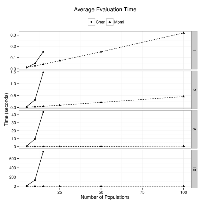
Figure 4: Average computation time per joint SFS entry. For each combination of the number $\mathcal{D}$ of populations and the sample size $n/\mathcal{D}$ per population, we generated 20 random datasets, each under a demographic history that is a random binary tree. The expected joint SFS for the resulting segregating sites were then computed using our method (momi) and that of Chen [8]. Average runtime (in seconds) per joint SFS entry is plotted on the $y$-axis, with each panel corresponding to a different value of $n/\mathcal{D}$. As the plots show, our algorithm is orders of magnitude faster than Chen’s. Due to its significantly increased runtime, we were able to run Chen’s method only up to $\mathcal{D}=15$.

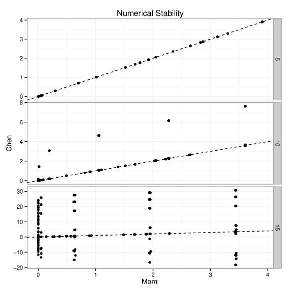
Figure 5: Numerical stability of the two algorithms. The plot compares the numerical values returned by our method (momi) and Chen’s method, for the simulations described in Figure 4. The three panels on the $y$-axis correspond to $\mathcal{D}\in\{5,10,15\}$. To adequately illustrate the observed range of numerical values, the SFS values were transformed via the map $z\mapsto{\rm sign}(z)\log_{10}(1+|z|)$; the dashed line represents the identity $y=x$. The two methods agree for $\mathcal{D}\leq 5$, but Chen’s method displays considerable numerical instability for $\mathcal{D}\geq 10$.

We implemented our formulas and algorithm in Python, using the Python packages numpy and scipy. We also implemented the formulas from Chen [8, 9], and compared the performance of the two algorithms on simulated data.

We simulated data for demographic trees with $\mathcal{D}\in\{5,10,15,25,50,100\}$ populations at the present, and $\frac{n}{\mathcal{D}}\in\{1,2,5,10\}$ individuals per population. For each value of $n,\mathcal{D}$, we used the program scrm [40] to generate 20 random datasets, each with a demographic history that is a random binary tree.

In Figure 4, we compare the running time of the original algorithm of Chen [8, 9] against our new algorithm that utilizes the formulas for $f_{n}^{\tau}(k)$ presented in Section 2 and our new Moran-based approach described in Section 3.2. We find our algorithm to be orders of magnitude faster; the difference is especially pronounced as the number $\mathcal{D}$ of populations grows. Note that, due to the increased running time, we were only able to run Chen’s algorithm to completion for $\mathcal{D}\leq 15$.

In Figure 5, we compare the accuracy of the two algorithms. The figure compares the SFS entries returned by the two methods across a subset of the simulations depicted in Figure 4. To adequately capture the large range of numerical values returned by the Chen method, we transformed each SFS entry using the transformation $z\mapsto{\rm sign}(z)\log_{10}(1+|z|)$. The line $y=x$ is also plotted; points falling on the line depict the SFS entries where both methods agreed. All negative return values represent numerical errors. The two methods agree for $\mathcal{D}\leq 5$, but Chen’s algorithm displays considerable numerical instability for $\mathcal{D}=10$ and higher.

5 Proofs

In this section, we provide proofs of the mathematical results presented in earlier sections.

5.1 A recursion for efficiently computing $\mathbb{P}_{\nu}(A^{\mathcal{C}}_{\tau}=m)$

We describe how to compute $\mathbb{P}_{\nu}(A^{\mathcal{C}}_{\tau}=m)$, for all values of $m\leq\nu\leq n$, in $O(n^{2})$ time. First, note that

$$\mathbb{P}_{\nu-1}(A^{\mathcal{C}}_{\tau}=m)$$

$$= \mathbb{P}_{\nu}(A^{\mathcal{C}}_{\tau}=m+1,\{\nu\}\in\mathcal{C}_{\tau})+\mathbb{P}_{\nu}(A^{\mathcal{C}}_{\tau}=m,\{\nu\}\notin\mathcal{C}_{\tau})$$

$$= \frac{(m+1)p_{\nu,m+1}^{1,1}}{{\nu\choose 1}}\mathbb{P}_{\nu}(A^{\mathcal{C}}_{\tau}=m+1)+\left(1-\frac{mp_{\nu,m}^{1,1}}{{\nu\choose 1}}\right)\mathbb{P}_{\nu}(A^{\mathcal{C}}_{\tau}=m)$$

$$= \frac{(m+1)(m)}{\nu(\nu-1)}\mathbb{P}_{\nu}(A^{\mathcal{C}}_{\tau}=m+1)+\left(1-\frac{m(m-1)}{\nu(\nu-1)}\right)\mathbb{P}_{\nu}(A^{\mathcal{C}}_{\tau}=m).$$

Rearranging, we get the recursion

$$\mathbb{P}_{\nu}(A^{\mathcal{C}}_{\tau}=m)=\frac{1}{1-\frac{m(m-1)}{\nu(\nu-1)}}\left[\mathbb{P}_{\nu-1}(A^{\mathcal{C}}_{\tau}=m)-\frac{(m+1)(m)}{\nu(\nu-1)}\mathbb{P}_{\nu}(A^{\mathcal{C}}_{\tau}=m+1)\right]$$ (20)

with base cases

$$\mathbb{P}_{\nu}(A^{\mathcal{C}}_{\tau}=\nu) = e^{-{\nu\choose 2}\int_{0}^{\tau}\alpha(t)dt}.$$

So after solving $\int_{0}^{\tau}\alpha(t)dt$, we can use the recursion and memoization to solve for all of the $O(n^{2})$ terms $\mathbb{P}_{\nu}(A^{\mathcal{C}}_{\tau}=m)$ in $O(n^{2})$ time. In particular, in the case of constant population size, $\alpha(t)=\alpha$, the base case is given by

$$\mathbb{P}_{\nu}(A^{\mathcal{C}}_{\tau}=\nu) = e^{-{\nu\choose 2}\alpha\tau},$$

and in the case of an exponentially growing population size, $\alpha(t)=\alpha(\tau)e^{\beta(\tau-t)}$, the base case is given by

$$\mathbb{P}_{\nu}(A^{\mathcal{C}}_{\tau}=\nu) = e^{-{\nu\choose 2}\alpha(\tau)(e^{\beta\tau}-\frac{1}{\beta})}.$$

5.2 Proof of Lemma 1

Let $T_{\text{\scriptsize MRCA}}$ denote the time to the most recent common ancestor of the sample. We first note that

$$f_{n}^{\tau}(n) = \tau-\mathbb{E}_{n}[T_{\text{\scriptsize MRCA}}\wedge\tau],$$

since the branch length subtending the whole sample is the time between $\tau$ and $T_{\text{\scriptsize MRCA}}$.

Next, note that $\frac{\theta}{2}\mathbb{E}_{n}[T_{\text{\scriptsize MRCA}}\wedge\tau]$ is equal to the number of polymorphic mutations in $[0,\tau)$ where the individual “1” is derived. This is because, as we trace the ancestry of “1” backwards in time, all mutations hitting the lineage below $T_{\text{\scriptsize MRCA}}$ are polymorphic, while all mutations hitting above $T_{\text{\scriptsize MRCA}}$ are monomorphic.

The expected number of polymorphic mutations with “1” derived is also equal to $\frac{\theta}{2}\sum_{k=1}^{n-1}\frac{k}{n}f_{n}^{\tau}(k)$, since if a mutation has $k$ derived leaves, the chance that “1” is in the derived set is $\frac{k}{n}$. Thus,

$$\mathbb{E}_{n}[T_{\text{\scriptsize MRCA}}\wedge\tau] = \sum_{k=1}^{n-1}\frac{k}{n}f_{n}^{\tau}(k),$$

which completes the proof.

5.3 Proof of Lemma 2

We first note that

$$\mathbb{P}_{n}(\mathcal{M}^{\tau}=\{1,\ldots,k\})$$

$$= \mathbb{P}_{n+1}(\mathcal{M}^{\tau}=\{1,\ldots,k\})+\mathbb{P}_{n+1}(\mathcal{M}^{\tau}=\{1,\ldots,k,n+1\}).$$

By exchangeability, we have $\mathbb{P}_{n}(\mathcal{M}^{\tau}=K)=\frac{\theta}{2}\frac{f_{n}^{\tau}(|K|)}{{n\choose|K|}}+o(\theta)$ for all $K\subseteq\{1,\ldots,n\}$, so

$$\frac{1}{{n\choose k}}f_{n}^{\tau}(k) = \frac{1}{{n+1\choose k}}f_{n+1}^{\tau}(k)+\frac{1}{{n+1\choose k+1}}f_{n+1}^{\tau}(k+1).$$

Multiplying both sides by ${n\choose k}$ gives

$$f_{n}^{\tau}(k) = \frac{n-k+1}{n+1}f_{n+1}^{\tau}(k)+\frac{k+1}{n+1}f_{n+1}^{\tau}(k+1).$$

5.4 Proof of Lemma 3

Let $\alpha^{*}(t)$ denote the inverse population size history given by

$$\alpha^{*}(t) = \begin{cases}\alpha(t)&\text{if }t<\tau\\ \infty&\text{if }t\geq\tau.\end{cases}$$

So the demographic history with population size $\frac{1}{\alpha^{*}(t)}$ agrees with the original history up to time $\tau$, at which point the population size drops to $0$, and all lineages instantly coalesce into a single lineage with probability $1$.

Let $T_{m,*}$ denote the amount of time there are $m$ ancestral lineages for the coalescent with size history $\frac{1}{\alpha^{*}(t)}$. Similarly, let $f_{n,*}(k)$ denote the SFS under the size history $\frac{1}{\alpha^{*}(t)}$. Then from the result of Polanski and Kimmel [37],

$$f_{n,*}(k)=\sum_{m=2}^{n}W_{n,k,m}\mathbb{E}_{m}[T_{m,*}].$$

Note that for $m>1$, we almost surely have $T_{m,*}=T^{\tau}_{m,*}$, i.e. the intercoalescence time equals its truncated version, since all lineages coalesce instantly at $\tau$ with probability $1$. Thus, $\mathbb{E}_{m}[T_{m,*}]=\mathbb{E}_{m}[T^{\tau}_{m,*}]$. Similarly, for $k<n$, $f_{n,*}(k)=f^{\tau}_{n,*}(k)$, i.e. the SFS equals the truncated SFS, because the probability of a polymorphic mutation occurring in $[\tau,\infty)$ is $0$.

Finally, note that $\mathbb{E}_{m}[T^{\tau}_{m,*}]=\mathbb{E}_{m}[T^{\tau}_{m}]$ and $f^{\tau}_{n,*}(k)=f^{\tau}_{n}(k)$, because $\alpha(t)$ and $\alpha^{*}(t)$ are identical on $[0,\tau)$.

5.5 Proof of Proposition 1

We start by showing that $\mathbb{P}_{n}(A^{\mathcal{K}}_{\tau}=m)=\mathbb{P}_{n}(A^{\mathcal{C}}_{\tau}=m)+O(\theta)$. Let $T_{i}^{\tau}(\mathcal{K})=\int_{0}^{\tau}\mathbb{I}_{A^{\mathcal{K}}_{t}=i}dt$ denote the amount of time where $\mathcal{K}$ has $i$ unkilled lineages. Let $p$ denote the probability density function. For $(t_{n},\ldots,t_{m})$ with $\sum t_{i}=\tau$, we have

$$p(T_{n}^{\tau}(\mathcal{K})=t_{n},\ldots,T_{m}^{\tau}(\mathcal{K})=t_{m})$$

$$= e^{-\lambda^{\mathcal{K}}_{m,m-1}t_{m}}\prod_{i=m+1}^{n}\lambda^{\mathcal{K}}_{i,i-1}e^{-\lambda^{\mathcal{K}}_{i,i-1}t_{i}}$$

$$= e^{-\left({m\choose 2}\alpha+\frac{m\theta}{2}\right)t_{m}}\prod_{i=m+1}^{n}\left({i\choose 2}\alpha+\frac{i\theta}{2}\right)e^{-\left({i\choose 2}\alpha+\frac{i\theta}{2}\right)t_{i}}$$

$$= e^{-{m\choose 2}\alpha t_{m}}\prod_{i=m+1}^{n}{i\choose 2}\alpha e^{-{i\choose 2}\alpha t_{i}}+O(\theta)$$

$$= p(T_{n}^{\tau}=t_{n},\ldots,T_{m}^{\tau}=t_{m})+O(\theta),$$

and so

$$\lim_{\theta\to 0}\mathbb{P}_{n}(A^{\mathcal{K}}_{\tau}=m) = \lim_{\theta\to 0}\int_{\sum t_{i}=\tau}p(T_{n}^{\tau}(\mathcal{K})=t_{n},\ldots,T_{m}^{\tau}(\mathcal{K})=t_{m})d\mathbf{t}$$

$$= \int_{\sum t_{i}=\tau}p(T_{n}^{\tau}=t_{n},\ldots,T_{m}^{\tau}=t_{m})d\mathbf{t}$$

$$= \mathbb{P}_{n}(A^{\mathcal{C}}_{\tau}=m).$$

where we can exchange the limit and the integral by the Bounded Convergence Theorem, because $p(T_{n}^{\tau}(\mathcal{K})=t_{n},\ldots,T_{m}^{\tau}(\mathcal{K})=t_{m})\leq\prod_{i=m+1}^{n}\left({i\choose 2}\alpha+\frac{i}{2}\right)$ for $\theta\leq 1$.

Thus we have

$$\mathbb{P}_{n}(|\mathcal{M}^{\tau}|=k,A^{\mathcal{K}}_{\tau}=m) = \mathbb{P}_{n}(|\mathcal{M}^{\tau}|=k\mid A^{\mathcal{K}}_{\tau}=m)\mathbb{P}_{n}(A^{\mathcal{K}}_{\tau}=m)$$

$$= \left(\frac{\theta}{2}f_{n}^{\tau}(k\mid A^{\mathcal{K}}_{\tau}=m)+o(\theta)\right)\left(\mathbb{P}_{n}(A^{\mathcal{C}}_{\tau}=m)+O(\theta)\right)$$

$$= \frac{\theta}{2}f_{n}^{\tau}(k\mid A^{\mathcal{K}}_{\tau}=m)\mathbb{P}_{n}(A^{\mathcal{C}}_{\tau}=m)+o(\theta),$$

which proves the first part of the proposition.

We next solve for $f_{n}^{\tau}(k\mid A^{\mathcal{K}}_{\tau}=m)$, the first order Taylor series coefficient for $\mathbb{P}_{n}(|\mathcal{M}^{\tau}|=k\mid A^{\mathcal{K}}_{\tau}=m)$ in the mutation rate $\frac{\theta}{2}$.

When there are $i$ unkilled lineages, the probability that the next event is a killing event is $\frac{\theta}{\alpha(i-1)+\theta}=\frac{\theta}{\alpha(i-1)}+o(\theta)$. Given that the event is a killing, the chance that the killed lineage has $k$ leaf descendants is $p_{n,i}^{k,1}$. So summing over $i$, and dividing out the mutation rate $\frac{\theta}{2}$, we get

$$f_{n}^{\tau}(k\mid A^{\mathcal{K}}_{\tau}=m) = \frac{2}{\alpha}\sum_{i=m+1}^{n-k+1}\frac{1}{i-1}p_{n,i}^{k,1}$$

$$= \frac{2}{\alpha}\sum_{i=m+1}^{n-k+1}\frac{1}{i-1}\frac{{n-k-1\choose i-2}}{{n-1\choose i-1}}$$

$$= \frac{2}{\alpha}\sum_{i=m+1}^{n-k+1}\frac{1}{i-1}\frac{(n-k-1)!(i-1)!(n-i)!}{(i-2)!(n-k-i+1)!(n-1)!}$$

$$= \frac{2(n-k-1)!}{\alpha(n-1)!}\sum_{i=m+1}^{n-k+1}\frac{(n-i)!}{(n-k-i+1)!}$$

$$= \frac{2(n-k-1)!}{\alpha(n-1)!}\sum_{j=0}^{n-k-m}\frac{(j+k-1)!}{j!}$$

$$= \frac{2}{\alpha k{n-1\choose k}}\sum_{j=0}^{n-k-m}{j+k-1\choose j}$$

$$= \frac{2}{\alpha k}\frac{{n-m\choose k}}{{n-1\choose k}},$$

where we made the change of variables $j=n-k-i+1$, and where the final line follows from repeated application of the combinatorial identity ${a\choose b}={a-1\choose b}+{a-1\choose b-1}$.

5.5.1 Alternative proof for $f_{n}^{\tau}(k\mid A^{\mathcal{K}}_{\tau}=m)$ via the Chinese Restaurant Process

We sketch an alternative proof of the expression for $f_{n}^{\tau}(k\mid A^{\mathcal{K}}_{\tau}=m)$, using the Chinese Restaurant Process.

Consider the coalescent with killing going forward in time (towards the present), and only looking at it when the number of individuals increases. Then when there are $i$ lineages, a new mutation occurs with probability $\frac{\theta}{\alpha i+\theta}=\frac{\theta/\alpha}{i+\theta/\alpha}$, and each lineage branches with probability $\frac{\alpha}{\alpha i+\theta}=\frac{1}{i+\theta/\alpha}$. Thus, conditional on $A^{\mathcal{K}}_{\tau}=m$, the distribution on $\mathcal{K}_{\tau}$ is given by a Chinese Restaurant Process [2], starting with $m$ tables each with $1$ person, and with new tables founded with parameter $\theta/\alpha$.

Let $(x)_{i\uparrow}=x(x+1)\cdots(x+i-1)$ denote the rising factorial. If there is a single mutation with $k$ descendants, then there are ${n-m\choose k}$ ways to pick which of the $n-m$ events involve mutant lineages. The probability of a particular such ordering is

$$\frac{\theta}{\alpha}\frac{(1)_{k\uparrow}(m)_{n-k-m\uparrow}}{(m+\theta/\alpha)_{n-m\uparrow}} = \frac{\theta}{\alpha}\frac{(k-1)!(n-k-1)!/m!}{(n-1)!/m!}+o(\theta).$$

Summing over all ${n-m\choose k}$ orderings, and dividing by $\frac{\theta}{2}$, yields

$$f_{n}^{\tau}(k\mid A^{\mathcal{K}}_{\tau}=m) =\frac{2}{\alpha}{n-m\choose k}\frac{(k-1)!(n-k-1)!/m!}{(n-1)!/m!}.$$

References

- Al-Mohy and Higham [2011] {barticle}[author] \bauthor\bsnmAl-Mohy, \bfnmAwad H.\binitsA. H. and \bauthor\bsnmHigham, \bfnmNicholas J.\binitsN. J. (\byear2011). \btitleComputing the Action of the Matrix Exponential, with an Application to Exponential Integrators. \bjournalSIAM Journal on Scientific Computing \bvolume33 (2) \bpages488–511. \endbibitem
- Aldous [1985] {bincollection}[author] \bauthor\bsnmAldous, \bfnmDavid J\binitsD. J. (\byear1985). \btitleExchangeability and related topics. In \bbooktitleÉcole d’Été de Probabilités de Saint-Flour XIII — 1983, (\beditor\bfnmP. L.\binitsP. L. \bsnmHennequin, ed.). \bseriesLecture Notes in Mathematics \bvolume1117 \bpages1-198. \bpublisherSpringer Berlin Heidelberg. \endbibitem
- Beaumont and Nichols [1996] {barticle}[author] \bauthor\bsnmBeaumont, \bfnmMark A\binitsM. A. and \bauthor\bsnmNichols, \bfnmRichard A\binitsR. A. (\byear1996). \btitleEvaluating loci for use in the genetic analysis of population structure. \bjournalProceedings of the Royal Society of London. Series B: Biological Sciences \bvolume263 \bpages1619–1626. \endbibitem
- Bhaskar, Kamm and Song [2012] {barticle}[author] \bauthor\bsnmBhaskar, \bfnmA.\binitsA., \bauthor\bsnmKamm, \bfnmJ. A.\binitsJ. A. and \bauthor\bsnmSong, \bfnmY. S.\binitsY. S. (\byear2012). \btitleApproximate sampling formulae for general finite-alleles models of mutation. \bjournalAdvances in Applied Probability \bvolume44 \bpages408-428. \bnote(PMC3953561). \endbibitem
- Bhaskar, Wang and Song [2015] {barticle}[author] \bauthor\bsnmBhaskar, \bfnmA.\binitsA., \bauthor\bsnmWang, \bfnmY. X. Rachel\binitsY. X. R. and \bauthor\bsnmSong, \bfnmY. S.\binitsY. S. (\byear2015). \btitleEfficient inference of population size histories and locus-specific mutation rates from large-sample genomic variation data. \bjournalGenome Research \bvolume25 \bpages268-279. \endbibitem
- Boyko et al. [2008] {barticle}[author] \bauthor\bsnmBoyko, \bfnmAdam R\binitsA. R., \bauthor\bsnmWilliamson, \bfnmScott H\binitsS. H., \bauthor\bsnmIndap, \bfnmAmit R\binitsA. R., \bauthor\bsnmDegenhardt, \bfnmJeremiah D\binitsJ. D., \bauthor\bsnmHernandez, \bfnmRyan D\binitsR. D., \bauthor\bsnmLohmueller, \bfnmKirk E\binitsK. E., \bauthor\bsnmAdams, \bfnmMark D\binitsM. D., \bauthor\bsnmSchmidt, \bfnmSteffen\binitsS., \bauthor\bsnmSninsky, \bfnmJohn J\binitsJ. J., \bauthor\bsnmSunyaev, \bfnmShamil R\binitsS. R. \betalet al. (\byear2008). \btitleAssessing the evolutionary impact of amino acid mutations in the human genome. \bjournalPLoS Genetics \bvolume4 \bpagese1000083. \endbibitem
- Bryant et al. [2012] {barticle}[author] \bauthor\bsnmBryant, \bfnmDavid\binitsD., \bauthor\bsnmBouckaert, \bfnmRemco\binitsR., \bauthor\bsnmFelsenstein, \bfnmJoseph\binitsJ., \bauthor\bsnmRosenberg, \bfnmNoah A.\binitsN. A. and \bauthor\bsnmRoyChoudhury, \bfnmArindam\binitsA. (\byear2012). \btitleInferring species trees directly from biallelic genetic markers: bypassing gene trees in a full coalescent analysis. \bjournalMolecular Biology and Evolution \bvolume29 \bpages1917-1932. \bdoi10.1093/molbev/mss086 \endbibitem
- Chen [2012] {barticle}[author] \bauthor\bsnmChen, \bfnmHua\binitsH. (\byear2012). \btitleThe joint allele frequency spectrum of multiple populations: A coalescent theory approach. \bjournalTheoretical Population Biology \bvolume81 \bpages179–195. \endbibitem
- Chen [2013] {barticle}[author] \bauthor\bsnmChen, \bfnmHua\binitsH. (\byear2013). \btitleIntercoalescence Time Distribution of Incomplete Gene Genealogies in Temporally Varying Populations, and Applications in Population Genetic Inference. \bjournalAnnals of Human Genetics \bvolume77 \bpages158–173. \endbibitem
- Cooley and Tukey [1965] {barticle}[author] \bauthor\bsnmCooley, \bfnmJames W.\binitsJ. W. and \bauthor\bsnmTukey, \bfnmJohn W.\binitsJ. W. (\byear1965). \btitleAn Algorithm for the Machine Calculation of Complex Fourier Series. \bjournalMathematics of Computation \bvolume19 \bpages297-301. \endbibitem
- Coventry et al. [2010] {barticle}[author] \bauthor\bsnmCoventry, \bfnmAlex\binitsA., \bauthor\bsnmBull-Otterson, \bfnmLara M\binitsL. M., \bauthor\bsnmLiu, \bfnmXiaoming\binitsX., \bauthor\bsnmClark, \bfnmAndrew G\binitsA. G., \bauthor\bsnmMaxwell, \bfnmTaylor J\binitsT. J., \bauthor\bsnmCrosby, \bfnmJacy\binitsJ., \bauthor\bsnmHixson, \bfnmJames E\binitsJ. E., \bauthor\bsnmRea, \bfnmThomas J\binitsT. J., \bauthor\bsnmMuzny, \bfnmDonna M\binitsD. M., \bauthor\bsnmLewis, \bfnmLora R\binitsL. R. \betalet al. (\byear2010). \btitleDeep resequencing reveals excess rare recent variants consistent with explosive population growth. \bjournalNature Communications \bvolume1 \bpages131. \endbibitem
- Durrett [2008] {bbook}[author] \bauthor\bsnmDurrett, \bfnmR.\binitsR. (\byear2008). \btitleProbability Models for DNA Sequence Evolution, \bedition2nd ed. \bpublisherSpringer, New York. \endbibitem
- Excoffier et al. [2013] {barticle}[author] \bauthor\bsnmExcoffier, \bfnmLaurent\binitsL., \bauthor\bsnmDupanloup, \bfnmIsabelle\binitsI., \bauthor\bsnmHuerta-Sánchez, \bfnmEmilia\binitsE., \bauthor\bsnmSousa, \bfnmVitor C\binitsV. C. and \bauthor\bsnmFoll, \bfnmMatthieu\binitsM. (\byear2013). \btitleRobust Demographic Inference from Genomic and SNP Data. \bjournalPLoS Genetics \bvolume9 \bpagese1003905. \endbibitem
- Felsenstein [1981] {barticle}[author] \bauthor\bsnmFelsenstein, \bfnmJ.\binitsJ. (\byear1981). \btitleEvolutionary trees from DNA sequences: a maximum likelihood approach. \bjournalJournal of Molecular Evolution \bvolume17 \bpages368–376. \endbibitem
- Fu [1995] {barticle}[author] \bauthor\bsnmFu, \bfnmY. X.\binitsY. X. (\byear1995). \btitleStatistical properties of segregating sites. \bjournalTheoretical Population Biology \bvolume48 \bpages172–197. \endbibitem
- Gazave et al. [2014] {barticle}[author] \bauthor\bsnmGazave, \bfnmElodie\binitsE., \bauthor\bsnmMa, \bfnmLi\binitsL., \bauthor\bsnmChang, \bfnmDiana\binitsD., \bauthor\bsnmCoventry, \bfnmAlex\binitsA., \bauthor\bsnmGao, \bfnmFeng\binitsF., \bauthor\bsnmMuzny, \bfnmDonna\binitsD., \bauthor\bsnmBoerwinkle, \bfnmEric\binitsE., \bauthor\bsnmGibbs, \bfnmRichard A\binitsR. A., \bauthor\bsnmSing, \bfnmCharles F\binitsC. F., \bauthor\bsnmClark, \bfnmAndrew G\binitsA. G. \betalet al. (\byear2014). \btitleNeutral genomic regions refine models of recent rapid human population growth. \bjournalProceedings of the National Academy of Sciences \bvolume111 \bpages757–762. \endbibitem
- Gravel et al. [2011] {barticle}[author] \bauthor\bsnmGravel, \bfnmSimon\binitsS., \bauthor\bsnmHenn, \bfnmBrenna M\binitsB. M., \bauthor\bsnmGutenkunst, \bfnmRyan N\binitsR. N., \bauthor\bsnmIndap, \bfnmAmit R\binitsA. R., \bauthor\bsnmMarth, \bfnmGabor T\binitsG. T., \bauthor\bsnmClark, \bfnmAndrew G\binitsA. G., \bauthor\bsnmYu, \bfnmFuli\binitsF., \bauthor\bsnmGibbs, \bfnmRichard A\binitsR. A., \bauthor\bsnmBustamante, \bfnmCarlos D\binitsC. D., \bauthor\bsnmAltshuler, \bfnmDavid L\binitsD. L. \betalet al. (\byear2011). \btitleDemographic history and rare allele sharing among human populations. \bjournalProceedings of the National Academy of Sciences \bvolume108 \bpages11983–11988. \endbibitem
- Griffiths and Tavaré [1998] {barticle}[author] \bauthor\bsnmGriffiths, \bfnmR. C.\binitsR. C. and \bauthor\bsnmTavaré, \bfnmSimon\binitsS. (\byear1998). \btitleThe age of a mutation in a general coalescent tree. \bjournalCommunications in Statistics. Stochastic Models \bvolume14 \bpages273–295. \endbibitem
- Gutenkunst et al. [2009] {barticle}[author] \bauthor\bsnmGutenkunst, \bfnmRyan N.\binitsR. N., \bauthor\bsnmHernandez, \bfnmRyan D.\binitsR. D., \bauthor\bsnmWilliamson, \bfnmScott H.\binitsS. H. and \bauthor\bsnmBustamante, \bfnmCarlos D.\binitsC. D. (\byear2009). \btitleInferring the Joint Demographic History of Multiple Populations from Multidimensional SNP Frequency Data. \bjournalPLoS Genetics \bvolume5 \bpagese1000695. \endbibitem
- Higham [2002] {bbook}[author] \bauthor\bsnmHigham, \bfnmNicholas J.\binitsN. J. (\byear2002). \btitleAccuracy and Stability of Numerical Algorithms, \bedition2nd ed. \bpublisherSIAM: Society for Industrial and Applied Mathematics. \endbibitem
- Hoppe [1984] {barticle}[author] \bauthor\bsnmHoppe, \bfnmF.\binitsF. (\byear1984). \btitlePólya-like urns and the Ewens’ sampling formula. \bjournalJ. Math. Biol. \bvolume20 \bpages91-94. \endbibitem
- Jenkins, Mueller and Song [2014] {barticle}[author] \bauthor\bsnmJenkins, \bfnmPaul A\binitsP. A., \bauthor\bsnmMueller, \bfnmJonas W\binitsJ. W. and \bauthor\bsnmSong, \bfnmYun S\binitsY. S. (\byear2014). \btitleGeneral triallelic frequency spectrum under demographic models with variable population size. \bjournalGenetics \bvolume196 \bpages295–311. \bnote(PMC3872192). \endbibitem
- Jenkins and Song [2011] {barticle}[author] \bauthor\bsnmJenkins, \bfnmP. A.\binitsP. A. and \bauthor\bsnmSong, \bfnmY. S.\binitsY. S. (\byear2011). \btitleThe effect of recurrent mutation on the frequency spectrum of a segregating site and the age of an allele. \bjournalTheoretical Population Biology \bvolume80 \bpages158–173. \bnote(PMC3143209). \endbibitem
- Johnson and Kotz [1977] {bbook}[author] \bauthor\bsnmJohnson, \bfnmNorman Lloyd\binitsN. L. and \bauthor\bsnmKotz, \bfnmSamuel\binitsS. (\byear1977). \btitleUrn Models and Their Application: An Approach to Modern Discrete Probability Theory. \bpublisherWiley New York. \endbibitem
- Kimura [1955] {barticle}[author] \bauthor\bsnmKimura, \bfnmMotoo\binitsM. (\byear1955). \btitleSolution of a process of random genetic drift with a continuous model. \bjournalProceedings of the National Academy of Sciences \bvolume41 \bpages144–150. \endbibitem
- Kimura [1969] {barticle}[author] \bauthor\bsnmKimura, \bfnmMotoo\binitsM. (\byear1969). \btitleThe number of heterozygous nucleotide sites maintained in a finite population due to steady flux of mutations. \bjournalGenetics \bvolume61 \bpages893. \endbibitem
- Kingman [1982a] {barticle}[author] \bauthor\bsnmKingman, \bfnmJ. F. C.\binitsJ. F. C. (\byear1982a). \btitleThe coalescent. \bjournalStoch. Process. Appl. \bvolume13 \bpages235-248. \endbibitem
- Kingman [1982b] {barticle}[author] \bauthor\bsnmKingman, \bfnmJ. F. C.\binitsJ. F. C. (\byear1982b). \btitleOn the genealogy of large populations. \bjournalJ. Appl. Prob. \bvolume19A \bpages27-43. \endbibitem
- Kingman [1982c] {bincollection}[author] \bauthor\bsnmKingman, \bfnmJ. F. C.\binitsJ. F. C. (\byear1982c). \btitleExchangeability and the evolution of large populations. In \bbooktitleExchangeability in Probability and Statistics (\beditor\bfnmG.\binitsG. \bsnmKoch and \beditor\bfnmF.\binitsF. \bsnmSpizzichino, eds.) \bpages97–112. \bpublisherNorth-Holland Publishing Company. \endbibitem
- Lauritzen and Spiegelhalter [1988] {barticle}[author] \bauthor\bsnmLauritzen, \bfnmS. L.\binitsS. L. and \bauthor\bsnmSpiegelhalter, \bfnmD. J.\binitsD. J. (\byear1988). \btitleLocal Computations with Probabilities on Graphical Structures and Their Application to Expert Systems. \bjournalJournal of the Royal Statistical Society. Series B (Methodological) \bvolume50 \bpages157-224. \endbibitem
- Lukić and Hey [2012] {barticle}[author] \bauthor\bsnmLukić, \bfnmSergio\binitsS. and \bauthor\bsnmHey, \bfnmJody\binitsJ. (\byear2012). \btitleDemographic inference using spectral methods on SNP data, with an analysis of the human out-of-Africa expansion. \bjournalGenetics \bvolume192 \bpages619–639. \endbibitem
- Moran [1958] {barticle}[author] \bauthor\bsnmMoran, \bfnmP. A. P.\binitsP. A. P. (\byear1958). \btitleRandom processes in genetics. \bjournalMathematical Proceedings of the Cambridge Philosophical Society \bvolume54 \bpages60–71. \bdoi10.1017/S0305004100033193 \endbibitem
- Nelson et al. [2012] {barticle}[author] \bauthor\bsnmNelson, \bfnmMatthew R\binitsM. R., \bauthor\bsnmWegmann, \bfnmDaniel\binitsD., \bauthor\bsnmEhm, \bfnmMargaret G\binitsM. G., \bauthor\bsnmKessner, \bfnmDarren\binitsD., \bauthor\bsnmJean, \bfnmPamela St\binitsP. S., \bauthor\bsnmVerzilli, \bfnmClaudio\binitsC., \bauthor\bsnmShen, \bfnmJudong\binitsJ., \bauthor\bsnmTang, \bfnmZhengzheng\binitsZ., \bauthor\bsnmBacanu, \bfnmSilviu-Alin\binitsS.-A., \bauthor\bsnmFraser, \bfnmDana\binitsD. \betalet al. (\byear2012). \btitleAn Abundance of Rare Functional Variants in 202 Drug Target Genes Sequenced in 14,002 People. \bjournalScience \bvolume337 \bpages100–104. \endbibitem
- Nielsen [2000] {barticle}[author] \bauthor\bsnmNielsen, \bfnmRasmus\binitsR. (\byear2000). \btitleEstimation of population parameters and recombination rates from single nucleotide polymorphisms. \bjournalGenetics \bvolume154 \bpages931–942. \endbibitem
- Pearl [1982] {binproceedings}[author] \bauthor\bsnmPearl, \bfnmJudea\binitsJ. (\byear1982). \btitleReverend Bayes on inference engines: a distributed hierarchical approach. In \bbooktitleProceedings of the National Conference on Artificial Intelligence \bpages133–136. \endbibitem
- Polanski, Bobrowski and Kimmel [2003] {barticle}[author] \bauthor\bsnmPolanski, \bfnmAndrzej\binitsA., \bauthor\bsnmBobrowski, \bfnmAdam\binitsA. and \bauthor\bsnmKimmel, \bfnmMarek\binitsM. (\byear2003). \btitleA note on distributions of times to coalescence, under time-dependent population size. \bjournalTheoretical Population Biology \bvolume63 \bpages33–40. \endbibitem
- Polanski and Kimmel [2003] {barticle}[author] \bauthor\bsnmPolanski, \bfnmAndrzej\binitsA. and \bauthor\bsnmKimmel, \bfnmMarek\binitsM. (\byear2003). \btitleNew Explicit Expressions for Relative Frequencies of Single-Nucleotide Polymorphisms With Application to Statistical Inference on Population Growth. \bjournalGenetics \bvolume165 \bpages427–436. \endbibitem
- Schaffner et al. [2005] {barticle}[author] \bauthor\bsnmSchaffner, \bfnmS. F.\binitsS. F., \bauthor\bsnmFoo, \bfnmC.\binitsC., \bauthor\bsnmGabriel, \bfnmS.\binitsS., \bauthor\bsnmReich, \bfnmD.\binitsD., \bauthor\bsnmDaly, \bfnmW. J.\binitsW. J. and \bauthor\bsnmAltshuler, \bfnmD.\binitsD. (\byear2005). \btitleCalibrating a coalescent simulation of human genome sequence variation. \bjournalGenome Res. \bvolume15 \bpages1576-1583. \endbibitem
- Sidje [1998] {barticle}[author] \bauthor\bsnmSidje, \bfnmRoger B.\binitsR. B. (\byear1998). \btitleExpokit: A Software Package for Computing Matrix Exponentials. \bjournalACM Trans. Math. Softw. \bvolume24 \bpages130–156. \bdoi10.1145/285861.285868 \endbibitem
- Staab et al. [2015] {barticle}[author] \bauthor\bsnmStaab, \bfnmPaul R\binitsP. R., \bauthor\bsnmZhu, \bfnmSha\binitsS., \bauthor\bsnmMetzler, \bfnmDirk\binitsD. and \bauthor\bsnmLunter, \bfnmGerton\binitsG. (\byear2015). \btitlescrm: efficiently simulating long sequences using the approximated coalescent with recombination. \bjournalBioinformatics \bpagesbtu861. \endbibitem
- Tavaré [1984] {barticle}[author] \bauthor\bsnmTavaré, \bfnmS.\binitsS. (\byear1984). \btitleLine-of-descent and genealogical processes, and their applications in population genetics models. \bjournalTheoretical Population Biology \bvolume26 \bpages119–164. \endbibitem
- Wakeley and Hey [1997] {barticle}[author] \bauthor\bsnmWakeley, \bfnmJohn\binitsJ. and \bauthor\bsnmHey, \bfnmJody\binitsJ. (\byear1997). \btitleEstimating ancestral population parameters. \bjournalGenetics \bvolume145 \bpages847–855. \endbibitem