T3PS v1.0: Tool for Parallel Processing in Parameter Scans

Vinzenz Maurer

Department of Physics, University of Basel,

Klingelbergstr. 82, CH-4056 Basel, Switzerland

T3PS is a program that can be used to quickly design and perform parameter scans while easily taking advantage of the multi-core architecture of current processors. It takes an easy to read and write parameter scan definition file format as input. Based on the parameter ranges and other options contained therein, it distributes the calculation of the parameter space over multiple processes and possibly computers. The derived data is saved in a plain text file format readable by most plotting software. The supported scanning strategies include: grid scan, random scan, Markov Chain Monte Carlo, numerical optimization. Several example parameter scans are shown and compared with results in the literature.

Disclaimer:

T3PS is published under the GNU General Public License . This means that you can use it for free. We have tested this software and its results, but we can’t guarantee that this software works correctly or that the results derived using it are correct.

If you encounter any problem or have a question, feel free to contact the author by e-mail.

1 Introduction

T3PS is a Python program that facilitates swift and versatile implementation of parameter scans on multiple CPUs and/or computers.

Its main focus lies in delegation of tasks (“points” in parameter space) to sub-processes (“point processors”, see 2.2.5) that calculate information about these points. These sub-processes can run in parallel on one or more computers. To this end, each evaluation of a point works the following way:

Each point is characterized by a list of values with fixed length. These values are substituted into a template file in pre-determined positions. The file is then saved into a separate temporary folder and its path is given to a point processor, which returns the results derived from the substituted template file as another list of numbers. These numbers are then saved together with the previous list separated by tabulators (“\t”) to a result file as a single line. Calculations can be interrupted and resumed at any time.

For determining which points should be processed, the following strategies are implemented in T3PS:

• Simple scan: the user directly specifies a grid, basic probability distributions or an explicit list of points that shall all be processed.

• Markov Chain Monte Carlo (MCMC) algorithm: the user specifies ranges or discrete sets of parameter values, a propagation likelihood and the number of points to calculate to obtain a sample for the likelihood in question.

• Optimizing scan: the user specifies ranges or discrete sets for the values of the defined parameters. Using an evolutionary algorithm, the global maximum of a user-supplied fitness function is searched for.

• Exploring scan: the user specifies a grid of points and a likelihood function. The points will be calculated gradually while aiming to find more likely or more interesting points earlier than others.

Additionally, T3PS supports the following auxiliary modes:

• Test mode: point values are provided by hand by the user. This is useful for checking the implementation of a given point processor and scan definition before committing to a lengthy parameter scan.

• Worker mode: This mode is used only in setups involving multiple computers. In this mode, the running instance of T3PS does not come up with new points on its own but rather waits for a “manager” process to supply them.

This manual is organized the following way: after a quick introduction to T3PS in sec. 1.2, the general structure, strategies and concepts of typical parameter scans are shown in 2. In sec. 3, the scan definition format is introduced and all possible definition directives are listed and explained. The command line interface is detailed in sec. 4. In sec. 5, the implementation of multi-computer calculations is described. Finally in sec. 6, the already implemented and included point processors are documented. Everything is put together in several example scans in sec. 7.

1.1 System Requirements

The following software packages must be installed for T3PS to run:

• Python 2.7 or compatible, e.g. PyPy 1.5 or higher

• Unix-like operating system

1.2 Installation and Quick Start

T3PS is usable right after extracting its archive file and possibly making the main file executable:

⬇

$ tar xvfz T3PS-1.0.tar.gz

$ cd T3PS-1.0

$ chmod u+x src/t3ps

$ ./src/t3psscan_definition.scan

For easier usage, it can also be properly installed using

⬇

$ make install

which (after a prompt to the user) will copy T3PS to an installation folder and will create a link such that T3PS can be launched by simply typing

⬇

$ t3ps

As an introduction, we will now show how to perform a very basic scan. We begin with the scan definition file called “QuickStart.scan”:

⬇

[setup]

point_processor = processors/SimpleProcessor.py

template = QuickStart.function

[SimpleProcessor]

# do a scan with the ‘basic calculator’

# with basic mathematical functions

program = bc --mathlib

[parameter_space]

# two parameters called x and y

par_names = x, y

# define each parameter to take 100 different

# values going from -1 to 1

par_x = interval(-1, 1) with count = 100

par_y = interval(-1, 1) with count = 100

The point processor called SimpleProcessor (included in the T3PS package) will use the basic calculator bc to calculate the mathematical function $\sin(x^{2}+y)\cos(y^{2}+3x)$ by inserting the $x$ and $y$ values into the template file with the name “QuickStart.function” and the following content:

⬇

s( ($x)^2 + ($y) ) * c( ($y)^2 + 3 * ($x) )

The only thing left to do for the scan is launching T3PS using

⬇

$ t3psQuickStart.scan

After a short while in the command line interface of T3PS, the resulting data set can be plotted in Wolfram Mathematica^®[1] using the code

⬇

points = Import["QuickStart.scan.data", "Table"];

ListContourPlot[points[[All, {1,2,3}]]]

and in gnuplot [2] using the code

⬇

splot "QuickStart.scan.data" using 1:2:3

For examples that go more in-depth and show more features, see sec. 7.

2 Overview

Figure 1: Flow chart representing the overall algorithmic structure of a scan in T3PS. The main program takes the information provided by the scan definition file and distributes the work to a certain number of concurrently running point processors, one point each. These in turn calculate data using some (possibly external) code and return the relevant data.

2.1 Scanning Strategies

We will now go into more detail how each scanning strategy behaves and is (roughly) implemented. For more detailed sketches of the actual implementations, see app. A.

Scan

This mode simply processes a defined set of points in the specified parameter space. There are three basic modes for specifying it.

In the first mode, the user specifies the parameter space as a grid defined as the direct product of finite ranges for each parameter. It is then scanned over by simple iteration over all points on the grid. This mode is called “grid” mode.

If one or more parameter range is continuous, but the full space is still a direct product, the second mode applies. Here a user-specified number of points in parameter space is randomly chosen (according to their distribution) and calculated. T3PS calls this mode “scatter”.

In the third mode, instead of a parameter space as direct product of ranges, the user can supply a file in tabulator separated values (TSV) format that specifies the set of possible parameter value combinations that constitutes the parameter space. This mode is called “file” mode.

MCMC

This mode uses a standard Metropolis-Hastings algorithm [3, 4] to draw random samples of points from a more complicated probability distribution. This is also known as a Markov Chain Monte Carlo (MCMC) method.

The range for each parameter can either be given a set of discrete and equally probable values or as continuous values following some (simple) probability distribution. In both cases, the user can supply a step size for a Gaussian proposal density around the parameter value of the previous iteration. If no step size is given, the specific point coordinate is chosen at random from their prior probability distribution given by the parameter range definition.

Once a Markov chain reaches a user-supplied number of sample points (not taking into account non-trivial stay counts), it terminates.

For a sketch in pseudocode of the implementation in T3PS, see sec. A.1.

Optimize

This mode implements a differential evolution algorithm [5] to optimize a user-supplied fitness function. Here, T3PS tries to find the global fitness maximum by (starting from a randomly found or user-supplied initial population of points) repeatedly applying an evolutionary approach that yields a new – better or same quality – population in each iteration.

It stops once the best found fitness has not changed by more than a user-supplied threshold value for a user-supplied number of iterations. If the full parameter space has only a finite amount of points, this mode caches calculation results and thus never calculates points twice.

For a sketch in pseudocode of the implementation in T3PS, see sec. A.2.

Explorer

This mode implements a custom swarm type algorithm acting on a discrete finite grid, analogous to the plain “scan” mode. Starting from randomly found or user-supplied points and emanating from further calculated points, the neighbor points (relative to the grid) of a subset of points are calculated in each iteration, where points with a higher value of a user supplied “likelihood” function take precedence over ones with lower values. T3PS keeps track of all calculated points and no point is processed twice (some memory usage optimizations can change this slightly). Since on a finite grid calculation time is also finite, this is just a re-ordering compared to doing the same calculation in “scan” mode. However, if one is only interested in points satisfying a particular needed level of likelihood, this method can save time when dealing with extensive parameter spaces (depending on the starting points), while still benefiting from the regularity and controllable density of grid-form parameter spaces.

An additional feature is the specification of projections over which a function shall be maximized (not necessarily the “likelihood” function). When the user specifies such a projection, T3PS groups up all known points by two (user supplied) coordinates $x$, $y$ and third coordinate $z$ (default is the “likelihood”). Then the points with maximal $z$ coordinate $z_{\max}$ for each point in the $x$, $y$ plain are used first as site for the calculation of further neighbor points. In addition to simple neighbors, these optimal points are interpolated and extrapolated to smoothen out the projected $x$-$y$-$z_{\max}$ graph.

More specifically, the algorithm has three states. In state one, only one point with maximal $z$ per $x$ and $y$ is found and has his neighbor points and extra-/interpolated pseudo-neighbors calculated. If the algorithm does not find any new points this way, it goes into state two and instead looks for the points maximizing $z$ while being on the boundary of the point set, i.e. ones that have some missing neighbors, and calculates those missing neighbors. In the case, where the algorithm does not find any new points in state two, it goes into state three, where projections are not considered and just a set of pre-defined number of boundary points with sufficient likelihood has their neighbors calculated.

If there are no projections defined, the algorithm always automatically goes into state three. If there are projections defined, every time new points are found the algorithm reverts back to state one.

Moreover, in the case where approximate symmetries of the parameters are known under which the results are almost invariant, these can also be specified and used in state one to further refine the $x$-$y$-$z_{\max}$ graphs by applying the corresponding transformations to the points with maximal $z$ coordinate in each plain.

Note that there is no automatic convergence analysis and users must decide for themselves whether or not the calculation has run long enough. T3PS only calculates some possibly helpful indicators involving the change in the projection plains and other characteristics between each iteration.

For a sketch in pseudocode of the implementation in T3PS, see sec. A.3.

Worker

As a worker instance, T3PS will not start any calculations on its own, but will listen on a user-supplied network port (default: 31415) for calculation requests from T3PS manager instances. To make sure only appropriate processes make these requests a shared secret also referred to as “authorization key” must be specified. This key has to be distributed among the involved T3PS instances and scan definition files.

For more details on this mode, see sec. 5.

Test

This mode can be used to test the formulas and other general directives given in the scan definition file. For this, T3PS will process points in parameter space that are supplied directly by the user and only indirectly consider parameter ranges specified in the scan definition file. Specifying points can either be done via the command line argument “--pars” (see sec. 4) or directly via a prompt on the terminal. Input via the terminal will be saved for later re-use and can be accessed via arrow up and down keys. Calculation results will also be saved. Additionally, the user can choose to run the calculation on one of the configured T3PS worker instances.

2.2 General Concepts

2.2.1 Running of External Code

To make it possible to run more than one process in parallel, T3PS will create temporary directories, in which each process will run. This means that, in general, external code must make no assumptions on the location of the current directory and must be able to run from any directory on the computer. In addition, any side-effects outside of the current directory should be minimal – this also means that external code should generally be what is usually referred to as “re-entrant”.

2.2.2 Structure and Storage of Results

Every result of processing a parameter point consists of three parts:

Parameters

A parameter is a value taken from a specified range. The parameters directly and uniquely label every point in the parameter space.

Variables

A variable is a simple function of the parameters. They are calculated before substituting anything into the template file. This can be used to re-parametrize the calculation, e.g. from $a,b$ to $a/b,a\cdot b$, or to obtain values following more complicated distributions than what is currently supported for parameters in T3PS.

Data

This denotes all values as derived and returned by the point processor, see sec. 2.2.5.

Each line in the result file is then a tabulator separated list of values consisting of either the concatenation of these three sub-lists of values (customizable in “scan” mode) for valid points or only parameter values and exclusion reason for invalid ones. Each point has to fulfill the following two criteria to be considered valid:

No Error

The point processor must have successfully returned, i.e. no error must have occurred (“Python has not raised an exception”). This usually also means that external programs must have exited with an error code of 0.

Inside Bounds

The three sets of values of above have to satisfy a list of user-supplied bounds/constraints.

The tabulator separated format can be read directly by gnuplot [2] and by Wolfram Mathematica^®[1] (using its Import function).

As result from performing a scan defined in the file “$name$.scan”, T3PS generates the following files in the current working directory:

$name$.scan.log

Log file containing the most important messages from T3PS. (Mode: all)

$name$.scan.data

Valid result points. One line per point in parameter space, tabulator separated values. In “optimize” and “explorer” mode, one additional column is appended containing the fitness function or likelihood value. (Modes: all except test, worker and mcmc)

$name$.scan.excluded-data

Excluded result points. Same format as “.data” files except for a single column prepended containing only the character ‘E’ for error/exclusion. The columns following that contain the parameter values and the reason for exclusion or error message as text. Note that upon importing data formatted like this, T3PS will silently ignore the first column (‘E’). (Modes: all except test, worker and mcmc)

$name$.scan.resume

Current resume position. (Mode: scan)

$name$.scan.speed

Current statistical information on the speed of the calculation. This will be regenerated over time if deleted. (Mode: scan, mcmc)

$name$.scan.testhistory

History of user supplied input points in “test” mode. History file format of readline library. (Mode: test)

$name$.scan.testdata

Valid points obtained during calculations in “test” mode. Same format as “.data” file. Likelihood value is appended to each row if defined. (Mode: test)

$name$.scan.chain.$i$

Valid points obtained from the $i$’th Markov chain (starting from $i=0$). Lines include likelihood and stay count at the end for every point in addition to parameters, variables and data. Otherwise, same format as “.data” file. (Mode: mcmc)

$name$.scan.rejected.$i$

All valid but rejected data points that the $i$’th Markov chain (starting from $i=0$) encountered, i.e. those that were discarded only due to random chance. Rows include the likelihood at the end for every point in addition to parameters, variables and data. Otherwise, same format as “.data” file. (Mode: mcmc)

$name$.scan.work

Set of points that were determined to be calculated next in a previous run of T3PS. This is used to resume calculations without the need to regenerate this information. (Mode: explorer)

$name$.scan.boundary

Cache for the determination of boundary points, i.e. points that are not invalid and have missing neighbor points. (Mode: explorer)

$name$.scan.projectedpoints

Parameter values (TSV format) of the set of points that were determined to have maximal $z$ value in each of the projections. This can be used to do the minimal amount of calculation necessary to re-calculate all projection graphs. This is only updated during state one iterations. (Mode: explorer)

$name$.scan.projection.$i$

The $x$-$y$-$z_{\max}$ graph of the $i$’th projection (starting from $i=0$) in TSV format (only updated in state one). This is also used to assess the difference of the projection plains between successive state one iterations. (Mode: explorer)

$name$.scan.population

Last used population in the differential evolution algorithm. The points are contained as lines consisting of likelihood and parameter values (in that order) separated by tabulator characters. (Mode: optimize)

$name$.scan.optimum

Parameter point that maximizes the likelihood function. Same format as “.population” files. (Mode: optimize)

2.2.3 Formula Input

T3PS understands and uses formulas in the form of Python code in several places in the scan definition file. They are compiled to Python bytecode and evaluated according to the following rules:

• Parameter, variable and data values of each point in parameter space can be accessed using “pars.NAME”, “vars.NAME” and “data.NAME”, where NAME is a name as given in the scan definition file. Alternatively, the syntax “list[$i$]”, where list can be pars, vars or data, can be used to access the value of the $i$’th value with $i$ starting from 0. Note that it is not possible to have unnamed parameters or variables, while unnamed data values are allowed but only at the end of the list of data values and are only accessible using “data[$i$]”.

  In some cases, only a subset of these values can be available, for more details see the relevant formula directive description. For rules on what constitutes a valid name, see the description of par_names in sec. 3.3.

• In Python formula expressions, you can use all built-in Python functions as well as several functions and constants from the Python module “math” simply by name.

  One can provide access to more Python modules using the directive helper_modules in the setup section, see sec. 3.2.

• The output of formulas is assumed to be a single value unless stated otherwise (being something else leads to undefined behavior). If this is not the case, it will be clearly mentioned in the relevant scan definition directive description.

• Formulas for variables are evaluated in the order in which they are saved to the result file. Variables calculated first can not directly depend on variables coming later. However, to circumvent this limitation, T3PS provides the “remember” function to remember values computed in formulas before.

  Usage:

  ⬇

  # setting values

  remember(var=value)

  # retrieving values

  remember("var")

• All formulas are evaluated with Python’s flag for “future division” enabled. This means that contrary to ordinary Python code the division of two integers using the operator ‘/’ yields a floating point number and not an integer. Standard integer division can still be done using ‘//’.

  Example: “1 / 2” $\to 0.5$, “1 // 2” $\to 0$.

• Exceptions/errors (e.g. division by zero or invalid indexing) occurring in formulas for variables and bounds simply count as a reason for exclusion of the parameter point. Exceptions in all other formulas lead to a complete stop of the running scan, unless stated otherwise. It is advised to make use of the “test” mode to catch ill-defined formulas early before they generate large erroneously excluded data sets.

Examples for formulas:

⬇

# A_0 =

pars.a0 * pars.m0

# likelihood for Higgs mass fit =

exp(-0.5 * ((data.mh0 - 125.7) / 0.4) ** 2)

# P_ee (electron neutrino survival probability)

1 - sin(2*pars.theta) ** 2 * sin(

vars.deltam12sqr * pars.L / 4 / pars.E

) ** 2

# bound check for BR(mu -> e gamma)

data.BR_muegamma < 2.4e-12

2.2.4 Template File

The template file is a file containing special text fragments that are replaced with (parameter or variable) values specific to the currently processed point in parameter space. The possible forms for these placeholder text fragments are similar to Unix shell variable interpolation and are given by:

$valueidentifier

This will be replaced with the value corresponding to the point in question. valueidentifier can only contain letters, numbers, underscore and dot. The first character not conforming to this terminates the placeholder specification.

This provides access to parameters and variables of a point through the placeholder fragments “$pars.NAME” and “$vars.NAME” with the same rules for NAME as in input formulas. In addition, both sets of values together can be accessed directly using “$NAME”, where parameter names take precedence before variable names.

${valueidentifier}

Equivalent to the placeholder fragment “$valueidentifier” except that the identifier can also contain the square bracket characters ‘[’ and ‘]’. This is also useful if valid valueidentifier characters follow the placeholder fragment.

Examples:
“${intpart}.${fracpart}”, “${vars[0]}”

$$

This placeholder will be replaced with the letter ‘$’.

In the following, substituted template file will refer to the template file with all of its placeholders replaced with the values belonging to the current point in parameter space.

2.2.5 Point Processor

The point processor is a Python module containing a function “main” with either one or three arguments, namely the path of a substituted template file and parameter and variable values. This function can thus either have the signature

⬇

def main(template_file_path):

or (useful for processors that handle parameters and variables directly; see e.g. sec. 7.2)

⬇

def main(template_file_path, parameter_values, variable_values):

The “main” function must return an object of type “list” (or another iterable type) consisting of the derived values.

For more advanced purposes, the point processor module can additionally contain a function “init”, which is called with the following arguments: the folder of the scan definition file, the Python SafeConfigParser object containing the scan definition directives and the Python module containing all functions and classes of T3PS. It has the signature

⬇

def init(definition_file_path, config_object, module):

This can be used to initialize any internal structures depending on specifics of the scan definition. For an example, see the source code of the “ExampleProcessor” point processor provided with the T3PS package.

In practice, the point processor module’s main function should be as simple as possible and should directly call another process and then parse its output for the data relevant for the calculation. Since each new process that is started during point processing, e.g. a shell or other language interpreter, increases the calculation time, this can lead to – depending on the overall performance – significant delays for large parameter spaces. It is thus recommended to try to minimize the amount of added complexity in the processing of a point.

For an overview of point processors already included in T3PS, see sec. 6.

3 How to define a Scan

This section covers the scan definition file format of T3PS with all currently available directives.

3.1 Definition File Format

The scan definition file format is based on the one accepted and processed by the Python module SafeConfigParser [6], which is very similar to one of standard “.ini” files as used by Microsoft Windows^®. Each file consists of one or more sections labeled by the line “[section_name]”. Each section consists of lines of name, value pairs of the form “name=value” or “name:value”, with names specific to that section. It is not necessary to put quotation marks around a string value. Trailing whitespace in names and leading and trailing whitespace in values as well as trailing whitespace on every line is removed, and multi-line values can be given by indenting lines after the one with “name”. Additionally, all names are case-sensitive and later specifications with the same name and section simply overwrite earlier ones.

Comments are given by lines starting with “#” or “;”. Additionally, comments in otherwise non-empty lines can only be made using “;”, and only if there is whitespace in front of it.

The SafeConfigParser module also supports text substitution. This means values can contain references to other values in the same section (or optionally in a special section called “DEFAULT”). These references are then replaced with the referred to (final) value for the full evaluation of the directives. An example for the scan definition file syntax is given by:

⬇

# comments look like this

[section]

version : 1

information = This config file has one quite long

but uninformative multi-line value

dir = IGNORED

template = %(dir)s/file

point_processor = %(dir)s/FullCalculation.py

dir = folder

one_hundred_percent = 100%%

This replaces the text fragment “%(dir)s” with “folder” in the directives template and point_processor, such that the template directive now has the value “folder/file”. Note that the value “IGNORED” is ignored since it has been overwritten by setting dir a second time. Note that, to write actual ‘%’ characters, one must instead write ‘%%’.

Please keep in mind that text substitution into formulas leads to direct evaluation of the substituted text fragment by Python. Thus the value string “%(x)s ** 2” with x being set to “-1” is substituted by SafeConfigParser to “-1 ** 2”. Due to operator precedence, Python evaluates this expression to $-1$. In contrast, the formula “pars.x ** 2” is correctly evaluated to $+1$.

Beyond the default SafeConfigParser features, T3PS also supports the inclusion of other files using the syntax:

⬇

@include PathToFile

This causes the file accessible under the path “PathToFile” to be parsed directly as is at the position of this statement. In particular, multi-line values can be started in the parent file and be continued in the included file. If the given path is not absolute, the file is looked for in the following folders (in order):

• the current folder, from which T3PS was run.

• the folder containing the main scan definition file, i.e. the one that was not subject to @include somewhere and was given last on the command line if applicable.

• the folder containing the T3PS executable file.

• the folder containing the real T3PS file if it was launched through a symbolic link.

Note that, as usual in Unix shells, paths starting with “~” or “~username” have this initial part replaced with the respective user’s home directory.

3.2 The “setup” Section

This section contains the directives concerning the general setup of the calculation.

version

(integer) This specifies which T3PS version the scan definition is written for. Defaults to $1$.

In future versions of T3PS, this will be used to enable backwards-incompatible features (the default value will not change).

mode

(string) Can be one of “scan”, “mcmc“, “optimize”, “explorer”, “test” or “worker”. Specifies which scanning strategy should be employed. Can be overwritten using the “--mode” command line argument, see sec. 4.

concurrent_processors

(integer) Specifies the number of concurrently running processes that T3PS should use on the running computer. This does not affect worker instances running on other computers. For more details, see sec. 5.

This defaults to the number of processor cores of the running computer.

template

(path) The path to the template file. If this directive is not present, T3PS will not perform the actions outlined in sec. 2.2.4 and the template argument passed to the point processor’s main function will be ‘None’.

This directive follows the same search rules for paths as the “@include” statement.

point_processor

(path) The path to the source code file of the point processor that is used to calculate points. Note that it must be implemented in Python (or as a wrapper written in Python) and must be importable without errors. If not given, T3PS will only calculate variables and no data values.

This directive follows the same search rules for paths as the “@include” statement.

helper_modules

(string) List (separated by ‘:’) of module names or paths to Python module files that shall be made available to the evaluation of input formulas. If given as path to a file, a module can be accessed by its´bare file name, i.e. without folder and extension.

Each module path is resolved using the same search rules for paths as the “@include” statement.

3.3 The “parameter_space” Section

This section can contain the following directives:

par_names

(string) List of names (separated by comma) given to the parameters. Whitespace around list elements is stripped. Names can contain letters, numbers and underscore, but must not start with a number or underscore, must not be empty or a Python keyword and must not be in the list multiple times.

par_$name$

(range) The value range for the parameter called $name$. A valid range is given by “definition [with options], where options can be a comma separated list of “name=value” pairs while definition can be one of the following

• a finite list of numeric values, e.g. “1, 2, 3, 4”. Intermediate values can be replaced with an ellipsis “…” or “..”, with at least two values preceding and one following the ellipsis, e.g. “1, 1.2, ..., 2”. Such an expression “a, b, ..., c” will be expanded to the list of numbers starting at $a$ and going to $c$ with step size $b-a$. Example:

  $$\text{``{\small 1, 1.2, ..., 2}''}\to\{1,1.2,1.4,1.6,1.8,2\}$$

  The values $a$, $b$ and $c$ will always be part of the value range even if $c$ is not exactly encountered using this expansion.

• an interval definition as in “interval(a, b)”. This range type supports the options count and distribution. The latter can be either “linear” or “log” specifying whether the parameter or its logarithm shall be uniformly distributed. If “count” is given, the range is automatically translated into a finite range with appropriate equidistant (linear or log) spacing and as many points. Example:

  “interval(1, 2) with count=5”

  $$\to \{1,1.25,1.5,1.75,2\}$$

• the definition of range with a Gaussian distribution with mean mu and standard deviation sigma written as “normalvariate(mu, sigma)”. This range type also supports the option “count”, which automatically translates the range into a discrete and smoothly spaced set of values also following a normal distribution. Example:

  “normalvariate(1, 2) with count=11”

  $$\to \{-1.77,-0.94,-0.35,0.14,0.58,1.00,1.42,$$

  $$\quad 1.86,2.35,2.94\}$$

In “mcmc”, all parameter ranges can also have the option “mcmc_stepsize”. For details, see sec. 3.5.

var_names

(string) Comma-separated list of names for the variables. Same rules and behavior as for “par_names”.

var_$name$

(formula) Formula for calculation of the variable called $name$. Follows the formula input format detailed in sec. 2.2.3. Can only depend on parameters and constants. Variable formulas are evaluated in the order in which they appear in var_names. Errors (e.g. division by zero or invalid indexing) occurring during the evaluation of these formulas will lead to exclusion of the point.

Examples for variables:

⬇

# Bino mass M_1 = r_1 M_{1/2}

var_M1 = pars.r1 * pars.M12

# Trilinear coupling (A_u)_{33} = A_t y_t

var_Au33 = pars.A_t * (pars.m_t / 174)

data_names

(string) Comma-separated list of names for the data values. Same rules as par_names and var_names. If the point processor returns more values than names are given here, the excess values can be accessed by their index $i$ (starting from 0) using the syntax “data[$i$]”.

bound_count

(integer) The number of user-defined bounds or validity checks performed for each point in parameter space. Defaults to $0$.

bound_$i$

(formula) Formula for the $i$’th constraint check (starting from $i=0$) performed for each (otherwise valid) point in parameter space. Should compute a value that can be interpreted as True or False. Note that you must define at least as many bounds as specified in bound_count, while surplus bounds are ignored.

The check is performed only after the point in parameter space has been handed over to the point processor and the calculation has finished, i.e. “data” values are always available. The constraint checks are not evaluated if the point processor itself has generated an error.

This has the same semantics regarding exceptions/errors as var_$name$, i.e. errors lead to exclusion of the point.

3.4 Scan Mode Specific Directives

In addition to the generally applicable directives above, the “scan” mode has the following modified semantics and directives. Directives written as “[section] name” refer to “name” in the section “section”.

[setup] unit_length

(integer) The number of points that are processed in one batch. This means that for each scan iteration a set of points with length given by this directive of not yet calculated points is selected and handed over to all running point processor processes. The Python multiprocessing module ensures that the set is evenly distributed across all of them. After all points in the set have been processed, the results are saved to the “.data” or “.excluded-data” files (depending on the validity of the specific point).

It is generally advised to set this value high enough so that the waiting time for all processes to finish is not large compared to the full processing time of the set of points in parameter space.

Defaults to $100\,\cdot\,$concurrent_processors.

[parameter_space] mode

(string) Can be either “grid” (default), “scatter” or “file”.

In “grid” mode, the usual interpretation of parameter definitions as described in sec. 3.3 applies and all parameter ranges must be finite.

In “scatter” mode, a random sample of points is drawn from the parameter ranges to be processed. The number of points can be adjusted using the directive point_count in the parameter_space section.

In “file” mode, the parameter space is not given by the Cartesian product of parameter ranges, but by pre-determined parameter space points given in the files in the directive files of the parameter_space section. In this case, the directives “par_$name$” in the parameter_space section are interpreted as input formulas (as detailed in sec. 2.2.3) that, however, only have access to the “file” values instead of “pars”, “vars” or “data”. These “file” values correspond to the columns (tabulator separated) of each line in the files specified in the files directive. They can be accessed by index or via the names specified in the file_columns directive.

[parameter_space] point_count

(integer) The number of points that should be calculated. Only applies in parameter space mode “scatter”.

[parameter_space] files

(string) List of file names separated by ‘:’ (whitespace is significant except for leading and trailing one of full lines!) to be used as definition of the parameter space. Only applicable in “file” parameter space mode (or “explorer” mode).

If the command line parameter --output_dir is set and a path is just a file name, it is first looked for therein. Otherwise, each path is resolved using the same search rules as the “@include” statement. Lines starting with a column containing only ‘E’, i.e. lines containing excluded points, are ignored.

[parameter_space] file_columns

(string) List of names (separated by comma) given to the columns in the files given in the directive files. Same rules and behavior as “par_names”, “var_names” and “data_names”. Only applicable in “file” parameter space mode.

[algorithm] out_columns

(formula) List of formulas separated by commas specifying what values should be saved to the “.data” file. Can be used for e.g. re-ordering or re-parametrizing of the result values. The formulas have access to “pars”, “vars” and “data” (as well as “file” values in “file” mode).

If not given, T3PS saves all data as usual (excluding “file” values).

3.5 MCMC Mode Specific Directives

In addition to the general directives, this mode also has the following changed semantics in the sections setup and parameter_space and its own directives in the algorithm section. Directives written as “[section] name” refer to “name” in the section “section”.

[setup] unit_length

(integer) The number of distinct points, i.e. not weighted by stay count, each Markov chain shall find.

[setup] concurrent_processors

(integer) T3PS runs this many chains in parallel on the local computer.

[parameter_space] par_$name$

(range) In “mcmc” mode, all ranges can also have the option “mcmc_stepsize” that specifies the step size for the Gaussian proposal density around the parameter value of the last iteration. For discrete parameter ranges, this is understood to work on the indices into the list of values, i.e. the result of the proposal density sampling is rounded to the nearest integer).

[algorithm] likelihood

(formula) Formula for the calculation of the propagation likelihood. This formula has to evaluate to non-negative numbers for all valid points in parameter space. Its value is also saved together with the stay count in the resulting “.chain.$i$” files. Points with vanishing likelihood value are always rejected. To fit a data value to a measurement with mean $\mu$ and uncertainty $\sigma$, the likelihood should be given by:

⬇

likelihood = exp(

-(data.x - $\mu$) ** 2 / (2 * $\sigma$ ** 2)

)

Beyond fixing the length of all chains, T3PS does not perform any convergence analysis.

Note that this mode does not support distributing the calculation to more than one computer using the manager/worker architecture. However, since Markov chains work autonomously, this can be done by hand by starting T3PS on each computer in “mcmc” mode separately.

3.6 Optimize Mode Specific Directives

This mode also has slightly adjusted semantics for the scan definition directives. Additionally, there are new directives in the algorithm section, which make it possible to adjust the different parameters of the differential evolution algorithm [5]. Directives written as “[section] name” refer to “name” in the section “section”.

[setup] unit_length

(integer) The used population size. Defaults to $10\,\cdot\,D$, where $D$ is the number of parameters with at least two possible values.

[algorithm] likelihood

(formula) The fitness function that is maximized. No restrictions are placed on its value beyond being a real number.

[algorithm] waiting_threshold

(float) The maximal absolute change in the fitness function that is not considered convergent behavior. Defaults to $0$.

[algorithm] waiting_threshold_relative

(float) The maximal relative change in the fitness function that is not considered convergent behavior. Defaults to $10^{-\eta/2}$, where $\eta$ is given by the machine precision (16 in the case of double precision).

[algorithm] waiting_time

(integer) The number of iterations, during which the change in the likelihood function value is below the one governed by the waiting thresholds, that the algorithm should wait to make sure convergence has really taken place. Defaults to $10\,\cdot\,D$, where $D$ is the number of parameters with at least two possible values.

[algorithm] differential_weight

(float) The differential weight as used in differential evolution, see sec. A.2. Defaults to $0.6$.

[algorithm] crossover_probability

(float) The cross-over probability as is used in differential evolution, see sec. A.2. Defaults to $0.5$.

In summary, the fitness $f$ is considered to have converged if

$$|f_{i}-f_{i+1}|<\epsilon+\rho|f_{i}|\;,$$

for at least waiting_time$+1$ consecutive iterations $i$, where $\epsilon$ is determined by the directive waiting_threshold and $\rho$ by the directive waiting_threshold_relative. Note that, due to the random nature of the algorithm, this does not make a statement on the precision of the obtained optimal point or fitness.

3.7 Explorer Mode Specific Directives

The “explorer” mode has the following semantics and custom directives. Directives written as “[section] name” refer to “name” in the section “section”.

[setup] unit_length

(integer) Generate this many random points as initial point set. During running, neighbors of (at most) this many points are calculated when no projections are done in that iteration, i.e. state three. This directive has no consequence in projection-enabled iterations (state one or two).

Defaults to $10\,\cdot\,D$, where $D$ is the number of parameters with at least two possible values.

[algorithm] loading_filter

(formula) Formula analogous to “bound_$i$” in the section “parameter_space” that can be used to specify a condition that points have to satisfy to be loaded from disk into memory. Note that this only applies to loading, and points calculated afterwards are not filtered by this. If not given, T3PS loads all points.

Note that this may cause T3PS to calculate points twice.

[parameter_space] files

(string) List of file names separated by ‘:’ (whitespace is significant!) to be used as additional source for known parameter space points. T3PS will not write to these files.

If the command line parameter --output_dir is set and a path given here is just a file name, it is first looked for therein. Otherwise, each path is resolved using the same search rules as the “@include” statement.

[algorithm] likelihood

(formula) Formula for the calculation of the likelihood quality criterion for all points. This can be negative.

[algorithm] min_likelihood

(float) The minimal likelihood value that a point in parameter space has to have to be considered for further calculations. Points with values lower than this will still be saved in the “.data” file, but will be treated as invalid for exploration.

[algorithm] likelihood_steps

(string) List of numerical values separated by comma specifying bins into which the likelihood of all points should be categorized. Example for bin interval determinations:

“1, 2.71, 3.141”

$$\to (-\infty,1),[1,2.71),[2.71,3.141),[3.141,\infty)$$

During an iteration in state three, T3PS only considers points in the highest likelihood, non-empty bin for further exploration. Once more than the three most likely bins are fully depleted of boundary points to calculate neighbors for, points in the most likely bin are unloaded from memory - they still remain on disk in the “.data” file, but are ‘forgotten’ to save memory. If not given, the only likelihood bin is $(-\infty,\infty)$.

This is only used in state three iterations.

[algorithm] disabled_states

(string) List of algorithm states (separated by comma, as integers) that shall not be used for the scan. Note that one cannot disable state three without specifying projections.

[algorithm] projection_count

(integer) The number of projections defined in the scan definition file. Defaults to $0$. Note that you must define at least as many projections as specified here, while surplus projections are ignored.

[algorithm] projection_$i$

(formula) Formula for the combined specification of $x$ and $y$ value (separated by comma) to which points are projected. All projections are counted starting from $i=0$.

[algorithm] projection_$i$_x [algorithm] projection_$i$_y

(formula) Separate formulas for $x$ and $y$ projection coordinates. Either these two or projection_$i$ can be used.

[algorithm] projection_$i$_z

(formula) Formula for $z$ coordinate analogous to $x$ and $y$. If this directive is not specified, it defaults to the likelihood as given in likelihood in the algorithm section.

[algorithm] projection_$i$_filter

(formula) Formula for a condition that points have to fulfill to be considered for the calculation of the $i$’th projection. If not given, all valid points are considered for the projection calculation.

[algorithm] extrapolated_projections

(string) The list of projection indices (starting from 0 and separated by comma) of the projections for which interpolation and extrapolation should be done to smoothen the $x$-$y$-$z_{\max}$ graph. If not given, all projections are interpolated and extrapolated.

[algorithm] symmetry_count

(integer) The number of symmetry transformation applied to projected points in state one iterations. Defaults to $0$. Note that you must define at least as many symmetries as specified, while surplus symmetries are ignored.

[algorithm] symmetry_$i$

(formula) The list of transformation (sub-)rules (separated by comma) of the form “par_ident:formula”, where “par_ident” can be one of the following: an index (starting from 0) into the list of parameters, a (Python) string specifying the parameter name, a Python identifier corresponding to the parameter name. The expression “formula” then gives the value the selected parameter should be changed to.

Examples for symmetries:

⬇

# All of these symmetries do the same thing

# (assuming par_names = x, y, phi)

symmetry_0= 2: pars.phi - pi, 0: -pars.x

symmetry_1= "phi": pars.phi - pi, "x": -pars.x

symmetry_2= phi: pars.phi - pi, x: -pars.x

This transformation will then be applied to the points having maximal likelihood for (at least) one $x$-$y$ point in one of the projection plains (in state one). The resulting points will then be calculated as well. Note that resulting points that do not fall onto the grid and those where the symmetry transformations generate an error, are ignored.

4 Command Line Interface

T3PS can be started from the command line using the following structure and options:

t3ps

[-h] [-v]  [--mode MODE]
 [-P] [--pars VALUE [VALUE ...]]
 [-o output_dir] [-p PORT] [input_file]

Positional arguments:

input_file

Scan definition file specifying the parameter scan. If not given, T3PS will show a menu with files to choose from. If multiple files are specified, they are read in sequence and interpreted as one scan definition. The last file given determines the name applicable to output files such as “.data” files and others.

Optional arguments:

-h, --help

Print out help message for the command line interface and exit.

-v, --version

Print out T3PS version and exit.

--mode

(string) Can be used to temporarily override the setting mode of the setup section in the scan definition file without changing it. This specifies which algorithm should be used. Possible values are “scan”, “mcmc”, “optimize”, “explorer”, “worker” or “test”.

-o, --output_dir

Directory in which data and other files for the requested scan should be written to. T3PS will create it if necessary. Defaults to the current working directory.

-p, --port

(integer) Can be used to temporarily override the setting given in port (in the setup section) in the scan definition file without changing the file. This specifies the port that T3PS uses to listen for requests in “worker” mode.

--pars

(string) Space-separated list of parameter values to be used in “test” mode (ignored in other modes). Multiple parameter points can be specified using “--pars” multiple times. These points will be processed before any user input, if given.

-P, --profiling

If present, this causes T3PS to print out so called profiling information in test mode if processing is done on the local computer. This only concerns code run in Python, so it is only useful for more sophisticated point processors.

-D, --debug

Enable debug mode. This causes T3PS to output some additional information.

--randomseed

Use a specific seed for the pseudo-random number generator. This can be used to make calculations involving random numbers deterministic between different instances of T3PS.

Regardless of how the scan definition file is given, T3PS will first show an overview of the processed configuration before it will evaluate or calculate anything. If everything is in order and the user agrees, T3PS starts or resumes the scan. In “scan” and “mcmc” mode, the program will show an overview of the current overall progress, an estimated time of completion of the scan and some more possibly useful information. In “optimize” and “explorer” mode, there is only a subset of such information available and completion estimation is only done where feasible, i.e. for sub-tasks with a defined length of calculation.

The user can interrupt any calculation at any time using the Ctrl+c key combination on the keyboard. Calculations can then be resumed by launching T3PS again with the same --output_dir and scan definition file name. On resuming, T3PS will try to continue in exactly the state it was in before. In some cases, this may mean that points have to be calculated more than once, but T3PS will try its best that they will only be saved once in the result data set.

Warning: T3PS will not check whether the scan definition file changed while it was interrupted. Therefore, we advise caution to not accidentally mix up incompatible data sets.

5 Using Multiple Computers

Every instance of T3PS that is running with a scan definition that has a non-empty workers directive (in the setup section) and a mode that is not “worker” is considered a manager instance. Manager instances delegate their calculation to the worker instances reachable by the addresses given in workers in addition to the local processes governed by the value given in concurrent_processors in the setup section. All workers are assigned work proportional to their respective concurrent_processors values. The mode under which the manager instance runs is not relevant to worker instances as they only calculate data for points in parameter space requested by manager instances. Worker instances generally ignore specified parameter ranges and process whatever parameter values they are given.

Worker instances can be used by multiple manager instances at the same time. However, they will return their results in the order in which they were requested, which can lead to significant delays when used by multiple manager instances. While running in “worker” mode, T3PS will show a list of the currently requested point batches and the last ten complete ones.

Note that worker instances do not notice when manager instances are interrupted and will continue calculating what they are tasked with, if not interrupted themselves.

The scan definition options relevant for the manager/worker architecture are the following (in the setup section):

workers

(string) Comma-separated list of IP addresses or network names and ports under which worker instances are reachable. Each list entry is expected to have the form “address[:port]”, where the port defaults to 31415.
Example:

machineA, machineB:15707, 192.168.0.123

port

(integer) Specifies the port under which T3PS should listen in “worker” mode. Defaults to 31415 if not present. The port must be between 1 and 65535 and must not already be in use.

authkey

(string) Shared secret or authorization key shared among all instances (both manager and workers) participating in the same calculation. This should be used to make sure scan definitions of manager and worker instances are compatible with each other and that no unauthorized access is possible.

concurrent_processors

(integer) This number is specific to the running T3PS process whether it is running in manager or worker mode and has no influence on other machines.

unit_length

(integer) If the default value is used for this directive and it depends on the number of concurrent processes, it will be updated once a survey of all available worker instances has been done, to include the full number of processes.

6 Included Point Processors

6.1 The Minimal Processor “ExampleProcessor”

Very simple point processor, which only demonstrates the structure of a typical point processor and a few possibly useful functions and tricks. Other than that, it has no configuration, does no calculation and returns an empty list of data values.

6.2 The Simple Processor “SimpleProcessor”

This point processor runs a user-supplied program with the substituted template file as command line argument and extracts all integer and floating point numbers that are not part of a word from the command’s output. It is considered an error, i.e. leads to exclusion of a point, if the called program returns a non-zero exit code or takes too long. For a usage example, see sec. 7.1.

This processor supports the following directives in its own SimpleProcessor section:

program

(command line) Single command that shall be launched with the substituted template file as last argument in the directory containing it. If the first part of the given value is just a name, it is first resolved using the PATH environment variable (so just like in a regular shell). If it is not found this way, it is looked up using the same search rules as the “@include” statement.

timeout

(integer) Number of seconds the point processor waits for the program to complete its calculation. Defaults to $10$. Note that this applies per point.

data_values

(formula) Formula that evaluates to the data of interest contained in the list of numbers extracted from the program’s output. Can be a single or multiple values contained in a Python list-like object. This expression has access to the Python variables pars and vars, as well as the list values, which contains the extracted numbers, and all mathematical functions and helper_modules as other formulas do.

Some examples:

⬇

data_values = values[0], values[10] / pars[0]

data_values = [values[i] for i in [1, 4, 9]] +

[2 * values[6]]

The simple processor will show its derived configuration directly after its initialization.

6.3 Analyzing SLHA Files with “SLHAProcessor”

This point processor turns a substituted template file over to a Susy Les Houches Accord (SLHA) [7] compliant spectrum generator or similar. It then reads and parses the resulting SLHA output files, extracts a user-defined set of data values and returns them to T3PS. For a usage example, see sec. 7.3.

It has the following custom scan definition directives in the SLHAProcessor section:

program

(string) The command line used to process the template SLHA input file. The syntax corresponds to a basic subset of the Unix shell syntax. The supported features include full quotation handling, input and output redirection using “< file” and “> file” and chaining of commands using either ‘;’, ‘&&’ or new line characters as delimiter (however, beware of misinterpretations of ‘;’ as comments). In contrast to normal shell script, all three delimiters are equivalent and execution is aborted as soon as a command returns a non-zero exit code.

The substituted template file can either be referenced by path using the sub-string “{template}” as command line argument or will be passed to the standard output of the first command if referenced nowhere this way.

All binaries are looked up following the same rules as the program directive of the SimpleProcessor and are executed in the directory of the substituted template file.

Examples for valid program directives:

⬇

# running of &&-separated list like in shell

program = foo && bar && baz

# equivalent to the above:

program = foo; bar; baz

# multi-line also the same (and maybe cleaner)

program = foo

bar

baz

# input redirection is supported

# beware: ";" only begins comment if

# whitespace in front of it!

program = foo < infile > outfile; no comment

program = foo < infile > outfile ; comment

# redirections overwrite each other

program = foo > file1 > file2

# -> only file2 is created and written to

# file name patterns and variable expansion

# are not supported

program = echo *.scan $PATH > listing

# -> listing contains: "*.scan $PATH"

# special characters and whitespace can be

# escaped just as in POSIX shells

program = three\ word\ program with_argument

program = "weird&&name" && html\<tags\>in_name

# if {template} is given as parameter, it is

# replaced with the path to the substituted

# template file upon execution

program = process_argument {template}

# if {template} is not used anywhere, it is

# automatically fed to the stdin of the first

# command

program = process_stdin

# is equivalent to

program = process_stdin < {template}

timeout

(integer) Number of seconds the point processor waits for the program to complete its calculation. Defaults to $10$. Note that this applies per point.

slha_files

(string) List of file names separated by ‘:’ (whitespace is significant except for leading and trailing one of full lines!) that shall be parsed as SLHA files for the selection and evaluation of data.

slha_data

(formula) Python code that evaluates to the requested data contained in the SLHA files specified in the slha_files directive. Can be a single or multiple values contained in a Python list-like object.

This formula expression has access to the same mathematical functions and constants as the formula input detailed in sec. 2.2.3 – including the pars and vars variables – as well as to the object “slha”.

The “slha” object gives access to the parsed SLHA data in the following way:

⬇

# access to BLOCKs with/without scale Q:

# slha[file_index][block, Q][index]

# slha[file_index][block][index]

# Higgs mass

slha[0]["MASS"][25]

# 3, 3 entry of up-type Yukawa matrix

# at or near scale Q=1000 GeV

slha[0]["YU", 1000][3, 3]

# "index-less" ALPHA block

slha[0]["ALPHA"][()]

# BLOCKs are also usable as Python matrices

# Careful: indices start from 0!

slha[0].matrix("YU")[i][j]

# (also includes an IMYU BLOCK if it exists)

# access to DECAY blocks

# slha[file_index]["DECAY"][pdgcode][index]

# gluino(1000021) decay width

slha[0]["DECAY"][1000021]["width"]

# gluino decay branching ratio to

# 2 particles, namely ~d_L(1000001) dbar(-1)

slha[0]["DECAY"][1000021][2, 1000001, -1]

where file_index is an index (starting from 0) into the list of parsed SLHA files specified in the slha_files directive.

For BLOCKs, the index/value distinction is made such that (except for special cases) the last entry on each data line is treated as the value and the preceding entries as the index. For DECAY blocks, the first entry in each data line is treated as the value and the rest as index. If no index entries exist, e.g. in the case of the “ALPHA” block of the SLHA, the value can be accessed via the index “()” (empty tuple).

Block names are case insensitive and requesting a block with a specific scale Q finds the block with the nearest value to the one requested, but gives a warning if it differs by more than $1\%$ (only visible in “test” mode).

Thus, an example scan definition section that causes “MySpectrumGenerator” to be called with the substituted template file as its single command line argument, launches another analysis program on the generated “Spectrum” file and then reads out some result values would look like the following:

⬇

[SLHAProcessor]

program = MySpectrumGenerator {template} > Spectrum

Analyser Spectrum > Analysis.SLHA

slha_files = Spectrum:Analyis.SLHA

slha_data = slha[0]["MASS"][25],

slha[0]["MASS"][1000021],

slha[0]["YU", 1000][3, 3],

slha[0]["DECAY"][1000021]["width"],

slha[0]["DECAY"][1000021][2, 1000001, -1],

slha[1]["SOMECOMPLETELYDIFFERENTANALYSIS"][()]

The SLHA processor will show its derived configuration directly after its initialization. Note that there is no check whether the number of names given in the data_names directive (in the parameter_space section) is consistent with the value of the slha_data directive.

6.4 Multiple Point Processors with “ProcessorChain”

This processor can be used to combine two or more processors in the same scan. For this, it reads exactly one directive in its own ProcessorChain section.

point_processors

(string) List of file names separated by ‘:’ (whitespace is significant except for leading and trailing one of full lines!) of the point processor modules that shall be combined. The order is significant.

The ProcessorChain processor passes each point to the point processors in the order in which they are given. The resulting list of data values is then the concatenation of the sub-data lists in that same order.

If one point processor occurs multiple times in the list, both instances can be configured differently by prefixing the relevant scan definition section with “ProcessorChain:$i$:”, where $i$ is the index of the relevant point processor in the list (starting from 0). The point processor will then see the prefixed section merged with all unprefixed sections.

Usage example:

⬇

[ProcessorChain]

point_processors = Processor:Processor

[Processor]

name1 = foo

name2 = bar

[ProcessorChain:0:Processor]

name1 = baz

[ProcessorChain:1:Processor]

name2 = baz

# -> first will see name1=baz, name2=bar

# second will see name1=foo, name2=baz

7 Example Scan Definitions

This section demonstrates how T3PS can be instructed to perform parameter scans for several types of calculations. It contains the following scans with their show-cased features:

Scalar Dark Matter

“test” mode, “scan” mode for grids, usage of SimpleProcessor.

Lepton Mixing and Charged Lepton Corrections

“mcmc” and “optimize” modes, custom processors, text substitution, “@include” statement, variables, helper modules.

Maximal Higgs Mass in mSUGRA

scattering scan mode, usage of SLHAProcessor, bounds, “explorer” mode, parameter space mode “file”, remote concurrency.

All files needed to perform the example scans are included in the T3PS package, except for publicly available external code – for those, quick instructions for setting them up are included instead. In addition, also the data files used for the figures and results shown are included within the T3PS package. For details on how to exactly reproduce them, see the included “README” file.

7.1 Scalar Dark Matter

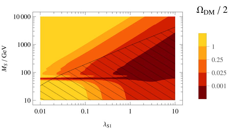
In this example, we reproduce the results of [10] where the standard model (SM) is extended by a real scalar gauge-singlet $S$ that is supposed to be the single component of the dark matter (DM) relic density. To this end, we make use of the $\mathbb{Z}_{3}$ symmetric dark matter model [11] implemented in micrOMEGAs3.6.9.2 [12, 13] to calculate the dark matter relic density $\Omega_{DM}$ (“Omega_DM”) and dark-matter-nucleon cross-sections $\sigma_{S,N}$ (“sigma_S_N”) for $N=p,n$ (proton and neutron) as a function of the scalar coupling $\lambda_{S1}$ (“laS1”) to the Higgs boson and the dark matter particle mass $M_{S}$ (“MS”).

Note that the model as implemented in micrOMEGAs actually includes a complex scalar gauge-singlet instead of a real one, so we have to divide $\Omega_{DM}$ by two to directly compare it with [10]. To obtain the correct limit in all other aspects, the other scalar couplings of the $\mathbb{Z}_{3}$ model will be set to zero and the surplus particles will be decoupled by setting their masses to 1000 TeV. The Higgs boson mass will be fixed to 125.7 GeV.

For the calculation, we will use a slightly modified version of the code included in the micrOMEGAs package. The relevant binary (“main-Z3MH”) expects a “data.par” input file given as command line argument, which can be written as the template file “data.par.template”:

⬇

Mh 125.7

Mdm1 $MS

Mdm2 1.0e6

MHC 1.0e6

muppS 0

la3 0

la2 0

laS 0

laS1 $laS1

laS2 0

laS21 0

sinDm 0

Since micrOMEGAs prints its results to the console, we choose to use “SimpleProcessor”. Looking at the usual output of the code, we see that $\Omega_{DM}$ is the $4$’th number printed and the DM-nucleon cross-sections are given by the $8$’th and $4$’th number from the back (with a variable number of values in between).

The scan definition file “ScalarDM.scan” is then given by:

⬇

[setup]

mode = scan

template = data.par.template

point_processor = processors/SimpleProcessor.py

[SimpleProcessor]

program = main-Z3MH

data_values = values[3], values[-8], values[-4]

[parameter_space]

par_names = laS1, MS

data_names = Omega_DM, sigma_S_p, sigma_S_n

par_laS1 = interval(0.01, 10) with count=200, distribution=log

par_MS = interval(10, 10000) with count=200, distribution=log

We will first test our scan definition by launching T3PS in “test” mode by running

⬇

$ t3ps--mode test ScalarDM.scan

As always T3PS will first show an overview of the settings as derived from the scan definition file before any calculation is run. It will then ask the user directly for parameter values of points that shall be calculated leading to console interactions like the following (user input in bold):

⬇

[…]

# Enter point (format: laS1, MS; as numbers or ’random’):

> 0.5, 1100

# Parameters:

laS1 = 0.5, MS = 1100.0

# Calculation done after: 0.041191 s

# Data:

-------------------------------------------

Omega_DM : 0.111 | sigma_S_p: 1.779e-09

sigma_S_n: 1.814e-09 | --- : ---

-------------------------------------------

# Output columns:

------------------------------------------------

1 : 0.5 | 2 : 1100.0 | 3 : 0.111

4 : 1.779e-09 | 5 : 1.814e-09 | ---: ---

------------------------------------------------

[…]

If all our test input points yield satisfying results, we can launch T3PS in its configured mode using

⬇

$ t3psScalarDM.scan

and after some cross-checks by T3PS with the user, the scan is performed without much interaction and saved to the file “ScalarDM.scan.data” (among others).

This file can then be read and turned into plots using the following code sketch for Mathematica

⬇

points = Import["ScalarDM.scan.data", "Table"];

ListContourPlot[points[[All, {1,2,3}]]]

and for gnuplot

⬇

splot "ScalarDM.scan.data" using 1:2:3

(both examples for $\Omega_{DM}$ over $\lambda_{S1}$-$M_{S}$ plots). The resulting contour plot for the DM relic density is shown in fig. 2. As we can see, a comparison with fig. 2b in [10] yields only very small (and expected due to e.g. a different Higgs boson mass) differences.

Figure 2: The DM relic density $\Omega_{DM}$ as function of the two scalar DM model parameters. The hatched region is excluded by $\sigma_{S,p}$ being above the 90% CL bound as provided by the LUX experiment [14] and obtained from DMTools [15]. Note that for better comparison with [10], the relic density has been divided by two.

7.2 Lepton Mixing and Charged Lepton Corrections

In this example scan, we will demonstrate the “optimize” and “mcmc” scan modes. For this, we choose to investigate how well the present global fit of the PMNS matrix can be reproduced by tribimaximal mixing in the neutrino sector and charged lepton mixing strictly between the first two generations.

Since the computation for this is relatively easy, we write our own point processor file “fit_pmns.py”:

⬇

# import SciPy for nicer matrix usage

import scipy as sp

# import some more mathematical functions

from math import sin, cos, sqrt

from cmath import exp

def main(template_file, pars, vars):

# we can also access pars and vars by name here

theta12e = pars.theta12e

s12e, c12e = sin(theta12e), cos(theta12e)

delta12e = pars.delta12e

UTBM = sp.matrix([

[-sqrt(2/3.), 1/sqrt(3), 0],

[ 1/sqrt(6), 1/sqrt(3), 1/sqrt(2)],

[ 1/sqrt(6), 1/sqrt(3), -1/sqrt(2)]

])

Ue = sp.matrix([

[c12e, s12e * exp(1j * delta12e), 0],

[-s12e * exp(-1j * delta12e), c12e, 0],

[0, 0, 1]

])

# m.H = hermitian transpose of m

UPMNS = Ue.H * UTBM

# indices are 0-based!

sin13 = abs(UPMNS[0,2])

tan12 = abs(UPMNS[0,1] / UPMNS[0,0])

tan23 = abs(UPMNS[1,2] / UPMNS[2,2])

sin12 = tan12 / sqrt(1 + tan12 ** 2)

sin23 = tan23 / sqrt(1 + tan23 ** 2)

return [sin12, sin23, sin13]

As one can see, the code simply multiplies the tribimaximal mixing matrix UTBM with the charged lepton mixing matrix Ue and extracts the $\sin$’s of the three mixing angles.

The scan definition file for finding the best fit point (using the 2014 NuFIT values [16] as target) is then given by (as file “ChargedLeptons_optimize.scan”):

⬇

[setup]

# do optimization with default population size

# (10*2 = 20 in this case)

mode = optimize

# use our custom processor

# (it uses no template file)

point_processor = fit_pmns.py

[parameter_space]

# two parameters that are angles in radians

# (only interested in first quadrant for theta)

par_names = theta12e, delta12e

par_theta12e = interval(0, 1.5707963267948966)

par_delta12e = interval(0, 3.141592653589793)

data_names = sin12, sin23, sin13

[algorithm]

# fit to "NuFIT Free Fluxes + RSBL"

# (use higher minimum for theta23)

chi_squared = (

((data.sin12 ** 2 - 0.304) / 0.012) ** 2 +

((data.sin23 ** 2 - 0.577) / 0.03) ** 2 +

((data.sin13 ** 2 - 0.0219) / 0.0010) ** 2

)

likelihood = -(%(chi_squared)s)

Note that, as introduced in sec. 3.1, the placeholder string “%(chi_squared)s” is replaced with the value of the directive chi_squared. Being interested in the probability distributions of our parameters, we also calculate those using the Markov chain Monte Carlo algorithm (mode “mcmc”) using the scan definition file “ChargedLeptons_mcmc.scan” (which extends the previous definition file using “@include”):

⬇

@include ChargedLeptons_optimize.scan

[setup]

# do MCMC analysis with chains containing 10000

# points each

mode = mcmc

unit_length = 10000

[parameter_space]

# amend parameters with step sizes

par_theta12e = interval(0, 1.5707963267948966) with mcmc_stepsize=0.003

par_delta12e = interval(0, 3.141592653589793) with mcmc_stepsize=0.04

[algorithm]

# switch from a chi^2 to a distribution function

likelihood = exp(-0.5 * (%(chi_squared)s))

Here, we used the information on the $\chi^{2}$ parabolas obtained from the “optimize” scan to get an estimate for the MCMC step sizes.

	best fit value	$1\sigma$ uncertainty
$\theta_{12}^{e}$ in ∘	12.07	${}^{+0.25}_{-0.31}$
$\delta_{12}^{e}$ in ∘	74.7	$\pm 5.1$
$\sin^{2}\theta_{12}^{\text{PMNS}}$	0.304	${}^{+0.12}_{-0.11}$
$\sin^{2}\theta_{23}^{\text{PMNS}}$	0.4888	${}^{+0.0006}_{-0.0004}$
$\sin^{2}\theta_{13}^{\text{PMNS}}$	0.0218	$\pm 0.0010$
$a$ in $10^{-5}$	1.36	${}^{+0.04}_{-0.03}$
$b$ in $10^{-4}$	1.26	$\pm 0.03$
$c$ in $10^{-4}$	5.881	${}^{+0.008}_{-0.007}$

Table 1: Statistical information obtained from the fit and MCMC analysis of charged lepton corrections to tribimaximal mixing. The Pearson correlation coefficient between the fitted parameters $\theta_{12}^{e}$ and $\delta_{12}^{e}$ is $0.05$ and the minimal $\chi^{2}$ is $8.64$. The correlation coefficients between $a$, $b$ and $c$ are $\rho_{ab}=-0.998$, $\rho_{ac}=0.82$ and $\rho_{bc}=-0.80$.

In a final step, we will use the obtained information on $\theta_{12}^{e}$ and values for the electron and muon Yukawa couplings $y_{e}$ and $y_{\mu}$ [17] to fit the parameters of a very simple flavor model. For simplicity, we neglect mixing to the third generation and only consider the first two generations. The relevant Yukawa coupling matrix is then given by

$$Y_{e}=\begin{pmatrix}0&b\\ a&c\end{pmatrix}\;,$$ (1)

which is defined to appear in the Lagrangian as $L_{i}(Y_{e})_{ij}e^{c}_{j}H_{d}$. The relevant equations $Y_{e}$ has to fulfill to reproduce the Yukawa couplings and the mixing angle are given by

$$|\det Y_{e}|=y_{e}\cdot y_{\mu}\;,\;||Y_{e}||^{2}=y_{e}^{2}+y_{\mu}^{2}\;,\;\left|\frac{b\cdot c}{a^{2}+c^{2}}\right|=\tan\theta_{12}^{e}\;,$$ (2)

where we used a zeroth order approximation in $y_{e}/y_{\mu}$ in the last equation and assumed all parameters to be real. Because the equation solving capabilities of standard Python are limited, we will again use the SciPy package. Since there is nothing else to calculate, we will omit the specification of a point processor and instead do the whole calculation using variables. The scan definition file “ChargedLeptons_matrixfit.scan”, which solves the relevant equations is then given by

⬇

[setup]

helper_modules = scipy.optimize:scipy.linalg

[parameter_space]

par_names = ye, ymu, theta12e

# numbers taken from arXiv:1306.6879

par_ye = normalvariate(2.8501e-6, 0.0022e-6)

par_ymu = normalvariate(6.0167e-4, 0.0044e-4)

# ... and previous scans

par_theta12e = normalvariate(0.211, 0.005)

var_names = a, b, c

Y_e = [[0, b], [a, c]]

var_a = remember(a_b_c=scipy.optimize.fsolve(

lambda (a, b, c): (

abs(scipy.linalg.det(%(Y_e)s)) -

(pars.ye * pars.ymu),

scipy.linalg.norm(%(Y_e)s) ** 2 -

(pars.ye ** 2 + pars.ymu ** 2),

abs(b * c / (a ** 2 + c ** 2)) -

tan(pars.theta12e)

),

(2e-5, 1e-4 , 6e-4)

))[0]

var_b = remember("a_b_c")[1]

var_c = remember("a_b_c")[2]

mode = scatter

point_count = 100000

As can be seen, we used the remember function to cache the result of numerical equation solving to avoid doing it again for each variable.

Finally, all resulting statistical information of all three parameter scans is summarized in tab. 1.

7.3 Maximal Higgs Mass in mSUGRA

In this example, we use the program SoftSUSY3.5.1 [18] to scan the mSUGRA parameter space and find the maximal possible Higgs boson mass over certain subspaces. The results are then compared with the ones found in the study in [19].

We start by writing a template file in SLHA format [7]. For the parameter scan, we intend to vary all 4+1 mSUGRA parameters and use the same input parameters as in [19]. Thus we arrive at a file named “mSUGRA.slha.template” with the following content:

⬇

Block MODSEL # Select model

1 1 # sugra

Block SMINPUTS # Standard Model inputs

1 1.279160000e+02 # alpha^(-1) SM MSbar(MZ)

2 1.166370000e-05 # G_Fermi

3 1.184000000e-01 # alpha_s(MZ) SM MSbar

4 9.119000000e+01 # MZ(pole)

5 4.190000000e+00 # mb(mb) SM MSbar

6 1.729000000e+02 # mtop(pole)

7 1.777000000e+00 # mtau(pole)

Block MINPAR # Input parameters

1 $m0 # m0

2 $m12 # m12

3 $tanBeta # tan beta at MZ, DRbar

4 $sign_mu # sign(mu)

5 $A0 # A0

Block SOFTSUSY # SOFTSUSY-specific

1 1.0e-03 # Numerical precision

2 0.0 # Quark mixing parameter

5 1.0 # 2-loop soft mass/trilinear RGEs

Note that we disabled quark and general flavor mixing to make the analysis of superpartner masses not unnecessarily complicated.

For the parameter scan, we write the following scan definition to a file with the name “HiggsMass_scatterscan.scan”:

⬇

[setup]

mode = scan

# use our template and the SLHAProcessor

template = mSUGRA.slha.template

point_processor = processors/SLHAProcessor.py

[SLHAProcessor]

# command line syntax as per SoftSUSY manual

program = softpoint.x leshouches < {template} > SLHASpectrum

slha_files = SLHASpectrum

# extract several masses from the spectrum file

# (for the PDG code meanings, see data_names)

slha_data = slha[0]["MASS"][25],

slha[0]["MASS"][1000022],slha[0]["MASS"][1000024],

slha[0]["MASS"][1000006],slha[0]["MASS"][2000006],

slha[0]["MASS"][1000021],

slha[0]["MASS"][1000001],slha[0]["MASS"][1000002],

slha[0]["MASS"][2000001],slha[0]["MASS"][2000002],

min([

slha[0]["MASS"][code]

for code in [1000012, 1000014, 1000016]

]),

slha[0]["MASS"][2000011],slha[0]["MASS"][2000013],

slha[0]["MASS"][1000015],slha[0]["MASS"][1000005]

[parameter_space]

# mSUGRA has 5 parameters:

par_names = m0, m12, A0, sign_mu, tanBeta

# scan over the following continuous ranges:

par_m0 = interval(50, 3000)

par_m12 = interval(50, 3000)

par_A0 = interval(-9000, 9000)

par_tanBeta = interval(1, 60)

# (except for the sign of mu of course)

par_sign_mu = -1, 1

# give names to all the masses

data_names = mh0,

mN1, mC1,

mstop1, mstop2,

msG,

msdL, msuL,

msdR, msuR,

msNu,

mseR, msMuR,

msTau1, msb

# impose three constraints

bound_count = 3

# MSUSY must be below 3 TeV

bound_0 = sqrt(data.mstop1 * data.mstop2) < 3000

# masses have to satisfy current PDG bounds

bound_1 = data.mN1 > 46

and (data.mC1 > 94 or pars.tanBeta > 40

or data.mC1-data.mN1 < 3)

and (data.msNu > 94 or pars.tanBeta > 40

or data.mseR-data.mN1 < 10)

and data.mseR > 107

and (data.msMuR > 94 or pars.tanBeta > 40

or data.msMuR-data.mN1 < 10)

and (data.msTau1 > 81.9

or data.msTau1-data.mN1 < 15)

and min(data.msuL, data.msdL, data.msuR,

data.msdR) > 1.11e3

and (data.msb > 89 or data.msb-data.mN1 < 8)

and (data.mstop1 > 95.7

or data.mstop1 - data.mN1 < 10)

and data.msG > 800

# the neutralino shall be the LSP

bound_2 = data.mN1 <= min(

data[i] for i in range(len(data)) if i != 0

)

# do a random scan

mode = scatter

point_count = 100000

As can be seen, we perform a “scatter” scan where we calculate $100000$ points taken at random from a set of continuous or discrete ranges. For the bounds, we stuck to the constraint $M_{\text{SUSY}}<3$ TeV as also imposed in [19] and used the bounds as given in [20] for the superpartner masses.

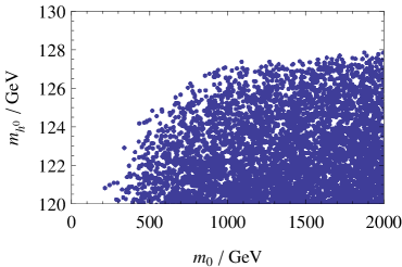
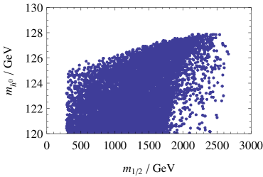
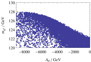
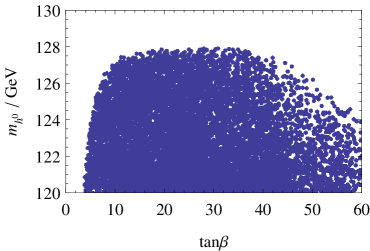
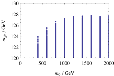
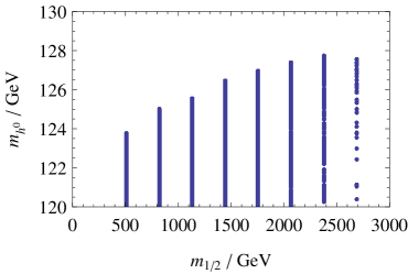
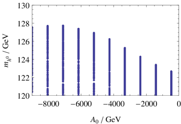
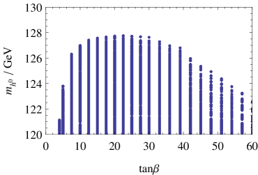
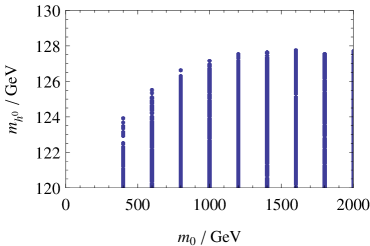
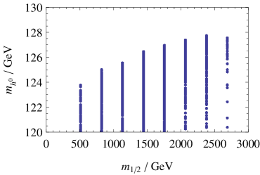
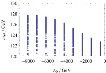
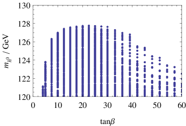
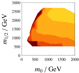
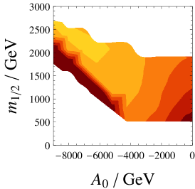
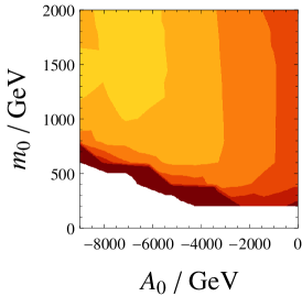
We then let T3PS run the parameter scan, which is complete after about 105 minutes (on a 3.4 GHz Intel i7 quad core processor). The resulting plots can be seen in fig. 3. A comparison with the analogous plots of [19] (fig. 3 a-d therein) shows that both have almost the same behavior with only minor differences that can be attributed to more rigorous constraints for the superpartner spectrum in [19].

As an additional refinement, one might be interested in the maximal Higgs boson mass over two-dimensional parameter subspaces instead of one-dimensional ones. This would involve binning the randomly distributed points appropriately in the respective plain. Instead, we go for an automatically binned strategy involving a discrete grid over which we scan our five mSUGRA parameters. The corresponding scan definition file “HiggsMass_gridscan.scan” only has a few lines:

⬇

@include HiggsMass_scatterscan.scan

[parameter_space]

mode = grid

par_m0 = interval(200, 2000) with count = 10

par_m12 = interval(200, 3000) with count = 10

par_A0 = interval(-9000, 9000) with count = 20

par_tanBeta = 1, 2,..., 5, 7.5,..., 30, 33,..., 60

Again after about 95 minutes (on the same 3.4 GHz Intel i7 quad core processor), T3PS has finished the scan. The resulting plots for one-dimensional subspaces are shown in fig. 4 with (as expected) good agreement with the previously obtained data set.

An additional feature of T3PS is the so called “explorer” mode. This mode is exactly designed for this sort of calculation, i.e. maximizing a given function over several different plains in parameter space. Adapting our grid scan to this mode is not complicated and yields the following scan definition file “HiggsMass_explorer.scan”:

⬇

@include HiggsMass_gridscan.scan

[setup]

mode = explorer

[algorithm]

# maximize the Higgs boson mass!

likelihood = data.mh0

min_likelihood = 118

# calculate maximal Higgs boson mass over several

# different planes (or lines)

projection_count = 7

projection_0 = pars.m0, pars.m0

projection_1 = pars.m12, pars.m12

projection_2 = pars.A0, pars.A0

projection_3 = pars.tanBeta, pars.tanBeta

projection_4 = pars.m0, pars.m12

projection_5 = pars.m0, pars.A0

projection_6 = pars.m12, pars.A0

# two (probably not very good) symmetries

symmetry_count = 2

# no dependence on sign of mu?

symmetry_0 = sign_mu: -pars.sign_mu

# no dependence on sign of A0?

symmetry_1 = 2: -pars[2]

# only do state one calculation

disabled_states = 2, 3

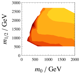
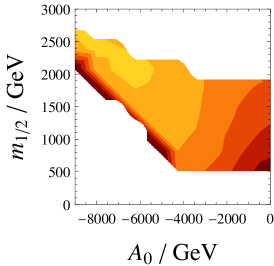
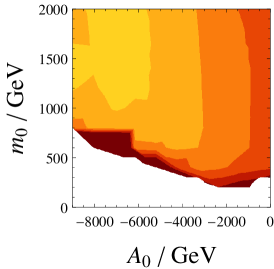
After running this scan for about 5 minutes, we find analogous plots to the two previous scans as shown in fig. 5. Additionally, we can compare plots of the maximal Higgs boson mass over some two-dimensional plains as shown in fig. 6. As can be seen, the differences are already very small compared to the calculation of the full parameter space grid.

Note that there are multiple ways to improve the data obtained using the “explorer” mode. For example, one can simply enable algorithm states two and three and let T3PS run longer. On the other hand, keeping in mind that in this example the starting points were chosen at random, one can also choose those more carefully. This can be done by hand using the “test” mode and consequently using the “.testdata” file as input or by running a scan in the “optimize” mode beforehand and thereby creating an already nearly optimal starting point set.

As final part of this example, we will compare the results obtained with SoftSUSY with what we would have gotten with SPheno3.3.3 [21, 22]. For demonstration purposes, we will make use of the manager-worker architecture, too. The content of the scan definition file “HiggsMass_recalc.scan” is then given by:

⬇

@include HiggsMass_explorer.scan

[setup]

mode = scan

workers = 127.0.0.1

authkey = HiggsMass_recalc

[SLHAProcessor]

program = SPheno {template} SLHASpectrum

[parameter_space]

mode = file

files = HiggsMass_explorer.scan.data

file_columns = m0, m12, A0, sign_mu, tanBeta, mh0

par_m0 = file.m0

par_m12 = file.m12

par_A0 = file.A0

par_sign_mu = file.sign_mu

par_tanBeta = file.tanBeta

[algorithm]

out_columns = pars.m0, pars.m12, pars.A0,

pars.sign_mu, pars.tanBeta, data.mh0 - file.mh0

Note that the used version of SPheno does not make use of exit codes to signal invalid parameters. However, it will write an incomplete SLHA spectrum file instead, which will lead to errors from SLHAProcessor due to a missing “MASS” block.

As can be seen, we use the parameter space mode “file”. This means that the parameter space is taken directly from the points contained in the output file of the “explorer” scan. The parameter values are simply taken one-to-one from the data file. The out_columns directive causes that only the specified values are saved to the result file instead of all parameter and calculated data values. Finally, the worker instance of T3PS can be launched using

⬇

$ t3psHiggsMass_recalc.scan --mode worker

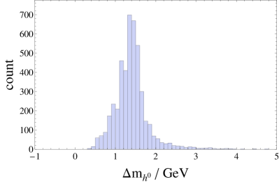
As shown in fig. 7, both codes only differ by about $1.5$ GeV in their Higgs mass result.

Figure 3: Value of the Higgs boson mass $m_{h^{0}}$ as function of each of the four continuous mSUGRA parameters (marginalizing over the others each time) as found in the scattering scan. No further constraints than the ones in the scan definition file were applied.

Figure 4: Value of the Higgs boson mass $m_{h^{0}}$ as function of each of the four continuous mSUGRA parameters (marginalizing over the others each time) as found in the grid scan. No further constraints than the ones in the scan definition file were applied.

Figure 5: Value of the Higgs boson mass $m_{h^{0}}$ as function of each of the four continuous mSUGRA parameters (marginalizing over the others each time) as found in the “explorer” scan. No further constraints than the ones in the scan definition file were applied.

Figure 6: Maximal value of the Higgs boson mass $m_{h^{0}}$ as function of the four continuous mSUGRA parameters (marginalizing over the others) as found in the grid (upper) and “explorer” (lower) scan.

Figure 7: Difference between the Higgs mass as calculated by the codes SoftSUSY and SPheno for the points found in the “explorer” scan.

Appendix A Implemented Algorithms

A.1 Markov Chain Monte Carlo

The implemented Metropolis-Hastings algorithm [3, 4] – starting from a point p0 – can be sketched as:

⬇

While count_points < requested_count_points:

p1 = new_random_point_around(p0, stepsizes)

If p1 is excluded by prior:

stay_count = stay_count + 1

Redo

Else If p1 is excluded by constraints:

stay_count = stay_count + 1

Redo

End

L1 = L(p1) * prior(p1)

L0 = L(p0) * prior(p0)

a = random_uniform(0, 1)

If a < min(L1 / L0 * q(p0, p1) / q(p1, p0), 1):

Save p0 (with stay count)

p0 = p1

stay_count = 1

count_points = count_points + 1

Else:

stay_count = stay_count + 1

End

End

where L(p) is the propagation likelihood value for the point p and q(p1, p0) is the proposal density (up to normalization) for the point p1 around p0. In the case of flat prior probability, L corresponds to the target probability distribution function (up to normalization). For the relevant scan definition directives, see sec. 3.5.

A.2 Optimization using Differential Evolution

The implementation of the differential evolution algorithm [5] as applied to a fitness function f can be sketched as:

⬇

While waiting $\leq$ max_waiting_time:

For each x in population:

a, b, c = Find three random points

in population with

a $\neq$ b $\neq$ c $\neq$ a and a, b, c $\neq$ x

xs = a + S * (b - c)

For i from 1 to count_dimensions:

r = random_uniform(0, 1)

If r < rho:

y[i] = x[i]

Else:

y[i] = xs[i]

End

End

If f(y) > f(x):

Replace x -> y in population

End

End

new = max{f(x) for x in new population}

old = max{f(x) for x in old population}

If abs(new - old) < eps + eps_rel * old:

waiting = waiting + 1

Else:

waiting = 0

End

End

where S $\in[0,2]$ is the differential weight (default: 0.6), rho $\in[0,1]$ is the crossover probability (default: 0.5), eps is the absolute waiting threshold (default: 0) and eps_rel is the relative waiting threshold (default: $10^{-8}$ for double precision) – the population size defaults to $10$ times the number of parameters with at least two possible values. For more information on the choice of these algorithm parameters, see e.g. [23]. For the relevant scan definition directives, see sec. 3.6.

Note that, after the last iteration, one has to extract the point with highest fitness value from the last population.

A.3 Swarm-like Explorative Optimization

Each iteration of the algorithm starting from a known point set $S$ can be sketched as:

⬇

If projections defined and state < 3:

For each projection in projections:

For each p in $S$:

If state > 1 or p $\notin$ boundary($S$):

Next

End

x, y, z = projected_coordinates(

projection, p

)

If z > z_max(x, y):

p_max(x, y) = p

z_max(x, y) = z

End

End

If state = 1:

For each x, y in projected_plain:

Add neighbors(best_point[x, y]) to $\mathcal{P}$

For dx, dy in simple_orbit(0):

Add points from line segment

[p_max(x, y) p_max(x+dx, y+dy)]

to $\mathcal{P}$

Add points encountered by extending

previous line segment to $\mathcal{P}$

Apply symmetries to p_max(x, y)

and add result to $\mathcal{P}$

End

End

End

End

Else:

For each p in $S$:

If $\exists$ n with n $\in$ neighbors(p) and n $\notin S$

Add p to boundary bin $\mathcal{B}_{i}$ according to L(p)

End

End

$\mathcal{B}$ = highest likelihood, non empty $\mathcal{B}_{i}$

For each p in $\mathcal{B}$:

Add neighbors(p) to $\mathcal{P}$

End

End

If $\mathcal{P}$ is empty:

If state < 3:

state = state + 1

End

Else:

For each p in $\mathcal{P}\setminus S$:

Process p and add it to $S$

End

If projections defined:

state = 1

End

End

$\mathcal{P}$ = {}

where L(p) is the likelihood function value for the point p. For the relevant scan definition directives, see sec. 3.7.

References

- [1] Wolfram Research Inc., Mathematica version 7.0, Champaign, Illinois (2008).
- [2] T. Williams, C. Kelley, many others, Gnuplot 4.4: an interactive plotting program, http://gnuplot.sourceforge.net/ (March 2010).
-
[3]
N. Metropolis, A. W. Rosenbluth, M. N. Rosenbluth, A. H. Teller, E. Teller,
Equation of state calculations by fast computing machines, The Journal of
Chemical Physics 21 (6) (1953) 1087–1092.
doi:http://dx.doi.org/10.1063/1.1699114.
URL http://scitation.aip.org/content/aip/journal/jcp/21/6/1%0.1063/1.1699114 -
[4]
W. K. Hastings, Monte carlo sampling
methods using markov chains and their applications, Biometrika 57 (1) (1970)
pp. 97–109.
URL http://www.jstor.org/stable/2334940 -
[5]
R. Storn, K. Price,
Differential evolution - a
simple and efficient heuristic for global optimization over continuous
spaces, Journal of Global Optimization 11 (4) (1997) 341–359.
doi:10.1023/A:1008202821328.
URL http://dx.doi.org/10.1023/A%3A1008202821328 - [6] Python Software Foundation, ConfigParser - Configuration file parser, [http://docs.python.org/2/library/configparser.html] [Online; accessed 2014-10-09] (2014).
- [7] P. Z. Skands, B. Allanach, H. Baer, C. Balazs, G. Belanger, et al., SUSY Les Houches accord: Interfacing SUSY spectrum calculators, decay packages, and event generators, JHEP 0407 (2004) 036. arXiv:hep-ph/0311123, doi:10.1088/1126-6708/2004/07/036.
- [8] P. Bechtle, O. Brein, S. Heinemeyer, O. St l, T. Stefaniak, et al., : Improved Tests of Extended Higgs Sectors against Exclusion Bounds from LEP, the Tevatron and the LHC, Eur.Phys.J. C74 (2014) 2693. arXiv:1311.0055, doi:10.1140/epjc/s10052-013-2693-2.
- [9] F. Mahmoudi, S. Heinemeyer, A. Arbey, A. Bharucha, T. Goto, et al., Flavour Les Houches Accord: Interfacing Flavour related Codes, Comput.Phys.Commun. 183 (2012) 285–298. arXiv:1008.0762, doi:10.1016/j.cpc.2011.10.006.
- [10] J. McDonald, Gauge singlet scalars as cold dark matter, Phys.Rev. D50 (1994) 3637–3649. arXiv:hep-ph/0702143, doi:10.1103/PhysRevD.50.3637.
- [11] G. Belanger, K. Kannike, A. Pukhov, M. Raidal, Impact of semi-annihilations on dark matter phenomenology - an example of symmetric scalar dark matter, JCAP 1204 (2012) 010. arXiv:1202.2962, doi:10.1088/1475-7516/2012/04/010.
- [12] G. Belanger, F. Boudjema, A. Pukhov, A. Semenov, MicrOMEGAs: A Program for calculating the relic density in the MSSM, Comput.Phys.Commun. 149 (2002) 103–120. arXiv:hep-ph/0112278, doi:10.1016/S0010-4655(02)00596-9.
- [13] G. Belanger, F. Boudjema, A. Pukhov, A. Semenov, micrOMEGAs_3: A program for calculating dark matter observables, Comput.Phys.Commun. 185 (2014) 960–985. arXiv:1305.0237, doi:10.1016/j.cpc.2013.10.016.
- [14] D. Akerib, et al., First results from the LUX dark matter experiment at the Sanford Underground Research Facility, Phys.Rev.Lett. 112 (2014) 091303. arXiv:1310.8214, doi:10.1103/PhysRevLett.112.091303.
- [15] DMTools, [http://dmtools.brown.edu:8080/] [Online; accessed 2014-09-05].
- [16] M. Gonzalez-Garcia, M. Maltoni, J. Salvado, T. Schwetz, Global fit to three neutrino mixing: critical look at present precision, JHEP 1212 (2012) 123. arXiv:1209.3023, doi:10.1007/JHEP12(2012)123.
- [17] S. Antusch, V. Maurer, Running quark and lepton parameters at various scales, JHEP 1311 (2013) 115. arXiv:1306.6879, doi:10.1007/JHEP11(2013)115.
- [18] B. Allanach, SOFTSUSY: a program for calculating supersymmetric spectra, Comput.Phys.Commun. 143 (2002) 305–331. arXiv:hep-ph/0104145, doi:10.1016/S0010-4655(01)00460-X.
- [19] A. Arbey, M. Battaglia, A. Djouadi, F. Mahmoudi, J. Quevillon, Implications of a 125 GeV Higgs for supersymmetric models, Phys.Lett. B708 (2012) 162–169. arXiv:1112.3028, doi:10.1016/j.physletb.2012.01.053.
- [20] K. A. Olive, et al., Review of Particle Physics, Chin. Phys. C38 (2014) 090001.
- [21] W. Porod, F. Staub, SPheno 3.1: Extensions including flavour, CP-phases and models beyond the MSSM, Comput.Phys.Commun. 183 (2012) 2458–2469. arXiv:1104.1573, doi:10.1016/j.cpc.2012.05.021.
- [22] W. Porod, SPheno, a program for calculating supersymmetric spectra, SUSY particle decays and SUSY particle production at e+ e- colliders, Comput.Phys.Commun. 153 (2003) 275–315. arXiv:hep-ph/0301101, doi:10.1016/S0010-4655(03)00222-4.
- [23] R. Storn, On the usage of differential evolution for function optimization, in: Fuzzy Information Processing Society, 1996. NAFIPS., 1996 Biennial Conference of the North American, 1996, pp. 519–523. doi:10.1109/NAFIPS.1996.534789.