Projection-based model reduction for contact problems

Abstract

To be feasible for computationally intensive applications such as parametric studies, optimization and control design, large-scale finite element analysis requires model order reduction. This is particularly true in nonlinear settings that tend to dramatically increase computational complexity. Although significant progress has been achieved in the development of computational approaches for the reduction of nonlinear computational mechanics models, addressing the issue of contact remains a major hurdle. To this effect, this paper introduces a projection-based model reduction approach for both static and dynamic contact problems. It features the application of a non-negative matrix factorization scheme to the construction of a positive reduced-order basis for the contact forces, and a greedy sampling algorithm coupled with an error indicator for achieving robustness with respect to model parameter variations. The proposed approach is successfully demonstrated for the reduction of several two-dimensional, simple, but representative contact and self contact computational models.

1 Introduction

The nonlinear finite element (FE) analysis (FEA) of large-scale systems often requires prohibitively large computational resources. These are typically prescribed by the fine discretization of the computational domain that leads to a large number of degrees of freedom (dofs) in the system, as well as, in the case of dynamic analysis, the potentially large number of time-steps needed to accurately describe the evolution of the system.

Projection-based model order reduction (MOR) techniques alleviate the first issue by restricting the solution space to a smaller subspace, thereby reducing the number of dofs. While many approaches have already been developed for the efficient reduction of linear computational models [1, 2, 3, 4], three main strategies have been explored so far for efficiently reducing nonlinear computational models. The first one is based on linearization techniques [5, 6]. The second one is based on the notion of pre-computations [7, 8] but is limited to polynomial nonlinearities. The third strategy relies on the concept of hyper-reduction — that is, the approximation of the reduced operators underlying a nonlinear reduced-order model (ROM) by a scalable numerical technique based on a reduced computational domain [9, 10, 11, 12, 13, 14, 15]. While several hyper-reduction techniques have been proposed in the literature, two of them have been designed specifically for the nonlinear FEA of structural and solid mechanics problems: The a priori hyper-reduction method [9], and the Energy Conserving Sampling and Weighting method [10, 14, 16]. Nevertheless, contact problems remain a major hurdle for nonlinear model reduction in the context of structural analysis. This is because, among other things, contact problems are characterized by inequality constraints that complicate the reduction process.

Most if not all (nonlinear) computational contact methods proceed in two steps. The first one focuses on contact detection — that is, the identification of nodes, edges, and/or faces of the computational model that should be in contact. The second step focuses on contact enforcement — that is, the satisfaction of the contact constraints defined by physical laws such as non-penetration and frictional behavior. In practice, the aforementioned constraints are enforced using one of three popular approaches: The penalty method, the Lagrange multiplier method, or the augmented Lagrange multiplier method [17, 18]. Attention is focused in this paper on the case of the Lagrange multipler method (or its augmented version).

For large-scale nonlinear dynamical systems, proper orthogonal decomposition (POD) [19] is the method of choice for generating the reduced-order basis (ROB) needed for constructing a ROM. It proceeds by collecting solution snapshots during a training procedure, then compressing them using the singular value decomposition (SVD) method. The resulting ROB minimizes the projection error of the snapshots. However, when the Lagrange multiplier method is chosen for enforcing contact constraints, reducing the contact forces — or equivalently, the Lagrange multipliers — requires special care because the reduced multipliers must have a positive sign. A ROB for these dual variables based on SVD would not enforce this positivity requirement a priori. For this reason, it is proposed in this paper to reduce positive quantities such as contact forces or Lagrange multipliers using a positive counterpart of the SVD method known as the non-negative matrix factorization (NNMF) method. Introduced first in the context of image compression [20], this method builds low-rank positive factors that approximate a given non-negative matrix. Here, it is shown that the proposed usage of NNMF results in the construction of a ROB that can accurately represent the Lagrange multipliers and lead to the effective reduction of contact computational models.

In [21, 22], the authors have addressed similar issues by constructing a ROB for the Lagrange multipliers using a positive linear combination of pre-computed snapshots of these dual variables. For time-dependent problems, this approach can rapidly become impractical as it can lead to the construction of a ROB of very large dimension. In this work, NNMF provides a natural procedure for optimally compressing a potentially large number of snapshots of the dual variables and constructing a small dimensional ROB for approximating them.

A more generic model reduction issue is the robustness of a ROM with respect to variations of the model parameters. Indeed, a ROM is truly useful when it can be used as a surrogate of the underlying high-dimensional model (HDM) for parameter values that may be different from those sampled for the purpose of constructing a ROB. Contact problems can be particularly sensitive to parameter variations, for example, when the contact areas are very sensitive to such variations. A popular approach for constructing a ROM that is valid in a large region of the model parameter domain is to couple a greedy approach with one or several a posteriori error estimators [23, 24, 25, 26] in order to effectively sample the parameter domain for computing solution snapshots and constructing a ROB. Such an approach constructs increasingly accurate ROMs by detecting locations in the model parameter domain where the errors associated with the ROM are the largest. The associated HDM is subsequently reconstructed at the identified worst-error parameter values and solution snapshots are computed and stored. Then, the ROB — and therefore ROM — is updated based on these additional snapshots, thereby reducing drastically the error(s) for the newly sampled parameter values. This procedure terminates whenever the estimated ROM error(s) is (are) below a specified tolerance throughout the model parameter domain of interest. It leads to a ROM that remains accurate away from the training configurations. Therefore in this work, a greedy approach is also developed to construct both primal and dual ROBs that are robust in a given model parameter domain. Specifically, the greedy approach developed in this paper relies on the definition of an error indicator for the contact problem, and successive updates of both primal and dual ROBs computed using SVD and NNMF, respectively, are performed.

The remainder of this paper is organized as follows. The notation adopted in this paper is presented in Section 2. The considered family of contact problems is derived in Section 3. The proposed model reduction procedure for contact problems is described in Section 4. This procedure is applied in Section 5 to the reduction of three different contact problems. Finally, conclusions are offered in Section 6.

2 Notation

Throughout this paper, matrices are denoted by bold capitals (ex. $\bm{A}$), vectors by bold lower cases (ex. $\bm{a}$), and subscripts identify rows and columns (ex. $A_{i,j}$ is the entry of $\bm{A}$ located in the $i$-th row and $j$-th column of this matrix).

$\bm{A}^{+}$ denotes the Moore-Penrose pseudo-inverse of the matrix $\bm{A}$.

$\bm{I}_{N}$ identifies the identity matrix of size $N$ and $\bm{0}$ identifies a matrix of zeros. $\bm{1}_{N}$ identifies the vector of dimension $N$ whose entries are all ones.

For two matrices $\bm{A}$ and $\bm{B}$ of equal dimension $M\times N$, the Hadamard product $\bm{A}\odot\bm{B}$ is the matrix of the same dimension whose entries are given by

$$\left(\bm{A}\odot\bm{B}\right)_{i,j}=A_{i,j}\cdot B_{i,j}$$ (1)

A discretized variable $\bm{u}\in\mathbb{R}^{N}$ at time-step $n\in\mathbb{N}$ is identified by a superscript as $\bm{u}^{n}\in\mathbb{R}^{N}$.

The standard Euclidean norm of a vector $\bm{x}\in\mathbb{R}^{N}$ and the Frobenius norm of a matrix $\bm{A}\in\mathbb{R}^{M\times N}$ are denoted by $\left\|\bm{x}\right\|_{2}$ and $\left\|\bm{A}\right\|_{F}$, respectively, and defined as follows

$$\left\|\bm{x}\right\|_{2}=\left({\sum\limits_{i=1}^{N}{x_{i}^{2}}}\right)^{\tfrac{1}{2}},\quad\left\|\bm{A}\right\|_{F}=\left({\sum\limits_{i=1}^{M}{\sum\limits_{j=1}^{N}{A_{i,j}^{2}}}}\right)^{\tfrac{1}{2}}.$$ (2)

Finally, the negative part of a real number $x$ is defined as $[x]_{-}:=\min(x,0)$ and that of a vector $\bm{x}\in\mathbb{R}^{N}$ is defined as $[\bm{x}]_{-}=\left[[x_{i}]_{-}\right]$.

3 Model contact problem

The main issue addressed in this paper is that of how to reduce the dual Lagrange multipliers introduced in a solution process for enforcing the inequality constraints governing a static or dynamic contact problem. For this reason, and for the sake of clarity, attention is focused here on a model contact problem where the individual bodies in contact (for example, see Fig. 1) have linear material and kinematic behaviors. The reduction of the primal displacement solution in the presence of material nonlinearities and/or large displacements and rotations raises independent issues that have already been addressed elsewhere in the literature, for example, in  [14, 16, 13, 12]. Furthermore, for simplicity and without any loss of generality, only the case of a frictionless, adhesive-free normal contact is considered, and all body problems are assumed to be undamped and semi-discretized on uniform matching meshes.

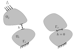
Figure 1: Illustration of a generic two-body contact problem.

Using the modeling assumptions stated above, the FE semi-discretization of a dynamic $N_{\Omega}$-body contact problem can be written in matrix form as

$$\bm{M}\ddot{\bm{u}}+\bm{K}\bm{u} = \bm{f}+\bm{B}^{\rm T}\bm{\lambda}$$

$$\bm{B}\bm{u}-\bm{c} \geq \bm{0}$$

$$\bm{u}(0) = \bm{u}_{0}$$

$$\dot{\bm{u}}(0) = \dot{\bm{u}}_{0}$$ (3)

where a dot designates a time derivative, the first semi-discrete equation expresses the dynamic equilibrium of $N_{\Omega}$ given (flexible) bodies, the inequality constraint derives from the semi-discretization of the Hertz-Signorini-Moreau contact conditions that coincide with the Karush-Kuhn-Tucker (KKT) complementary conditions in the theory of optimization [18], and the last two equations result from the semi-discretization of the initial conditions. In Eq. (3) above, $\bm{M}\in\mathbb{R}^{N\times N}$ and $\bm{K}\in\mathbb{R}^{N\times N}$, where $N$ denotes the total number of primal dofs, are constant symmetric positive definite or semi-definite block diagonal mass and stiffness matrices, $\bm{u}=\bm{u}(t)\in\mathbb{R}^{N}$ is a semi-discrete displacement vector and $t$ denotes time, $\bm{f}=\bm{f}(t)\in\mathbb{R}^{N}$ is a semi-discrete force vector, $\bm{B}\in\mathbb{R}^{N_{\lambda}\times N}$, where $N_{\lambda}$ denotes the total number of potentially active contact inequalities, is a signed boolean matrix which extracts from $\bm{u}$ the pairs of dof governed by a contact condition, $\bm{c}$ is the vector of initial clearances, and $\bm{\lambda}$ is the vector of semi-discrete Lagrange multipliers.

Specifically, $\bm{M}$, $\bm{K}$, $\bm{u}$, $\bm{B}$, $\bm{\lambda}$, and $\bm{f}$ can be written as

$$\bm{M} = \begin{bmatrix}\bm{M}_{1}&\bm{0}&\cdots&\bm{0}\\ \bm{0}&\bm{M}_{2}&\cdots&\bm{0}\\ \vdots&\vdots&\ddots&\vdots\\ \bm{0}&\cdots&\cdots&\bm{M}_{N_{\Omega}}\end{bmatrix},\quad\bm{K}=\begin{bmatrix}\bm{K}_{1}&\bm{0}&\cdots&\bm{0}\\ \bm{0}&\bm{K}_{2}&\cdots&\bm{0}\\ \vdots&\vdots&\ddots&\vdots\\ \bm{0}&\cdots&\cdots&\bm{K}_{N_{\Omega}}\end{bmatrix},\quad\bm{u}=\begin{bmatrix}\bm{u}_{1}\\ \bm{u}_{2}\\ \vdots\\ \bm{u}_{N_{\Omega}}\end{bmatrix}$$

$$\bm{B} = \begin{bmatrix}\bm{B}_{1}&\bm{B_{2}}&\cdots&\bm{B}_{N_{\Omega}}\end{bmatrix},\quad\bm{\lambda}=\begin{bmatrix}\bm{\lambda}_{1}\\ \bm{\lambda}_{2}\\ \vdots\\ \bm{\lambda}_{N_{\Omega}}\end{bmatrix},\quad\bm{f}=\begin{bmatrix}\bm{f}_{1}\\ \bm{f}_{2}\\ \vdots\\ \bm{f}_{N_{\Omega}}\end{bmatrix}$$ (4)

where the subscript $i=1,2,\cdots,N_{\Omega}$ designates the body $\Omega_{i}$.

Again, for simplicity and without any loss of generality, an implicit time-discretization is assumed in the dynamic case so that solving both static and dynamic contact problems can be formulated as

$$\begin{split}(\bm{u}^{n},\bm{\lambda}^{n})&=\operatorname*{argmin}_{\bm{v}\in{\mathbb{R}}^{N},~{}\bm{\mu}\in{\mathbb{R}}^{{+}^{N_{\lambda}}}}\frac{1}{2}{\bm{v}}^{\rm T}\bm{A}{\bm{v}}-{\bm{v}}^{\rm T}\bm{b}^{n}-{\bm{\mu}}^{\rm T}(\bm{B}\bm{v}-\bm{c})\end{split}$$ (5)

where $T$ designates the transpose operation, the superscript $n$ designates the $n$-th time-step $t_{n}$, $t_{0}=0<t_{1}<\cdots<t_{n}<\cdots<t_{N_{t}}=\mathcal{T}$ is a discretization of $[0,\mathcal{T}]$ into $N_{t}+1$ time-points, $\bm{A}\in{\mathbb{R}}^{N\times N}$ is the block diagonal matrix containing for each body its mass and stiffness matrices scaled according to the chosen time-integration algorithm and selected time-stepping strategy, $\bm{b}\in\mathbb{R}^{N}$ contains for each body the right-hand side vector arising from the implicit time-discretization of the dynamic semi-discrete equations of equilibrium governing this body, and $\bm{\lambda}\geq\bm{0}$. In the static case, the superscript $n$ is dropped, $\bm{A}=\bm{K}$, and $\bm{b}=\bm{f}$.

4 Model reduction

4.1 Galerkin projection

For the model contact problem described above, the standard Galerkin projection-based MOR method is appropriate. In this method, the primal and dual components of the solution are approximated in two reduced subspaces represented here by two pre-computed ROBs $\bm{U}\in\mathbb{R}^{N\times p}$ and $\bm{U}_{\lambda}\in\mathbb{R}^{N_{\lambda}\times p_{\lambda}}$, respectively. This can be written as

$$\bm{u}^{n}(\bm{\gamma})\approx\bm{U}\bm{u}_{r}^{n}(\bm{\gamma}),\quad\bm{\lambda}^{n}(\bm{\gamma})\approx\bm{U}_{\lambda}\bm{\lambda}_{r}^{n}(\bm{\gamma})$$ (6)

where $\bm{u}_{r}\in\mathbb{R}^{p}$ and $\bm{\lambda}_{r}\in\mathbb{R}^{p_{\lambda}}$ are the generalized coordinates of the reduced displacement and Lagrange multiplier solutions, respectively, and $\bm{\gamma}\in\mathcal{D}\subset\mathbb{R}^{m}$ is a vector of $m$ parameters of the contact problem of interest. Inserting the above two approximations in the saddle point problem (5) gives

$$\begin{split}(\bm{u}_{r}^{n},\bm{\lambda}_{r}^{n})&=\operatorname*{argmin}_{\bm{v}_{r}\in\mathbb{R}^{p},~{}\bm{\mu}_{r}\in\mathbb{R}^{{+}^{p_{\lambda}}}}\frac{1}{2}{\bm{v}_{r}}^{\rm T}\bm{A}_{r}{\bm{v}_{r}}-{\bm{v}_{r}}^{\rm T}\bm{b}_{r}-{\bm{\mu}_{r}}^{\rm T}(\bm{B}_{r}\bm{v}_{r}-\bm{c}_{r})\end{split}$$ (7)

where

$\bm{A}_{r}:=\bm{U}^{\rm T}\bm{A}\bm{U}\in\mathbb{R}^{p\times p}$, $\bm{b}_{r}^{n}:=\bm{U}^{T}\bm{b}^{n}\in\mathbb{R}^{p}$, $\bm{B}_{r}:=\bm{U}_{\lambda}^{T}\bm{B}\bm{U}\in\mathbb{R}^{p_{\lambda}\times p}$, and $\bm{c}_{r}:=\bm{U}_{\lambda}^{\rm T}\bm{c}\in\mathbb{R}^{p_{\lambda}}$.

To ensure the non-penetration condition in the contact ROM, the reduced vector of Lagrange multipliers must be non-negative — that is, $\bm{U}_{\lambda}\bm{\lambda}_{r}^{n}\geq\bm{0}$. The approach proposed in Section 4.3 for satisfying this requirement is to construct a non-negative ROB $\bm{U}_{\lambda}\geq\bm{0}$. Indeed, since the solution of the contact problem formulated using the contact ROM delivers a positive vector of generalized Lagrange multiplier coordinates $\bm{\lambda}_{r}\geq 0$, $\bm{U}_{\lambda}\geq\bm{0}$ guarantees in this case that $\bm{U}_{\lambda}\bm{\lambda}_{r}\geq\bm{0}$.

Algorithm 1 below outlines the Galerkin projection-based MOR method proposed in this paper for solving the contact problem (5). To this effect, note that in general, it is feasible to compute the reduced vector $\bm{b}_{r}^{n}$ online. Specifically, this can be achieved by pre-computing some relevant small-size quantities offline. For example, consider the case where the prescribed, time-dependent force vector can be decomposed as $\bm{f}(t)=\bm{L}g(t)$, where $\bm{L}\in\mathbb{R}^{N}$ describes the time-invariant spatial distribution of $\bm{f}$ and $g(t)\in\mathbb{R}$ describes its temporal evolution. If time-discretization is performed using the midpoint rule, $\bm{b}_{r}^{n}=\bm{M}_{r}\bm{u}_{r}^{n}+(\Delta t/2)\bm{M}_{r}\dot{\bm{u}}_{r}^{n}+(\Delta t^{2}/4)\bm{U}^{T}\bm{L}g(t_{n+1/2})$, where $\Delta t$ is the computational time-step. In this case, $\bm{b}_{r}^{n}$ can be efficiently computed at each time-step by pre-computing once for all the quantity $(\Delta t^{2}/4)\bm{U}^{T}\bm{L}$.

input : Reduced quantities $\bm{A}_{r}$, $\bm{B}_{r}$, $\bm{c}_{r}$, $\bm{u}_{r}^{0}$, and $\dot{\bm{u}}_{r}^{0}$

output : Generalized coordinates $\{\bm{u}_{r}^{n}\}_{n=1}^{N_{t}}$, $\{\bm{\lambda}_{r}^{n}\}_{n=1}^{N_{t}}$

1 for $n=1,2,\ldots,N_{t}$ do

2       Construct the reduced vector $\bm{b}_{r}^{n}$;

3      

4      Solve the reduced saddle point problem (7)

$$(\bm{u}_{r}^{n},\bm{\lambda}_{r}^{n})=\operatorname*{argmin}_{\bm{v}_{r}\in\mathbb{R}^{p},~{}\bm{\mu}_{r}\in\mathbb{R}^{{+}^{p_{\lambda}}}}\frac{1}{2}{\bm{v}_{r}}^{\rm T}\bm{A}_{r}{\bm{v}_{r}}-{\bm{v}_{r}}^{\rm T}\bm{b}_{r}-{\bm{\mu}_{r}}^{\rm T}(\bm{B}_{r}\bm{v}_{r}-\bm{c}_{r})$$

;

5      

6 end for

Algorithm 1 Online solution of the contact problem (3) using a Galerkin projection-based contact ROM

REMARKS.

• In general, the primal ROB $\bm{U}$ enjoys an orthogonality property, and the initial conditions are specified for the high-dimensional fields $\bm{u}^{0}$ and $\dot{\bm{u}}^{0}$ which have physical meanings. Hence, these initial conditions can be converted into initial conditions for the generalized coordinates $\bm{u}_{r}^{0}$ and $\dot{\bm{u}}_{r}^{0}$ using (6) and the orthogonality property of $\bm{U}$.

• Both dual unknowns $\bm{\lambda}$ and $\bm{\lambda}_{r}$ are auxiliary variables. They do not necessarily need special initializations.

4.2 Construction of an optimal primal reduced-order basis

For the model contact problem described in Section 3, the adoption of global ROBs for both primal and displacement components of the solution is appropriate. More complex contact problems featuring material and/or geometric nonlinearities within the solid bodies call however for adaptive primal and dual ROBs. Such ROBs can be constructed, for example, using the concept of locality introduced in [13] which does not necessarily refer to space or time, but to the region of the manifold where the nonlinear solution lies.

In either case, a primal (dual) ROB can be constructed from the compression of primal (dual) solution snapshots — that is, primal (dual) components of solutions of problem (5) for different time-instances $t_{j}$ and different instances $\bm{\gamma}_{s}$ of the parameter vector $\bm{\gamma}$. Specifically, for each sampled parameter vector $\bm{\gamma}_{s}$, $s=1,\cdots,N_{s}$, the computed primal and dual snapshots are gathered in matrices $\bm{X}^{s}$ and $\bm{X}_{\lambda}^{s}$, respectively, with $X_{i,j}^{s}:=u_{i}^{j}(\bm{\gamma}_{s})$ and ${X_{\lambda}^{s}}_{i,j}:=\lambda_{i}^{j}(\bm{\gamma}_{s})$, $j=0,\cdots,N_{t}$.

In general, the primal ROB is not subject to any particular constraint. Therefore, it can be constructed by POD [19] via the SVD decomposition of the global primal snapshot matrix $\bm{X}:=[\bm{X}^{1},\ldots,\bm{X}^{N_{s}}]$. This corresponds to solving the optimization problem

$$\underset{\bm{U}\in\mathbb{R}^{N\times p},\,\bm{V}\in\mathbb{R}^{p\times N_{s}N_{t}}}{\text{minimize}}\displaystyle\|\bm{X}-\bm{U}\bm{V}\|_{F}^{2}$$ (8)

to compute the low-rank approximation of $\bm{X}$

$$\bm{X}\approx\bm{U}\bm{V}$$ (9)

Hence, the ROB $\bm{U}$ is constituted of the first $p$ left singular vectors of the snapshot matrix $\bm{X}$ and $\bm{V}=\bm{\Sigma}\bm{W}^{T}$, where $\bm{\Sigma}$ is the diagonal matrix of the first $p$ singular values of $\bm{X}$, and $\bm{W}$ is the matrix of its first $p$ right singular vectors.

4.3 Construction of an optimal dual reduced-order basis

As emphasized in Section 4.1, it is essential to preserve the positivity of the contact constraints after reduction. For this purpose, it is proposed here to construct a positive dual ROB $\bm{U}_{\lambda}$ using NNMF [20]. This corresponding to solving the optimization problem

$$\underset{\bm{U}_{\lambda}\in\mathbb{R}^{N_{\lambda}\times p_{\lambda}},\,\bm{V}_{\lambda}\in\mathbb{R}^{p_{\lambda}\times N_{s}N_{t}}}{\text{minimize}} \|\bm{X}_{\lambda}-\bm{U}_{\lambda}\bm{V}_{\lambda}\|_{F}^{2}$$ (10)

      subject to $$\bm{U}_{\lambda}\geq\bm{0}$$

$$\,\,\bm{V}_{\lambda}\geq\bm{0}$$

where $\bm{X}_{\lambda}:=[\bm{X}_{\lambda}^{1},\ldots,\bm{X}_{\lambda}^{N_{s}}]$ is the global dual snapshot matrix. The NNMF algorithm leads to the low-rank approximation of the dual global snapshot matrix by two positive factors

$$\bm{X}_{\lambda}\approx\bm{U}_{\lambda}\bm{V}_{\lambda}$$ (11)

Unlike problem (8), problem (10) does not have a closed form solution. Consequently, this problem is usually solved using an iterative method that typically converges to a local minimum. Examples of such methods are the original multiplicative updating rule [20], the alternating non-negativity least-squares method [27], and block coordinate descent algorithms [28].

4.4 Snapshot selection

When many snaphsots are collected for the purpose of constructing primal and dual ROBs with a potential for accurate approximations of the displacement and Lagrange multiplier fields, respectively, the SVD and NNMF of the global snapshot matrices $\bm{X}$ and $\bm{X}_{\lambda}$ become computationally intensive. When $N_{s}$ different instances of the parameter vector $\bm{\gamma}$ are sampled, both aforementioned matrices have $N_{s}\times(N_{t}+1)$ columns. In this case, the following remarks are noteworthy:

1. It is not necessary to store the dual snapshot solutions at those time-steps where there is no contact, as these snapshots are zero. Hence, the dimension of the matrix $\bm{X}_{\lambda}$ can be reduced to the number of time-steps at which contact is established, without modifying the accuracy of the resulting ROM.

2. The dimensions of the global snapshot matrices can be further reduced by down-sampling the HDM in time. This may be necessary when a very large number of time-steps $N_{t}$ is computed, for example, when the solution snapshots are obtained using explicit time-stepping in a relatively large time-window $[0,{\mathcal{T}}]$. The temporal down-sampling of the solution snapshots may affect however the accuracy of the resulting ROM as it implies fewer information for training this ROM.

In the remainder of this paper, temporally down-sampled sets of primal and dual solution snapshots are denoted by $\{\bm{u}^{n}\}_{n\in\mathcal{S}}$ and $\{\bm{\lambda}^{n}\}_{n\in\mathcal{S}_{\lambda}}$, respectively, where $\mathcal{S}\subset\{0,\cdots,N_{t}\}$ and $\mathcal{S}_{\lambda}\subset\{0,\cdots,N_{t}\}$. In Section 5.3, a preliminary study of the effect of temporal down-sampling of the solution snapshots on ROM accuracy is performed.

4.5 Construction of parametrically robust ROBs

In summary, primal and dual ROBs can be constructed by compressing primal and dual components of solution snapshots computed for some parameter instances $\bm{\gamma}_{s}\in\mathcal{D},~{}s=1,\cdots,N_{s}$. To this effect, it is first noted that an a priori sampling of the parameter space may miss certain regions of $\mathcal{D}$ where the ROM will be inaccurate. This underscores the importance of sampling $\bm{\gamma}$ at specific instances $\bm{\gamma}_{s}$ that enable the construction of a parametrically robust ROM — that is, a ROM that is accurate in the entire parameter space $\mathcal{D}$.

Finding the best samples in $\mathcal{D}$ is however a combinatorial problem whose solution is often intractable. For this reason, economical greedy strategies have been developed for this purpose [23, 24, 25]. Such strategies proceed iteratively by identifiying the parameter samples for which the error associated with the current ROM is the largest, then sampling the HDM at these parameter instances, and finally updating the ROM using the additional HDM solution snapshots.

Finding parameter instances $\bm{\gamma}_{s}$ that maximize the error of the current ROM can be performed by solving directly an error maximization problem using a gradient-based optimization algorithm [24], or a global optimization approach and a surrogate model [25]. Alternatively, a basic greedy procedure [23] can be designed for this purpose as follows. Given an a priori set of $N_{c}$ candidate parameter instances $\left\{\bm{\gamma}^{(1)},\cdots,\bm{\gamma}^{(N_{c})}\right\}\subset\mathcal{D}$, where the superscript and pair of parentheses emphasize here the candidate aspect of a parameter instance $\bm{\gamma}^{(s)}$ and distinguish it from an effectively sampled parameter instance $\bm{\gamma}_{s}$, choose the elements of this set which maximize the norm of the error

$${|||e(\bm{\gamma})|||:=\left(\sum\limits_{n=0}^{N_{t}}||\bm{U}\bm{u}_{r}^{n}(\bm{\gamma})-\bm{u}^{n}(\bm{\gamma})||_{2}^{2}\right)^{\frac{1}{2}}}$$ (12)

between the HDM solution $\bm{u}^{n}(\bm{\gamma})$ and the associated ROM solution $\bm{U}\bm{u}_{r}^{n}(\bm{\gamma})$. In practice however, the set of HDM solutions $\{\bm{u}^{n}(\bm{\gamma})\}_{n=0}^{N_{t}}$ is unknown. Therefore, the above error is conveniently replaced with an error indicator (that is preferrably economical). Here, this indicator is based on the following contact conditions:

$$\begin{split}\bm{B}\bm{u}^{n}-\bm{c}&\geq\bm{0}\quad\text{(non-penetration)}\\ (\bm{B}^{+}(\bm{A}\bm{u}^{n}-\bm{b}^{n}))\odot(\bm{B}\bm{u}^{n}-\bm{c})&=\bm{0}\quad\text{(complementary slackness)}\\ \bm{B}^{+}(\bm{A}\bm{u}^{n}-\bm{b}^{n})&\geq\bm{0}\quad\text{(contact force positivity)}\end{split}$$ (13)

Specifically, given a set of ROM solutions $\{\bm{u}_{r}^{n}(\bm{\gamma})\}_{n=0}^{N_{t}}$, the error indicator proposed in this paper is

$$\mathcal{I}(\bm{\gamma},\alpha_{1},\alpha_{2},\alpha_{2}):=\sum\limits_{n\in\mathcal{J}}\left(\alpha_{1}\phi(\bm{r}_{1}^{n}(\bm{\gamma}))^{2}+\alpha_{2}||\bm{r}_{2}^{n}(\bm{\gamma})||_{2}^{2}+\alpha_{3}\phi(\bm{r}_{3}^{n}(\bm{\gamma}))^{2}\right)$$ (14)

where

$$\bm{r}_{1}^{n}(\bm{\gamma}) = \bm{B}(\bm{\gamma})\bm{U}\bm{u}^{n}_{r}(\bm{\gamma})-\bm{c(\bm{\gamma})}$$

$$\bm{r}_{2}^{n}(\bm{\gamma}) = \left(\bm{B}^{+}((\bm{\gamma})(\bm{A}(\bm{\gamma})\bm{U}\bm{u}_{r}^{n}(\bm{\gamma})-\bm{b}^{n}(\bm{\gamma}))\right)\odot\left(\bm{B}(\bm{\gamma})\bm{U}\bm{u}^{n}_{r}(\bm{\gamma}\right)-\bm{c}(\bm{\gamma}))$$ (15)

$$\bm{r}_{3}^{n}(\bm{\gamma}) = \bm{B}^{+}(\bm{\gamma})(\bm{A}(\bm{\gamma})\bm{Uu}_{r}^{n}(\bm{\gamma})-\bm{b}^{n}(\bm{\gamma}))$$

$\mathcal{J}$ defines a subset of time-steps at which the proposed error indicator is evaluated, and $\phi(\bm{v}):=||[\bm{v}]_{-}||_{2}$. The coefficients $\alpha_{i}$, $i=1,\cdots,3$ are adjustable weights that can be used to emphasize the relative importance of each contact condition.

Because $\mathcal{I}(\bm{\gamma},\alpha_{1},\alpha_{2},\alpha_{3})$ characterizes the violation of the contact conditions, it is an indicator for the error associated with the ROM solution $\bm{U}\bm{u}_{r}(\bm{\gamma})$. The computational complexity of this error indicator is reasonable in the sense that its evaluation does not require the solution of any system of equations. It requires only multiplications. Of particular interest is the case $\alpha_{2}=0$ for which the evaluation of $\mathcal{I}(\bm{\gamma},\alpha_{1},0,\alpha_{3})$ becomes the most economical. In fact, the applications discussed in Section 5 suggest that the case $\alpha_{1}=1$, $\alpha_{2}=\alpha_{3}=0$ leads to a good error indicator. As for the time-sampling of the snapshots, the case $\mathcal{J}=\{0,\cdots,N_{t}\}$ leads to the most accurate error indicator. Unfortunately, it generates an excessive computational burden when $N_{t}$ is very large.

In any case, the reader is reminded that parameter sampling is an integral part of a training procedure that is performed offline. Therefore, the computational complexity of the error indicator (14) does not affect the performance of the ROM computations to be performed online.

The training procedure adopted in this work is summarized in Algorithm 2. While it relies on the basic greedy approach outlined above, this procedure can be accelerated using the techniques described in [25].

input : Initial sampled parameter instance $\bm{\gamma}_{1}$, set of $N_{c}$ candidate parameter instances $\mathcal{C}=\left\{\bm{\gamma}^{(1)},\ldots,\bm{\gamma}^{(N_{c})}\right\}\subset\mathcal{D}$, maximal number of primal and dual basis vectors $p$ and $p_{\lambda}$, respectively, maximum number of greedy iterations $N_{greedy}\geq 2$, convergence tolerance $\epsilon<1$

output : Global primal and dual ROBs $\bm{U}$ and $\bm{U}_{\lambda}$, respectively, number of sampled parameter instances $N_{s}$

1 for $N_{iter}=1,\ldots,N_{greedy}$ do

2       Compute HDM snapshots $\{\bm{u}^{n}(\bm{\gamma}_{N_{iter}})\}_{n\in\mathcal{S}}$ and $\{\bm{\lambda}^{n}(\bm{\gamma}_{N_{iter}})\}_{n\in\mathcal{S}_{\lambda}}$ and store them in local snapshots matrices $\bm{X}^{N_{iter}}$ and $\bm{X}_{\lambda}^{N_{iter}}$

3      

4      Accumulate global primal and dual snapshot matrices $\bm{X}$ and $\bm{X}_{\lambda}$, respectively

$$\bm{X}=\left[\bm{X}^{1},\cdots,\bm{X}^{N_{iter}}\right],~{}\bm{X}_{\lambda}=\left[\bm{X}_{\lambda}^{1},\cdots,\bm{X}_{\lambda}^{N_{iter}}\right]$$

5      

6      Construct a primal ROB $\bm{U}$ of dimension $\leq p$ by compressing $\bm{X}$ using SVD

7      

8      Construct a dual ROB $\bm{U}_{\lambda}$ of dimension $\leq p_{\lambda}$ by compressing $\bm{X}_{\lambda}$ using NNMF

9      

10      if $N_{iter}=N_{greedy}$ then

11             $N_{s}=N_{greedy}$

12             terminate the algorithm

13            

14       end if

15      

16      for $j=1,\ldots,N_{c}$ do

17             Compute ROM solutions $\{\bm{u}_{r}^{n}\left(\bm{\gamma}^{(j)}\right)\}_{n=0}^{N_{t}}$ using Algorithm 1 and the current ROBs $\bm{U}$ and $\bm{U}_{\lambda}$

18            

19            Compute the a posteriori error indicator $\mathcal{I}\left(\bm{\gamma}^{(j)}\right)$

20            

21       end for

22      

23      Find $\bm{\gamma}_{N_{iter}+1}={\operatorname{argmax}}_{\bm{\gamma}\in\mathcal{C}}\,\mathcal{I}(\bm{\gamma})$

24      

25      if $\mathcal{I}(\bm{\gamma}_{N_{iter}+1})>\epsilon\mathcal{I}(\bm{\gamma}_{2})$  then

26             $N_{s}=N_{iter}$

27             terminate the algorithm

28            

29       end if

30      

31 end for

Algorithm 2 Greedy sampling algorithm for dynamic contact problems

5 Applications

The model reduction approach proposed in this paper for contact problems is illustrated here with three simple but representative two-dimensional, parameterized, model problems. The first one is a static problem of the obstacle type. The two other ones are dynamic contact problems. In the first application, the Lagrange multipliers are approximated using a positive linear combination of the computed snapshots. Data compression is not performed in this case because the number of snapshots computed during the training procedure is small. Hence, this first problem is designed to demonstrate in particular the effectiveness of the proposed greedy algorithm (Algorithm 2) for sampling the parameter space. The second model problem considered herein is a dynamic version of the first problem. Its dynamic aspect gives the opportunity to precompute a large number of solution snapshots. Hence, it is suitable for illustrating the effectiveness of the proposed approach for constructing a ROB for the Lagrange multiplier field. The third considered model problem is a dynamic contact problem between two parallel Kirchoff plates. It serves the purpose of demonstrating the applicability of the proposed model reduction approach to more generic, parameterized, multi-body contact problems. For the first two problems, the performance of a constructed ROM is assessed in “predictive mode” — that is, for a problem configuration different from that used for training the ROM. For the third problem, the performance of a ROM is assessed in “reproduction” mode — that is, for the same problem configuration as that used for training the ROM.

In all cases, the relative error of the solution delivered by a ROM is defined in the static case as

$$\text{relative error (\%)}:=\frac{||\bm{U}\bm{u}_{r}(\bm{\gamma})-\bm{u}(\bm{\gamma})||_{2}^{2}}{||\bm{u}(\bm{\gamma})||_{2}^{2}}\times 100$$ (16)

where $\bm{u}(\bm{\gamma})$ is the static HDM solution, and in the dynamic case as

$$\text{relative error (\%)}:=\frac{\sum\limits_{n=0}^{N_{t}}||\bm{U}\bm{u}_{r}^{n}(\bm{\gamma})-\bm{u}^{n}(\bm{\gamma})||_{2}^{2}}{\sum\limits_{n=0}^{N_{t}}||\bm{u}^{n}(\bm{\gamma})||_{2}^{2}}\times 100$$ (17)

where $\bm{u}^{n}(\bm{\gamma})$ is the dynamic HDM solution.

5.1 Static problem of the obstacle type

The model problem presented here is that of the computation of the equilibrium position of a two-dimensional elastic membrane covering the spatial domain $(x,y)\in[0,1]\times[0,1]$, constrained by homogeneous Dirichlet boundary conditions along all its boundaries, subjected to a uniform load $f=-10$, and facing a parameterized obstacle. This model, parametric, static contact problem can be described by the inequality-constrained Poisson equation

$$\begin{split}\nabla^{2}u&=f\\ u&\geq g(\bm{\gamma})\end{split}$$ (18)

where

$$\begin{split}g(\bm{\gamma})=-1&+0.4e^{-200\left((x-\gamma_{1})^{2}+(y-0.5)^{2}\right)}+\gamma_{2}e^{-355.56\left((x-0.7)^{2}+(y-0.5)^{2}\right)}\end{split}$$ (19)

describes the parameterized obstacle. The range of interest of the two-dimensional parameter domain $\mathcal{D}=(\gamma_{1},\gamma_{2})$ is set to $[0.3,0.6]\times[0.2,0.6]$.

The elastic membrane is discretized into $200\times 200$ finite elements, which generates an HDM with $40,000$ dofs. For the training procedure, $\mathcal{D}$ is initially sampled on a $10\times 10$ uniform tensor grid to generate a set of $N_{c}=100$ candidate parameter instances. Then, Algorithm 2 is applied to construct two global primal and dual ROBs $\bm{U}$ and $\bm{U}_{\lambda}$, respectively, and their associated ROM. Because at each iteration of the number of computed snapshots is much smaller than $N_{c}=100$, these snapshots are not compressed. Instead, they are directly used to gradually construct $\bm{U}$ and $\bm{U}_{\lambda}$. In other words, for this problem, $p$ and $p_{\lambda}$ are evolved in Algorithm 2 as $p=k=N_{iter}$. Additional ROMs are also built by randomly sampling (a priori) $\mathcal{D}$, for the purpose of comparing their performance to that of the ROM delivered by Algorithm 2. Specifically, $20$ instances $(\gamma_{1},\gamma_{2})\in\mathcal{D}$ are generated using the Latin Hypercube Sampling (LHS) method, and primal and dual ROBs of dimension $p=p_{\lambda}=20$ are constructed using the snapshots computed at these sampled parameter values. Because of the randomness associated with the LHS samples, this construction process is repeated 50 times.

Figure 3 reports on the convergence of the greedy sampling algorithm for this model problem. The reader can observe that at least in this case, the relatively economical error indicator $\mathcal{I}(\bm{\gamma},1,0,0)$ performs well and better than all other considered canonical configurations of this indicator. The reader can also observe that all intermediate ROMs constructed using the greedy sampling algorithm outperform the ROMs constructed using the a priori random sampling of $\mathcal{D}$. For example, an intermediate ROM constructed with $p=p_{\lambda}\approx 10$ using Algorithm 2 is shown in Figure 3 to deliver the same accuracy as a twice as large ($p=p_{\lambda}=20$) ROM constructed using random sampling of the parameter space. Furthermore, the ROM characterized by $p=p_{\lambda}=20$ and delivered by the same greedy sampling algorithm equipped with $\bm{\alpha}=\{1,0,0\}$ is found to be an order of magnitude more accurate than a ROM of equivalent dimension constructed using a random sampling of $\mathcal{D}$.

Figure 4 showcases the performance of two ROMs obtained after $20$ iterations of Algorithm 2. Specifically, it compares for two different parameter combinations ($\bm{\gamma}=(0.6,0.6)$ in Figure 4(a) and $\bm{\gamma}=(0.330,0.377)$ in Figure 4(b)) one-dimensional slices of the two-dimensional HDM and ROM solutions. Note that these two parameter instances are chosen here for performance assessment for two reasons: (a) neither of them is part of the set of $N_{c}$ candidate parameter instances inputted to Algorithm 2 and therefore neither of them is part of the training of the constructed ROM, and (b) $\bm{\gamma}=(0.330,0.377)$ is determined a posteriori to be the parameter instance for which the constructed ROM has the largest error. In both cases, the computed HDM and ROM solutions are almost indistinguishable, thereby demonstrating the accuracy of the proposed approach for constructing a contact ROM. This accuracy is confirmed in Figure 5 which compares the full, two-dimensional HDM and ROM solutions of the considered model, parametric, static contact problem for $\bm{\gamma}=(0.330,0.377)$.

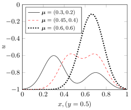
Figure 2: Parameterized obstacle $g(\bm{\gamma})$.

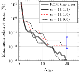
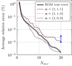
Figure 3: Convergence of Algorithm 2 for the model, parametric, static contact problem of the obstacle type: error bars shown in blue correspond to the ROMs constructed by randomly sampling the parameter space and setting $p=p_{\lambda}=20$.

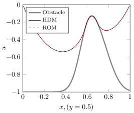
(a) $\bm{\gamma}=(0.6,0.6)$

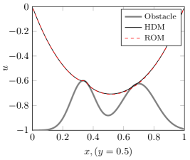
(b) $\bm{\gamma}=(0.330,0.377)$ (Maximum ROM error)

Figure 4: HDM and ROM solutions of the model, parametric, static contact problem of the obstacle type (cut view).

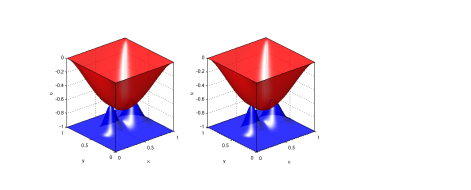
(a) HDM

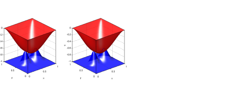
(b) ROM

Figure 5: HDM and ROM solutions for $\bm{\gamma}=(0.330,0.377)$ of the model, parametric, static contact problem of the obstacle type (full view). The obstacle and membrane are represented by the blue and red surfaces, respectively.

5.2 Dynamic contact problem of the obstacle type

Next, a dynamic version of the otherwise same model contact problem described in Section 5.1 is considered here. It is described by the inequality-constrained initial boundary value problem

$$\begin{split}\frac{\partial^{2}u}{\partial t^{2}}&=\nabla^{2}u+f\\ u&\geq g(\bm{\gamma})\\ u(x,y:0)&=0\\ \displaystyle{\frac{\partial u}{\partial t}}(x,y:0)&=0\end{split}$$ (20)

where $t\in[0,2]$.

The same semi-discrete HDM described in Section 5.1 is adopted for this problem. It is discretized in time using the implicit second-order Backward Differentiation Formula (BDF) scheme and the constant time-step $\Delta t=0.005$. The parameter domain $\mathcal{D}=(\gamma_{1},\gamma_{2})$ is set again to $[0.3,0.6]\times[0.2,0.6]$ and initially sampled on the same $10\times 10$ uniform tensor grid as before, in order to generate a set of $N_{c}=100$ candidate parameter instances. These are inputted to Algorithm 2 for performing the training procedure. At each $N_{iter}$-th iteration of Algorithm 2, the solution snapshots are collected at each time-step. Thus, the number of columns of each of the global primal and dual snapshot matrices grows in this case as $(2/0.005)\times N_{iter}=400N_{iter}$. The data compression strategy is chosen so that the size of each of the primal and dual ROBs grows as $\displaystyle{p=p_{\lambda}=\lfloor 2+(N_{iter}-1)\frac{98}{9}\rfloor}$.

Figure 6 reports on the convergence of Algorithm 2 for this problem. It reveals that in this case, all considered strategies for $\bm{\alpha}=\{\alpha_{1},\alpha_{2},\alpha_{3}\}$ perform equally well. After 10 iterations, each of these strategies leads to a ROM whose maximum amplitude error is more than 100 times smaller than that of its counterpart computed at the first iteration.

Figure 7 and Figure 8 display the time-histories at three different points in space of the solutions of problem (20) computed for two different instances of $g(\bm{\gamma})$ using in each case: (a) the HDM, (b) the ROM obtained after $10$ iterations of Algorithm 2, and (c) a variant of this ROM where SVD is used instead of NNMF to compress the dual snapshots collected within Algorithm 2. Again, note that both parameter instances $\bm{\gamma}=(0.6,0.6)$ and $\bm{\gamma}=(0.300,0.288)$ are selected here for performance assessment because neither of them is part of the training of the constructed ROM, and because $\bm{\gamma}=(0.300,0.288)$ is determined a posteriori to be the parameter instance for which the constructed ROM has the largest error. The reader can observe that as expected, the SVD-based ROMs deliver a poor performance as they do not satisfy the positivity condition of the Lagrange multipliers. On the other hand, the NNMF-based ROMs deliver a solid performance. The solutions they deliver track well the HDM solutions. This solid performance of the proposed approach for constructing a contact ROM is confirmed in Figure 9 which focuses on the entire spatial domain.

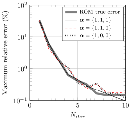
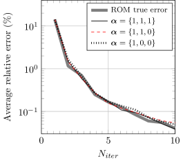
Figure 6: Convergence of Algorithm 2 for the model, parametric, dynamic contact problem of the obstacle type.

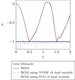
(a) $(x,y)=(0.3,0.5)$.

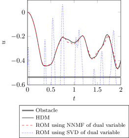
(b) $(x,y)=(0.5,0.5)$

Figure 7: Time-histories of the HDM and ROM solutions for $\bm{\gamma}=(0.6,0.6)$ of the model, parametric, dynamic contact problem of the obstacle type.

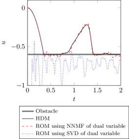
(a) $(x,y)=(0.3,0.5)$

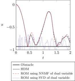
(b) $(x,y)=(0.5,0.5)$

Figure 8: Time-histories of the HDM and ROM solutions for $\bm{\gamma}=(0.300,0.288)$ of the model, parametric, dynamic contact problem of the obstacle type.

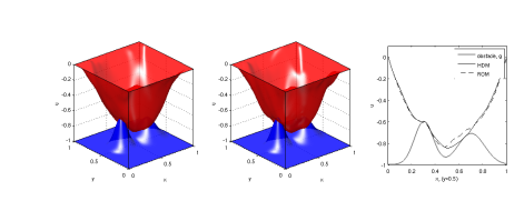
(a) HDM

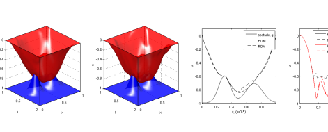
(b) ROM

Figure 9: HDM and ROM solutions at $t=0.2$, $\bm{\gamma}=(0.300,0.288)$, of the model, parametric, dynamic contact problem of the obstacle type (full view). The obstacle and membrane are represented by the blue and red surfaces, respectively.

5.3 Two-body dynamic contact problem

Finally, the two-body dynamic contact problem graphically depicted in Figure 10 is considered here.

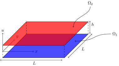
Figure 10: Two-body dynamic contact problem.

Each of the two bodies, $\Omega_{1}$ and $\Omega_{2}$, is a homogeneous, isotropic square plate of edge size $L=$1\text{\,}\mathrm{m}$$ and thickness $h=$1\text{\,}\mathrm{mm}$$. It is modeled as a linearly elastic Kirchhoff-Love plate, and therefore governed by the partial differential equation

$$\rho h\frac{\partial^{2}u}{\partial t^{2}}+D\nabla^{2}\nabla^{2}u-f=0$$ (21)

where $\rho$ denotes the density, $u(x,y:t)$ denotes the transverse displacement field, $f(x,y:t)$ denotes a distributed external force per unit area (pressure),

$$D=\frac{Eh^{3}}{12(1-\nu^{2})}$$ (22)

and $E$ and $\nu$ denote Young’s modulus and Poisson’s ratio, respectively. The two plates are assumed to be made of the same material characterized by $\rho=$7800\text{\,}\mathrm{k}\mathrm{g}\mathrm{/}\mathrm{m}^{3}$$, $E=$200\text{\,}\mathrm{G}\mathrm{P}\mathrm{a}$$, and $\nu=0.3$. One plate is positioned at $h=$4\text{\,}\mathrm{c}\mathrm{m}$$ above the other and is perfectly aligned with it. Both plates are clamped and initially at rest.

The external load per unit area $f$ is applied to the lower plate $\Omega_{1}$ only, in the upward normal direction. It is defined as $f=10^{5}f_{1}(x,y)f_{2}(t)$, where

$$f_{1}(x,y)=e^{-100\left((x-0.3)^{2}+(y-0.4)^{2}\right)}$$ (23)

$$f_{2}(t)=H(t-10\Delta t)e^{-1\times 10^{4}(t-10\Delta t)^{2}}$$ (24)

and $H$ denotes the Heaviside function.

Each plate is discretized by $100\times 100$ finite elements with 1 dof per node, resulting in a semi-discrete HDM with a total of $20,000$ dofs ($10,000$ dof for each plate). This HDM is discretized in time using the implicit second-order BDF scheme and the constant time-step $\Delta t=2\times 10^{-4}$\text{\,}\mathrm{s}$$.

For this problem, $p$ and $p_{\lambda}$ are set to $p=p_{\lambda}=40$ and Algorithm 2 is applied with $N_{c}=1$ (no parametric training) to construct a ROM of size 40. Then, this ROM is applied to the solution for $t\in[0,0.4$\text{\,}~{}${s}]$ of the same two-body dynamic contact problem as that solved using the HDM. Note that for $\Delta t=2\times 10^{-4}$\text{\,}\mathrm{s}$$, the time-interval $[0,0.4$\text{\,}\mathrm{s}$]$ is sampled in 2,000 time-steps.

Figure 11 displays the time-histories of the HDM and ROM solutions of this problem at $(x,y)=(0.5,0.5)$. It shows that the solution delivered by the constructed ROM tracks remarkably well that computed using the HDM.

Figure 12 complements Figure 11 by focusing on the computed HDM and ROM solutions at a single time-instance, $t=0.4$\text{\,}\mathrm{s}$$, but the entire computational domain. It confirms the excellent accuracy of the constructed ROM.

To illustrate the effect on the performance of a ROM of a down-sampling in time of the underlying HDM, Algorithm 2 is applied again to the construction of a series of contact ROMs in which the percentage of computed solution snapshots that are collected is uniformly decreased. To this effect, Figure 13 reports the variation of the relative error of the ROM solution with the percentage of computed solution snapshots that are collected. The reader can observe that overall, the relative error of the ROM solution is insensitive to a down-sampling in time, as long as more than 10% of the computed solution snapshots are collected for data compression. Beyond this limit, the relative error of the ROM solution increases sharply to reach the level of $52.8\%$ when only $25$ equally spaced computed solution snapshots are collected.

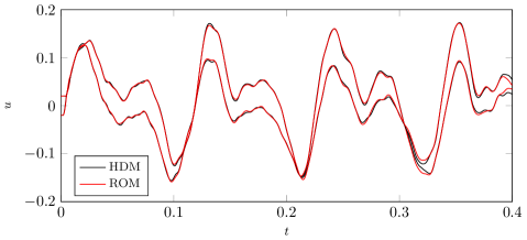
Figure 11: Time-histories of the HDM and ROM solutions of the two-body dynamic contact problem at $(x,y)=(0.5,0.5)$.

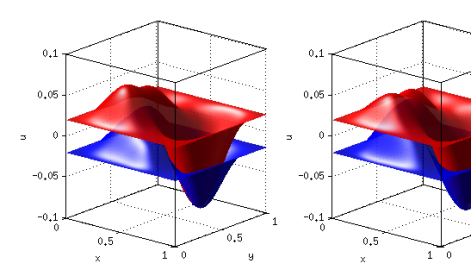
(a) HDM

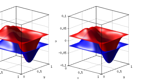
(b) $p,k=40$ ROM

Figure 12: Snapshots of HDM and ROM solutions of the two-body dynamic contact problem at $t=0.4$.

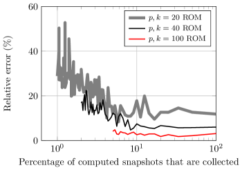
Figure 13: Effect on ROM performance of a down-sampling in time of the primal snapshots.

5.4 Computational speed-up

All model contact problems discussed above were solved in MATLAB using the quadratic program solver quadprog. Sparsity was accounted for in all algebraic entities of all HDMs. In particular, the interior-point-convex algorithm was used to solve all systems of equations arising from all HDMs. On the other hand, all small-scale and dense systems of equations arising from all ROMs were solved using the active-set algorithm. Numerical experiments revealed that among all algorithms available in quadprog, the aforementioned solvers are those which offer the best performance for the considered problems.

All CPU times were measured using the tic-toc function on a single computational thread via the -singleCompThread start-up option. For each considered contact problem, the speed-up factor delivered by its ROM for the online computations is reported in Table 1.

Table 1: Speed-ups for online computations.

Contact problem	HDM size	ROM size	Speed-up
Static, obstacle type	40,000	$p=p_{\lambda}=20$	865
Dynamic, obstacle type	40,000	$p=p_{\lambda}=100$	302
Dynamic, two-body	20,000	$p=p_{\lambda}=40$	2,229

6 Conclusions

The context of this paper is set to that of the model reduction of contact problems where the contact conditions are enforced using Lagrange multiplier degrees of freedom (dofs). In this context, constructing two separate Reduced-Order Bases (ROBs), one for the primal displacement dofs and one for the dual Lagrange multiplier dofs, is motivated and justified by the positivity condition that only the dual variables must satisfy. To this effect, it is shown in this paper that using the singular value decomposition method and the non-negative matrix factorization method to compress displacement and Lagrange multiplier snapshots, respectively, leads to effective primal and dual ROBs and a promising Galerkin projection method for the reduction of high-dimensional contact models. For parametric contact problems, it is also shown that the iterative greedy approach for sampling the parameter domain during the training of the Reduced-Order Model (ROM) can be equipped with an error indicator of reasonable offline computational complexity. This error indicator is based on the residual associated with the non-penetration condition. The computational complexity of the resulting iterative sampling and ROB construction procedure is dominated by the cost of a number of high-dimensional simulations equal to the number of sampling iterations. Specifically, for two parameterized, static and dynamic, model contact problems with 40,000 dofs, and one non-parametric two-body dynamic contact problem with 20,000 dofs, it is shown that the model reduction approach proposed in this paper and outlined above delivers online computational speedups in the range of 300 to 2,200. These are promising results which warrant the extension of the proposed model reduction approach to more realistic contact problems.

References

- [1] Moore B. Principal component analysis in linear systems: controllability, observability, and model reduction. IEEE Transactions on Automatic Control 1981; 26(1):17–32.
- [2] Grimme EJ. Krylov projection methods for model reduction. Ph.D. Thesis, University of Illinois at Urbana Champaign 1997.
- [3] Willcox K, Peraire J. Balanced model reduction via the proper orthogonal decomposition. AIAA Journal 2002; 40(11):2323–2330.
- [4] Amsallem D, Farhat C. An online method for interpolating linear parametric reduced-order models. SIAM Journal on Scientific Computing 2011; 33(5):2169–2198.
- [5] Rewienski M, White J. Model order reduction for nonlinear dynamical systems based on trajectory piecewise-linear approximations. Linear Algebra and its Applications 2006; 415(2-3):426–454.
- [6] Gu C, Roychowdhury J. Model reduction via projection onto nonlinear manifolds, with applications to analog circuits and biochemical systems. Proceedings of the 2008 IEEE/ACM International Conference on Computer-Aided Design, 2008; 85–92.
- [7] Barbič J, James DL. Real-time subspace integration for St. Venant-Kirchhoff deformable models. ACM Transactions on Graphics 2005; 24:982–990.
- [8] Balajewicz M, Dowell EH, Noack BR. Low-dimensional modelling of high-Reynolds-number shear flows incorporating constraints from the Navier–Stokes equation. Journal of Fluid Mechanics 2013; 729:285–308.
- [9] Ryckelynck D. A priori hyperreduction method: an adaptive approach. Journal of Computational Physics 2005; 202(1):346–366.
- [10] An SS, Kim T, James DL. Optimizing cubature for efficient integration of subspace deformations. ACM Transactions on Graphics (TOG) 2008; 27(5):1–10.
- [11] Chaturantabut S, Sorensen D. Nonlinear model reduction via discrete empirical interpolation. SIAM Journal on Scientific Computing 2010; 32(5):2737–2764.
- [12] Carlberg K, Bou-Mosleh C, Farhat C. Efficient non-linear model reduction via a least-squares Petrov–Galerkin projection and compressive tensor approximations. International Journal for Numerical Methods in Engineering 2011; 86(2):155–181.
- [13] Amsallem D, Zahr MJ, Farhat C. Nonlinear model order reduction based on local reduced-order bases. International Journal for Numerical Methods in Engineering 2012; 92(10):891–916.
- [14] Farhat C, Avery P, Chapman T, Cortial J. Dimensional reduction of nonlinear finite element dynamic models with finite rotations and energy‐based mesh sampling and weighting for computational efficiency. International Journal for Numerical Methods in Engineering 2014; 98(9):625–662.
- [15] Amsallem D, Zahr MJ, Choi Y, Farhat C. Design optimization using hyper-reduced-order models. Structural and Multidisciplinary Optimization 2013; :1–22.
- [16] Farhat C, Chapman T, Avery P. Structure-preserving, stability, and accuracy properties of the energy-conserving sampling and weighting method for the hyper reduction of nonlinear finite element dynamic models. International Journal for Numerical Methods in Engineering 2015; 102(5):1077–1110.
- [17] Simo JC, Laursen TA. An augmented Lagrangian treatment of contact problems involving friction. Computers & Structures 1992; 42(1):97–116.
- [18] Wriggers P. Computational Contact Mechanics. Springer, 2006.
- [19] Sirovich L. Turbulence and the dynamics of coherent structures. Part I: coherent structures. Quarterly of Applied Mathematics 1987; 45(3):561–571.
- [20] Lee DD, Seung HS. Learning the parts of objects by non-negative matrix factorization. Nature 1999; 401(6755):788–791.
- [21] Haasdonk B, Salomon J, Wohlmuth B. A reduced basis method for the simulation of American options. Numerical Mathematics and Advanced Applications. Springer Berlin Heidelberg: Berlin, Heidelberg, 2013; 821–829.
- [22] Zhang Z, Bader E, Veroy K. A duality approach to error estimation for variational inequalities. arXiv.org 2014; .
- [23] Veroy K, Patera AT. Certified real-time solution of the parametrized steady incompressible Navier-Stokes equations: rigorous reduced-basis a posteriori error bounds. International Journal for Numerical Methods in Fluids 2005; 47(8-9):773–788.
- [24] Bui-Thanh T, Willcox K, Ghattas O. Parametric reduced-order models for probabilistic analysis of unsteady aerodynamic applications. AIAA Journal 2008; 46(10):2520–2529.
- [25] Paul-Dubois-Taine A, Amsallem D. An adaptive and efficient greedy procedure for the optimal training of parametric reduced-order models. International Journal for Numerical Methods in Engineering 2015; 102(5):1262–1292.
- [26] Choi Y, Amsallem D, Farhat C. Gradient-based constrained optimization using a database of linear reduced-order models. Submitted for publication 2015; :1–21.
- [27] Kim H, Park H. Nonnegative matrix factorization based on alternating nonnegativity constrained least squares and active set method. SIAM Journal on Matrix Analysis and Applications 2008; 30(2):713–730.
- [28] Kim J, He Y, Park H. Algorithms for nonnegative matrix and tensor factorizations: a unified view based on block coordinate descent framework. Journal of Global Optimization 2013; 58(2):285–319.