Hedin’s Equations for Superconductors

Abstract

We generalize Hedin’s equations to a system of superconducting electrons coupled with a system of phonons. The electrons are described by an electronic Pauli Hamiltonian which includes the Coulomb interaction among electrons and an external vector and scalar potential. We derive the continuity equation in the presence of the superconducting condensate and point out how to cast vertex corrections in the form of a non-local effective interaction that can be used to describe both fluctuations of spin and superconducting phase beyond the screened Coulomb self-energy diagram.

I Introduction

Hedin’s formally exact iterative procedure to generate the one particle Green’s function for electrons that interact via the Coulomb potential (Hedin, 1965) has provided a useful basis for further approximations. Especially the famous GW approximation, as already introduced in the original paper, is very successful in the first principle analysis of physical system using Many-Body-Perturbation theory (Onida et al., 2002). Nowadays, with increasing computational power, even a fully self-consistent treatment of the screened Coulomb potential W within Hedin’s cycle for both, solids and molecules is in reach (Schöne and Eguiluz, 1998; Caruso et al., 2013).

While we thus have a firm foundation of ab-initio electronic structure perturbation theory, to calculate superconductivity (SC), the Green’s function approach boils down to the Eliashberg equations (Eliashberg, 1960; Scalapino et al., 1966; Carbotte, 1990). There, the Coulomb potential is usually reduced into the $\mu^{\star}$ pseudo-potential (Carbotte, 1990; Scalapino et al., 1966) and the phonons are computed externally, i.e. in the normal state. This is reasonable since the vibrational structure and the renormalized Coulomb potential appear to be largely independent on the SC condensation. Thus, in the usual Eliashberg approach, SC is computed starting from a converged normal state electronic band and phonon structure (Scalapino et al., 1966). On the other hand, spin-fluctuations are discussed as a pairing mechanism in the unconventional SC such as the cuprates and iron pnictides (Manske, 2004). With fluctuations we mean here self-energy corrections that describe effects beyond the screened Coulomb diagram. The paramagnon peak as the quasi-particle that corresponds to the spin-fluctuation interaction becomes entirely different in the SC phase (Inosov et al., 2010) and it therefore is essential to consider SC and the screening of electronic interactions on the same footing. The paramagnetic spin-fluctuations are included in ab-initio methods on a semi-ab-initio level so far. Essenberger et al. (Essenberger et al., ) have derived an effective interaction that is based on a self-energy contribution due to the magnetic susceptibility and the exchange-correlation kernel of time dependent density functional theory (Petersilka et al., 1996). We note, however, that the effective interaction derived in Ref. (Essenberger et al., ) is in the normal state and the self-energy that is used may suffer from double counting. The diagrams considered for the construction of the effective interaction are formally similar to approach of Berk and Schrieffer (Berk and Schrieffer, 1966). In the context of a Hubbard model, this approach has been extensivley used to describe the SC phase of the iron based superconductors (see Ref. Hirschfeld et al., 2011 for a review).

In a similar manner fluctuations of the SC order parameter (Larkin and Varlamov, 2008) in constrained geometries are not well described in present ab-initio methods. While the famous Mermin-Wagner theorem (Mermin and Wagner, 1966) forbids the ordering in 2D due to the onset of long wavelength fluctuations it is still unclear to what extend this result has implications in experiment. For example, SC has been observed in a lead surface on a silicone substrate down to the single atomic layer (Zhang et al., 2010). Similarly, taking the Coulomb interaction into account, the excitation energies of the collective states of paired electrons starts at the plasma frequency (Anderson, 1958; Nambu, 1960; Ambegaokar and Kadanoff, 1961). Since plasmons with a small excitation energy may exist in low dimensional systems, the collective excitations, i.e. SC fluctuations, may have to be taken into account self-consistently.

To present a fundamental theory to describe SC based on the basic interactions among electrons is the content of this paper. In particular, we derive Hedin’s equations for SC electrons that interact via the Coulomb potential and with a system of phonons in Sec. III. Our approach treats the electronic screening, the coupling to the phonons and SC on the same footing. In Sec. V, we point how to interpret vertex corrections as an effective interaction, without introducing double counting with respect to the screened Coulomb interaction. Our coupled equations are capable to describe fluctuation effects in principle exactly. This means in particular spin angular momentum transfer processes in a paramagnetic system as well as, in the language of Anderson (Anderson, 1958), iso-spin momentum transfer with respect to the Nambu off diagonal components, which corresponds to the Cooper-channel, of the Green’s function.

II The Hamiltonian

In this Section we define the basic Hamiltonian governing our system of electrons and phonons. Before we introduce the individual parts of the Hamiltonian in Eq. (6), we define the notation that we use in this work in the following separate paragraph.

Notation

To simplify the notation we introduce the usual thermal average $\langle...\rangle_{0}\equiv{\rm Tr}\bigl{\{}{\rm e}^{-\beta(\hat{H}-\mu\hat{N})}...\bigr{\}}/{\rm Tr}\bigl{\{}{\rm e}^{-\beta(\hat{H}-\mu\hat{N})}\bigr{\}}$ and $\langle\hat{A}\rangle_{{\rm{\scriptscriptstyle T}}}\equiv\langle{\rm T}\hat{U}(\beta,0)\hat{A}\rangle_{0}/\langle\hat{U}(\beta,0)\rangle_{0}$ with the time ordering symbol ${\rm T}$ and the time evolution operator $\hat{U}(\tau,\tau^{\prime})$.

Following the notation of Nambu (Nambu, 1960) and Anderson (Anderson, 1958), in order to describe it as a usual single particle Hamiltonian we introduce the Nambu field via

$$\mbox{$\hat{\varPsi}$}(\boldsymbol{{\it r}}) = \left(\begin{array}[]{cccc}\hat{\psi}(\boldsymbol{{\it r}}\uparrow)&\hat{\psi}(\boldsymbol{{\it r}}\downarrow)&\hat{\psi}^{\dagger}(\boldsymbol{{\it r}}\uparrow)&\hat{\psi}^{\dagger}(\boldsymbol{{\it r}}\downarrow)\end{array}\right)^{{\rm T}_{{\scriptscriptstyle{\rm ns}}}}\,.$$ (2)

We use ${\rm T}_{{\scriptscriptstyle{\rm ns}}}$ to transpose in Nambu (n) and spin space (s) and label Nambu components with $\alpha=1,-1$ and spin components with $\mu=\uparrow,\downarrow$. ${\rm Tr}_{{\rm{\scriptscriptstyle ns}}}$ means to take the trace in Nambu and spin space.

We further group variables in the notation

$$\begin{array}[]{cccccc}{\it 1}&=&\boldsymbol{{\it r}}_{1}\tau_{1}&\quad\bar{{\it 1}}&=&\alpha_{1}\mu_{1}\\ \int{\rm d}{\it 1}&=&\int{\rm d}\tau_{1}\int{\rm d}\boldsymbol{{\it r}}_{1}&\quad\sum_{\bar{{\it 1}}}&=&\sum_{\mu_{1}\alpha_{1}}\\ \updelta_{1,2}&=&\updelta(\boldsymbol{{\it r}}_{1}-\boldsymbol{{\it r}}_{2})\times&\quad\updelta_{\bar{{\it 1}},\bar{{\it 2}}}&=&\updelta_{\alpha_{1}\alpha_{2}}\updelta_{\mu_{1}\mu_{2}}\\ &&\times\updelta(\tau_{1}-\tau_{2})\end{array}$$ (3)

The bar indicates Nambu-spin. Thus, similarly, we indicate matrices in Nambu and spin space with a bar on top. For example, in this notation, the electronic single particle Green’s function reads

$$\bar{G}(\boldsymbol{{\it r}}\tau,\boldsymbol{{\it r}}^{\prime}\tau^{\prime}) = -\langle\hat{\varPsi}_{{\rm I}}(\boldsymbol{{\it r}}\tau)\otimes\hat{\varPsi}_{{\rm I}}^{\dagger}(\boldsymbol{{\it r}}^{\prime}\tau^{\prime})\rangle_{{\rm{\scriptscriptstyle T}}}\,.$$ (4)

The symbol $\otimes$ means to take the outer product in Nambu and spin space and the subscript ${\rm I}$ refers to an operator in the Heisenberg picture $\hat{O}_{{\rm I}}(\tau)=\hat{U}(0,\tau)\hat{O}\hat{U}(\tau,0)$. We promote the Nambu and spin indices to the argument to refer to the matrix elements, similar to the usual matrix notation. There, for a matrix $A$, one refers to the matrix elements as $A_{ij}$. $\bar{G}({\it 1}\bar{{\it 1}},{\it 2}\bar{{\it 2}})$ is thus the $\alpha_{1}\sigma_{1},\alpha_{2}\sigma_{2}$ matrix element in Nambu and spin space - a function of two space and time variables ${\it 1}$ and ${\it 2}$, respectively. We use this matrix element notation also for higher order tensors, such as $I({\it 1}\bar{{\it 1}},{\it 2}\bar{{\it 2}},{\it 3}\bar{{\it 3}},{\it 4}\bar{{\it 4}})$ which is the $(\alpha_{1}\sigma_{1},\alpha_{2}\sigma_{2},\alpha_{3}\sigma_{3},\alpha_{4}\sigma_{4})$ component of the $4\times 4\times 4\times 4$ object $I({\it 1},{\it 2},{\it 3},{\it 4})$.

If indexes appear on one side of an equation and not on the other we define that these are summed or integrated.

We use the Pauli matrices both in spin as well as in Nambu space. For the spin-Pauli matrices we use $\sigma_{0,x,y,z}$ while for the latter we use $\tau_{0,x,y,z}$.

We introduce the Nambu time ordering symbol

$$\bar{{\rm T}}\hat{\varPsi}_{{\rm I}}(\boldsymbol{{\it r}}\tau)\otimes\hat{\varPsi}_{{\rm I}}^{\dagger}(\boldsymbol{{\it r}}^{\prime}\tau^{\prime}) = \theta(\tau-\tau^{\prime})\hat{\varPsi}_{{\rm I}}(\boldsymbol{{\it r}}\tau)\otimes\hat{\varPsi}_{{\rm I}}^{\dagger}(\boldsymbol{{\it r}}^{\prime}\tau^{\prime})$$

$$- \theta(\tau^{\prime}-\tau)\bigl{(}\hat{\varPsi}_{{\rm I}}^{\dagger}(\boldsymbol{{\it r}}^{\prime}\tau^{\prime})\otimes\hat{\varPsi}_{{\rm I}}(\boldsymbol{{\it r}}\tau)\bigr{)}^{{\rm T}_{\text{sn}}}$$

This form is equivalent to a time ordering in every component of the Nambu and spin matrix. Note a peculiarity in the equal time limit: We define that the $\alpha,\alpha^{\prime}=-1,-1$ component behaves different to the $1,1$ component in the sense that here the second argument is taken infinitesimally after the first. The reason is that in the equal time limit it is necessary to recover the density operator $\hat{n}(\boldsymbol{{\it r}})=\hat{\psi}^{\dagger}(\boldsymbol{{\it r}})\cdot\sigma_{0}\cdot\hat{\psi}(\boldsymbol{{\it r}})$, also in the Nambu $-1,-1$ channel. This equal time limit appears in the interactions in a diagrammatic expansion so the definition must be chosen to recover this limit (Fetter and Walecka, 1971). The missing reordering of the operators causes an additional minus sign and thus $\hat{n}_{{\rm I}}(\boldsymbol{{\it r}}\tau)\equiv-(1/2){\rm Tr}_{{\rm{\scriptscriptstyle ns}}}\{\lim_{\tau^{\prime}\rightarrow\tau}\tau_{z}\cdot\bar{{\rm T}}\hat{\varPsi}_{{\rm I}}(\boldsymbol{{\it r}}\tau)\otimes\hat{\varPsi}_{{\rm I}}^{\dagger}(\boldsymbol{{\it r}}\tau^{\prime})\}$ with $\tau_{z}$ instead of $\tau_{0}$ without the reordering.

Contributions to the Hamiltonian

Our starting point is a system of interacting electrons that is coupled with a system of non-interacting phonons

$$\hat{H} = \hat{H}_{{\scriptscriptstyle{\rm 0}}}+\hat{H}_{{\scriptscriptstyle{\rm p}}}+\hat{H}_{{\scriptscriptstyle{\rm e}-{\rm e}}}+\hat{H}_{{\scriptscriptstyle{\rm e}-{\rm p}}}+\hat{H}_{{\scriptscriptstyle{\rm aux}}}\,.$$ (6)

Here we distinguish the single particle part $\hat{H}_{{\scriptscriptstyle{\rm 0}}}$, the non-interacting phonon part $\hat{H}_{{\scriptscriptstyle{\rm p}}}$, the electron-electron interaction $\hat{H}_{{\scriptscriptstyle{\rm e}-{\rm e}}}$, the electron-phonon interaction $\hat{H}_{{\scriptscriptstyle{\rm e}-{\rm p}}}$ and an auxiliary external potential that is set to zero after the derivation. In the single particle part $\hat{H}_{{\scriptscriptstyle{\rm 0}}}$ we distinguish $\hat{H}_{{\scriptscriptstyle{\rm 0}}}=\hat{H}_{{\scriptscriptstyle{\rm n}}}+\hat{H}_{{\scriptscriptstyle{\rm s}}}$ with a normal state $\hat{H}_{{\scriptscriptstyle{\rm n}}}$ and SC part $\hat{H}_{{\scriptscriptstyle{\rm s}}}$. The normal state part is $\hat{H}_{{\scriptscriptstyle{\rm n}}}=\int{\rm d}\boldsymbol{{\it r}}\hat{\psi}^{\dagger}(\boldsymbol{{\it r}})\cdot\hat{H}_{{\scriptscriptstyle{\rm n}}}(\boldsymbol{{\it r}})\cdot\hat{\psi}(\boldsymbol{{\it r}})$ and $\hat{\psi}(\boldsymbol{{\it r}}\mu)$ is the electron spin $\mu$ field operator. Then, the normal state contribution of the single particle part of the Hamiltonian reads

$$\hat{H}_{{\scriptscriptstyle{\rm n}}}(\boldsymbol{{\it r}}) = \sigma_{0}\Bigl{(}\frac{1}{2}\bigl{(}-{\rm i}\boldsymbol{\nabla}+\boldsymbol{A}_{{\scriptscriptstyle{\rm ext}}}(\boldsymbol{{\it r}})\bigr{)}^{2}+\phi_{{\scriptscriptstyle{\rm ext}}}(\boldsymbol{{\it r}})\Bigr{)}+$$ (7)

$$+ \mathbf{S}\cdot\boldsymbol{B}_{{\scriptscriptstyle{\rm ext}}}(\boldsymbol{{\it r}})\,.$$

Here $\boldsymbol{B}_{{\scriptscriptstyle{\rm ext}}}(\boldsymbol{{\it r}})=\boldsymbol{\nabla}\times\boldsymbol{A}_{{\scriptscriptstyle{\rm ext}}}(\boldsymbol{{\it r}})$, $\mathbf{S}=(\begin{array}[]{ccc}\sigma_{x}&\sigma_{y}&\sigma_{z}\end{array})^{{\rm T}}$ and $\boldsymbol{A}_{{\scriptscriptstyle{\rm ext}}}(\boldsymbol{{\it r}})$ is an external vector potential. Further $\phi_{{\scriptscriptstyle{\rm ext}}}(\boldsymbol{{\it r}})$ is the scalar potential including the Coulomb attraction of the ions in their equilibrium position. The existence of a pair condensate with a macroscopic number of electron pairs is measured with the order parameter of SC $\boldsymbol{\chi}(\boldsymbol{{\it r}},\boldsymbol{{\it r}}^{\prime})=\langle\hat{\psi}(\boldsymbol{{\it r}})\cdot\boldsymbol{\Phi}\cdot\hat{\psi}(\boldsymbol{{\it r}}^{\prime})\rangle$ where $\hat{\psi}(\boldsymbol{{\it r}})=\bigl{(}\begin{array}[]{cc}\hat{\psi}(\boldsymbol{{\it r}}\uparrow)&\hat{\psi}(\boldsymbol{{\it r}}\downarrow)\end{array}\bigr{)}^{{\rm T}}$. The 4 component vector $\boldsymbol{\Phi}=(\begin{array}[]{cccc}{\rm i}\sigma_{y}&-\sigma_{z}&\sigma_{0}&\sigma_{x}\end{array})^{{\rm T}}$ parametrizes the order parameter into 1 singlet $\Phi_{1}$ and 3 triplet parts $\Phi_{2},\Phi_{3},\Phi_{4}$. The singlet and triplet SC part of the total Hamiltonian that couples to an external singlet and triplet pairing field $\boldsymbol{\varDelta}_{{\scriptscriptstyle{\rm ext}}}^{\ast}(\boldsymbol{{\it r}},\boldsymbol{{\it r}}^{\prime})$ is

$$\hat{H}_{{\scriptscriptstyle{\rm s}}} = -\frac{1}{2}\int{\rm d}\boldsymbol{{\it r}}\int{\rm d}\boldsymbol{{\it r}}^{\prime}\bigl{(}\hat{\psi}(\boldsymbol{{\it r}})\cdot\boldsymbol{\Phi}\cdot\hat{\psi}(\boldsymbol{{\it r}}^{\prime})\cdot\boldsymbol{\varDelta}_{{\scriptscriptstyle{\rm ext}}}^{\ast}(\boldsymbol{{\it r}},\boldsymbol{{\it r}}^{\prime})$$ (8)

$$- \hat{\psi}^{\dagger}(\boldsymbol{{\it r}})\cdot\boldsymbol{\Phi}\cdot\hat{\psi}^{\dagger}(\boldsymbol{{\it r}}^{\prime})\cdot\boldsymbol{\varDelta}_{{\scriptscriptstyle{\rm ext}}}(\boldsymbol{{\it r}},\boldsymbol{{\it r}}^{\prime})\bigr{)}\,.$$

Here, the combination $\boldsymbol{\varDelta}_{{\scriptscriptstyle{\rm ext}}}(\boldsymbol{{\it r}},\boldsymbol{{\it r}}^{\prime})\cdot\boldsymbol{\Phi}_{\mu\mu^{\prime}}=-\boldsymbol{\varDelta}_{{\scriptscriptstyle{\rm ext}}}(\boldsymbol{{\it r}}^{\prime},\boldsymbol{{\it r}})\cdot\boldsymbol{\Phi}_{\mu^{\prime}\mu}$ is totally antisymmetric. Thus, the pair Hamiltonian Eq. 8 is hermitian by construction. We use $q=\boldsymbol{{\it q}},\lambda$ with the Bloch vector $\boldsymbol{{\it q}}$ and the mode number $\lambda$ to indicate the quantum number on the phonon operators $\hat{b}_{q}$. Then, the phononic single particle Hamiltonian is

$$\hat{H}_{{\scriptscriptstyle p}} = \sum_{q}\varOmega_{q}(\hat{b}_{q}^{\dagger}\hat{b}_{q}+\frac{1}{2})\,.$$ (9)

We assume the electrons to interact via a spontaneous Coulomb interaction

$$\hat{H}_{{\scriptscriptstyle{\rm e}-{\rm e}}} = \frac{1}{2}\sum_{\mu\mu^{\prime}}\!\int{\rm d}\boldsymbol{{\it r}}\int{\rm d}\boldsymbol{{\it r}}^{\prime}w_{{\scriptscriptstyle{\rm 0}}}(\boldsymbol{{\it r}},\boldsymbol{{\it r}}^{\prime})\times$$ (10)

$$\times \hat{\psi}^{\dagger}\!(\boldsymbol{{\it r}}\mu)\hat{\psi}^{\dagger}\!(\boldsymbol{{\it r}}^{\prime}\mu^{\prime})\hat{\psi}(\boldsymbol{{\it r}}^{\prime}\mu^{\prime})\hat{\psi}(\boldsymbol{{\it r}}\mu)\,,$$ (11)

with $w_{{\scriptscriptstyle{\rm 0}}}(\boldsymbol{{\it r}},\boldsymbol{{\it r}}^{\prime})=1/|\boldsymbol{{\it r}}-\boldsymbol{{\it r}}^{\prime}|$. $w_{{\scriptscriptstyle{\rm 0}}}(\boldsymbol{{\it r}},\boldsymbol{{\it r}}^{\prime})$ is independent of spin and also the screened potential will share this property. Following Ref. (Aryasetiawan and Biermann, 2008) one could start with a spin dependent interaction. In this work we take a different route. After the derivation of Hedin’s equations for a SC, we discuss the important self-energy diagrams that form an effective spin dependent interaction.and the electron phonon interaction is (we use the notation $-q\equiv-\boldsymbol{{\it q}},\lambda$ and $i=0,x,y,z$)

$$\hat{H}_{{\scriptscriptstyle{\rm e}-{\rm p}}} = \sum_{iq}\int{\rm d}\boldsymbol{{\it r}}\hat{\psi}^{\dagger}(\boldsymbol{{\it r}})\cdot\sigma_{i}\cdot\hat{\psi}(\boldsymbol{{\it r}})g_{i}(\boldsymbol{{\it r}}q)(\hat{b}_{q}+\hat{b}_{-q}^{\dagger})\,.$$ (12)

Because $\hat{H}_{{\scriptscriptstyle{\rm e}-{\rm p}}}$ is hermitian, $g_{i}(\boldsymbol{{\it r}}q)$ satisfies $g_{i}(\boldsymbol{{\it r}}q)=g_{i}^{\ast}(\boldsymbol{{\it r}},-q)$. The operator $\hat{H}_{{\scriptscriptstyle{\rm s}}}$ is not diagonal in the electronic field operator $\hat{\psi}(\boldsymbol{{\it r}})$. To derive the Hedin equations we use the auxiliary external fields $\varphi(\boldsymbol{r}\tau)$ and $J_{q}(\tau)$ that are set to zero after the derivation. We define

$$\hat{H}_{{\scriptscriptstyle{\rm aux}}} = \hat{H}_{{\scriptscriptstyle{\rm aux}}}^{0}+\hat{H}_{{\scriptscriptstyle{\rm aux}}}^{p}\,,$$ (13)

and choose $\hat{H}_{{\scriptscriptstyle{\rm aux}}}^{0}(\tau_{1})=\int{\rm d}\boldsymbol{r}_{1}\varphi({\it 1})\hat{\psi}^{\dagger}(\boldsymbol{{\it r}}_{1})\cdot\sigma_{0}\cdot\hat{\psi}(\boldsymbol{{\it r}}_{1})$ and $\hat{H}_{{\scriptscriptstyle{\rm aux}}}^{p}=J_{q}(\hat{b}_{q}+\hat{b}_{-q}^{\dagger})$ where $J_{-q}=J_{q}^{\ast}$ to make the operator hermitian.

III Hedin’s Equations for Superconductors

In this Section, we derive the Hedin equations for a superconductor. We point out that we can work in the ground state, the equilibrium finite temperature (Fetter and Walecka, 1971) or the more general Keldysh formalism (Stefanucci and van Leeuwen, 2013). The Hedin equation formally have the same shape. Here we work in the equilibrium finite temperature formalism for definiteness. Our starting point is the equation of motion of the single particle Green’s function. We express the two particle part as a functional derivative with respect to the auxiliary field. Using a similar strategy for the appearing self-energy and vertex terms leads to a set of closed equations, independent on the auxiliary potential - the Hedin equations.

III.1 Green’s Function Dyson Equation

In the following we derive the Dyson equation for the electronic Green’s function from the equation of motion

$$-\partial_{\tau_{1}}\bar{G}({\it 1}\bar{{\it 1}},{\it 2}\bar{{\it 2}}) = \updelta_{{\it 1},{\it 2}}\updelta_{\bar{{\it 1}},\bar{{\it 2}}}+$$ (14)

$$+ \langle[\hat{H},\hat{\varPsi}(\boldsymbol{{\it r}}_{1}\bar{{\it 1}})]_{{\rm I}}(\tau_{1})\hat{\varPsi}_{{\rm I}}^{\dagger}({\it 2}\bar{{\it 2}})\rangle_{{\rm{\scriptscriptstyle T}}}\,.$$

Similarly to the original derivation, we are describing the two particle part of the equation of motion as the functional derivative with respect to the auxiliary field $\varphi({\it 1})$. Note here that although $\hat{H}$ and $\updelta\hat{H}/\updelta\varphi(1)$ do not commute in the case of a SC, the time ordering still allows us to use $\frac{\updelta}{\updelta\varphi(1)}\bar{{\rm T}}\hat{U}(\beta,0)=\frac{1}{2}\bar{{\rm T}}\hat{U}(\beta,0)\hat{\varPsi}_{{\rm I}}^{\dagger}({\it 1})\cdot\sigma_{0}\tau_{z}\cdot\hat{\varPsi}_{{\rm I}}({\it 1})$. We complete the derivation of the Dyson equation in the Appendix A with the result

$$\bar{G}({\it 1},{\it 2}) = \bar{G}_{{\rm{\scriptscriptstyle H}}}({\it 1},{\it 2})+\bar{G}_{{\rm{\scriptscriptstyle H}}}({\it 1},{\it 3})\cdot\bar{\varSigma}({\it 3},{\it 4})\cdot\bar{G}({\it 4},{\it 2})\,.$$

Also the self-energy $\bar{\varSigma}({\it 3},{\it 4})$ is defined in the Appendix A. Our Dyson equation starts from the Hartree Green’s function $\bar{G}_{{\rm{\scriptscriptstyle H}}}({\it{\it 3}},{\it 2})$ that satisfies

$$\bigl{(}-\tau_{0}\sigma_{0}\partial_{\tau_{1}}\delta_{{\it 1},{\it 3}}-\hat{\bar{H}}_{{\rm{\scriptscriptstyle H}}}({\it 1},{\it 3})\bigr{)}\cdot\bar{G}_{{\rm{\scriptscriptstyle H}}}({\it{\it 3}},{\it 2}) = \updelta_{{\it 1},{\it 2}}\sigma_{0}\tau_{0}$$

where the Nambu and spin matrix operator $\hat{\bar{H}}_{{\rm{\scriptscriptstyle H}}}({\it 1},{\it 3})$ in first quantization is given by $\hat{\bar{H}}_{{\rm{\scriptscriptstyle H}}}({\it 1},{\it 3})=\hat{\bar{H}}_{{\scriptscriptstyle 0}}({\it 1},{\it 3})+\varPhi({\it 1})\sigma_{0}\tau_{z}\delta_{{\it 1},{\it 3}}$ with the Hartree field $\varPhi({\it 1})=\int n(\boldsymbol{{\it r}})w_{{\scriptscriptstyle{\rm 0}}}(\boldsymbol{{\it r}}_{1},\boldsymbol{{\it r}}){\rm d}\boldsymbol{{\it r}}+\varphi({\it 1})$ where $n(\boldsymbol{r})$ is the electron density. The bare Hamiltonian is

$$\hat{\bar{H}}_{{\scriptscriptstyle{\rm 0}}}({\it 1},{\it 3}) = \left(\begin{array}[]{cc}\hat{H}_{{\scriptscriptstyle{\rm n}}}({\it 1})\updelta_{{\it 1,3}}&\boldsymbol{\varDelta}_{{\scriptscriptstyle{\rm ext}}}({\it 1},{\it 3})\cdot\boldsymbol{\Phi}\\ -\boldsymbol{\varDelta}_{{\scriptscriptstyle{\rm ext}}}^{\ast}({\it 1},{\it 3})\cdot\boldsymbol{\Phi}&-\bigl{(}\hat{H}_{{\scriptscriptstyle{\rm n}}}({\it 1})\bigr{)}^{{\rm T}_{{\scriptscriptstyle{\rm s}}}}\updelta_{{\it 1,3}}\end{array}\right)\,,$$ (19)

with the normal state part $\hat{H}_{{\scriptscriptstyle{\rm n}}}$ of the total Hamiltonian given in Eq. (7). Note that because of the total anti-symmetry of $\boldsymbol{\varDelta}_{{\scriptscriptstyle{\rm ext}}}({\it 1},{\it 3})\cdot\boldsymbol{\Phi}$ and $\mathbf{S}^{{\rm T}_{{\scriptscriptstyle{\rm s}}}}=\mathbf{S}^{\ast}$ the bare Hamiltonian $\hat{\bar{H}}_{{\scriptscriptstyle{\rm 0}}}$ is hermitian. The self-energy $\bar{\varSigma}({\it 3},{\it 4})$ so far remains in the form given in the Appendix A, Eq. (63) which depends on the auxiliary potentials. In the next two Subsections we give self consistent equations for the phononic and electronic part in terms of the Green’s function and the vertex, thereby removing this dependence on the auxiliary potentials.

III.2 Phonon Propagator, Vertex and Self-Energy

In this Subsection cast the functional derivative with respect to the auxiliary potentials into a dependence on the Green’s function only. As a preparatory, we introduce the bare phonon vertex

$$\bar{\varGamma}_{{\scriptscriptstyle{\rm ph}}}^{{\scriptscriptstyle{\rm 0}}}({\it 1}\bar{{\it 1}},{\it 2}\bar{{\it 2}};q\tau_{3}) = (\bar{v}_{i})_{\bar{{\it 1}}\bar{{\it 2}}}g_{i}(\boldsymbol{{\it r}}_{1}q)\updelta_{{\it 1}{\it 2}}\updelta_{\tau_{3}\tau_{1}}\,,$$ (21)

where $\bar{\boldsymbol{v}}=(\begin{array}[]{cccc}\tau_{z}\sigma_{0}&\tau_{z}\sigma_{x}&\tau_{0}\sigma_{y}&\tau_{z}\sigma_{z}\end{array})$ and we use the abbreviation $\hat{a}_{q}=\hat{b}_{q}+\hat{b}_{-q}^{\dagger}$. The self-energy $\bar{\varSigma}$ of Eq. (63) in the Appendix A consists of the parts $\bar{\varSigma}({\it 1},{\it 2})=\bar{\varSigma}_{{\scriptscriptstyle{\rm xc}}}({\it 1},{\it 2})+\bar{\varSigma}_{{\scriptscriptstyle{\rm ph}}}^{{\scriptscriptstyle{\rm H}}}({\it 1},{\it 2})$. Here, $\bar{\varSigma}_{{\scriptscriptstyle{\rm xc}}}({\it 1},{\it 2})=\bar{\varSigma}_{{\scriptscriptstyle{\rm C}}}({\it 1},{\it 2})+\bar{\varSigma}_{{\scriptscriptstyle{\rm ph}}}({\it 1},{\it 2})$ which separates an electronic and a phononic part. Thus, phonon self-energy contributions to $\bar{\varSigma}({\it 1},{\it 2})$ are given by

$$\bar{\varSigma}_{{\scriptscriptstyle{\rm ph}}}^{{\scriptscriptstyle{\rm H}}}({\it 1},{\it 2}) = \bar{\varGamma}_{{\scriptscriptstyle{\rm ph}}}^{{\scriptscriptstyle{\rm 0}}}({\it 1},{\it 2};q\tau_{3})\langle\hat{a}_{q}(\tau_{3})\rangle_{{\rm{\scriptscriptstyle T}}}$$ (22)

$$\bar{\varSigma}_{{\scriptscriptstyle{\rm ph}}}({\it 1},{\it 2}) = \bar{\varGamma}_{{\scriptscriptstyle{\rm ph}}}^{{\scriptscriptstyle{\rm 0}}}({\it 1},{\it 3};q\tau_{4})\cdot\bar{G}({\it 3},{\it 4})\cdot$$ (23)

$$\cdot\bar{\varGamma}_{{\scriptscriptstyle{\rm ph}}}({\it 4},{\it 2};q^{\prime}\tau^{\prime})D_{{\scriptscriptstyle{\rm ph}}}(q\tau_{4},-q^{\prime}\tau_{5})\,.$$

The Hartree part $\bar{\varSigma}_{{\scriptscriptstyle{\rm ph}}}^{{\scriptscriptstyle{\rm H}}}({\it 1},{\it 2})$ is separated in order that we obtain a phononic vertex equation with a bare term Eq. (21), later. We have introduced the phonon propagator $D_{{\scriptscriptstyle{\rm ph}}}(q\tau,q^{\prime}\tau^{\prime})=\updelta\langle\hat{a}_{-q^{\prime}}(\tau^{\prime})\rangle_{{\rm{\scriptscriptstyle T}}}/\updelta J_{q}(\tau)$ and the phonon vertex $\bar{\varGamma}_{{\scriptscriptstyle{\rm ph}}}({\it 1},{\it 2};q\tau)=\updelta\bar{G}^{-1}({\it 1},{\it 2})/\updelta\langle\hat{a}_{q}(\tau)\rangle_{{\rm{\scriptscriptstyle T}}}$. Evaluating commutators with the Hamiltonian Eq. (6) and using $\varOmega_{q}=\varOmega_{-q}$ we obtain the equation of motion

$$T\partial_{\tau}^{2}\hat{a}_{q}(\tau) = 2\varOmega_{q}^{2}\hat{a}_{q}(\tau)$$

$$- 2\varOmega_{q}\bar{\varGamma}_{{\scriptscriptstyle{\rm ph}}}^{{\scriptscriptstyle{\rm 0}}}({\it 1}\bar{{\it 1}},{\it 2}\bar{{\it 2}};-q\tau_{3})T\hat{\varPsi}({\it 1}\bar{{\it 1}})\hat{\varPsi}^{\dagger}({\it 2}\bar{{\it 2}})\,.$$

Further using Eq. (62) it is straight forward to derive a Dyson equation for $D_{{\scriptscriptstyle{\rm ph}}}(q\tau,q^{\prime}\tau^{\prime})$

$$D_{{\scriptscriptstyle{\rm ph}}}(q\tau,q^{\prime}\tau^{\prime}) = D_{{\scriptscriptstyle{\rm ph}}}^{{\rm{\scriptscriptstyle 0}}}(q\tau,q^{\prime}\tau^{\prime})+D_{{\scriptscriptstyle{\rm ph}}}^{{\rm{\scriptscriptstyle 0}}}(q\tau,k\tau_{k})\times$$ (25)

$$\times \bar{\varGamma}_{{\scriptscriptstyle{\rm ph}}}^{{\scriptscriptstyle{\rm 0}}}({\it 1}\bar{{\it 1}},{\it 2}\bar{{\it 2}};-q\tau_{3})\bar{G}({\it 3}\bar{{\it 3}},{\it 2}\bar{{\it 2}})\times$$

$$\times \bar{G}({\it 1}\bar{{\it 1}},{\it 4}\bar{{\it 4}})\bar{\varGamma}_{{\scriptscriptstyle{\rm ph}}}({\it 4}\bar{{\it 4}},{\it 3}\bar{{\it 3}};k^{\prime}\tau_{k}^{\prime})\times$$

$$\times D_{{\scriptscriptstyle{\rm ph}}}(k^{\prime}\tau_{k}^{\prime},q^{\prime}\tau^{\prime})\,,$$

with the bare phonon propagator

$$\bigl{(}\partial_{\tau}^{2}-\varOmega_{q}^{2}\bigr{)}D_{{\scriptscriptstyle{\rm ph}}}^{{\rm{\scriptscriptstyle 0}}}(q\tau,q^{\prime}\tau^{\prime})=2\varOmega_{q}\updelta_{q,-q^{\prime}}\updelta(\tau-\tau^{\prime})\,.$$ (26)

The phonon vertex in turn satisfies

$$\bar{\varGamma}_{{\scriptscriptstyle{\rm ph}}}({\it 1},{\it 2};q^{\prime}\tau^{\prime}) = \bar{\varGamma}_{{\scriptscriptstyle{\rm ph}}}^{{\scriptscriptstyle{\rm 0}}}({\it 1},{\it 2};q\tau_{3})+\frac{\updelta\bar{\varSigma}_{{\scriptscriptstyle{\rm xc}}}({\it 1}\bar{{\it 1}},{\it 2}\bar{{\it 2}})}{\updelta\bar{G}({\it 4}\bar{{\it 4}},{\it 5}\bar{{\it 5}})}\times$$

$$\times \bar{G}({\it 4}\bar{{\it 4}},{\it 6}\bar{{\it 6}})\bar{\varGamma}_{{\scriptscriptstyle{\rm ph}}}({\it 6}\bar{{\it 6}},{\it 7}\bar{{\it 7}};q\tau_{3})\bar{G}({\it 7}\bar{{\it 7}},{\it 5}{\it\bar{5}})\,.$$

Thus all terms in the Eqs. (22) and (23) do not dependent explicitly on the auxiliary potentials.

III.3 Coulomb Vertex and Self-Energy

Repeating the above procedure for the electron-electron interaction leads to an expression for the electronic self-energy in terms of the electron vertex and the screened interaction. Using the chain rule, the electronic self-energy in Eq. (63) can be cast into

$$\bar{\varSigma}_{{\scriptscriptstyle{\rm C}}}({\it 1},{\it 2}) = w({\it 1},{\it 4})\tau_{z}\sigma_{0}\cdot\bar{G}({\it 1},{\it 3})\cdot\bar{\varGamma}_{{\scriptscriptstyle{\rm C}}}({\it 3},{\it 2};{\it 4})\,.$$ (28)

We introduce $\bar{\varGamma}_{{\scriptscriptstyle{\rm C}}}({\it 1},{\it 2};{\it 3})=-\updelta\bar{G}^{-1}({\it 1},{\it 2})/\updelta\varPhi({\it 3})$ as the electronic vertex and derive its Dyson equation with the notation $\bar{\varGamma}_{{\scriptscriptstyle{\rm C}}}^{{\scriptscriptstyle{\rm 0}}}({\it 1},{\it 2};{\it 3})=\sigma_{0}\tau_{z}\delta_{{\it 1},{\it 2}}\delta_{{\it 1},{\it 3}}$

$$\bar{\varGamma}_{{\scriptscriptstyle{\rm C}}}({\it 1},{\it 2};{\it 3}) = \bar{\varGamma}_{{\scriptscriptstyle{\rm C}}}^{{\scriptscriptstyle{\rm 0}}}({\it 1},{\it 2};{\it 3})+\frac{\updelta\bar{\varSigma}({\it 1}\bar{{\it 1}},{\it 2}\bar{{\it 2}})}{\updelta\bar{G}({\it 4}\bar{{\it 4}},{\it 5}\bar{{\it 5}})}\times$$

$$\times \bar{G}({\it 4}\bar{{\it 4}},{\it 6}\bar{{\it 6}})\bar{\varGamma}_{{\scriptscriptstyle{\rm C}}}({\it 6}\bar{{\it 6}},{\it 7}\bar{{\it 7}};{\it 3})\bar{G}({\it 7}\bar{{\it 7}},{\it 5}\bar{{\it 5}})\,.$$

At this point we have a Dyson equation for the electronic single particle Green function (Eq. (LABEL:eq:GFDysonEquation)), the phonon propagator (Eq. (25)) and the vertices (Eqs. (LABEL:eq:PhononVertex) and (LABEL:eq:CoulombVertex)) to construct the self-energy self-consistently. The self-energy $\bar{\varSigma}_{{\scriptscriptstyle{\rm C}}}$ contains, in addition, the screened interaction $w({\it 1},{\it 2})=w_{{\scriptscriptstyle{\rm 0}}}({\it 1},{\it 3})\updelta\varPhi({\it 3})/\updelta\varphi({\it 2})$. Inserting the definition of the Hartree field and using the chain rule we conclude that $w({\it 1},{\it 2})$ satisfies

$$w({\it 1},{\it 2}) = w_{{\scriptscriptstyle{\rm 0}}}({\it 1},{\it 2})+w_{{\scriptscriptstyle{\rm 0}}}({\it 1},{\it 3})P({\it 3},{\it 4})w({\it 2},{\it 4})$$ (30)

where the polarization $P({\it 1},{\it 2})=\updelta n({\it 1})/\updelta\varPhi({\it 2})$ can be cast into

$$P({\it 1},{\it 2}) = \frac{1}{2}{\rm Tr}_{{\rm{\scriptscriptstyle ns}}}\bigl{\{}\sigma_{0}\tau_{z}\cdot\bar{G}({\it 1},{\it 3})\cdot\bar{\varGamma}_{{\scriptscriptstyle{\rm C}}}({\it 3},{\it 4};{\it 2})\cdot\bar{G}({\it 4},{\it 1})\bigr{\}}\,,$$

where we have used $n({\it 1})={\rm Tr}_{{\rm{\scriptscriptstyle ns}}}\bigl{\{}\sigma_{0}\tau_{z}\cdot\bar{G}({\it 1},{\it 1})\bigr{\}}/2$ which concludes our self-consistent Hedin cycle. This collection of self-consistent equations is represented diagrammatically in Fig. 1

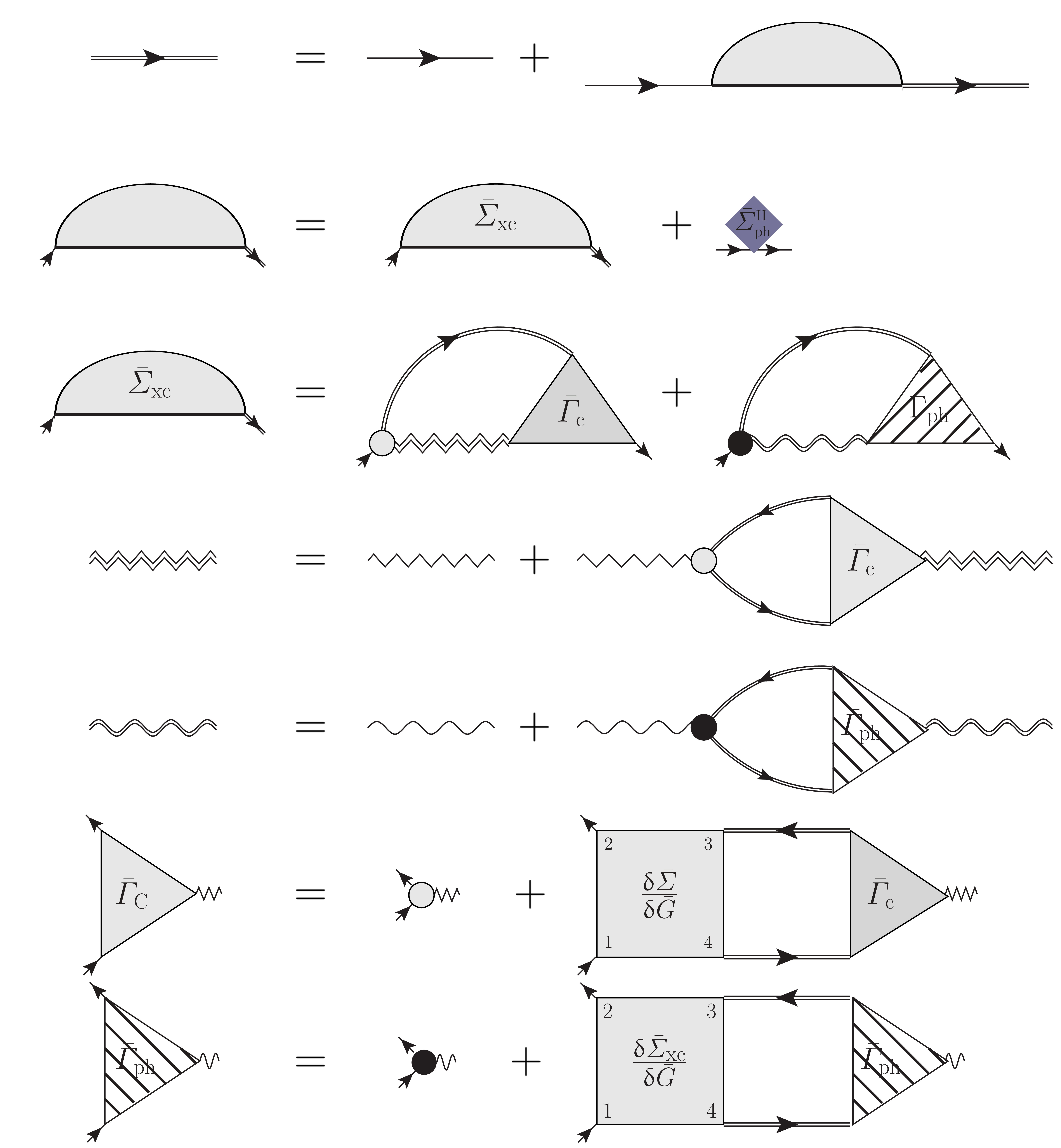
Figure 1: Diagrammatic representation of the Hedin equations for a superconductors.

. In $P({\it 1},{\it 2})$, there appear contributions from the Cooper channel that add to the screening of the bare Coulomb interaction according to Eq. 30. For example, inserting the bare Coulomb vertex $\bar{\varGamma}_{{\scriptscriptstyle{\rm C}}}^{{\scriptscriptstyle{\rm 0}}}$ for $\bar{\varGamma}_{{\scriptscriptstyle{\rm C}}}$ in Eq. LABEL:eq:PolarizationEquation the term $-\frac{1}{2}\int{\rm d}{\it 3}{\rm Tr}_{{\rm{\scriptscriptstyle s}}}\bigl{\{}\bar{G}({\it 1},-1,{\it 3},1)\bar{G}({\it 3},1,{\it 1},-1)\bigr{\}}$ with the SC Nambu off diagonal parts of the Green’s function contributes to the polarization and thus directly to the screening.

In practice, often $g_{i}(\boldsymbol{{\it r}}q)$ is taken as $\sum_{\mu\mu^{\prime}}\sigma_{i}^{\mu\mu^{\prime}}\updelta v_{{\scriptscriptstyle{\rm scf}}}(\boldsymbol{{\it r}},\mu\mu^{\prime})/\updelta u_{q}$ of a phonon calculation in density functional perturbation theory (DFPT) and similarly the phonon mode frequencies are calculated from the density response of a Kohn-Sham system in density functional theory (Baroni et al., 2001). The $\varOmega_{q}$ obtained in this way include electronic screening already and often compare well with experiment. In this case, care has to be taken not to double count electronic screening, when Eq. (25) is applied (van Leeuwen, 2004).

The question may be reformulated to what phonon system with frequencies $\varOmega_{q}$ as “bare” we should start from in order that a coupling to the electrons via Eq. (25) leads to the best dressed phonon frequencies. While for calculating SC it is often enough to neglect the influence of the electronic system on the phonon system beyond DFPT, it would be clearly interesting to investigate the influence of the SC phase on the phonon frequencies. This issue must be regarded as an open problem as of now and a further discussion is beyond the scope of this paper. In the following we shall rely on the usual approach to consider the phonons as bare $D_{{\scriptscriptstyle{\rm ph}}}\rightarrow D_{{\scriptscriptstyle{\rm ph}}}^{{\rm{\scriptscriptstyle 0}}}$ and furthermore we follow an argument of Migdal (Migdal, 1958) and Eliashberg (Eliashberg, 1960) and do not consider vertex corrections, i.e. $\bar{\varGamma}_{{\scriptscriptstyle{\rm ph}}}\rightarrow\bar{\varGamma}_{{\scriptscriptstyle{\rm ph}}}^{{\scriptscriptstyle{\rm 0}}}$.

IV The continuity equation

The external pairing field $\boldsymbol{\varDelta}_{{\scriptscriptstyle{\rm ext}}}$ and $\boldsymbol{\varDelta}_{{\scriptscriptstyle{\rm ext}}}^{\ast}$, as well as their respective self-energy renormalization on the Nambu off diagonal, act as a source and sink for electron pairs, respectively. Consequently, these terms alter the conservation laws obeyed by the exact system as compared to the normal state system. Based on the Dyson Eq. (LABEL:eq:GFDysonEquation) in the form $\bar{G}^{-1}({\it{\it 1}},{\it 2})=\bar{G}_{{\rm{\scriptscriptstyle H}}}^{-1}({\it 1},{\it 2})-\bar{\varSigma}({\it 1},{\it 2})$, we generalize the approach of Baym and Kadanoff (Baym and Kadanoff, 1961) to superconductors. In particular, we derive the continuity equation for the electronic charge. First, we realize

$$\updelta_{{\it 1},{\it 2}} = \bar{G}({\it{\it 1}},{\it 3})\cdot\bar{G}_{{\rm{\scriptscriptstyle 0}}}^{-1}({\it 3},{\it 2})$$ (32)

$$- \bar{G}({\it{\it 1}},{\it 3})\cdot\bigl{(}\bar{\varSigma}({\it 3},{\it 2})-\varPhi({\it 3})\sigma_{0}\tau_{z}\delta_{{\it 3},{\it 2}}\bigr{)}$$

$$\updelta_{{\it 1},{\it 2}} = \bar{G}_{{\rm{\scriptscriptstyle 0}}}^{-1}({\it 1},{\it 3})\cdot\bar{G}({\it{\it 3}},{\it 2})$$ (33)

$$- \bigl{(}\bar{\varSigma}({\it 1},{\it 3})-\varPhi({\it 1})\sigma_{0}\tau_{z}\delta_{{\it 1},{\it 3}}\bigr{)}\cdot\bar{G}({\it{\it 3}},{\it 2})$$

where $\bigl{(}-\tau_{0}\sigma_{0}\partial_{\tau_{1}}\updelta_{{\it 1},{\it 3}}-\hat{\bar{H}}_{{\rm{\scriptscriptstyle 0}}}({\it 1},{\it 3})\bigr{)}\bar{G}_{{\rm{\scriptscriptstyle 0}}}({\it 3},{\it 2})=\updelta_{{\it 1},{\it 2}}$ and thus

$$\bar{G}_{{\rm{\scriptscriptstyle 0}}}^{-1}({\it 1},{\it 2}) = \bigl{(}-\tau_{0}\sigma_{0}\partial_{\tau_{1}}\updelta_{{\it 1},{\it 2}}-\hat{\bar{H}}_{{\rm{\scriptscriptstyle 0}}}({\it 1},{\it 2})\bigr{)}$$ (34)

Noting that the derivative is anti-symmetric, i. e. $\partial_{\tau_{1}}\updelta_{{\it 1},{\it 2}}=-\partial_{\tau_{2}}\updelta_{{\it 1},{\it 2}}$ and $\boldsymbol{\nabla}_{\boldsymbol{r}_{1}}\updelta_{{\it 1},{\it 2}}=-\boldsymbol{\nabla}_{\boldsymbol{r}_{1}}\updelta_{{\it 1},{\it 2}}$, we calculate

$$\int{\rm d}{\it 3}\bigl{(}\bar{G}_{{\rm{\scriptscriptstyle 0}}}^{-1}({\it 1},{\it 3})\cdot\bar{G}({\it{\it 3}},{\it 2})-\bar{G}({\it{\it 1}},{\it 3})\cdot\bar{G}_{{\rm{\scriptscriptstyle 0}}}^{-1}({\it 3},{\it 2})\bigr{)}=$$ (35)

$$= \int{\rm d}{\it 3}\bigl{(}\bar{\varSigma}({\it 1},{\it 3})-\varPhi({\it 1})\sigma_{0}\tau_{z}\delta_{{\it 1},{\it 3}}\bigr{)}\cdot\bar{G}({\it{\it 3}},{\it 2})$$

$$- \bar{G}({\it{\it 1}},{\it 3})\cdot\bigl{(}\bar{\varSigma}({\it 3},{\it 2})-\varPhi({\it 3})\sigma_{0}\tau_{z}\delta_{{\it 3},{\it 2}}\bigr{)}$$

in the Appendix B. Similar to Baym and Kadanoff (Baym and Kadanoff, 1961), in addition taking into account the presence of the SC condensate many conservation laws can be deduced from this equation. We are particularly interested in the local ${\it 2}\rightarrow{\it 1}$ limit of the $1,1$ Nambu component of Eq. (65). If we take the trace in spin space, we arrive at the continuity equation for the electric charge in a SC

$${\rm i}\partial_{\tau_{1}}\langle\hat{n}({\it 1})\rangle+\boldsymbol{\nabla}_{\boldsymbol{r}_{1}}\cdot\langle\hat{\boldsymbol{j}}({\it 1})\rangle=$$ (36)

$$= \frac{1}{2}\Im\Bigl{(}\boldsymbol{\varSigma}_{\Delta}^{\mathfrak{R}}({\it 1},{\it 3})\cdot{\rm Tr}_{{\scriptscriptstyle{\rm s}}}\{\boldsymbol{\Phi}\bar{G}({\it{\it 3}},-1,{\it 1},1)\}\Bigr{)}$$

$$- \frac{{\rm i}}{2}\Re\Bigl{(}\boldsymbol{\varSigma}_{\Delta}^{\mathfrak{I}}({\it 1},{\it 3})\cdot{\rm Tr}_{{\scriptscriptstyle{\rm s}}}\{\boldsymbol{\Phi}\bar{G}({\it 3},-1,{\it 1},1)\}\Bigr{)}\,.$$

Here, we have used

$$\langle\hat{n}({\it 1})\rangle = {\rm Tr}_{{\scriptscriptstyle{\rm s}}}\{\sigma_{0}\bar{G}({\it{\it 1}},1,{\it 1},1)\}$$ (37)

$$\langle\hat{\boldsymbol{j}}({\it 1})\rangle = {\rm Tr}_{{\scriptscriptstyle{\rm s}}}\{\sigma_{0}\bigl{(}\frac{1}{2{\rm i}}(\boldsymbol{\nabla}_{\boldsymbol{r}_{1}}-\boldsymbol{\nabla}_{\boldsymbol{r}_{2}})+$$ (38)

$$+ \boldsymbol{A}_{{\scriptscriptstyle{\rm ext}}}({\it 1})\bigr{)}\bar{G}({\it{\it 1}},1,{\it 2},1)|_{{\it 2}\rightarrow{\it 1}}\}$$

The right hand side of Eq. (36) requires some further explanation. To arrive at Eq. (36) we have used that $\bar{G}({\it{\it 3}},-1,{\it 1},1)=\bigl{(}\bar{G}({\it 1},1,{\it{\it 3}},-1)^{{\rm T}_{{\scriptscriptstyle{\rm s}}}}\bigr{)}^{\ast}$ and introduced the four component vector ($i=1,2,3,4$)

$${\varSigma_{\Delta}^{\mathfrak{R}}}_{i}({\it 1},{\it 2}) = \frac{1}{2}{\rm Tr}_{{\scriptscriptstyle{\rm s}}}\bigl{\{}\Phi_{i}^{{\rm T}_{{\rm{\scriptscriptstyle s}}}}\mathfrak{Re}\{\bar{\varSigma}({\it 1},1,{\it 2},-1)\}\bigr{\}}$$ (39)

$$- {\varDelta_{{\scriptscriptstyle{\rm ext}}}}_{i}({\it 1},{\it 2})$$

$${\varSigma_{\Delta}^{\mathfrak{I}}}_{i}({\it 1},{\it 2}) = \frac{1}{2}{\rm Tr}_{{\scriptscriptstyle{\rm s}}}\bigl{\{}\Phi_{i}^{{\rm T}_{{\rm{\scriptscriptstyle s}}}}\mathfrak{Im}\{\bar{\varSigma}({\it 1},1,{\it 2},-1)\}\bigr{\}}\,.$$ (40)

In this relation, we use the adjoined of a time and space and spin and Nambu matrix as $\bigl{(}\bar{\varSigma}({\it 1},{\it 2})\bigr{)}^{\dagger}=\bigl{(}\bar{\varSigma}({\it 2},{\it 1})^{\ast}\bigr{)}^{{\rm T}_{{\scriptscriptstyle{\rm ns}}}}$. Thus, we see that all source terms for electronic charge depend explicitly on the SC Nambu off-diagonal terms and vanish in the normal state as expected. The self-energy is not hermitian in general. We may, however, decompose it into hermitian and anti hermitian parts by

$$\mathfrak{Re}\{\bar{\varSigma}({\it 1},{\it 2})\} = \frac{1}{2}\bigl{(}\bar{\varSigma}({\it 1},{\it 2})+\bar{\varSigma}({\it 1},{\it 2})^{\dagger}\bigr{)}$$ (41)

$$\mathfrak{Im}\{\bar{\varSigma}({\it 1},{\it 2})\} = \frac{1}{2}\bigl{(}\bar{\varSigma}({\it 1},{\it 2})-\bar{\varSigma}({\it 1},{\it 2})^{\dagger}\bigr{)}$$ (42)

and thus by definition

$$\mathfrak{Re}\{\bar{\varSigma}({\it 1},-1,{\it 2},1)\} = \Bigl{(}\bigl{(}\mathfrak{Re}\{\bar{\varSigma}({\it 2},1,{\it 1},-1)\}\bigr{)}^{{\rm T}_{{\scriptscriptstyle{\rm s}}}}\Bigr{)}^{\ast}$$ (43)

$$\mathfrak{Im}\{\bar{\varSigma}({\it 1},-1,{\it 2},1)\} = -\Bigl{(}\bigl{(}\mathfrak{Im}\{\bar{\varSigma}({\it 2},1,{\it 1},-1)\}\bigr{)}^{{\rm T}_{{\scriptscriptstyle{\rm s}}}}\Bigr{)}^{\ast}\,.$$ (44)

The four component vector $\boldsymbol{\varSigma}_{\Delta}^{\mathfrak{R}}$ ($\boldsymbol{\varSigma}_{\Delta}^{\mathfrak{I}}$) is a spin symmetrized composition of the (anti) hermitian self-energy and external pair potential. Any spin matrix can be decomposed into spin symmetric and antisymmetric components according to $A_{\mu\mu^{\prime}}={\rm Tr}_{{\scriptscriptstyle{\rm s}}}\{\boldsymbol{\Phi}^{{\rm T}_{{\rm{\scriptscriptstyle s}}}}A\}/2\cdot\boldsymbol{\Phi}_{\mu\mu^{\prime}}$. This is because the Pauli matrices are traceless but $\sigma_{i}^{2}=\sigma_{0}$ so that ${\rm Tr}_{{\scriptscriptstyle{\rm s}}}\{\sigma_{i}A\}$ is a projection on the $\sigma_{i}$ axis of a spin matrix $A$. Thus ${\rm Tr}_{{\scriptscriptstyle{\rm s}}}\{\boldsymbol{\Phi}^{{\rm T}_{{\rm{\scriptscriptstyle s}}}}\bar{\varSigma}\}/2$ symmetrizes the superconducting Nambu off diagonal part of the self-energy into spin anti symmetric ($\Phi_{1}$) and symmetric ($\Phi_{2},\Phi_{3},\Phi_{4}$) parts. In a static scenario $\partial_{\tau_{1}}\langle\hat{n}({\it 1})\rangle=0$ while in the time dependent case Eq. (36) remains essentially unchanged except that ${\rm i}\partial/\partial\tau_{1}\rightarrow\partial/\partial z$ where $z$ is on the Keldysh contour (Stefanucci and van Leeuwen, 2013).

V The effective interaction

Among the most important questions in the context of unconventional SC is where spin and other electronic fluctuations appear in the formalism. The wording fluctuations is often used meaning beyond mean field theory. In mean field theory any two particle operator is replaced with a single particle operator that couples to the average in the resulting approximate system of the respective other particle. In our case, where the electrons interact via the Coulomb potential and with a phonon field, the mean field theory is Hartree-Fock. Similarly, BCS theory (Bardeen et al., 1957) is a mean field theory (Nambu, 1960), however not on the level of the Coulomb interaction but on the level of an effective interaction that couples single particle states. This effective interaction may be based on e.g. spin flip processes which cannot be described in a mean field theory of paramagnetic electrons that interaction via a Coulomb potential. As noted in the introduction Sec. I we distinguish fluctuation contributions in our self-energy as the contributions beyond the screened Coulomb diagram. The reason is that the unscreened Coulomb potential $w_{{\rm{\scriptscriptstyle 0}}}$ does not appear in the self-energy and is “very far” from the screened potential in a metal. Thus, first, we separate the screened Coulomb diagram from the rest of the electronic self-energy and continue the discussion based on the terms beyond the screened Coulomb diagram. We generalize the approach of Essenberger et al. (Essenberger et al., ) and introduce the particle-hole propagator $\varLambda_{{\rm{\scriptscriptstyle p}}}$ for a SC by

$$\bar{\varGamma}_{{\scriptscriptstyle{\rm C}}}({\it 1},{\it 2};{\it 3}) = \bar{\varGamma}_{{\scriptscriptstyle{\rm C}}}^{{\scriptscriptstyle{\rm 0}}}({\it 1},{\it 2};{\it 3})+\varLambda_{{\rm{\scriptscriptstyle p}}}({\it 1}\bar{{\it 1}},{\it 2}\bar{{\it 2}},{\it 4}\bar{{\it 4}},{\it 5}\bar{{\it 5}})\times$$

$$\times \bar{G}({\it 4}\bar{{\it 4}},{\it 6}\bar{{\it 6}})\bar{\varGamma}_{{\scriptscriptstyle{\rm C}}}^{{\scriptscriptstyle{\rm 0}}}({\it 6}\bar{{\it 6}},{\it 7}\bar{{\it 7}};{\it 3})\bar{G}({\it 7}\bar{{\it 7}},{\it 5}\bar{{\it 5}})\,,$$

where $\varLambda_{{\rm{\scriptscriptstyle p}}}$ satisfies the Dyson equation

$$\varLambda_{{\rm{\scriptscriptstyle p}}}({\it 1}\bar{{\it 1}},{\it 2}\bar{{\it 2}},{\it 3}\bar{{\it 3}},{\it 4}\bar{{\it 4}}) = \frac{\updelta\bar{\varSigma}({\it 1}\bar{{\it 1}},{\it 2}\bar{{\it 2}})}{\updelta\bar{G}({\it 3}\bar{{\it 3}},{\it 4}\bar{{\it 4}})}+\frac{\updelta\bar{\varSigma}({\it 1}\bar{{\it 1}},{\it 2}\bar{{\it 2}})}{\updelta\bar{G}({\it 5}\bar{{\it 5}},{\it 6}\bar{{\it 6}})}\times$$ (46)

$$\times \bar{G}({\it 5}\bar{{\it 5}},{\it 7}\bar{{\it 7}})\bar{G}({\it 8}\bar{{\it 8}},{\it 6}\bar{{\it 6}})\times$$

$$\times \varLambda_{{\rm{\scriptscriptstyle p}}}({\it 7}\bar{{\it 7}},{\it 8}\bar{{\it 8}},{\it 3}\bar{{\it 3}},{\it 4}\bar{{\it 4}})\,.$$

This may be written diagrammatically as given in Fig. 2 a).

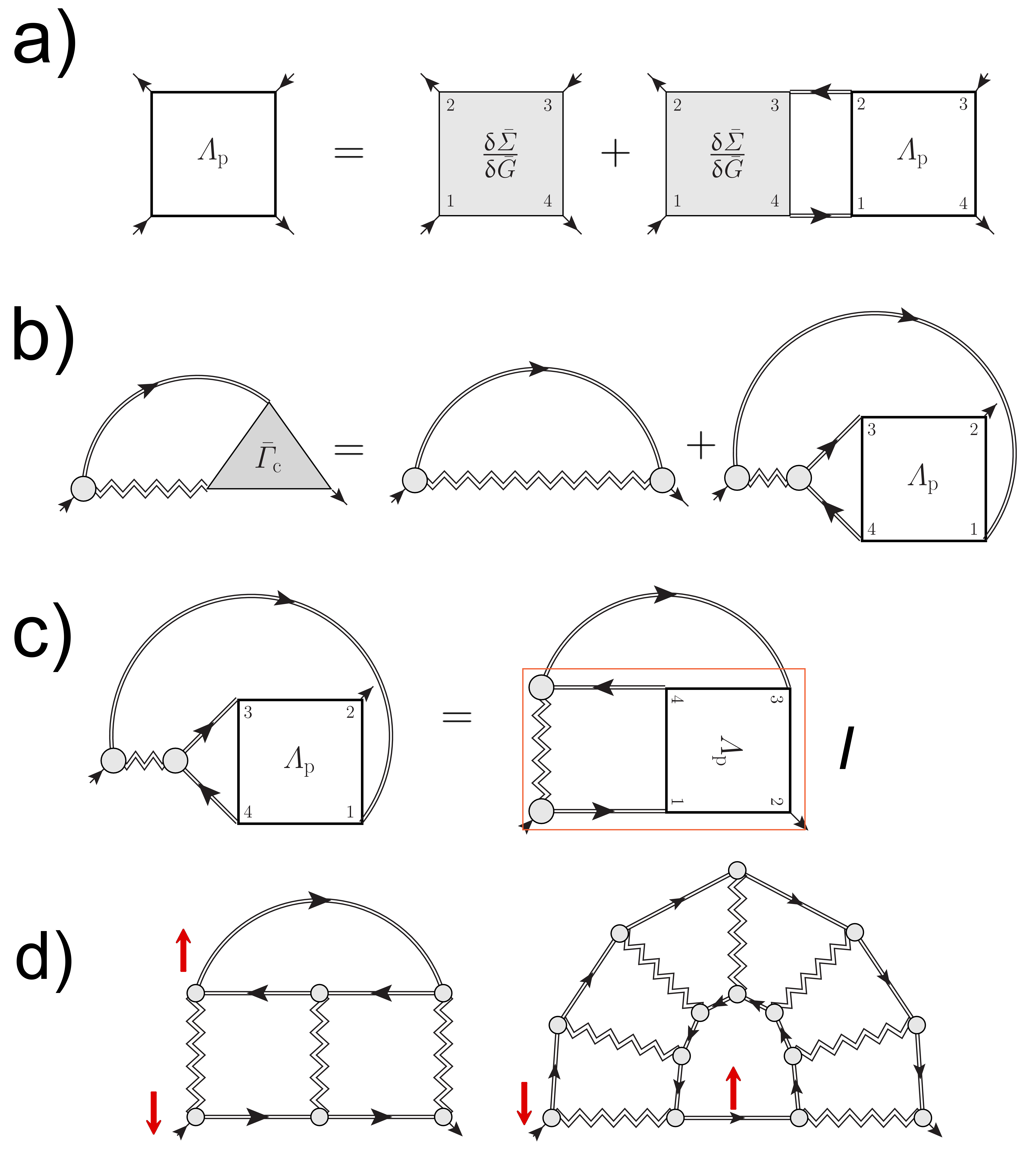
Figure 2: a) Diagrammatic representation of the Dyson equation for the SC particle-hole propagator. b) The electronic self-energy in terms of the particle-hole propagator. c) Interpretation of the vertex part as an exchange diagram with an effective interaction as indicated by the box. d) Contributions to the self-energy from the effective interaction $I$. The arrows indicate that the electrons may have different spin.

Inserting Eq. (LABEL:eq:ElectronicVertexInTermsOfPHProp) into the electronic self-energy Eq. (28) our separation of higher vertex corrections in terms of the particle-hole propagator is complete. The procedure is represented using diagrams as given in Fig. 2 b). As an important fact we realize that the screened interaction $w({\it 1},{\it 2})$ Eq. (30), similar to the bare Coulomb interaction in Hartree-Fock, is independent on spin and the bare vertex conserves angular momentum. Thus, the first self-energy diagram in Fig. 2 b) cannot account for spin flip processes that are discussed as the possible pairing mechanism in the context of High-$T_{{\rm{\scriptscriptstyle c}}}$ superconductivity. The screened Coulomb exchange diagram will, however, contain part of the charge-fluctuations in the sense of the fluctuation-exchange approximation (Bickers et al., 1989). We conclude that angular momentum transfer processes are described by the higher order vertex contributions, i.e. the second diagram of Fig. 2 b). This second self-energy contribution can be twisted to look like an exchange diagram in terms of an effective interaction as indicated by the thin box in Fig. 2 c). In the following we refer to the effective interaction in the box as $I({\it 1}\bar{{\it 1}},{\it 2}\bar{{\it 2}},{\it 3}\bar{{\it 3}},{\it 4}\bar{{\it 4}})$ where we have labeled the degrees of freedom ${\it 1}\bar{{\it 1}},{\it 2}\bar{{\it 2}},{\it 3}\bar{{\it 3}},{\it 4}\bar{{\it 4}}$ starting with ${\it 1}\bar{{\it 1}}$ at the left bottom of the box and then continuing clockwise.

This effective interaction has very interesting properties. For example it can propagate angular momentum and other quantities that are conserved at the bare vertex due to underlying symmetries. This is possible since the diagrams that constitute the effective interaction contain a subset that has no Green’s function connection between “top” (${\it 2}\bar{{\it 2}},{\it 3}\bar{{\it 3}}$) and “bottom” (${\it 1}\bar{{\it 1}},{\it 4}\bar{{\it 4}}$).

An example of such contributions are the horizontal ladder diagrams beyond second order. First and second order are part of the screened Coulomb self-energy and thus have to be excluded to avoid double counting. In this type of diagrams, the conservation at the bare vertex appears independently on the connected top $({\it 2}\bar{{\it 2}}\leftarrow{\it 3}\bar{{\it 3}})$ and bottom (${\it 1}\bar{{\it 1}}\rightarrow{\it 4}\bar{{\it 4}}$) Green’s function lines. Instead, top and bottom are connected only with interaction lines and thus the diagram, viewed as a whole, does not obey the conservation constrains of the bare vertex. Examples of such contributions are given in Fig. 2 d). For the second contribution we have chosen the diagrammatic arrangement of Doniach and Engelsberg (Doniach and Engelsberg, 1966).

For example, a paramagnetic system subject to a Coulomb interaction has a bare vertex that is proportional to $\sigma_{0}$ in spin space. Still, this type of effective interaction in the box of Fig. 2 c) can propagate angular momentum in the sense that it has components proportional to $\sigma_{x,y,z}$ as well, i.e. it describes spin flip processes. Similarly, it also allows to describe how off diagonal Nambu components are rotated due to the interaction. The bare electron-electron and electron-phonon vertex in Nambu space is proportional to $\tau_{z}$ instead of $\sigma_{0}$ as for the spin space, due to the fermionic commutation rules. The box of Fig. 2 c) corresponds to an interaction that has also components in $\tau_{x,y}$ and thus in the language of Anderson (Anderson, 1958) propagates a rotation of iso-spin. These components correspond to the Cooper channel and an interaction mediated by the fluctuation propagator in the sense of Ref. Larkin and Varlamov, 2008.

$I({\it 1}\bar{{\it 1}},{\it 2}\bar{{\it 2}},{\it 3}\bar{{\it 3}},{\it 4}\bar{{\it 4}})$ is a function of four Nambu and spin indices and time and space variables, respectively. We suppress the time and space arguments and decompose $I(\bar{{\it 1}},\bar{{\it 2}},\bar{{\it 3}},\bar{{\it 4}})$ along the Nambu and spin basis

$$I(\bar{{\it 1}},\bar{{\it 2}},\bar{{\it 3}},\bar{{\it 4}}) = \sum_{ijab}I_{ij}^{ab}(\sigma_{a}\tau_{i}\otimes\sigma_{b}\tau_{j})_{\bar{{\it 1}}\bar{{\it 2}}\bar{{\it 3}}\bar{{\it 4}}}$$ (47)

$$I_{ij}^{ab} = \sum_{\bar{{\it 1}}\bar{{\it 2}}\bar{{\it 3}}\bar{{\it 4}}}I(\bar{{\it 1}},\bar{{\it 2}},\bar{{\it 3}},\bar{{\it 4}})(\sigma_{a}\tau_{i})_{\bar{{\it 1}}\bar{{\it 2}}}(\sigma_{b}\tau_{j})_{\bar{{\it 3}}\bar{{\it 4}}}\,.$$ (48)

We write $(\tau_{i}\otimes\tau_{j})_{\bar{{\it 1}}\bar{{\it 2}}\bar{{\it 3}}\bar{{\it 4}}}=(\tau_{i})_{\bar{{\it 1}}\bar{{\it 2}}}(\tau_{j})_{\bar{{\it 3}}\bar{{\it 4}}}$ to indicate that the basis vectors $\tau_{i}$ and $\tau_{j}$ form an outer product. In the following we discuss only the Nambu degrees of freedom since the spin is completely analogue. Considering the Nambu $x,y$ symmetric part of the effective interaction, we may further decompose

$$\sum_{ij=x,y}I_{ij}\tau_{i}\otimes\tau_{j} = I_{-+}(\tau_{x}-{\rm i}\tau_{y})\otimes(\tau_{x}+{\rm i}\tau_{y})+$$ (49)

$$+I_{+-}(\tau_{x}+{\rm i}\tau_{y})\otimes(\tau_{x}-{\rm i}\tau_{y})+$$

$$+I_{++}(\tau_{x}+{\rm i}\tau_{y})\otimes(\tau_{x}+{\rm i}\tau_{y})+$$

$$+I_{--}(\tau_{x}-{\rm i}\tau_{y})\otimes(\tau_{x}-{\rm i}\tau_{y})\bigr{)}$$

with

$$I_{-+} = (I_{xx}+I_{yy}-{\rm i}I_{xy}+{\rm i}I_{yx})/4$$ (50)

$$I_{+-} = (I_{xx}+I_{yy}+{\rm i}I_{xy}-{\rm i}I_{yx})/4$$ (51)

$$I_{++} = (I_{xx}-I_{yy}+{\rm i}I_{xy}+{\rm i}I_{yx})/4$$ (52)

$$I_{--} = (I_{xx}-I_{yy}-{\rm i}I_{xy}-{\rm i}I_{yx})/4$$ (53)

Note that for any complex number $Z$ we find

$$(\tau_{x}\pm{\rm i}\tau_{y})Z = {\rm sign(}\Re Z)|Z|(\tau_{x}\pm{\rm i}\tau_{y}){\rm e}^{\mp{\rm i}\tau_{z}\phi}$$ (54)

$$(\tau_{y}\pm{\rm i}\tau_{z})Z = {\rm sign(}\Re Z)|Z|(\tau_{y}\pm{\rm i}\tau_{z}){\rm e}^{\mp{\rm i}\tau_{x}\phi}$$ (55)

$$(\tau_{z}\pm{\rm i}\tau_{x})Z = {\rm sign(}\Re Z)|Z|(\tau_{z}\pm{\rm i}\tau_{x}){\rm e}^{\mp{\rm i}\tau_{y}\phi}$$ (56)

where $\phi=\text{arctan}(\Im Z/\Re Z)$. Also note that$\tau_{x}{\rm e}^{\mp{\rm i}\tau_{z,y}\phi}={\rm e}^{\pm{\rm i}\tau_{z,y}\phi}\tau_{x}$ and similar for the other Pauli matrices. Thus, we may write

$$(\tau_{x}\pm{\rm i}\tau_{y})\otimes(\tau_{x}\pm{\rm i}\tau_{y})I_{\pm\pm} = {\rm sign(}\Re I_{\pm\pm})|I_{\pm\pm}|\times$$ (57)

$$\times (\tau_{x}\pm{\rm i}\tau_{y}){\rm e}^{\mp{\rm i}\tau_{z}\frac{\phi_{\pm\pm}}{2}}\otimes$$

$$\otimes {\rm e}^{\pm{\rm i}\tau_{z}\frac{\phi_{\pm\pm}}{2}}(\tau_{x}\pm{\rm i}\tau_{y})$$

where

$$\phi_{\pm\pm} = \text{arctan}(\Im I_{\pm\pm}/\Re I_{\pm\pm})\,.$$ (58)

Since the effective interaction $I$ is used in an exchange diagram, we note that $(\tau_{x}\pm{\rm i}\tau_{y})\cdot\bar{G}\cdot(\tau_{x}\pm{\rm i}\tau_{y})$ interchanges the $(\pm 1,\mp 1)$ component of the Green function with the $(\mp 1,\pm 1)$ component in Nambu space. The $(\pm 1,\mp 1)$ component is the complex conjugate of the $(\mp 1,\pm 1)$ component. Such terms $I_{\pm\pm}$, constructed from $I_{xy}^{ab},I_{yx}^{ab},I_{yy}^{ab}$ and $I_{xx}^{ab}$, are the SC analog of a spin flip interaction such as the one of Essenberger et al. (Essenberger et al., ). Furthermore, ${\rm e}^{\mp{\rm i}\tau_{z}\frac{\phi_{\pm\pm}}{2}}\cdot\bar{G}\cdot{\rm e}^{\pm{\rm i}\tau_{z}\frac{\phi_{\pm\pm}}{2}}$ corresponds to a phase rotation of the Nambu off diagonal parts by $\pm\phi_{\pm\pm}$ . Thus, this part of the effective interaction corresponds to a (non-local) phase transformation of the condensate where the phase is rotated by $\pm\phi_{\pm\pm}$ and then conjugated.

In our notation, the spin flip interaction corresponds to the terms $I_{zz}^{xy},I_{zz}^{yx},I_{zz}^{yy}$ and $I_{zz}^{xx}$ since they correspond similarly to a self-energy contribution $\sim(\sigma_{x}\pm{\rm i}\sigma_{y})\cdot\bar{G}\cdot(\sigma_{x}\pm{\rm i}\sigma_{y})$.

VI Summary

We have derived Hedin’s equations for superconducting electrons that are coupled to a system of phonons. Our coupled equations are formally exact. Following the approach of Baym and Kadanoff, we derive the continuity equation for a SC where the external pair potential and its self-energy renormalization appear as source and sink terms for electronic charge. We point out how we can define an effective interaction that can describe fluctuations beyond the screened Coulomb diagram, e.g. of spin of the electrons and phase of condensate. This interaction does not suffer from double counting problems and is given rigorously in terms of the particle-hole propagator.

Acknowledgment

We would like express special thanks to F. Tandetzky and A. Sanna for stimulating discussion and A. Sanna for a careful proof reading of the manuscript.

Appendix A The Electronic Dyson Equation

In this Appendix, we complete the derivation of the Dyson equation Eq. (LABEL:eq:GFDysonEquation). We collect the contributions to the Dyson equation of the single particle parts $\hat{H}_{{\rm{\scriptscriptstyle e}}}+\hat{H}_{{\rm{\scriptscriptstyle aux}}}$ of the total Hamiltonian Eq. (6) on the left hand side of the equation of motion Eq. (14). The commutators ${\rm T}[\hat{H}_{{\scriptscriptstyle{\rm e}-{\rm e}}}+\hat{H}_{{\scriptscriptstyle{\rm e}-{\rm p}}},\hat{\psi}({\it 1}\mu)]$ and ${\rm T}[\hat{H}_{{\scriptscriptstyle{\rm e}-{\rm e}}}+\hat{H}_{{\scriptscriptstyle{\rm e}-{\rm p}}},\hat{\psi}^{\dagger}({\it 1}\mu)]$ are straight forward to evaluate component-wise while the time ordering symbol is essential to cast the result back into the unified notation with the Nambu operators $\hat{\varPsi}({\it 1}\bar{{\it 1}})$. We obtain

$$\sum_{\bar{{\it 3}}}\int{\rm d}{\it 3}\Bigl{(}\delta_{{\it 1},{\it 3}}\bigl{(}\tau_{0}\sigma_{0}\partial_{\tau_{1}}+\sigma_{0}\tau_{z}\varphi({\it 1})\bigl{)}\hat{\bar{H}}_{{\scriptscriptstyle 0}}({\it 1},{\it 3})\Bigr{)}_{\bar{{\it 1}}\bar{{\it 3}}}\times$$ (59)

$$\times \bar{G}({\it{\it 3}}\bar{{\it 3}},{\it 2}\bar{{\it 2}})=$$

$$= \frac{1}{2}\sum_{\bar{{\it{\it 3}}}}\int{\rm d}{\it{\it 3}}w_{{\scriptscriptstyle{\rm 0}}}({\it 1},3)(\sigma_{0}\tau_{z})_{\bar{{\it{\it 3}}},\bar{{\it{\it 3}}}}(\sigma_{0}\tau_{z})_{\bar{{\it 1}},\bar{{\it 1}}}\times$$

$$\times \bar{G}^{{\scriptscriptstyle(2)}}({\it{\it 3}}\bar{{\it{\it 3}}},{\it 1}\bar{{\it 1}},{\it{\it 3}}\bar{{\it{\it 3}}},{\it 2}\bar{{\it 2}})$$

$$- \sum_{\bar{{\it{\it 3}}},q,i}(\bar{v}_{i})_{\bar{{\it 1}}\bar{{\it{\it 3}}}}g_{i}(\boldsymbol{{\it r}}_{1}q)\langle\hat{a}_{q}(\tau_{1})\hat{\varPsi}({\it 1}\bar{{\it{\it 3}}})\hat{\varPsi}^{\dagger}({\it 2}\bar{{\it 2}})\rangle_{{\rm{\scriptscriptstyle T}}}\,.$$

with the two particle Nambu Green’s function $\bar{G}^{{\scriptscriptstyle(2)}}({\it{\it 1}}\bar{{\it{\it 1}}},{\it 2}\bar{{\it 2}},{\it{\it 3}}\bar{{\it{\it 3}}},{\it 4}\bar{{\it 4}})=\langle\hat{\varPsi}^{\dagger}({\it 1}\bar{{\it{\it 1}}})\hat{\varPsi}^{\dagger}({\it 2}\bar{{\it 2}})\hat{\varPsi}({\it 3}\bar{{\it{\it 3}}})\hat{\varPsi}({\it 4}\bar{{\it 4}})\rangle_{{\rm{\scriptscriptstyle T}}}$. Furthermore we derive the relation

$${\rm Tr}_{{\scriptscriptstyle{\rm ns}}}\{\frac{1}{2}\sigma_{0}\tau_{z}\cdot\bar{G}({\it 3},{\it 3})\}\bar{G}({\it 1}\bar{{\it 1}},{\it 2}\bar{{\it 2}})-\frac{\updelta\bar{G}({\it 1}\bar{{\it 1}},{\it 2}\bar{{\it 2}})}{\updelta\varphi({\it 3})}=$$ (60)

$$= \sum_{\bar{{\it 3}}}\frac{1}{2}(\sigma_{0}\tau_{z})_{\bar{{\it 3}},\bar{{\it 3}}}\bar{G}^{{\scriptscriptstyle(2)}}({\it 3}\bar{{\it 3}},{\it 1}\bar{{\it 1}},{\it 3}\bar{{\it 3}},{\it 2}\bar{{\it 2}})\,,$$

and similarly

$$\frac{\updelta\bar{G}({\it 1}\bar{{\it 1}},{\it 2}\bar{{\it 2}})}{\updelta J_{q}(\tau)}-\langle\hat{a}_{q}(\tau_{1})\rangle_{{\rm{\scriptscriptstyle T}}}\bar{G}({\it 1}\bar{{\it 1}},{\it 2}\bar{{\it 2}})=$$

$$\langle\hat{a}_{q}(\tau_{1})\hat{\varPsi}({\it 1}\bar{{\it 1}})\hat{\varPsi}^{\dagger}({\it 2}\bar{{\it 2}})\rangle_{{\rm{\scriptscriptstyle T}}}\,.$$ (61)

Furthermore, for a generic field $A$

$$\frac{\updelta\bar{G}({\it 1},{\it 2})}{\updelta A({\it 3})}=-\bar{G}({\it 1},{\it 4})\cdot\frac{\updelta\bar{G}^{-1}({\it 4},{\it 5})}{\updelta A({\it 3})}\cdot\bar{G}({\it 5},{\it 2})\,.$$ (62)

At this point we introduce the self energy

$$\bar{\varSigma}({\it 1},{\it 2})=$$

$$-w_{{\scriptscriptstyle{\rm 0}}}({\it 1},{\it 3})\tau_{z}\sigma_{0}\cdot\bar{G}({\it 1},{\it 4})\cdot\frac{\updelta\bar{G}^{-1}({\it 4},{\it 2})}{\updelta\varphi({\it 3})}$$

$$-\bar{\varGamma}_{{\scriptscriptstyle{\rm ph}}}^{{\scriptscriptstyle{\rm 0}}}({\it 1},{\it 3};q\tau_{4})\cdot\bar{G}({\it 3},{\it 4})\cdot\frac{\updelta\bar{G}^{-1}({\it 4},{\it 2})}{\updelta J_{q}(\tau_{4})}+$$

$$+\bar{\varGamma}_{{\scriptscriptstyle{\rm ph}}}^{{\scriptscriptstyle{\rm 0}}}({\it 1},{\it 3};q\tau_{4})\cdot\updelta_{{\it 2},{\it 3}}\sigma_{0}\tau_{0}\langle\hat{a}_{q}(\tau_{4})\rangle\,.$$ (63)

Inserting the Eqs. (60) and (61) into Eq. (59), together with the definition of the Hartree Hamiltonian $\hat{\bar{H}}_{{\rm{\scriptscriptstyle H}}}({\it 1},{\it 3})$, we arrive at

$$\int{\rm d}{\it 3}\bigl{(}-\delta_{{\it 1},{\it 3}}\tau_{0}\sigma_{0}\partial_{\tau_{1}}-\hat{\bar{H}}_{{\scriptscriptstyle{\rm H}}}({\it 1},{\it 3})\bigr{)}\cdot\bar{G}({\it 3},{\it 2})$$

$$=\updelta_{{\it 1}{\it 2}}\updelta_{\bar{{\it 1}}\bar{{\it 2}}}+\int{\rm d}{\it 3}\bar{\varSigma}({\it 1},{\it 3})\cdot\bar{G}({\it 3},{\it 2})\,.$$ (64)

Now we insert $\bar{G}_{{\scriptscriptstyle{\rm H}}}\bar{G}_{{\scriptscriptstyle{\rm H}}}^{-1}$ and with the Hartree Green’s function Eq. (LABEL:eq:HartreeGreensfunction), applying $\bar{G}_{{\scriptscriptstyle{\rm H}}}$ from the left, we arrive at Eq. (LABEL:eq:GFDysonEquation).

Appendix B Conservation conditions for the Green Function

In this Appendix, we want to discuss the conditions implied by the Dyson equation for the electronic Green function Eq. (LABEL:eq:GFDysonEquation). We give the non-local basic equation, that we use to derive the continuity equation. The procedure is a straight forward adaption of Baym and Kadanoff(Baym and Kadanoff, 1961), noting that $\bar{G}_{{\rm{\scriptscriptstyle 0}}}^{-1}$ and $\bar{G}$ are $4\times 4$ matrices that do not commute. The result for the left hand side of Eq. (35) is

$$\int{\rm d}{\it 3}\bigl{(}\bar{G}_{{\rm{\scriptscriptstyle 0}}}^{-1}({\it 1},{\it 3})\cdot\bar{G}({\it{\it 3}},{\it 2})-\bar{G}({\it{\it 1}},{\it 3})\cdot\bar{G}_{{\rm{\scriptscriptstyle 0}}}^{-1}({\it 3},{\it 2})\bigr{)}=$$ (65)

$$= \Bigl{(}-\sigma_{0}\tau_{0}(\partial_{\tau_{1}}+\partial_{\tau_{2}})-\sigma_{0}\tau_{z}\frac{1}{2}\bigl{(}-{\rm i}(\boldsymbol{\nabla}_{\boldsymbol{r}_{1}}+\boldsymbol{\nabla}_{\boldsymbol{r}_{2}})+\boldsymbol{A}_{{\scriptscriptstyle{\rm ext}}}({\it 1})-\boldsymbol{A}_{{\scriptscriptstyle{\rm ext}}}({\it 2})\bigr{)}\bigl{(}-{\rm i}(\boldsymbol{\nabla}_{\boldsymbol{r}_{1}}-\boldsymbol{\nabla}_{\boldsymbol{r}_{2}})+\boldsymbol{A}_{{\scriptscriptstyle{\rm ext}}}({\it 1})+\boldsymbol{A}_{{\scriptscriptstyle{\rm ext}}}({\it 2})\bigr{)}$$

$$+ \sigma_{0}\tau_{z}\bigl{(}\phi_{{\scriptscriptstyle{\rm ext}}}({\it 1})-\phi_{{\scriptscriptstyle{\rm ext}}}({\it 2})\bigr{)}+\frac{1}{2}\bigl{(}\mathbf{S}(\tau_{0}+\tau_{z})-\mathbf{S}^{\ast}(\tau_{0}-\tau_{z})\bigr{)}\cdot\bigl{(}\boldsymbol{B}_{{\scriptscriptstyle{\rm ext}}}({\it 1})-\boldsymbol{B}_{{\scriptscriptstyle{\rm ext}}}({\it 2})\bigr{)}\Bigr{)}\cdot\bar{G}({\it{\it 1}},{\it 2})$$

$$- \Bigl{(}\bigl{(}{\rm i}\boldsymbol{\nabla}_{\boldsymbol{r}_{2}}+\boldsymbol{A}_{{\scriptscriptstyle{\rm ext}}}({\it 2})\bigr{)}^{2}+\phi_{{\scriptscriptstyle{\rm ext}}}({\it 2})\Bigr{)}[\sigma_{0}\tau_{z},\bar{G}({\it{\it 1}},{\it 2})]-\frac{1}{2}[\bigl{(}\mathbf{S}(\tau_{0}+\tau_{z})-\mathbf{S}^{\ast}(\tau_{0}-\tau_{z})\bigr{)}\cdot\boldsymbol{B}_{{\scriptscriptstyle{\rm ext}}}({\it 2}),\bar{G}({\it{\it 1}},{\it 2})]$$

$$+ \frac{1}{2}\int{\rm d}{\it 3}\bigl{(}(\tau_{x}-{\rm i}\tau_{y})\boldsymbol{\varDelta}_{{\scriptscriptstyle{\rm ext}}}({\it 1},{\it 3})\cdot\boldsymbol{\Phi}-(\tau_{x}+{\rm i}\tau_{y})\boldsymbol{\varDelta}_{{\scriptscriptstyle{\rm ext}}}^{\ast}({\it 1},{\it 3})\cdot\boldsymbol{\Phi}\bigr{)}\cdot\bar{G}({\it{\it 3}},{\it 2})$$

$$- \frac{1}{2}\int{\rm d}{\it 3}\bar{G}({\it{\it 1}},{\it 3})\cdot\bigl{(}(\tau_{x}-{\rm i}\tau_{y})\boldsymbol{\varDelta}_{{\scriptscriptstyle{\rm ext}}}({\it 3},{\it 2})\cdot\boldsymbol{\Phi}-(\tau_{x}+{\rm i}\tau_{y})\boldsymbol{\varDelta}_{{\scriptscriptstyle{\rm ext}}}^{\ast}({\it 3},{\it 2})\cdot\boldsymbol{\Phi}\bigr{)}$$

The Nambu off diagonal right hand side of Eq. (35) is then evaluated to be

$$\frac{1}{2}\int{\rm d}{\it 3}\bigl{(}(\tau_{x}+{\rm i}\tau_{y})\bar{\varSigma}({\it 1},1,{\it 3},-1)+(\tau_{x}-{\rm i}\tau_{y})\bar{\varSigma}({\it 1},-1,{\it 3},1)\bigr{)}\cdot\bar{G}({\it{\it 3}},{\it 1})$$ (71)

$$- \frac{1}{2}\int{\rm d}{\it 3}\bar{G}({\it{\it 1}},{\it 3})\cdot\bigl{(}(\tau_{x}+{\rm i}\tau_{y})\bar{\varSigma}({\it 3},1,{\it 2},-1)+(\tau_{x}-{\rm i}\tau_{y})\bar{\varSigma}({\it 3},-1,{\it 2},1)\bigr{)}$$

$$= \left(\begin{array}[]{cc}\mathfrak{Im}\bigl{\{}\int{\rm d}{\it 3}\mathfrak{Re}\{\bar{\varSigma}({\it 1},1,{\it 3},-1)\}\bar{G}({\it{\it 3}},-1,{\it 2},1)\bigr{\}}&\mathfrak{Re}\bigl{\{}\int{\rm d}{\it 3}\mathfrak{Re}\{\bar{\varSigma}({\it 1},1,{\it 3},-1)\}\bar{G}({\it{\it 3}},-1,{\it 2},-1)\bigr{\}}\\ \mathfrak{Re}\bigl{\{}\int{\rm d}{\it 3}\mathfrak{Re}\{\bar{\varSigma}({\it 1},-1,{\it 3},1)\}\bar{G}({\it{\it 3}},1,{\it 2},1)\bigr{\}}&\mathfrak{Im}\bigl{\{}\int{\rm d}{\it 3}\mathfrak{Re}\{\bar{\varSigma}({\it 1},-1,{\it 3},1)\}\bar{G}({\it{\it 3}},1,{\it 2},-1)\bigr{\}}\end{array}\right)$$

$$+\left(\begin{array}[]{cc}\mathfrak{Re}\bigl{\{}\int{\rm d}{\it 3}\mathfrak{Im}\{\bar{\varSigma}({\it 1},1,{\it 3},-1)\}\bar{G}({\it{\it 3}},-1,{\it 2},1)\bigr{\}}&\mathfrak{Im}\bigl{\{}\int{\rm d}{\it 3}\mathfrak{Im}\{\bar{\varSigma}({\it 1},1,{\it 3},-1)\}\bar{G}({\it{\it 3}},-1,{\it 2},-1)\bigr{\}}\\ \mathfrak{Im}\bigl{\{}\int{\rm d}{\it 3}\mathfrak{Im}\{\bar{\varSigma}({\it 1},-1,{\it 3},1)\}\bar{G}({\it{\it 3}},1,{\it 2},1)\bigr{\}}&\mathfrak{Re}\bigl{\{}\int{\rm d}{\it 3}\mathfrak{Im}\{\bar{\varSigma}({\it 1},-1,{\it 3},1)\}\bar{G}({\it{\it 3}},1,{\it 2},-1)\bigr{\}}\end{array}\right)\,.$$

The Nambu diagonal part can be computed in an analogous way. Taking the local limit ${\it 2}\rightarrow{\it 1}$ of the Eq. (65) gives

$$\int{\rm d}{\it 3}\bigl{(}\bar{G}_{{\rm{\scriptscriptstyle 0}}}^{-1}({\it 1},{\it 3})\cdot\bar{G}({\it{\it 3}},{\it 1})-\bar{G}({\it{\it 1}},{\it 3})\cdot\bar{G}_{{\rm{\scriptscriptstyle 0}}}^{-1}({\it 3},{\it 1})\bigr{)}=$$ (72)

$$= \Bigl{(}-2\sigma_{0}\tau_{0}\partial_{\tau_{1}}\bar{G}({\it{\it 1}},{\it 2})|_{{\it 2}\rightarrow{\it 1}}+2\sigma_{0}\tau_{z}{\rm i}\boldsymbol{\nabla}_{\boldsymbol{r}_{1}}\bigl{(}\frac{1}{2{\rm i}}(\boldsymbol{\nabla}_{\boldsymbol{r}_{1}}-\boldsymbol{\nabla}_{\boldsymbol{r}_{2}})+\boldsymbol{A}_{{\scriptscriptstyle{\rm ext}}}({\it 1})\bigr{)}\bar{G}({\it{\it 1}},{\it 2})|_{{\it 2}\rightarrow{\it 1}}$$

$$- \Bigl{(}\bigl{(}{\rm i}\boldsymbol{\nabla}_{\boldsymbol{r}_{2}}+\boldsymbol{A}_{{\scriptscriptstyle{\rm ext}}}({\it 1})\bigr{)}^{2}+\phi_{{\scriptscriptstyle{\rm ext}}}({\it 1})\Bigr{)}[\sigma_{0}\tau_{z},\bar{G}({\it{\it 1}},{\it 2})]|_{{\it 2}\rightarrow{\it 1}}-\frac{1}{2}[\bigl{(}\mathbf{S}(\tau_{0}+\tau_{z})-\mathbf{S}^{\ast}(\tau_{0}-\tau_{z})\bigr{)}\cdot\boldsymbol{B}_{{\scriptscriptstyle{\rm ext}}}({\it 1}),\bar{G}({\it{\it 1}},{\it 1})]$$

$$+ \frac{1}{2}\int{\rm d}{\it 3}\bigl{(}(\tau_{x}+{\rm i}\tau_{y})\boldsymbol{\varDelta}_{{\scriptscriptstyle{\rm ext}}}({\it 1},{\it 3})\cdot\boldsymbol{\Phi}-(\tau_{x}-{\rm i}\tau_{y})\boldsymbol{\varDelta}_{{\scriptscriptstyle{\rm ext}}}^{\ast}({\it 1},{\it 3})\cdot\boldsymbol{\Phi}\bigr{)}\cdot\bar{G}({\it{\it 3}},{\it 1})$$

$$- \frac{1}{2}\int{\rm d}{\it 3}\bar{G}({\it{\it 1}},{\it 3})\cdot\bigl{(}(\tau_{x}+{\rm i}\tau_{y})\boldsymbol{\varDelta}_{{\scriptscriptstyle{\rm ext}}}({\it 3},{\it 1})\cdot\boldsymbol{\Phi}-(\tau_{x}-{\rm i}\tau_{y})\boldsymbol{\varDelta}_{{\scriptscriptstyle{\rm ext}}}^{\ast}({\it 3},{\it 1})\cdot\boldsymbol{\Phi}\bigr{)}\,.$$

It is important that the commutator $[\sigma_{0}\tau_{z},\bar{G}({\it{\it 3}},{\it 2})]$ has only components on the Nambu off diagonal. If we are interested in the usual conservation laws of electronic charge or magnetic density, these terms do not appear. Taking the local limit and selecting only the $1,1$ component, the equations simplify significantly and we arrive at Eq. (36).

Furthermore, we point out that if the self-energy is non-SC, i.e. has only Nambu diagonal non vanishing components$\bar{\varSigma}({\it 1},{\it 3})\propto\tau_{z},\tau_{0}$, the right hand side of Eq. (35) is proportional to the commutator $[\sigma_{0}\tau_{z},\bar{G}({\it{\it 3}},{\it 2})]$. This commutator on the other hand does not have components on the Nambu diagonal, i.e. the usual continuity equations for electronic charge and magnetic density are satisfied without self-energy contributions as expected.