The degree of mobility of Einstein metrics

Abstract.

Two pseudo-Riemannian metrics are called projectively equivalent if their unparametrized geodesics coincide. The degree of mobility of a metric is the dimension of the space of metrics that are projectively equivalent to it. We give a complete list of possible values for the degree of mobility of Riemannian and Lorentzian Einstein metrics on simply connected manifolds, and describe all possible dimensions of the space of essential projective vector fields.

1. Introduction

The aim of this article is to study Einstein metrics (i.e., such that the Ricci curvature is proportional to the metric) of Riemannian and Lorentzian signature in the realm of projective geometry.

Recall that two pseudo-Riemannian metrics $g$ and $\bar{g}$ on a manifold $M$ are called projectively equivalent if their unparametrized geodesics coincide. Clearly, any constant multiple of $g$ is projectively equivalent to $g$. A generic metric does not admit other examples of projectively equivalent metrics, see [27]. If two metrics $g,\bar{g}$ are affinely equivalent, that is, if their Levi-Civita connections coincide, then they are also projectively equivalent. Affinely equivalent metrics are well-understood at least in Riemannian [12, 15] and Lorentzian signature [26, 34], see also Lemma 9 below. The case of arbitrary signature is much more complicated, see [26] or the more recent article [5] for a local description of all such metrics.

The theory of projectively equivalent metrics has a long and rich history – we refer to the introductions of [25, 29] or to survey [33] for more details, and focus on Einstein metrics in what follows.

Einstein metrics are very natural objects in projective geometry. For instance, as shown in [25], the property of a metric $g$ to be Einstein is projectively invariant in the following sense: any metric that projectively equivalent and not affinely equivalent to an Einstein metric is also Einstein. A more educated point of view on the whole subject is the following: a projective geometry, given by a class of projectively equivalent connections (not necessarily Levi-Civita connections), is an example of a parabolic geometry, a special case of a Cartan geometry, see the monographs [10, 35]. As shown in [18], the metrics with Levi-Civita connection contained in the given projective class are in one-one correspondence to solutions of a certain overdetermined system of partial differential equations. This system is a so-called first Bernstein-Gelfand-Gelfand equation [6, 11] and, as shown in [7], Einstein metrics correspond to a special class of solutions called normal.

The degree of mobility $D(g)$ of a pseudo-Riemannian metric $g$ is the dimension of the space of $g$-symmetric solutions of the PDE (2). As we explain in Section 2, nondegenerate solutions of (2) are in one-to-one correspondence with the metrics projectively equivalent to $g$. Hence, intuitively, $D(g)$ is the dimension of the space of metrics projectively equivalent to $g$.

We have $D(g)=1$ for a generic metric $g$ and $D(g)\geq 2$ if $g$ admits a projectively equivalent metric that is nonproportional to $g$. As our main result, we determine all possible values for the degree of mobility $D(g)$ of Riemannian and Lorentzian Einstein metrics, locally or on simply connected manifolds. Let us denote by “$[\alpha]$” the integer part of a real number $\alpha$.

Theorem 1.

Let $(M,g)$ be a simply connected Riemannian or Lorentzian Einstein manifold of dimension $n\geq 3$. Suppose $g$ admits a projectively equivalent but not affinely equivalent metric.

Then, the degree of mobility $D(g)$ is one of the numbers $\geq 2$ from the following list:

• $\frac{k(k+1)}{2}+l$, where $n\geq 5$, $0\leq k\leq n-4$ and $1\leq l\leq[\frac{n+1-k}{5}]$ for $g$ Riemannian and Lorentzian.

• $\frac{k(k+1)}{2}+l$, where $n\geq 5$, $k=n-3\mbox{ mod }5$, $2\leq k\leq n-3$ and $l=[\frac{n+2-k}{5}]$ for $g$ Lorentzian.

• $\frac{(n+1)(n+2)}{2}$.

Conversely, for $n\geq 3$ and each number $D\geq 2$ from this list, there exist simply connected $n$-dimensional Riemannian resp. Lorentzian Einstein manifolds admitting projectively equivalent but not affinely equivalent metrics and such that $D$ is the degree of mobility $D(g)$.

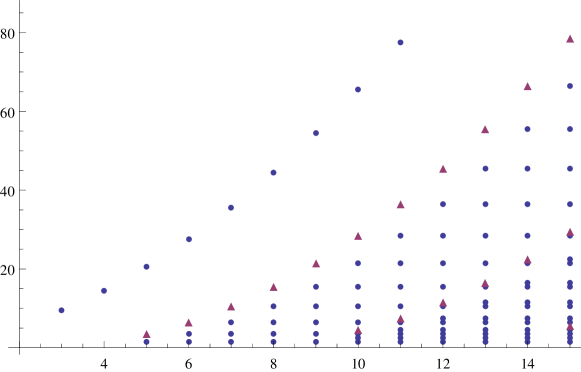
Figure 1. Degree of mobility $D(g)$ from Theorem 1 for $3\leq\mathrm{dim}\,M\leq 15$. The triangles denote the additional values for Lorentz signature.

In Theorem 1, the degree of mobility is at least $2$ since we assumed that $g$ admits a metric $\bar{g}$ projectively equivalent to $g$ but not affinely equivalent to it. Suppose this assumption is dropped, that is, let us assume all metrics projectively equivalent to $g$ are affinely equivalent to it. In this case the complete list of possible values of the degree of mobility of $g$ can be easily obtained by combining Lemma 9 below with methods similar to the ones used in Section 3.2 and Section 3.4. It is

$$\{k(k+1)/2+l:0\leq k\leq n-2,1\leq l\leq[(n-k)/2]\}\cup\{n(n+1)/2\}$$

if $g$ is Einstein with nonzero scalar curvature and

$$\{k(k+1)/2+l:0\leq k\leq n-4,1\leq l\leq[(n-k)/4]\}\cup\{n(n+1)/2\}$$

if $g$ is Ricci flat.

It is well-known, see e.g. [37, p.134], that if $D(g)$ is equal to its maximal value $(n+1)(n+2)/2$, then $g$ has constant sectional curvature. Conversely, this value is attained on simply connected manifolds of constant sectional curvature. In view of this, the case $n=3$ in Theorem 1 is trivial, since a $3$-dimensional Einstein metric has constant sectional curvature and its degree of mobility takes the maximum value $D(g)=10$.

For $4$-dimensional Einstein metrics, we obtain the following statement as an immediate consequence of Theorem 1 (compare also Figure 1):

Corollary 2.

Let $(M,g)$ be a $4$-dimensional Riemannian or Lorentzian Einstein manifold. Suppose $\bar{g}$ is projectively equivalent to $g$ but not affinely equivalent. Then, $g$ has constant sectional curvature.

Corollary 2 was known before, see [25, Theorem 2] (or, alternatively, [22]), and it is actually true for metrics of arbitrary signature. However, our methods for proving Theorem 1 and Corollary 2 are different from that used in [22, 25] (although we will rely on some statements from [25]). A special case of Corollary 2 was also considered in [34] where it was proven that $4$-dimensional Ricci flat nonflat metrics cannot be projectively equivalent unless they are affinely equivalent. This result was generalized to Einstein metrics of arbitrary scalar curvature in [21]. Note that by [25, Theorem 1], the statement of Corollary 2 survives for arbitrary dimension under the assumption that both metrics are geodesically complete.

Projective equivalence of Lorentzian Einstein metrics, in particular, the problem we have investigated, was actively studied in general relativity, see the classical references [14, 16, 38] and the more recent articles [21, 22, 27]. The motivation to study this problem is based on the description of trajectories of freely falling particles in vacuum as unparametrized geodesics of a Lorentzian Einstein metric. The initial question, studied in [19, 34, 38], is whether and under what conditions one can reconstruct the spacetime metric by only observing freely falling particles. We study the ‘freedom’ of such a reconstruction: the number of parameters is given by Theorem 1.

We see from Theorem 1 that the list for the values of the degree of mobility for Riemannian Einstein metrics is strictly smaller than the list for Lorentzian Einstein metrics. This difference starts in dimension five: for a $5$-dimensional Riemannian Einstein metric $g$ we have $D(g)=1,2$ or $g$ has constant sectional curvature (i.e., $D(g)=21$). However, according to Theorem 1, there exist $5$-dimensional Lorentzian Einstein metrics having $D(g)=4$. For instance, consider

Example 1.

The nonconstant curvature metric

$$g=\mathrm{d}t^{2}+e^{2t}(\mathrm{d}x_{0}\odot\mathrm{d}x_{1}+e^{x_{2}}\mathrm{sin}(x_{3})\mathrm{d}x_{1}^{2}+\mathrm{d}x_{2}^{2}+\mathrm{d}x_{3}^{2})$$

on $M=\mathbb{R}^{5}$ (with coordinates $(t,x_{0},x_{1},x_{2},x_{3})$) is Einstein with scalar curvature $20$ and has signature $(1,4)$. In addition to $g$, the following symmetric $(0,2)$-tensors are solutions of equation (2):

$$L_{1}=e^{2t}\mathrm{d}t^{2},\,\,\,L_{2}=e^{2t}(x_{1}\mathrm{d}t+\mathrm{d}x_{1})^{2},\,\,\,L_{3}=e^{2t}\mathrm{d}t\odot(x_{1}\mathrm{d}t+\mathrm{d}x_{1}).$$

Without the assumption that the metric is Einstein, an analogue of Theorem 1 is [20, Theorem 1]. Obviously, the values obtained in Theorem 1 are contained in the list of [20, Theorem 1], but our list is of course thinner: not every value from [20, Theorem 1] can be realized as the degree of mobility of an Einstein metric. We suggest to compare Figure 1 above with [20, Fig. 1].

Note also that most experts (including us) expected that the list for the values of the degree of mobility should not depend on the signature. This is true (at least when comparing Riemannian and Lorentzian signature) if we do consider general metrics (not necessarily Einstein), see [20, Theorem 1]. As stated in Theorem 1, it is not true when we consider Einstein metrics, see also Example 1 above.

Note that if the manifold is closed, the list of possible values for the degree of mobility is much shorter. Indeed, by [25, 30], a metric that is projectively equivalent to an Einstein metric of nonconstant sectional curvature on a closed manifold is affinely equivalent to it.

1.1. Application: the dimension of the space of essential projective vector fields

Let $(M,g)$ be a pseudo-Riemannian manifold. A diffeomorphism $f:M\rightarrow M$ is called a projective transformation if it maps unparametrized geodesics to unparametrized geodesics or, equivalently, if $f^{*}g$ is projectively equivalent to $g$. The isometries of $g$ are clearly projective transformations. A projective transformation is called essential if it is not an isometry of the metric.

A vector field $v$ on $(M,g)$ is called projective if its local flow consists of projective transformations. A projective vector field is called essential if it is not a Killing vector field.

Let $\mathfrak{p}(g)$ and $\mathfrak{i}(g)$ denote the vector spaces (in fact, Lie algebras) of projective and Killing vector fields respectively. The quotient $\mathfrak{p}(g)/\mathfrak{i}(g)$ will be referred to as the space of essential projective vector fields. In the generic case, see Remark 6 below, this space can be naturally identified with a subspace (thought, not a subalgebra) of $\mathfrak{p}(g)$.

We determine all possible values for the dimension of the space of essential projective vector fields of a Riemannian or Lorentzian Einstein metric:

Theorem 3.

Let $(M,g)$ be a simply connected Riemannian or Lorentzian Einstein manifold of dimension $n\geq 3$ which admits a metric that is projectively equivalent but not affinely equivalent to $g$. Then, the possible values for the dimension of the space of essential projective vector fields are given by the numbers $\geq 1$ from the following list:

• $\frac{k(k+1)}{2}+l-1$, where $n\geq 5$, $0\leq k\leq n-4$ and $1\leq l\leq[\frac{n+1-k}{5}]$ for $g$ Riemannian and Lorentzian.

• $\frac{k(k+1)}{2}+l-1$, where $n\geq 5$, $k=n-3\mbox{ mod }5$, $2\leq k\leq n-3$ and $l=[\frac{n+2-k}{5}]$ for $g$ Lorentzian.

• $\frac{(n+1)(n+2)}{2}-1$.

Conversely, for $n\geq 3$ and each number $\geq 1$ from this list, there exists a $n$-dimensional simply connected Riemannian resp. Lorentzian Einstein metric admitting a projectively equivalent but not affinely equivalent metric and for which this number is the dimension of the space of essential projective vector fields.

Comparing the list from Theorem 3 with that in Theorem 1, we see that the possible values for $\mathrm{dim}\left(\mathfrak{p}(g)/\mathfrak{i}(g)\right)$ are given by the values for the degree of mobility $D(g)$ subtracted by $1$. Indeed, in the generic case, the number of essential projective vector fields of an Einstein metric is $D(g)-1$. Moreover, if in addition to our assumptions the metric is Riemannian or the scalar curvature is not zero, then there exists a natural linear mapping with $1$-dimensional kernel from the set of solutions of (2) to the space $\mathfrak{p}(g)/\mathfrak{i}(g)$, see Section 4.1 below. There exist though Einstein metrics of Lorentzian signature such that $\mathrm{dim}\left(\mathfrak{p}(g)/\mathfrak{i}(g)\right)<D(g)-1$.

By Theorem 3, any Einstein metric of Riemannian or Lorentzian signature admitting a nonaffinely equivalent projectively equivalent metric also admits an essential projective vector field. The next theorem shows that the assumption on signature is not essential.

Theorem 4.

Let $g$ be an Einstein metric of arbitrary signature on a simply connected manifold of dimension $n\geq 3$. If there exists a metric that is projectively equivalent but not affinely equivalent to $g$, there exists at least one essential projective vector field for $g$.

Examples show that the assumption that the metric is Einstein is essential for Theorem 4.

As we already recalled above, an Einstein metric of arbitrary signature and of nonconstant sectional curvature on a closed manifold does not admit projectively but not affinely equivalent metrics. Therefore, on a closed Einstein manifold of nonconstant sectional curvature every projective transformation is an affine transformation and, hence, every projective vector field is an affine vector field. Actually, in the Riemannian case we do not need the assumption that the metric is Einstein in the latter statement, see [28, Corollary 1].

Similar results were also obtained in the case the manifold is not necessarily closed but under the additional assumption that the metric $g$ and a projectively equivalent but not affinely equivalent metric $\bar{g}$ are complete. By [25, Theorem 1], projective but not affine equivalence of two complete metrics (of arbitrary signature) one of which is Einstein implies that both metrics have constant sectional curvature. This implies that complete Einstein metrics do not admit complete projective but not affine vector fields. Again in the Riemannian case we do not need the assumption that the metric is Einstein in the latter statement, see [28, Theorem 1].

Note that the result of Theorem 3 has a predecessor: in [20, Theorem 3] the possible dimensions of the space of essential projective vector fields have been determined for a general Riemannian or Lorentzian metric. As before the list of values we have obtained in the Einstein case is shorter than the list of values obtained in [20, Theorem 3].

1.2. Organisation of the article

In Section 2, we recall basic facts from the theory of projectively equivalent metrics.

The remaining sections deal with the proofs of the Theorems 1, 3 and 4. As mentioned above, the case of general (= not necessarily Einstein) metrics was solved in [20]. We extensively use and therefore quote necessary results from [20] in the paper and indicate the places when the additional condition that the metric is Einstein becomes important.

The proof of Theorem 1 will be given in Section 3. It is divided into several parts and a rough discription of how we proceed can be found in Section 3.1.

The proof of Theorem 3 and that of Theorem 4 will be given in Section 4.

2. Basic formulas

Let $g,\bar{g}$ be two pseudo-Riemannian metrics on an $n$-dimensional manifold $M$. We define a symmetric nondegenerate $(0,2)$-tensor $L$ by

(1) $$L=L(g,\bar{g})=\Big{|}\frac{\mathrm{det}\,\bar{g}}{\mathrm{det}\,g}\Big{|}^{\frac{1}{n+1}}g\bar{g}^{-1}g.$$

In the formula above, we view $g,\bar{g}:TM\rightarrow T^{*}M$ naturally as bundle isomorphisms and identify $(0,2)$-tensors with endomorphism $TM\rightarrow T^{*}M$ via $L(X)(Y)=L(X,Y)$ for $X,Y\in TM$. In tensor notation, (1) reads

$$L_{ij}=\Big{|}\frac{\mathrm{det}\,\bar{g}}{\mathrm{det}\,g}\Big{|}^{\frac{1}{n+1}}g_{ik}\bar{g}^{kl}g_{lj},$$

where $\bar{g}^{ik}\bar{g}_{kj}=\delta^{i}_{j}$. It is a fundamental fact, see [36], that $g$ and $\bar{g}$ are projectively equivalent, if and only if the tensor $L$ from (1) is a solution to the following PDE

(2) $$\nabla_{X}L=X^{\flat}\odot\Lambda,\,\,\,X\in TM,$$

where $\Lambda$ is a certain $1$-form, $\nabla$ denotes the Levi-Civita connection of $g$, $\alpha\odot\beta=\alpha\otimes\beta+\beta\otimes\alpha$ for $1$-forms $\alpha,\beta$ and $X^{\flat}=g(X,.)$ denotes the metric dual w.r.t. $g$.

Throughout the article, when it is clear which metric is used, we will denote by $X^{\flat}\in T^{*}M$ the metric dual of a vector $X\in TM$ and by $\alpha^{\sharp}\in TM$ the metric dual of a $1$-form $\alpha\in T^{*}M$. Similarly, for a $(0,2)$-tensor $L$ we let $L^{\sharp}$ denote the corresponding $(1,1)$-tensor defined by $g(L^{\sharp}.,.)=L$.

Taking a trace in (2) using $g$ shows that

$$\Lambda=\mathrm{d}\lambda\mbox{, where }\lambda=\frac{1}{2}\mathrm{trace}(L^{\sharp}).$$

Thus, (2) is in fact a linear PDE of first order on symmetric $(0,2)$-tensors $L$. As stated above, the nondegenerate symmetric solutions of (2) correspond via (1) to metrics projectively equivalent to $g$. In fact, if $L$ is such a solution then $\bar{g}=(\mathrm{det}\,L^{\sharp})^{-1}g((L^{\sharp})^{-1}.,.)$ is projectively equivalent to $g$. Since $g$ is always a solution of (1) (corresponding to the fact that $g$ is projectively equivalent to itself), we can (locally) make any symmetric solution of (2) nondegenerate by adding a suitable multiple of $g$. In this sense the linear space of symmetric solutions of (2) corresponds to the space of metrics being projectively equivalent to $g$.

Definition.

Let $(M,g)$ be a pseudo-Riemannian manifold. We denote by $\mathcal{A}(g)$ the linear space of symmetric solutions of (2). The degree of mobility $D(g)$ of $g$ is the dimension of $\mathcal{A}(g)$.

In view of the above correspondence we will often consider a pair $g,L$, where $L\in\mathcal{A}(g)$, instead of a pair $g,\bar{g}$ of projectively equivalent metrics.

As stated in the introduction, affinely equivalent metrics (i.e. metrics having the same Levi-Civita connections) are projectively equivalent. Obviously, two metrics $g,\bar{g}$ are affinely equivalent if and only if the tensor $L=L(g,\bar{g})$ from (1) is parallel (w.r.t. the Levi-Civita connection of one of the metrics). In view of (2), this is equivalent to the property that $\Lambda$ from (2) is identically zero. Combining these, we obtain the following wellknown statement:

Lemma 5.

Let $g,\bar{g}$ be projectively equivalent pseudo-Riemannian metrics on a manifold $M$ and let $L=L(g,\bar{g})\in\mathcal{A}(g)$ be given by (1). Then, $g,\bar{g}$ are affinely equivalent if and only if $L$ is $g$-parallel if and only if the $1$-form $\Lambda$ corresponding to $L$ is identically zero.

Of fundamental importance for our goals is the following

Theorem 6.

[25] Let $(M,g)$ be a connected pseudo-Riemannian Einstein manifold of dimension $n\geq 3$ such that at least one $L\in\mathcal{A}(g)$ is nonparallel. Let

$$B=-\frac{\mathrm{Scal}}{n(n-1)},$$

where $\mathrm{Scal}$ denotes the scalar curvature of $g$.

Then, for every $L\in\mathcal{A}(g)$ with corresponding $1$-form $\Lambda$, there exists a function $\mu$ such that $(L,\Lambda,\mu)$ satisfies

(3) $$\nabla_{X}L=X^{\flat}\odot\Lambda,\,\,\,\nabla\Lambda=\mu g+BL,\,\,\,\nabla\mu=2B\Lambda.$$

Remark 1.

Theorem 6 follows from [25, Corollary 1 and 2]. As shown in [24], under the assumption $D(g)\geq 3$, the statement is actually true for any metric (not necessarily Einstein) and a certain constant $B$ (which is not necessarily equal to $-\mathrm{Scal}/n(n-1)$ in this case).

3. Proof of Theorem 1

3.1. Scheme of the proof

By Theorem 6, under the assumptions of Theorem 1, the degree of mobility $D(g)$ equals the dimension of the space of solutions of the system (3). The proof of Theorem 1 is different for $B=-\mathrm{Scal}/n(n-1)=0$ and for $B\neq 0$.

Consider first the case $B\neq 0$. By scaling the metric $g$ we may assume that $B=-1$. The key observation is that for $B=-1$ the solutions of the system (3) correspond to parallel symmetric $(0,2)$-tensors on the metric cone $(\hat{M}:=\mathbb{R}_{>0}\times M,\hat{g}:=\mathrm{d}r^{2}+r^{2}g)$ over $(M,g)$. Depending on the sign of the initial $B$ and on the signature of the metric $g$, the metric cone $(\hat{M},\hat{g})$ has signature $(0,n+1)$, $(1,n)$, $(n,1)$, or $(n-1,2)$. The space of parallel tensors for cone metrics of these signatures has been described in [20]. The assumption that the initial metric is Einstein is equivalent to the condition that the cone metric is Ricci-flat. Combining the description of parallel tensors with the Ricci-flat condition, we obtain the list of possible values for $D(g)$.

Consider now the case when $B=0$ but assume that at least one solution of (3) has $\mu\neq 0$. This case is treated in Section 3.3. We show the local existence of an Einstein metric $\bar{g}$ of the same signature as $g$ and projectively equivalent to $g$ such that the corresponding constant $\bar{B}$ for $\bar{g}$ is nonzero. This allows to reduce the problem to the already solved one.

The remaining case, considered in Section 3.4, is when $B=0$ and $\mu=0$ for all solutions of (3). In this case additional work is necessary, but also here the problem reduces to determining the dimension of the space of parallel symmetric $(0,2)$-tensors (although, this time, we consider such tensors for $g$ and not for the cone metric $\hat{g}$). We can locally describe all such metrics and the Einstein condition poses additional restrictions on the possible values of the degree of mobility.

Finally, in Section 3.5 we complete the proof of Theorem 1 by showing that actually each number $D$ from the list in the theorem can be realized as the degree of mobility of a certain Lorentzian resp. Riemannian Einstein metric. This is done by going in the opposite direction of the procedure explained in Section 3.2: we construct a Ricci flat cone such that the space of parallel symmetric $(0,2)$-tensor fields has dimension equal to $D$.

3.2. The case of nonzero scalar curvature

The goal of this section is to prove

Proposition 7.

Let $(M,g)$ be a simply connected Riemannian or Lorentzian Einstein manifold of dimension $n\geq 3$ with nonzero scalar curvature such that $\Lambda\neq 0$ for at least one solution of the system (3).

Then, the degree of mobility $D(g)$ is given by one of the values in the list of Theorem 1.

We will go along the same line of ideas as in [20, Section 4]. We will start working with a general Riemannian or Lorentzian metric $g$ and implement the condition that $g$ is Einstein at the corresponding places. Since the constant $B:=-\mathrm{Scal}/n(n-1)$ in (3) is nonzero, we can consider the metric $-Bg$ instead of $g$ and for simplicity, we denote this new metric by the same symbol $g$. Because we have rescaled the metric, the system (3) is now satisfied for a new constant $B=-1$, that is, for every $L\in\mathcal{A}(g)$ with corresponding $1$-form $\Lambda$, we find a function $\mu$ such that $(A,\Lambda,\mu)$ satisfies

(4) $$\nabla_{X}L=X^{\flat}\odot\Lambda,\,\,\,\nabla\Lambda=\mu g-L,\,\,\,\nabla\mu=-2\Lambda.$$

Note that since the new metric $g$ and the original metric are proportional to each other, they have the same degree of mobility.

Note also that since the initial metric was assumed to be Riemannian or Lorentzian the signature of the new metric $g$ is now $(0,n)$, $(1,n-1)$, $(n,0)$ or $(n-1,1)$, depending on the sign of the scaling constant $B$.

For further use let us recall the following statement which can be found for example in [30, Proposition 3.1] or [20, Theorem 8] and can be verified by a direct calculation.

Lemma 8.

There is an isomorphism between the space of solutions of (4) on a pseudo-Riemannian manifold $(M,g)$ and the space of parallel symmetric $(0,2)$-tensors on the metric cone $(\hat{M}=\mathbb{R}_{>0}\times M,\,\,\,\hat{g}=\mathrm{d}r^{2}+r^{2}g)$ over $(M,g)$.

Since the manifold $(M,g)$ in our case has signature $(0,n)$, $(1,n-1)$, $(n,0)$ or $(n-1,1)$, the signature of the metric $\hat{g}$ is $(0,n+1)$, $(1,n)$, $(n,1)$ or $(n-1,2)$.

By Lemma 8, in order to determine the possible values of the degree of mobility $D(g)$ of $g$, it is sufficient to calculate the possible dimensions of the space of parallel symmetric $(0,2)$-tensors for the cone metric $\hat{g}$.

The description of such tensors has been obtained in [20, Theorem 5]. Since we will come back to this result later on, we summarize it in

Lemma 9.

Let $(M,g)$ be a simply connected $n$-dimensional pseudo-Riemannian manifold. Assume one of the following:

1. $g$ has signature $(0,n)$ or $(1,n-1)$.

2. $g$ is a metric cone of signature $(n-2,2)$.

Consider the maximal holonomy decomposition

(5) $$TM=V_{0}\oplus V_{1}\oplus...\oplus V_{l}$$

of the tangent bundle $TM$ into mutually orthogonal subbundles invariant w.r.t. the holonomy group $H(g)$ of $g$. More precisely, $V_{0}$ is flat in the sense that $H(g)$ acts trivially on it and $V_{1},...,V_{l}$ are indecomposable, i.e., do not admit an invariant nondegenerate subbundle. Let $g_{i}$ denote the restriction of $g$ to $V_{i}$ for $i=0,...,l$. If $\tau_{1},...,\tau_{k}$ is a basis for the space of parallel $1$-forms for $g$, then any parallel symmetric $(0,2)$-tensor can be written as

(6) $$\sum_{i,j=1}^{k}c_{ij}\tau_{i}\otimes\tau_{j}+\sum_{i=1}^{l}c_{i}g_{i}$$

for constants $c_{ij}=c_{ji}$ and $c_{i}$.

Remark 2.

The statement of Lemma 9 is classical for positive definite $g$ [15] and for Lorentzian signature [13, 26]. The description (6) of parallel symmetric $(0,2)$-tensors for metric cones of signature $(n-2,2)$ is given by [20, Theorem 5]. If the metric is not a cone the description of such tensors for metrics of arbitrary signature is in general much more complicated, see [5].

Formula (6) shows that the dimension of parallel symmetric $(0,2)$-tensors for $\hat{g}$ and, hence, the degree of mobility $D(g)$ of $g$, is given by

(7) $$D(g)=\frac{k(k+1)}{2}+l,$$

where $k$ is the number of linearly independent parallel vector fields for $\hat{g}$ and $l$ the number of indecomposable components in the holonomy decomposition of $(\hat{M},\hat{g})$. To prove the first direction of Theorem 1 under the assumption $B\neq 0$, it therefore suffices to determine the range of the integers $k,l$ in (7). We start listing some known facts concering curvature properties of the metric cone.

Lemma 10.

Let $(\hat{M},\hat{g})$ be the metric cone over an $n$-dimensional pseudo-Riemannian manifold $(M,g)$. Then, the following statements hold:

1. $\hat{g}$ is flat if and only if $g$ has constant sectional curvature equal to $1$.

2. $\hat{g}$ is Ricci flat if and only if $g$ is Einstein with scalar curvature $n(n-1)$.

Proof.

The statements follow from the usual formulas relating the curvatures of $\hat{g}$ and $g$, see for instance [1, equation (3.2)]. ∎

Since in our case the given Einstein metric $g$ has $B=-1$, we have $\mathrm{Scal}(g)=n(n-1)$ and therefore $\hat{g}$ is Ricci flat.

The so-called cone vector field $\xi=r\partial_{r}$ on $\hat{M}$ satisfies

(8) $$\hat{\nabla}\xi=\mathrm{Id}.$$

This is straight-forward to see (using the formulas for the Levi-Civita connection $\hat{\nabla}$ of $\hat{g}$, see for instance [1, equation (3.1)]) and is wellknown, see [20, Lemma 1]. A manifold $(\hat{M},\hat{g})$ admitting a vector field $\xi$ satisfying (8) will be called a local cone in what follows. The name is justified in

Lemma 11.

Let $(\hat{M},\hat{g},\xi)$ be a local cone of dimension $n+1$. Then, $\xi$ is nonvanishing on a dense and open subset and in a neighbourhood of each point of this subset $(\hat{M},\hat{g},\xi)$ takes the form

$$\hat{M}=\mathbb{R}_{>0}\times M,\,\,\,\hat{g}=\varepsilon\mathrm{d}r^{2}+r^{2}g,\,\,\,\xi=r\partial_{r}$$

where $(M,g)$ is a certain $n$-dimensional pseudo-Riemannian manifold and $\varepsilon=\mathrm{sgn}(\hat{g}(\xi,\xi))$. That is, locally in a neighbourhood of almost every point, $(\hat{M},\hat{g})$ is a metric cone, up to multiplication by $-1$, over a certain pseudo-Riemannian manifold.

Proof.

The statement and its proof are standard, see [20, Lemma 1 and Remark 2] (the role of the positive function $v$ used in this reference is played by $\frac{1}{2}\hat{g}(\xi,\xi)$ for $\hat{g}(\xi,\xi)>0$). ∎

We will need a dimensional estimate for nonflat Ricci flat local cones.

Lemma 12.

Let $(\hat{M},\hat{g},\xi)$ be a Ricci flat local cone.

1. If $\hat{g}$ is nonflat, then $\mathrm{dim}\,\hat{M}\geq 5$.

2. If $\hat{g}$ is nonflat and $u$ is a nonzero parallel null vector field for $g$, then $\mathrm{dim}\,\hat{M}\geq 6$.

Proof.

$(1)$ follows immediately from Lemma 10: locally, in a neighborhood of almost every point, $(\hat{M},\hat{g})$ is a cone over an Einstein manifold $(M,g)$ of dimension $n$ (where $\mathrm{dim}\,\hat{M}=n+1$) with scalar curvature $\mathrm{Scal}(g)=n(n-1)$. If $n+1=4$, $g$ is a $3$-dimensional Einstein metric and therefore has constant sectional curvature equal to $1$. This, in turn, implies $\hat{g}$ is flat.

$(2)$ Let $u$ be a nonzero parallel null vector field for $\hat{g}$. Suppose $\hat{g}(u,\xi)=0$ on some open subset $U$. Taking the derivative of this equation and using (8), we obtain $\hat{g}(u,.)=0$ on $U$, hence, $u=0$ on $U$, a contradiction. On the other hand, suppose $\xi=fu$ on some open subset $U$ for a smooth function $f:U\rightarrow\mathbb{R}$. Again, taking the covariant derivative of this equation and using (8), we obtain $\mathrm{Id}=\mathrm{d}f\otimes u$ which is clearly a contradiction (since the endomorphism on the right-hand side has rank $1$). We obtain that at every point $p$ of an open and dense subset of $\hat{M}$, $\xi$ and $u$ are linearly independent (see also [20, Lemma 3]) and $\hat{g}(u,\xi)(p)\neq 0$. Then, $\hat{g}$ is nondegenerate on $\mathrm{span}\{\xi(p),u(p)\}$. If $\hat{M}\leq 5$, the statement that $\hat{R}(p)=0$ now reduces to the statement that Ricci flat curvature operators in dimensions $\leq 3$ are flat. ∎

The following example shows that the existence of two linearly independent parallel vector fields on a Ricci flat cone $(\hat{M},\hat{g})$ of dimension $6$ does in general not imply that $\hat{g}$ is flat:

Example 2.

The cone metric over the metric from Example 1, given by

(9) $$\hat{g}=\mathrm{d}r^{2}+r^{2}[-\mathrm{d}t^{2}+e^{2t}(\mathrm{d}x_{0}\odot\mathrm{d}x_{1}+e^{x_{2}}\mathrm{sin}(x_{3})\mathrm{d}x_{1}^{2}-\mathrm{d}x_{2}^{2}-\mathrm{d}x_{3}^{2})],$$

has signature $(4,2)$ and is indecomposable nonflat and Ricci flat. It admits two linearly independent parallel vector fields

(10) $$v_{1}=e^{t}(\partial_{r}-\frac{1}{r}\partial_{t}),\,\,\,v_{2}=x_{1}e^{t}\partial_{r}+\frac{1}{r}\left(-x_{1}e^{t}\partial_{t}+e^{-t}\partial_{x_{0}}\right)$$

such that $\mathrm{span}\{v_{1},v_{2}\}$ is totally isotropic.

Remark 3.

Example 2 is a special case of the following general description (which can be obtained in a straight-forward way by applying, for instance, results of [4]): any cone $(\hat{M}=\mathbb{R}_{>0}\times M,\hat{g}=\mathrm{d}r^{2}+r^{2}g)$ with nonzero parallel null vector field $v$, is locally of the form

$$\hat{M}=\mathbb{R}_{>0}\times\mathbb{R}\times N,\,\,\,\hat{g}=\mathrm{d}r^{2}+r^{2}(-\mathrm{d}t^{2}+e^{2t}h),\,\,\,v=e^{t}(\partial_{r}-\frac{1}{r}\partial_{t}),$$

where $(N,h)$ is a certain pseudo-Riemannian manifold. We have that $\hat{g}$ is Ricci flat (resp. flat) if and only if $h$ is Ricci flat (resp. flat). If $V$ is another parallel vector field for $\hat{g}$, we obtain

$$V=\left(Fe^{t}-\frac{C}{2}e^{-t}\right)\partial_{r}+\frac{1}{r}\left(-\left(Fe^{t}+\frac{C}{2}e^{-t}\right)\partial_{t}+e^{-t}\mathrm{grad}_{h}F\right)$$

for a certain constant $C$ and a function $F$ on $N$ satisfying

$$\nabla^{h}\nabla^{h}F=Ch,$$

where $\nabla^{h}$ denotes the Levi-Civita connection of $h$. Since $\hat{g}(V,V)=-2CF+h(\mathrm{grad}_{h}F,\mathrm{grad}_{h}F)$ and $\hat{g}(v,V)=-C$, we see that $V$ is null and perpendicular to $v$ if and only if $\mathrm{grad}_{h}F$ is a parallel null vector field on $N$. To construct Example 2, it remains to find an example of a nonflat Ricci flat Lorentz manifold admitting a nonzero parallel gradient null vector field. Such metrics are described by Walker coordinates [13, 39].

As explained above, the maximal value $D(g)=(n+1)(n+2)/2$ for the degree of mobility is attained if and only if $g$ has constant sectional curvature, i.e., if and only if $\hat{g}$ is flat. Thus, in order to seek for the submaximal values of $D(g)$, we may assume that $\hat{g}$ is nonflat, i.e. $l\geq 1$ in the decomposition (5). Thus, $(\hat{M},\hat{g})$ is a Ricci flat but nonflat cone with $k$ parallel vector fields. Let $\hat{p}\in\hat{M}$ be a point and denote by $M_{i}$ the integral leaf containing $\hat{p}$ of the distribution $V_{i}$. Then, $(\hat{M},\hat{g})$ is locally the direct product

$$\hat{M}=M_{0}\times M_{1}\times...\times M_{l},\,\,\,\hat{g}=g_{0}+g_{1}+...+g_{l}$$

and, since $\hat{g}$ is Ricci flat, each of the metrics $g_{1},...,g_{l}$ is Ricci flat as well ($g_{0}$ is the flat metric by construction). We recall

Lemma 13.

[20, Lemma 4 and Lemma 5] Let $(\hat{M},\hat{g})=(M_{1},g_{1})\times(M_{2},g_{2})$ be a product of pseudo-Riemannian manifolds $(M_{i},g_{i})$, $i=1,2$. Then, $(M,g)$ is a local cone if and only if both $(M_{1},g_{1})$ and $(M_{2},g_{2})$ are local cones. The cone vector fields $\xi$ of $(\hat{M},\hat{g})$, $\xi_{1}$ of $(M_{1},g_{1})$ and $\xi_{2}$ of $(M_{2},g_{2})$ are related by $\xi=\xi_{1}+\xi_{2}$.

Proof.

Let $\xi=\xi_{1}+\xi_{2}$ be the orthogonal decomposition of the cone vector field $\xi$ of $(\hat{M},\hat{g})$ w.r.t. the decomposition $T\hat{M}=TM_{1}\oplus TM_{2}$. For $X_{1}\in TM_{1},X_{2}\in TM_{2}$, we obtain $X_{i}=\hat{\nabla}_{X_{i}}\xi=\hat{\nabla}_{X_{i}}\xi_{1}+\hat{\nabla}_{X_{i}}\xi_{2}$. Since $\hat{\nabla}_{X_{i}}\xi_{1}\in TM_{1}$ and $\hat{\nabla}_{X_{i}}\xi_{2}\in TM_{2}$, we obtain $\hat{\nabla}_{X_{1}}\xi_{2}=\hat{\nabla}_{X_{2}}\xi_{1}=0$. Hence, $\xi_{1}$, $\xi_{2}$ are vector fields on $M_{1}$ resp. $M_{2}$ and $\nabla^{i}\xi_{i}=\mathrm{Id}_{TM_{i}}$, $i=1,2$. Thus, $\xi_{1},\xi_{2}$ are cone vector fields for $(M_{1},g_{1})$ resp. $(M_{2},g_{2})$.

Conversely, if $\xi_{i}$ is a cone vector field for $(M_{i},g_{i})$, $i=1,2$, then, clearly, $\xi=\xi_{1}+\xi_{2}$ is a cone vector field for $(\hat{M},\hat{g})$. ∎

From Lemma 13 we conclude that each $(M_{i},g_{i})$, $i=1,...,l$, is a nonflat Ricci flat local cone which is indecomposable by construction.

Before we determine the range of the integer $l$ in the formula (7) for the degree of mobility $D(g)$, we introduce some notation. For $i=1,...,l$ let $k_{i}$ denote the dimension of the space $\mathrm{Par}_{i}$ of parallel vector fields for $\hat{g}$ which take values in $V_{i}$. Obviously, when restricted to the integral leaf $M_{i}$, each vector field in $\mathrm{Par}_{i}$ is a parallel vector field on $M_{i}$ for the metric $g_{i}$. Since $V_{i}$ is indecomposable, any linear combination of vector fields in $\mathrm{Par}_{i}$ must be a null vector, that is, at each point, the values of the vector fields in $\mathrm{Par}_{i}$ span a totally isotropic subspace of the tangent space. Since the only possible signatures of $\hat{g}$ are $(0,n+1)$, $(1,n)$, $(n,1)$ or $(n-1,2)$, we therefore have $0\leq k_{1}+...+k_{l}\leq 2$. Moreover, since by definition, $k$ is the number of parallel vector fields for $\hat{g}$, we have $k=\mathrm{dim}\,V_{0}+k_{1}+...+k_{l}$.

To determine the range of $l$, we consider two different case:

Case 1: Suppose $0\leq k_{1}+...+k_{l}\leq 1$. Note that this is the only case which occurs when the initial metric $g$ is Riemannian (where “initial” means before multiplication with $B\neq 0$) – in this case $\hat{g}$ cannot have signature $(n-1,2)$ and therefore $k_{i}<2$ for all $i=1,...,l$. Applying Lemma 12, we obtain $\mathrm{dim}\,V_{i}=\mathrm{dim}\,M_{i}\geq k_{i}+5$ for $i=1,...,l$ and therefore

$$n+1=\mathrm{dim}\,V_{0}+\mathrm{dim}\,V_{1}+...+\mathrm{dim}\,V_{l}\geq\mathrm{dim}\,V_{0}+k_{1}+...+k_{l}+5l=k+5l.$$

Hence, $1\leq l\leq[\frac{n+1-k}{5}]$. Since there is at least one indecomposable component in the decomposition (5) and this component is at least $5$-dimensional, we obtain $0\leq k\leq\mathrm{dim}\,\hat{M}-5=n-4$. In particular, this completes the proof of Proposition 7 in case that $g$ is positive definite.

Case 2: Suppose $k_{1}=2$ for the component $(M_{1},g_{1})$. In this case $\hat{g}$ necessarily has signature $(n-1,2)$ and therefore also $g_{1}$ has signature $(\mathrm{dim}\,V_{1}-2,2)$. Consequently, the remaining components $g_{0},g_{2},...,g_{l}$ are negative definite. In particular, we have $k_{i}=0$ for $i=2,...,l$ and Lemma 12 implies $\mathrm{dim}\,V_{i}\geq 5$ for $i=2,...,l$. From Example 2 we have learned that $V_{1}$ is at least $6$ dimensional. Using this, we obtain

$$n+1=\mathrm{dim}\,V_{0}+\mathrm{dim}\,V_{1}+...+\mathrm{dim}\,V_{l}\geq\mathrm{dim}\,V_{0}+6+5(l-1)=k-1+5l.$$

Hence, $1\leq l\leq[\frac{n+2-k}{5}]$. Since $0\leq\mathrm{dim}\,V_{0}\leq\mathrm{dim}\,\hat{M}-6=n-5$ and $k=\mathrm{dim}\,V_{0}+2$, we obtain $2\leq k\leq n-3$. Comparing this with the first case above, the additional values for $D(g)$ appearing in the second case occur for any $k$ in $2\leq k\leq n-3$ satisfying $k=n-3\mbox{ mod }5$ and for $l=[\frac{n+2-k}{5}]$. This completes the proof of Proposition 7.

3.3. The case when the scalar curvature is zero and $\mu\neq 0$ for at least one solution of (3)

In this section, we prove the first direction of Theorem 1 for a simply connected Riemannian or Lorentzian Einstein manifold $(M,g)$ such that at least one solution $(L,\Lambda,\mu)$ of (3) with $B=0$ has $\mu\neq 0$.

We reduce the proof locally to Proposition 7 by applying the following lemmas:

Lemma 14.

[20, Lemma 11] Let $(M,g)$ be a pseudo-Riemannian manifold. Assume one of the following:

1. $g$ is Riemannian and at least one solution $(L,\Lambda,\mu)$ of (3) with $B=0$ has $\Lambda\neq 0$.

2. $g$ is Lorentzian and at least one solution $(L,\Lambda,\mu)$ of (3) with $B=0$ has $\mu\neq 0$.

Then, on each open subset with compact closure, there exists a metric $\bar{g}$ of the same signature as $g$ which is projectively equivalent to $g$ and such that the constant $\bar{B}$ for the system (3) corresponding to $\bar{g}$ is nonzero.

Remark 4.

Actually, [20, Lemma 11] only contains the statement for Lorentzian signature. However, under the assumption of $(1)$, one can always construct a solution to (3) such that $\mu\neq 0$ and then the proof of [20, Lemma 11] applies. Indeed, let $(L,\Lambda,0)$ be a solution of (3) (with $B=0$) such that $\Lambda\neq 0$. Let $\lambda$ be a function such that $\Lambda=\mathrm{d}\lambda$. It is easy to check that the $1$-form $\tilde{\Lambda}=L(\Lambda^{\sharp}.,.)-\lambda\Lambda$ satisfies $\nabla\tilde{\Lambda}=\tilde{\mu}g$ for the nonzero constant $\tilde{\mu}=|\Lambda|^{2}$. Then, $(\frac{1}{\tilde{\mu}}\tilde{\Lambda}\odot\tilde{\Lambda},\tilde{\Lambda},\tilde{\mu})$ is a solution to (3). This construction is in general not possible for Lorentzian metrics, see Section 3.4.

Lemma 15.

[25, Lemma 3 and Corollary 5] Let $(M,g)$ be a connected pseudo-Riemannian Einstein manifold and let $\bar{g}$ be projectively equivalent to $g$ but not affinely equivalent. Then, also $\bar{g}$ is an Einstein metric.

Clearly, all projectively equivalent metrics have the same degree of mobility. Then, by Lemma 14, Lemma 15 and Proposition 7, the degree of mobility of the restriction $g|_{U}$ of $g$ to any open simply connected subset $U$ with compact closure is given by one of the values in the list of Theorem 1.

The extension “local $\rightarrow$ global” follows now directly from [20, Lemma 12]. Alternatively, we may apply [31, Lemma 10] which is a consequence of the Ambrose-Singer theorem [2]:

Lemma 16.

[31] Let $\pi:E\rightarrow M$ be a vector bundle with connection $\nabla^{E}$ over a simply connected $n$-dimensional manifold $M$. Denote by $D(E,\nabla^{E})$ the dimension of the space of parallel sections and $E|_{U}$ the restriction of $E$ to an open subset $U$ of $M$.

Let $I$ be a subset of integers. Then, if $D(E|_{U},\nabla^{E})\in I$ for any ball $U$ (that is, $U$ is homeomorphic to a ball in $\mathbb{R}^{n}$ and has compact closure), then also $D(E,\nabla^{E})\in I$.

To explain how to apply Lemma 16 in this situation, it suffices to note that $\mathcal{A}(g)$ is isomorphic to the space of sections of a certain vector bundle, parallel w.r.t. a certain connection (see [18, Theorem 3.1]).

In our case the situation is more explicit: $\mathcal{A}(g)$ is isomorphic to the space of solutions of the system (3) which can be viewed as the space of sections of the vector bundle $E=S^{2}T^{*}M\oplus T^{*}M\oplus\mathbb{R}$ (where the fiber $S^{2}T_{p}^{*}M$ of $S^{2}T^{*}M$ over a point $p\in M$ consists of the symmetric $(0,2)$-tensors on $T_{p}M$) which are parallel w.r.t. the connection $\nabla^{E}$ defined by

$$\nabla^{E}_{X}\left(\begin{array}[]{c}L\\ \Lambda\\ \mu\end{array}\right)=\left(\begin{array}[]{c}\nabla_{X}L-X^{\flat}\odot\Lambda\\ \nabla_{X}\Lambda-\mu X^{\flat}-BL(X,.)\\ \nabla_{X}\mu-2B\Lambda(X)\end{array}\right).$$

This completes the proof of the first direction of Theorem 1 under the additional assumption that $B=0$ in (3) but at least one solution has $\mu\neq 0$.

3.4. The case when the scalar curvature is zero and all solution of (3) have $\mu=0$

The goal of this section is to prove

Proposition 17.

Let $(M,g)$ be a simply connected Ricci flat Lorentzian manifold such that $\mu=0$ for all solutions $(L,\Lambda,\mu)$ of (3) but $\Lambda\neq 0$ for at least one solution. Then, $D(g)$ is given by

$$D(g)=k(k+1)/2+l,$$

where $1\leq k\leq n-4$ and $2\leq l\leq[\frac{n+1-k}{5}]$.

Remark 5.

As explained in Remark 4, the case $B=-\mathrm{Scal}/n(n-1)=0$ in (3) and $\mu=0$ for all solutions cannot happen if $g$ is Riemannian. This section and Proposition 17 are therefore exclusive for the case of Lorentzian signature.

We proceed in the same way as in [20, Section 6.2] and implement the condition that $g$ is Einstein at the corresponding places.

Lemma 18.

[20, Lemma 13] Let $(M,g)$ be a simply connected Lorentzian manifold such that all solutions of (3) with $B=0$ have $\mu=0$ and at least one solution $(L,\Lambda,0)$ has $\Lambda\neq 0$. Then, $\Lambda$ is parallel and orthogonal to any other parallel $1$-form. In particular, $|\Lambda|=0$, i.e., $\Lambda$ is a null.

Using Lemma 18, it is straight-forward to show that any other $\bar{L}\in\mathcal{A}(g)$ can be written as

$$\bar{L}=cL+L^{\prime}$$

for a constant $c$ and a parallel symmetric $(0,2)$-tensor $L^{\prime}$. Thus,

(11) $$D(g)=1+\mathrm{dim}\,\mathrm{Par}^{0,2}(g),$$

where $\mathrm{Par}^{0,2}(g)$ denotes the space of parallel symmetric $(0,2)$-tensors for $g$. To find the possible values of $D(g)$ we therefore have to find the possible values of $\mathrm{dim}\,\mathrm{Par}^{0,2}(g)$. To do so, we use a maximal holonomy decomposition $TM=\bigoplus_{i=0}^{l}V_{i}$ of $TM$ as in (5) into mutually orthogonal holonomy invariant subbundles. The difference to the procedure in Section 3.2 is now that $(M,g)$ itself is not a cone and also the integral leafs $M_{i}$ corresponding to the parallel distributions $V_{i}$ do in general not carry the structure of a local cone (although, this is still the case for some components $V_{i}$ in (5) as we shall explain below). We know by Lemma 9 that every parallel symmetric $(0,2)$-tensor takes the form (6), hence,

(12) $$\mathrm{dim}\,\mathrm{Par}^{0,2}(g)=\frac{k(k+1)}{2}+l.$$

It remains to determine the range of the integers $k,l$. Since $g$ has Lorentzian signature, precisely one of the metrics $g_{0},...,g_{l}$ (we use the notation of Lemma 9, that is, $g_{i}$ is the restriction of $g$ to $V_{i}$) has Lorentzian signature. The flat metric $g_{0}$ is Riemannian, otherwise, by irreducibility of $V_{1},...,V_{l}$, the parallel null vector field $\Lambda^{\sharp}$ must take values in $V_{0}$. However, since by Lemma 18, $\Lambda^{\sharp}$ is orthogonal to any parallel vector field, this implies that $g_{0}$ is degenerate which is a contradiction. Therefore, up to rearranging components, we can suppose that $g_{1}$ is Lorentzian and $\Lambda^{\sharp}$ takes values in the subbundle $V_{1}$. It follows that the dimension of the space of parallel vector fields for $g$ is

(13) $$k=\mathrm{dim}\,V_{0}+1.$$

Since $g$ is Ricci flat, each of the components $(M_{1},g_{1}),...,(M_{l},g_{l})$ is Ricci flat ($(M_{0},g_{0})$ is flat by definition). The next step in [20] is to show that the Riemannian manifolds $(M_{2},g_{2}),...,(M_{l},g_{l})$ each carry the structure of a local cone. Then, since each $(M_{i},g_{i})$ for $i\geq 2$ is an irreducible nonflat Ricci flat local cone, Lemma 12 implies

(14) $$\mathrm{dim}\,V_{i}\geq 5\mbox{ for }i=2,...,l.$$

It remains to establish a lower bound for the dimension of $V_{1}$. As shown in [20] the restriction $L_{1}$ of $L$ to the manifold $(M_{1},g_{1})$ is contained in $\mathcal{A}(g_{1})$ with corresponding $1$-form $\Lambda$ and $(L_{1},\Lambda,0)$ satisfies (3) for $g_{1}$ and constant $B=0$. Also any other solution to (3) for $g_{1}$ has $\mu=0$. In [20, formula (62)] metrics with such properties have been described locally. We summarize this description and other facts (see [20, Lemma 14, 15 and Corollary 2]) in

Lemma 19.

Let $(N,h)$ be a Lorentzian manifold such that all solutions $(L,\Lambda,\mu)$ of the system (3) for $h$ with $B=0$ have $\mu=0$ and let $(L,\Lambda,0)$ be a solution with $\Lambda$ not identically zero. Let $\lambda=\frac{1}{2}\mathrm{trace}\,L^{\sharp}$ such that $\mathrm{grad}\,\lambda$ coincides with the parallel null vector field $\Lambda^{\sharp}$. Then we have the following

1. The metric $h$ takes the form

   (15) $$h=h_{0}+(\lambda+C-\rho_{1})^{2}h_{1}+...+(\lambda+C-\rho_{m})^{2}h_{m}$$

   in a neighbourhood of almost every point. Here $(N_{0},h_{0})$ is a $2$-dimensional Lorentzian manifold such that $\Lambda$ is contained in $TN_{0}$, $(N_{1},h_{1}),...,(N_{m},h_{m})$ are Riemannian manifolds where we have $m\geq 2$, and $C$ and $\rho_{i}$ are certain constants

2. W.r.t. the decomposition $TN=TN_{0}\oplus...\oplus TN_{m}$, $L^{\sharp}$ has block-diagonal form, i.e., $L^{\sharp}(TN_{i})\subseteq TN_{i}$. Moreover, $L^{\sharp}|_{TN_{i}}=\rho_{i}\mathrm{Id}_{TN_{i}}$ for $i=1,...,m$ and $L^{\sharp}|_{TN_{0}}$ is conjugate to a $2$-dimensional Jordan block with eigenvalue $\lambda+C$ and corresponding eigenvector $\Lambda^{\sharp}$.

3. If $(N,h)$ is indecomposable, then $\mathrm{dim}\,N_{i}\geq 2$ for $i=1,...,m$.

Using indecomposability of $(M_{1},g_{1})$, the last statement of the lemma together with $m\geq 2$ shows $\mathrm{dim}\,V_{1}\geq 6$. However, since $g_{1}$ is Ricci flat, we obtain a sharper lower bound as we will show next.

Lemma 20.

For $i=0,1,...,m$ let $(N_{i},h_{i})$ be a pseudo-Riemannian manifold. Consider the product $N=N_{0}\times N_{1}\times...\times N_{m}$ with metric given by

$$h=h_{0}+f_{1}^{2}h_{2}+...+f_{m}^{2}h_{m}.$$

Suppose the nowhere vanishing functions $f_{1},...,f_{m}$ on $M_{0}$ are of the form $f_{i}=\lambda+c_{i}$ for constants $c_{i}$ and a function $\lambda$ such that $\mathrm{grad}\,\lambda$ is parallel and null.

Let $R$ and $\mathrm{Ric}$ be the curvature tensor resp. Ricci tensor of $h$. Let $X_{i},Y_{i}$ denote vector fields on $N_{i}$ and let $R^{i}$ and $\mathrm{Ric}^{i}$ denote the curvature tensor resp. Ricci tensor of $h_{i}$ for $i=0,1,...,m$. Then,

(16) $$R(X_{i},Y_{i})=R^{i}(X_{i},Y_{i}),\,\,\,R(X_{j},X_{k})=0$$

and

(17) $$\mathrm{Ric}(X_{i},Y_{i})=\mathrm{Ric}^{i}(X_{i},Y_{i}),\,\,\,\mathrm{Ric}(X_{j},X_{k})=0$$

for $i,j,k=0,...,m$, $i\neq j$.

Proof.

Let $\nabla$ resp. $\nabla^{i}$ denote the Levi-Civita connection of $h$ resp. $h_{i}$. Using the Koszul formula

$$2h(\nabla_{X}Y,Z)=Xh(Y,Z)+Yh(X,Z)-Zh(X,Y)$$

$$-h(X,[Y,Z])-h(Y,[X,Z])+h(Z,[X,Y]).$$

and the expression for $h$, we derive the following formulas, relating the Levi-Civita connections $\nabla$ and $\nabla^{i}$:

(22) $$\begin{array}[]{c}\nabla_{X_{0}}Y_{0}=\nabla^{0}_{X_{0}}Y_{0},\vspace{1mm}\\ \nabla_{X_{0}}X_{i}=\nabla_{X_{i}}X_{0}=\frac{\mathrm{d}f_{i}(X_{0})}{f_{i}}X_{i}\mbox{ for }i=1,...,m,\vspace{1mm}\\ \nabla_{X_{i}}Y_{i}=\nabla^{i}_{X_{i}}Y_{i}-h(X_{i},Y_{i})\frac{\mathrm{grad}\,f_{i}}{f_{i}}\mbox{ for }i=1,...,m,\vspace{1mm}\\ \nabla_{X_{i}}X_{j}=0\mbox{ for }i=1,...,m,\,\,\,i\neq j.\end{array}$$

Evaluating the curvature tensor $R(X,Y)Z=\nabla_{X}\nabla_{Y}Z-\nabla_{Y}\nabla_{X}Z-\nabla_{[X,Y]}Z$ on the vector fields of various types and using that $h(\mathrm{grad}\,f_{i},\mathrm{grad}\,f_{j})=|\mathrm{grad}\,\lambda|^{2}=0$, a straight-forward calculation shows that (16) holds and the formulas (17) follow immediately. ∎

Let us use that the component $(M_{1},g_{1})$ of $(M,g)$ is Ricci flat. Formula (17) in Lemma 20 shows that all components $h_{0},h_{1},...,h_{m}$ of $g_{1}=h$ in (15) are Ricci flat. Since $3$-dimensional Ricci flat manifolds are flat and, by construction, $g_{1}$ is nonflat, formula (16) shows that at least one of the Ricci flat components $h_{i}$, $i\geq 1$, of $g_{1}$ in (15) is nonflat and therefore must have dimension $\geq 4$. Since there are at least two components $N_{1},N_{2}$ and $N_{0}$ is $2$-dimensional, we obtain $\mathrm{dim}\,V_{1}\geq 8$. We claim that this estimate is still too coarse and that instead we actually have

(23) $$\mathrm{dim}\,V_{1}\geq 10.$$

By indecomposability of $(M_{1},g_{1})$ this follows from

Lemma 21.

Let $(N,h)$ be a simply connected Lorentzian manifold such that all solutions of the system (3) for $h$ with $B=0$ have $\mu=0$ and let $(L,\Lambda,0)$ be a solution with $\Lambda$ not identically zero. Suppose the metric $h_{m}$ in the local expression (15) from Lemma 19 is flat. Let $r$ be the dimension of $N_{m}$, or equivalently, the multiplicity of the constant eigenvalue $\rho_{m}$ of $L^{\sharp}$.

Then, there exist $r$ parallel vector fields $W_{1},...,W_{r}$ on $N$ such that $W_{1},...,W_{r},\Lambda$ are linearly independent.

Before proving the lemma, we complete the proof of Proposition 17. By (5) and the estimates (14) and (23), we have

$$n=\mathrm{dim}\,V_{0}+\mathrm{dim}\,V_{1}+\mathrm{dim}\,V_{2}+...+\mathrm{dim}\,V_{l}\geq\mathrm{dim}\,V_{0}+5l+5.$$

Taking into account that $k=\mathrm{dim}\,V_{0}+1$, this yields $1\leq l\leq[\frac{n+1-k}{5}]-1$. From (11) and (12), we obtain $D(g)=k(k+1)/2+l^{\prime}$ and we have shown that $l^{\prime}=l+1$ is in the range $2\leq l^{\prime}\leq[\frac{n+1-k}{5}]$. Finally, the estimate (23) shows $0\leq\mathrm{dim}\,V_{0}\leq n-5$, hence, $1\leq k\leq n-4$. This proves Proposition 17.

Proof of Lemma 21.

Actually the statement is a generalization of [20, Lemma 15(2)] and we will proceed along the same line of arguments to give a proof of it. We work in the local picture described by Lemma 19 above. Let $u$ be a function on $N_{m}$ such that $\mathrm{d}u$ is parallel and $|\mathrm{d}u|_{m}=1$, where $|\,.\,|_{m}$ denotes the length of a vector w.r.t. $h_{m}$. Consider the vector field $U$ on $N$ such that $h(U,X)=u(X)$ for all $X\in TN$. Then,

(24) $$h(U,U)=\frac{1}{(\lambda+C-\rho_{m})^{2}}.$$

Note also that $\nabla U$ is a $h$-symmetric $(1,1)$-tensor on $TN$ and since $U$ takes values in $TN_{m}$, we have $(L^{\sharp}-\rho_{m}\mathrm{Id})(U)=0$ (see Lemma 19(2)). Taking the covariant derivative of this equation in the direction of a vector $X\in TN$, inserting (2) to replace derivatives of $L^{\sharp}$ and using $h(\Lambda,U)=0$, we obtain

(25) $$(L^{\sharp}-\rho_{m}\mathrm{Id})\nabla_{X}U=-h(U,X)\Lambda^{\sharp}.$$

Contracting this with $Y\in TN$ such that $(L^{\sharp}-\rho\mathrm{Id})Y=0$ and using symmetries of $\nabla U$, we obtain

$$(\rho-\rho_{m})h(\nabla_{Y}U,X)=-h(U,X)\Lambda(Y).$$

Recall from Lemma 19(2) that $L^{\sharp}(\Lambda^{\sharp})=(\lambda+C)\Lambda^{\sharp}$. Then we have

(26) $$\nabla_{Y}U=0\mbox{ for }Y\in TN_{i},\,\,\,i=1,...,m-1,\mbox{ and }Y=\Lambda^{\sharp}.$$

Now let $\tilde{\Lambda}\in TN_{0}$ be a vector such that $L(\tilde{\Lambda})=(\lambda+C)\tilde{\Lambda}+\Lambda^{\sharp}$ (recall that by Lemma 19(2), $L^{\sharp}|_{TN_{0}}$ is a Jordan block). Contracting (25) with $\tilde{\Lambda}$, a straight-forward calculation yields

(27) $$\nabla_{\tilde{\Lambda}}U=-\frac{\Lambda(\tilde{\Lambda})}{\lambda+C-\rho_{m}}U.$$

To finally determine $\nabla U$ on a basis of $TN$, let $V$ be another vector tangent to $N_{m}$. Since $U=h^{-1}\mathrm{d}u=\frac{1}{f_{m}^{2}}h_{m}^{-1}\mathrm{d}u$ (where $f_{m}=\lambda+C-\rho_{m}$), we have that $f_{m}^{2}U$ is a parallel vector field on $N_{m}$ and using (22), we calculate

$$2f_{m}V(f_{m})U+f_{m}^{2}\nabla_{V}U=-f_{m}h(V,U)\Lambda.$$

Hence, since $f_{m}=\lambda+C-\rho_{m}$ and $V(f_{m})=0$, we obtain

(28) $$\nabla_{V}U=-\frac{1}{\lambda+C-\rho_{m}}h(V,U)\Lambda^{\sharp}.$$

Now consider the vector field

$$W=(\lambda+C-\rho_{m})U+u\Lambda^{\sharp}.$$

By definition, $W$ and $\Lambda^{\sharp}$ are linearly independent. Using $\Lambda^{\sharp}=\mathrm{grad}\,\lambda$, $|\Lambda|=0$, $\nabla\Lambda^{\sharp}=0$ and the formulas (26), (27) and (28), it is an easy calculation to show that the covariant derivative of $W$ vanishes in all possible directions, hence, $W$ is parallel and linearly independent of $\Lambda^{\sharp}$. However, we have defined such a $W$ only in a neighbourhood of almost every point of $N$. Actually, what we have shown above is the existence of parallel vector fields $W_{1},...,W_{r}$, where $r=\mathrm{dim}\,N_{m}$, defined in a neighbourhood of almost every point, such that $\Lambda^{\sharp},W_{1},...,W_{r}$ are linearly independent. To see this, we use that $h_{m}$ is flat and choose a basis of parallel $1$-forms $\mathrm{d}u_{1},...,\mathrm{d}u_{r}$ of $N_{0}$ such that $|\mathrm{d}u_{i}|_{m}=1$ for $i=1,...,r$. As shown above, the vector fields $W_{i}=(\lambda+C-\rho_{m})U_{i}+u_{i}\Lambda^{\sharp}$, $i=1,...,r$, where $U_{i}=h^{-1}\mathrm{d}u_{i}$, will satisfy the claim.

Thus, we have defined a distribution $\tilde{D}=\mathrm{span}\{\Lambda,W_{1},...,W_{r}\}$ of rank $r+1$ on a dense and open subset of $N$. We claim $\tilde{D}$ extends to a smooth distribution $D$ on the whole $N$. Let $E_{i}(p)$, $i=1,...,m$, denote the generalized eigenspace of $L$ at $p\in N$ corresponding to the constant eigenvalue $\rho_{i}$. Then we define

$$D_{p}=\{X\in T_{p}N:X\perp E_{i},\,\,\,i=1,...,m-1,\,\,\,X\perp\Lambda^{\sharp}\}$$

in points $p\in N$ where $(\lambda+C)(p)\neq\rho_{i}$, $i=1,...,m-1$, and

$$D_{p}=\mathbb{R}\cdot\Lambda^{\sharp}(p)\oplus E_{m}(p)$$

for $(\lambda+C)(p)\neq\rho_{m}$. Then, $D=\bigsqcup_{p\in N}D_{p}$ is a smooth distribution of rank $r+1$ which coincides with the parallel and flat distribution $\tilde{D}$ on a dense and open subset. Then, $D$ is a parallel and flat subbundle of $TN$. This finishes the proof of the lemma. ∎

3.5. Realization of the values of the degree of mobility

In this section, we show that for each $n\geq 3$, the values from Theorem 1 can be realized as the degree of mobility of an $n$-dimensional Riemannian resp. Lorentzian Einstein metric which admits a projectively equivalent metric that is not affinely equivalent. This will complete the proof of Theorem 1. We may suppose that $n\geq 5$ since the values of Theorem 1 for $n=3,4$ are realized by the simply connected spaces of constant sectional curvature.

We will proceed by constructing a Ricci flat local cone $(\hat{M},\hat{g})$ of suitable signature and of dimension $n+1$ such that the space of parallel symmetric $(0,2)$-tensors of $\hat{g}$ has dimension $k(k+1)/2+l$ , where the range of integers $k,l$ is as in Theorem 1. Once such a manifold is constructed, we have by Lemma 10 and Lemma 11 that $(\hat{M},\hat{g})$ is (locally) the metric cone over a $n$-dimensional Einstein manifold and, in view of Lemma 8, the degree of mobility of $(M,g)$ is given by $k(k+1)/2+l$. Moreover, as can be seen directly from the second and third equations in (4), any $L\in\mathcal{A}(g)$ that is parallel (that is, we have $\Lambda=0$ for the corresponding vector field) is necessarily proportional to the identity. In particular, $(M,g)$ admits a metric projectively equivalent to $g$ and not affinely equivalent to it.

The Ricci flat cone $(\hat{M},\hat{g})$ will be constructed by taking a direct product of cones. It is therefore useful to note the following: for any dimension $d+1\geq 5$, there is a Ricci flat nonflat indecomposable cone of any signature $(r,s+1)$ (where $d=r+s$). By Lemma 10, such a cone is obtained by taking the metric cone over a generic $d$-dimensional Einstein metric of scalar curvature $d(d-1)$ and signature $(r,s)$.

We will consider two different cases corresponding respectively to the values from the list of Theorem 1 attained by Riemannian and Lorentzian Einstein metrics and to the special values only obtained by Lorentzian Einstein metrics.

1. Case: Let $0\leq k\leq n-4$ and $1\leq l\leq[\frac{n+1-k}{5}]$. Let $M_{0}=\mathbb{R}^{k}$ with standard flat euclidean metric $g_{0}$. Clearly, $(M_{0},g_{0})$ is a cone over the $k-1$-dimensional sphere with standard metric. Since $l\leq[(n+1-k)/5]$, there exist numbers $d_{1},...,d_{l}$ such that $d_{i}\geq 5$ for $i=1,...,l$ and $d_{1}+...+d_{l}=n+1-k$. For each $i=1,...,l$, we take $d_{i}$-dimensional nonflat Ricci flat indecomposable cones $(M_{i},g_{i})$ such that $g_{1},...,g_{l-1}$ are positive definite. If we want $g$ to be Riemannian, we also let $g_{l}$ be positive definite. If we want $g$ to be Lorentzian, we let $g_{l}$ be the metric cone over a Lorentzian Einstein metric. Then, the direct product

$$(\hat{M},\hat{g})=(M_{0},g_{0})\times(M_{1},g_{1})\times...\times(M_{l},g_{l})$$

has Lorentzian signature and the space of parallel symmetric $(0,2)$-tensors has dimension $k(k+1)/2+l$. By Lemma 8, Lemma 10 and Lemma 11, $(\hat{M},\hat{g})$ is (locally) the metric cone over a $n$-dimensional Einstein manifold $(M,g)$ with degree of mobility $D(g)=k(k+1)/2+l$.

2. Case: Let $2\leq k\leq n-3$, $k=n-3$ mod $5$ and $l=[\frac{n+2-k}{5}]$. We let $M_{0}=\mathbb{R}^{k-2}$ with standard flat euclidean metric $g_{0}$. Since $l-1=[\frac{n-3-k}{5}]$, we find numbers $d_{1},...,d_{l-1}\geq 5$ such that $d_{1}+...+d_{l-1}=n-3-k$. Let $(M_{i},g_{i})$, $i=1,...,l-1$, be $d_{i}$-dimensional nonflat Ricci flat indecomposable cones of Riemannian signature. Let $(M_{l},g_{l})$ be the $6$-dimensional cone of signature $(4,2)$ from Example 2. Consider the $n+1$-dimensional manifold

$$(\hat{M},\hat{g})=(M_{0},-g_{0})\times(M_{1},-g_{1})\times...\times(M_{l-1},-g_{l-1})\times(M_{l},g_{l}).$$

of signature $(n-1,2)$. By construction, it has the property that the space of parallel symmetric $(0,2)$-tensors has dimension $k(k+1)/2+l$. For $i=0,...,l$ let us write $(M_{i},g_{i})$ in the form $M_{i}=\mathbb{R}_{>0}\times N_{i}$ and $g_{i}=\mathrm{d}r_{i}^{2}+r_{i}^{2}h_{i}$. We consider the subset $\hat{M}^{0}=\{-r_{0}^{2}-r_{1}^{2}-...-r_{l-1}^{2}+r_{l}^{2}>0\}\subseteq\hat{M}$ of points where the cone vector field $\xi=\sum_{i=0}^{l}\xi_{i}$ of $(\hat{M},\hat{g})$ ($\xi_{i}=r_{i}\partial_{r_{i}}$ denoting the cone vector fields for $g_{i}$) has the property that $\hat{g}(\xi,\xi)>0$. As above, we have that, locally, in a neighborhood of almost every point of $\hat{M}^{0}$, $\hat{g}$ is the metric cone over an Einstein metric $g$ of signature $(n-1,1)$ such that $D(g)=k(k+1)/2+l$.

4. Proof of Theorem 3

In this section, we give the proof of Theorems 3 and 4. Let $(M,g)$ be an $n$-dimensional pseudo-Riemannian manifold and let $v$ be a projective vector field for $g$. It is straight-forward to show that the symmetric $(0,2)$-tensor

(29) $$\varphi(v):=\mathcal{L}_{v}g-\frac{1}{n+1}\mathrm{trace}(\mathcal{L}_{v}g)^{\sharp}$$

is a solution of (2), hence, we have a linear mapping $\varphi:\mathfrak{p}(g)\rightarrow\mathcal{A}(g)$, where $\mathfrak{p}(g)$ denotes the Lie algebra of projective vector fields. Using (29), one easily concludes (see [20, Lemma 16]) that $\varphi(v)$ is proportional to the metric $g$, if and only if $v$ is a homothety (that is, $\mathcal{L}_{v}g=cg$ for some constant $c$). Then, denoting by $\mathfrak{h}(g)$ the Lie algebra of homotheties of $g$, we obtain an induced linear injection of quotient spaces

(30) $$\varphi:\mathfrak{p}(g)/\mathfrak{h}(g)\rightarrow\mathcal{A}(g)/\mathbb{R}\cdot g,$$

in particular,

(31) $$\mathrm{dim}\left(\mathfrak{p}(g)/\mathfrak{h}(g)\right)\leq D(g)-1.$$

Let $g$ be an Einstein metric and assume moreover, that there exists a nonparallel $L\in\mathcal{A}(g)$. By Theorem (6), the degree of mobility $D(g)$ of $g$ equals the dimension of the space of solutions of (3). As in the proof of Theorem 1, we have to consider different cases according to value of the scalar curvature of $g$.

4.1. The case of nonzero scalar curvature and the realization part of Theorem 3

Let us prove Theorem 3 under the assumption that the scalar curvature of $g$ is nonzero (see [20, Section 8.3] for details): using that the constant $B=-\mathrm{Scal}/n(n-1)$ in (3) is nonzero, one shows that any homothety for $g$ is actually a Killing vector field, hence, $\mathfrak{h}(g)$ coincides with $\mathfrak{i}(g)$, the Lie algebra of Killing vector fields of $g$. Using the equations from the system (3) it is straight-forward to show that the injective mapping $\varphi$ in (30) is actually an isomorphism, hence, $\mathrm{dim}\left(\mathfrak{p}(g)/\mathfrak{i}(g)\right)=D(g)-1$. Applying Theorem 1 to obtain the values for $D(g)$, we obtain the corresponding values for the dimension of the space $\mathfrak{p}(g)/\mathfrak{i}(g)$ of essential projective vector fields from Theorem 3.

The realization part of Theorem 1 also shows that each number from the list of Theorem 3 can actually be realized as the dimension of the space of essential projective vector fields for a certain Riemannian resp. Lorentzian Einstein metric. This proves the realization part of Theorem 3.

Let us turn to the prove of Theorem 4 in case of nonzero scalar curvature. Let $g$ be an Einstein metric of arbitrary signature and with nonzero scalar curvature which admits a projectively equivalent metric that is not affinely equivalent. Let $(L,\Lambda,\mu)$ be a solution of (3) such that $\Lambda\neq 0$. It is wellknown that for $B\neq 0$, $\Lambda^{\sharp}$ is an essential projective vector field for $g$ which proves Theorem 4. For completeness let us show how to verify this fact: we have

$$\mathcal{L}_{\Lambda^{\sharp}}g=2\nabla\Lambda=2\mu g+2BL,$$

hence,

$$\mathrm{trace}(\mathcal{L}_{\Lambda^{\sharp}}g)^{\sharp}=2n\mu+4B\lambda,$$

where $\lambda=\frac{1}{2}\mathrm{trace}\,L^{\sharp}$. Since $\mathrm{d}\lambda=\Lambda$ and $\mathrm{d}\mu=2B\Lambda$, we have that $\mu-2B\lambda$ is equal to a constant. Using this, we obtain

(32) $$\mathcal{L}_{\Lambda^{\sharp}}g-\frac{1}{n+1}\mathrm{trace}(\mathcal{L}_{\Lambda^{\sharp}}g)^{\sharp}=2BL-Cg\in\mathcal{A}(g),$$

where $C$ is a certain constant. This shows that $\Lambda^{\sharp}$ is an essential projective vector field (compare (29)) and proves Theorem 4 for nonzero scalar curvature.

Remark 6.

We see from (32) that the mapping

$$s:\mathcal{A}(g)/\mathbb{R}\cdot g\rightarrow\mathfrak{p}(g)/\mathfrak{i}(g),$$

defined by sending $L\in\mathcal{A}(g)$ to the corresponding vector field $\frac{1}{2B}\Lambda^{\sharp}$, is a splitting of the exact sequence

$$0\rightarrow\mathfrak{i}(g)\hookrightarrow\mathfrak{p}(g)\overset{\varphi}{\rightarrow}\mathcal{A}(g)/\mathbb{R}\cdot g,$$

that is $\varphi\circ s=\mathrm{Id}$. In particular, the space of essential projective vector fields $\mathfrak{p}(g)/\mathfrak{i}(g)$ can be identified with a subspace of $\mathfrak{p}(g)$ (which is not a subalgebra) and each projective vector field for $g$ is of the form $\Lambda+K$, where $K$ is a Killing vector field.

4.2. The case of zero scalar curvature and $\mu\neq 0$ for at least one solution of (3)

The proof of Theorem 3 under the assumption that $B=-\mathrm{Scal}/n(n-1)=0$ in the system (3) and at least one solution has $\mu\neq 0$ can be traced back to the case $B\neq 0$ treated in the previous section. We first recall some invariance properties.

Lemma 22.

We have $\mathrm{dim}(\mathfrak{p}(g)/\mathfrak{i}(g))=\mathrm{dim}(\mathfrak{p}(\bar{g})/\mathfrak{i}(\bar{g}))$ for any pair of projectively equivalent metrics $g,\bar{g}$.

Proof.

By definition of a projective vector field, we have $\mathrm{dim}(\mathfrak{p}(g))=\mathrm{dim}(\mathfrak{p}(\bar{g}))$ On the other hand, since the defining equation for a Killing vector field is projectively invariant (when we view it as an equation on weighted $1$-forms, see [17]), we also have $\mathrm{dim}(\mathfrak{i}(g)=\mathrm{dim}(\mathfrak{i}(\bar{g}))$ and the claim follows. ∎

By Lemma 14, on each open simply connected subset $U$ of $M$ with compact closure, there exists a metric $\bar{g}$ having the same signature as $g$ and being projectively equivalent to $g$ such that $\bar{B}\neq 0$ for the corresponding constant in the system (3) for $\bar{g}$. By Lemma 15, also $\bar{g}$ is an Einstein metric. It follows from Lemma 22 and the results of Section 4.1 that for each simply connected open subset $U$ with compact closure, $\mathrm{dim}(\mathfrak{p}(g|_{U})/\mathfrak{i}(g|_{U}))$ is given by one of the values from the list of Theorem 3. However, it is a classical fact that Killing vector fields can be viewed equivalently as parallel sections on a certain vector bundle. The same is true for the projective vector fields of $g$ (since they are the symmetries of the projective geometry determined by the Levi-Civita connection of $g$ [8, 9, 32] and general facts about parabolic (projective) geometries assure the existence of a prolongation connection [23]). Then, the proof of Theorem 3 under the assumptions $B=0$ but $\mu\neq 0$ for at least one solution of (3) follows from a standard application of the Ambrose-Singer theorem [2], see also Lemma 16 and its proof in [31, Lemma 10].

In the same way one proves Theorem 4 for an Einstein metric of arbitrary signature with vanishing scalar curvature which admits a solution $(L,\Lambda,\mu)$ of (3) such that $\mu\neq 0$: arguing as above (using Lemma 14 and Lemma 15), the already proven part of Theorem 4 for nonzero scalar curvature (see Section 4.1) implies that the restriction $g|_{U}$ of $g$ to any open simply connected subset $U$ with compact closure has $\mathrm{dim}(\mathfrak{p}(g|_{U})/\mathfrak{i}(g|_{U}))\geq 1$, hence, admits an essential projective vector field. A standard application of the Ambrose-Singer theorem yields the desired result for $g$.

4.3. The case of zero scalar curvature and $\mu=0$ for all solutions of (3)

Let $(M,g)$ be a simply connected Lorentzian manifold such that every solution of the system (3) with $B=0$ has $\mu=0$ and $\Lambda\neq 0$ for at least one solution (recall from Remark 5 that the situation under consideration is exclusive for Lorentzian signature). By [20, Corollary 3], we have that $\mathfrak{p}(g)=\mathfrak{i}(g)$. Thus, $\mathrm{dim}\left(\mathfrak{p}(g)/\mathfrak{i}(g)\right)\leq D(g)-1$ by (31). It is shown in [20, Section 8.4.2] that we also have $D(g)-2\leq\mathrm{dim}\left(\mathfrak{p}(g)/\mathfrak{i}(g)\right)$, hence

$$D(g)-2\leq\mathrm{dim}\left(\mathfrak{p}(g)/\mathfrak{i}(g)\right)\leq D(g)-1.$$

Using Proposition 17, we obtain

$$\frac{k(k+1)}{2}+l^{\prime}-2\leq\mathrm{dim}\left(\mathfrak{p}(g)/\mathfrak{i}(g)\right)\leq\frac{k(k+1)}{2}+l^{\prime}-1,$$

where $1\leq k\leq n-4$ and $2\leq l^{\prime}\leq[\frac{n+1-k}{5}]$. Thus, $\mathrm{dim}\left(\mathfrak{p}(g)/\mathfrak{i}(g)\right)=k(k+1)/2+l-1$,where $l=l^{\prime}$ or $l=l^{\prime}-1$. Then, $\mathrm{dim}\left(\mathfrak{p}(g)/\mathfrak{i}(g)\right)=k(k+1)/2+l-1$, where $1\leq l\leq[\frac{n+1-k}{5}]$. This proves Theorem 3 under the assumptions $B=0$ and $\mu=0$ for all solutions of (3).

Finally, let us prove Theorem 4 for an Einstein metric of arbitrary signature with vanishing scalar curvature such that $\mu=0$ for every solution of (3) but $\Lambda\neq 0$ for at least one solution $(L,\lambda,0)$. Let $\lambda=\frac{1}{2}\mathrm{trace}(L^{\sharp})$ such that $\mathrm{d}\lambda=\Lambda$. Then, since $\Lambda$ is parallel, $\nabla v^{\flat}=\Lambda\otimes\Lambda$ for the vector field $v=\lambda\Lambda^{\sharp}$, hence,

$$\mathcal{L}_{v}g-\frac{1}{n+1}\mathrm{trace}(\mathcal{L}_{v}g)^{\sharp}g=2\Lambda\otimes\Lambda-\frac{2g(\Lambda,\Lambda)}{n+1}g.$$

Since $g(\Lambda,\Lambda)$ is a constant, this symmetric $(0,2)$-tensor is clearly contained in $\mathcal{A}(g)$. It follows that $v$ is a projective vector field. Moreover, $v$ is essential since it is not an isometry (thought, $v$ is an affine vector field).

Acknowledgements.

We thank Deutsche Forschungsgemeinschaft (Research training group 1523 — Quantum and Gravitational Fields) and FSU Jena for partial financial support.

References

- [1] D. V. Alekseevsky, V. Cortés, A. S. Galaev, T. Leistner, Cones over pseudo-Riemannian manifolds and their holonomy, J. Reine Angew. Math. 635 (2009), 23–69, MR2572254
- [2] W. Ambrose, I. M. Singer, A theorem on holonomy, Trans. Amer. Math. Soc. 75, (1953). 428–443, MR0063739
- [3] A. L. Besse, Einstein manifolds, Reprint of the 1987 edition. Classics in Mathematics. Springer-Verlag, Berlin, 2008. xii+516 pp. ISBN: 978-3-540-74120-6, MR2371700
- [4] A. V. Bolsinov, V. S. Matveev, Local normal forms for geodesically equivalent pseudo-Riemannian metrics, to appear in Trans. Amer. Math. Soc., arXiv:1301.2492 [math.DG], 2013
- [5] C. Boubel, On the algebra of parallel endomorphisms of a pseudo-Riemannian metric, J. Differential Geom. 99 (2015), no. 1, 77–123, MR3299823
- [6] D. M. J. Calderbank, T. Diemer, Differential invariants and curved Bernstein-Gelfand-Gelfand sequences, J. Reine Angew. Math. 537 (2001), 67–103, MR1856258
- [7] A. Čap, A. R. Gover, H. R. Macbeth, Einstein metrics in projective geometry, Geom. Dedicata 168 (2014), 235–244, MR3158041
- [8] A. Čap, K. Melnick, Essential Killing fields of parabolic geometries, Indiana Univ. Math. J. 62 (2013), no. 6, 1917–1953, MR3205536
- [9] A. Čap, K. Melnick, Essential Killing fields of parabolic geometries: projective and conformal structures, Cent. Eur. J. Math. 11 (2013), no. 12, 2053–2061, MR3111705
- [10] A. Čap, J. Slovák, Parabolic geometries. I. Background and general theory, Mathematical Surveys and Monographs, 154. American Mathematical Society, Providence, RI, 2009. x+628 pp. ISBN: 978-0-8218-2681-2, MR2532439
- [11] A. Čap, J. Slovák, V. Souček, Bernstein-Gelfand-Gelfand sequences, Ann. of Math. (2) 154 (2001), no. 1, 97–113, MR1847589
- [12] G. de Rham, Sur la reductibilité d’un espace de Riemann, Comment. Math. Helv. 26 (1952) 328–344, MR0052177
- [13] L. P. Eisenhart, Fields of parallel vectors in Riemannian space, Ann. of Math. (2) 39 (1938), no. 2, 316–321, MR1503409
- [14] L. P. Eisenhart, The geometry of paths and general relativity, Ann. of Math. (2) 24 (1923), no. 4, 367–392, MR1502647
- [15] L. P. Eisenhart, Symmetric tensors of the second order whose first covariant derivatives are zero, Trans. Amer. Math. Soc. 25, no. 2, 297–306, 1923
- [16] L. P. Eisenhart, Non-Riemannian geometry, Reprint of the 1927 original. American Mathematical Society Colloquium Publications, 8. American Mathematical Society, Providence, RI, 1990. viii+184 pp. ISBN: 0-8218-1008-1, MR1466961
- [17] M. Eastwood, Notes on projective differential geometry, Symmetries and overdetermined systems of partial differential equations, 41–60, IMA Vol. Math. Appl., 144, Springer, New York, 2008, MR2384705
- [18] M. Eastwood, V. S. Matveev, Metric connections in projective differential geometry, Symmetries and overdetermined systems of partial differential equations, 339–350, IMA Vol. Math. Appl., 144, Springer, New York, 2008, MR2384718
- [19] J. Ehlers, F. A. E. Pirani, A. Schild, The geometry of free fall and light propagation, General relativity (papers in honour of J. L. Synge), pp. 63–84. Clarendon Press, Oxford, 1972. 83.57, MR0503526
- [20] A. Fedorova, V. Matveev, Degree of mobility for metrics of lorentzian signature and parallel (0,2)-tensor fields on cone manifolds, Proc. London Math. Soc., 108 1277–1312, 2014.
- [21] G. S. Hall, D. P. Lonie, The principle of equivalence and projective structure in spacetimes, Classical Quantum Gravity 24 (2007), no. 14, 3617–3636, MR2339411
- [22] G. S. Hall, D. P. Lonie, Projective equivalence of Einstein spaces in general relativity, Classical Quantum Gravity 26 (2009), no. 12, 125009, 10 pp., MR2515670
- [23] M. Hammerl, P. Somberg, V. Souček, J. Šilhan, Invariant prolongation of overdetermined PDEs in projective, conformal, and Grassmannian geometry, Ann. Global Anal. Geom. 42 (2012), no. 1, 121–145, MR2912672
- [24] V. Kiosak, V. S. Matveev, Proof of the projective Lichnerowicz conjecture for pseudo-Riemannian metrics with degree of mobility greater than two, Comm. Math. Phys. 297 (2010), no. 2, 401–426, MR2651904
- [25] V. Kiosak, V. S. Matveev, Complete Einstein metrics are geodesically rigid, Comm. Math. Phys. 289 (2009), no. 1, 383–400, MR2504854
- [26] G. I. Kruchkovich, A. S. Solodovnikov, Constant symmetric tensors in Riemannian space, Izv. Vyssh. Uchebn. Zaved. Mat., 1959, no. 3, 147–158
- [27] V. S. Matveev, Geodesically equivalent metrics in general relativity, J. Geom. Phys. 62 (2012), no. 3, 675–691, MR2876790
- [28] V. S. Matveev, Proof of the projective Lichnerowicz-Obata conjecture, J. Differential Geom. 75 (2007), no. 3, 459–502, MR2301453
- [29] V. S. Matveev, Hyperbolic manifolds are geodesically rigid, Invent. Math. 151 (2003), no. 3, 579–609, MR1961339
- [30] V. S. Matveev, P. Mounoud, Gallot-Tanno theorem for closed incomplete pseudo-Riemannian manifolds and applications, Ann. Global Anal. Geom. 38 (2010), no. 3, 259–271, MR2721661
- [31] V. S. Matveev, S. Rosemann, Conification construction for Kähler manifolds and its application in c-projective geometry, Adv. in Math., Volume 274, 9 April 2015, Pages 1–38, doi:10.1016/j.aim.2015.01.006
- [32] K. Melnick, K. Neusser, Strongly essential flows on irreducible parabolic geometries, arXiv:1410.4647 [math.DG]
- [33] J. Mikes, Geodesic mappings of affine-connected and Riemannian spaces. Geometry, 2, J. Math. Sci. 78(1996), no. 3, 311–333.
- [34] A. Z. Petrov, On a geodesic representation of Einstein spaces, (Russian) Izv. Vysš. Učebn. Zaved. Matematika 1961 no. 2 (21), 130–136, MR0135929
- [35] R. W. Sharpe, Differential geometry. Cartan’s generalization of Klein’s Erlangen program. With a foreword by S. S. Chern, Graduate Texts in Mathematics, 166. Springer-Verlag, New York, 1997. xx+421 pp. ISBN: 0-387-94732-9
- [36] N. S. Sinjukov, On the theory of a geodesic mapping of Riemannian spaces, Dokl. Akad. Nauk SSSR 169 1966 770–772, MR0202088
- [37] N. S. Sinjukov, Geodesic mappings of Riemannian spaces, (in Russian) “Nauka”, Moscow, 1979, MR0552022, Zbl 0637.53020.
- [38] H. Weyl, Zur Infinitesimalgeometrie: Einordnung der projektiven und der konformen Auffasung, Nachrichten von der Gesellschaft der Wissenschaften zu Göttingen, Mathematisch-Physikalische Klasse 1921 (1921): 99–112
- [39] A. G. Walker, Canonical form for a Riemannian space with a parallel field of null planes, Quart. J. Math., Oxford Ser. (2) 1, (1950). 69–79, MR0035085