Lattice Monte Carlo Simulations of Polymer Melts

Abstract

We use Monte Carlo simulations to study polymer melts consisting of fully flexible and moderately stiff chains in the bond fluctuation model at a volume fraction $0.5$. In order to reduce the local density fluctuations, we test a pre-packing process for the preparation of the initial configurations of the polymer melts, before the excluded volume interaction is switched on completely. This process leads to a significantly faster decrease of the number of overlapping monomers on the lattice. This is useful for simulating very large systems, where the statistical properties of the model with a marginally incomplete elimination of excluded volume violations are the same as those of the model with strictly excluded volume. We find that the internal mean square end-to-end distance for moderately stiff chains in a melt can be very well described by a freely rotating chain model with a precise estimate of the bond-bond orientational correlation between two successive bond vectors in equilibrium. The plot of the probability distributions of the reduced end-to-end distance of chains of different stiffness also shows that the data collapse is excellent and described very well by the Gaussian distribution for ideal chains. However, while our results confirm the systematic deviations between Gaussian statistics for the chain structure factor $S_{c}(q)$ [minimum in the Kratky-plot] found by Wittmer et al. {EPL 77 56003 (2007).} for fully flexible chains in a melt, we show that for the available chain length these deviations are no longer visible, when the chain stiffness is included. The mean square bond length and the compressibility estimated from collective structure factors depend slightly on the stiffness of the chains.

I Introduction

In the theoretical study of polymer physics Flory1969 ; deGennes1979 , computer simulations provide a powerful method to mimic the behavior of polymers covering the range from atomic to coarse-grained scales depending on the problems one is interested in Binder1995 ; Kotelyanskii2004 ; Binder2008 . The generic scaling properties of single linear and branched polymers in the bulk under various solvent conditions and polymer solutions at different temperatures have been described quite well by simple coarse-grained lattice models, e.g. self-avoiding walks on the simple cubic lattice, and off-lattice models, e.g. bead-spring model, etc. A wide variety of computational strategies has been employed to simulate and analyze these models, including conventional (Metropolis) Monte Carlo (MC) schemes with various types of moves, chain growth algorithms, parallel tempering, and molecular dynamics Binder1995 . On the one hand, however, as the size and complexity of a system increases, detailed information at the atomic scale may be lost when employing low resolution coarse-graining representations. On the other hand, the cost of computing time may be too high if the system is described at high resolution. Therefore, more scientific effort has been devoted to developing an appropriate coarse-grained model where the connection to the details on the atomic scale is not lost, but rather atomistic details are suitably mapped on effective potentials on the coarser scale. Such models then can reproduce the global thermodynamic properties and the local mechanical and chemical properties such as the intermolecular forces between polymer chains Murat1998 ; Plathe2002 ; Harman2006 ; Harman2007 ; Gujrati2010 ; Vettorel2010 ; Zhang2013 ; Zhang2014 . Improving such approach further is still an active area of research.

In this work we deal with linear polymer chains in a melt on the simple cubic lattice. Although coarse-grained lattice models neglect the chemical detail of a specific polymer chain and only keep chain connectivity (topology) and excluded volume, the universal behavior of polymers still remains the same in the thermodynamic limit (as the chain length $N\rightarrow\infty$)deGennes1979 . We consider for our simulations the bond fluctuation model (BFM) Carmesin1988 ; Wittmann1990 ; Deutsch1991 ; Paul1991 ; Binder1995 where linear chains are located on the simple cubic lattice with bond constraints. The BFM has the advantages that the computational efficiency of lattice models is kept and the behavior of polymers in a continuum space can be described approximately. The model thus introduces some local conformational flexibility while retaining the computational efficiency of lattice models for implementing excluded volume interactions by enforcing a single occupation of each lattice vertex. Although much work using this model exists already, only the fully flexible limit of the model has been used exclusively. This limit does not suffice when one considers a possible mapping of atomistic details to this model, which requires to include some description of chain stiffness as well.

A review of recent BFM studies is given in Ref. Wittmer2011 . When the concentration of polymer solutions is above the overlap concentration denoted by $c^{*}$, the excluded volume interactions are screened deGennes1979 ; Yamakawa1971 . The average interaction between monomers finally should cancel in a polymer melt since every monomer is isotropically surrounded by other monomers belonging to the same chain or not according to Flory’s argument. Therefore the polymer chains in a melt behave as ideal chains, where the excluded volume effect is no longer important. However, a careful investigation of an individual polymer chain in a polymer melt based on the BFM and the bead-spring model (BSM) shows that there are noticeable deviations from an ideal chain behavior Wittmer2007i ; Wittmer2011 . The deviations are due to the incompressibility constraint of the melt. Therefore, small scale-free corrections to the asymptotic behavior for ideal chains exist and they are irrespective of the stiffness of the chains. In Refs. Wittmer2011 ; Wittmer2007i , the authors have shown that the corrections must decay as the dimensionless (Ginzburg) parameter $\rho^{*}/\rho\sim 1/(\rho b_{e}^{3}s^{1/2})$ for $1\ll s\ll N$ with the increase of the segments $s$ and the effective bond length $b_{e}$ of the chain. Here $\rho$ is the overall monomer density and $\rho^{*}\sim s/R(s)^{3}$ the segmental overlap density related to the internal distance $R(s)\approx b_{e}s^{1/2}$. It is still unclear whether the predicted power-law deviations from unperturbed Gaussian behavior can be observed for the internal segment lengths of semiflexible chains in the range $1\ll g(\varepsilon_{b})\ll s\ll N$ by varying the stiffness of chains, i.e. tuning the bending energy $\varepsilon_{b}$.

A very important practical problem for the simulation of melts of very long polymer chains is the construction of a suitable initial configuration. A naive approach for creating initial configurations of melts with long polymers, would be to switch off initially the excluded volume interactions between monomers (so that the polymers resemble Gaussian chains), arrange these chains randomly in a simulation box, and switch on gradually the excluded volume interactions at the final step. It has been demonstrated by simulations using the BSM in the continuum that this strategy is not feasible since it leads to chain deformations on short length scales Auhl2003 . With increasing chain length this effect becomes more pronounced due to the fact that self-screening and correlation hole effects, inherent to flexible high polymer melts, are not properly accounted for by this procedure. This problem was overcome by reducing the density fluctuations of Gaussian chains via a “pre-packing” strategy, and then switching on the excluded volume interactions in a quasi-static way (“slow push-off”) Auhl2003 ; Moreira2014 . We test a similar strategy of simulating polymer melts based on the lattice model BFM in this work to check whether it helps to generate nearly equilibrated initial configurations through such a procedure.

The outline of the paper is as follows: Sec. II describes the model and the simulation technique discussing how to generate initial configurations of polymer chains in a melt to equilibrate the system. Sec. III presents the simulation results at different stages from the initial state to the equilibrium state of fully flexible and moderately stiff polymer chains in a melt. Finally our conclusions are summarized in Sec. IV.

II Model and simulation techniques

In the standard bond fluctuation model (BFM) Carmesin1988 ; Wittmann1990 ; Deutsch1991 ; Paul1991 ; Binder1995 a flexible polymer chain with excluded volume interactions is described by a self-avoiding walk (SAW) chain of effective monomers on a simple cubic lattice (the lattice spacing is the unit of length). Each effective monomer of such a SAW chain blocks all eight corners of an elementary cube of the simple cubic lattice from further occupation. Two successive monomers along a chain are connected by a bond vector $\vec{b}$ which is taken from the set {$(\pm 2,0,0)$,$(\pm 2,\pm 1,0)$, $(\pm 2,\pm 1,\pm 1)$, $(\pm 2,\pm 2,\pm 1)$, $(\pm 3,0,0)$, $(\pm 3,\pm 1,0)$} including also all permutations. The bond length $\mid\vec{b}\mid$ is therefore in a range between $2$ and $\sqrt{10}$. There are in total $108$ bond vectors and $87$ different bond angles between two sequential bonds along a chain serving as candidates for building the conformational structure of polymers.

As the stiffness of the chains is considered, semiflexible chains of $N$ monomers in a melt thus are described by SAW chains on the simple cubic lattice, with a bending potential

$$\frac{U_{b}}{k_{B}T} = \frac{\varepsilon_{b}}{k_{B}T}\sum_{i=1}^{N-1}(1-\cos\theta_{i,i+1})$$ (1)

$$= \frac{\varepsilon_{b}}{k_{B}T}\sum_{i=1}^{N-1}\left(1-\frac{\vec{b}_{i}\cdot\vec{b}_{i+1}}{\mid\vec{b}_{i}\mid\mid\vec{b}_{i+1}\mid}\right)\,,$$

where $\varepsilon_{b}$ is the bending energy ($\varepsilon_{b}=0$ for ordinary SAWs), and $\theta_{i,i+1}$ is the bond angle between the $i^{\rm th}$ bond vector and the $(i+1)^{\rm th}$ bond vector along a chain. $k_{B}T$ is of order unity throughout the whole paper. A systematical study of single semiflexible chains based on the BFM Hsu2014 shows that due to bond vector fluctuations and lattice artifacts the initial decay of the bond-bond orientational correlation function deviates from the simple exponential decay for ${\varepsilon_{b}>10}$. Therefore, one should be careful of using the BFM for studying rather stiff chains as has already been pointed out also in Ref. Wittmer1992 .

It is well understood that linear polymers in a melt can be described by SAW chains based on the BFM at a volume fraction $\phi=0.5$ Deutsch1991 ; Paul1991 ; Binder1995 . Since in the BFM, each effective monomer occupies one unit cell, containing $8$ lattice sites, the monomer density is therefore defined as $\rho=\phi/8$. A detailed description of how we prepare the initial configurations is given as follows: The initial configuration of polymer melts containing $n_{c}$ chains of $N$ monomers in a box of size $V=L^{3}$ with periodic boundary conditions in all three directions are generated in the following way:

• The linear dimension of a simple cubic lattice is set up as $L=(8n_{c}N/\phi)^{1/3}$ with volume fraction $\phi=0.5$.

• At the $0^{\rm th}$ step the first $n_{c}$ monomers of the chains are randomly put on the lattice sites without double overlapping. It can be easily done by dividing the box into $n_{c}$ blocks and putting a single monomer in each block at a randomly chosen position inside the block.

• Polymer chains are built like non-reversal random walks (NRRWs) by adding one monomer at each step until all $n_{c}$ chains reaching the required chain length $N-1$. (We define here the chain length as the number of bonds along the contour of a chain. The contour length of the chain then is $L=(N-1)\ell_{b}$ where $\ell_{b}=\langle\mid{\vec{b}}^{2}\mid\rangle^{1/2}$ is the root-mean-square bond length). Based on the BFM there are $108$ possibilities to place the next monomer for each chain at the $1^{\rm st}$ step, but at the following steps only one of $107$ directions can be selected since an immediately reverse step is not allowed. At this stage, the excluded volume effect is switched off completely and $n_{c}$ NRRWs of $(N-1)$-steps in the simulation box are generated.

  If the stiffness of the chains is considered, the probability of placing the $(i+1)^{\rm th}$ monomer connected to the $i^{\rm th}$ monomer is proportional to $\exp(-\varepsilon_{b}(1-\cos\theta_{i,i+1}))$.

• Finally the excluded volume interactions between monomers are considered by applying the Local 26 and slithering-snake moves to relax the polymer chains and push off those monomers blocking the same lattice site until all chains satisfy self- and mutual-avoidance. This “steepest descent” approach only works for lattice chains since excluded volume constraints can be checked very efficiently, but would not work for continuum chains.

Due to the large local density fluctuations of randomly overlapping NRRW chains in a melt, a pre-packing procedure to reduce the chain deformations is also tested before the excluded volume interactions are switched on. This pre-packing procedure has been successfully performed in the simulations of equilibrating very long polymer chains in melts up to $n_{c}=1000$ and $N=1000$ based on the bead-spring model in the continuum Moreira2014 . In this procedure all NRRW chains still keep their own structures as rigid bodies, but are rearranged by Monte Carlo (MC) trial moves. The cost function which describes the average fluctuations of the particle number $n(\sigma)$ within a sphere of radius $\sigma$ with its center located at any monomer $i$ is defined by

$$U(\sigma) = <n(\sigma)^{2}>-<n(\sigma)>^{2}$$

$$= \frac{1}{N_{\rm tot}}\sum_{i=1}^{N_{\rm tot}}n_{i}^{2}(\sigma)-\left(\frac{1}{N_{\rm tot}}\sum_{i=1}^{N_{\rm tot}}n_{i}(\sigma)\right)^{2}$$

with

$$n_{i}(\sigma)=\sum_{j=1\;,j\neq i}^{N_{\rm tot}}H(\sigma-r_{ij})\,,\quad H(x)=\left\{\begin{array}[]{ll}0\,,&{\rm for}\;x<0\\ 1\,,&{\rm for}\;x\geq 0\end{array}\right.$$ (3)

where $N_{\rm tot}=Nn_{c}$ is the total number of monomers in a melt, $n_{i}(\sigma)$ is the number of monomers inside the $i^{\rm th}$ sphere of radius $\sigma$, $r_{ij}=\mid\vec{r}_{i}-\vec{r}_{j}\mid$ is the distance between monomers $i$ and $j$ irrespective of the chain connectivity, and $H(x)$ is the Heaviside step function. A trial move is accepted if the cost function becomes smaller, namely, the local density fluctuation is minimized in this process. Two types of MC moves, translation and pivot-like moves, applied to the center of mass of an individual chain are considered as follows: (a) In the translation move, an individual chain (or its center of mass) is randomly translated by a vector chosen from the set $\left\{(\pm 1,0,0),(\pm 1,\pm 1,0),(\pm 1,\pm 1,\pm 1)\right\}$ including all permutations. (b) In the pivot-like move, a whole individual chain is transformed by randomly choosing one of the $47$ symmetric operators including rotations by $90^{o}$ or $180^{o}$ around a random axis and reflections through its center of mass, and inversion at its center of mass. The center of mass serves as a pivot point here. Note that all monomers are only allowed to sit on the lattice sites, so a chain would need to be shifted slightly after the pivot-like move. However, the deviation of its center of mass is less than $1$ lattice spacing.

For equilibrating the system and measuring interesting physical quantities in the equilibrium runs three types of MC moves, local $26$ moves Wittmer2007 , slithering-snake moves, and pivot moves, are used in our simulations and briefly described as follows,

• Local $26$ (“L26”) move: a monomer is chosen randomly to move to one of the $26$ nearest and next nearest neighbor sites surrounding it, i.e, randomly translated by a vector chosen from the set $\left\{(\pm 1,0,0),(\pm 1,\pm 1,0),(\pm 1,\pm 1,\pm 1)\right\}$ including all permutations. The bond crossing is allowed during the move. This is different from the traditional local $6$ (“L6”) move where a monomer of the chain is chosen at random and moved to the nearest neighbor sites in the six lattice directions randomly.

• Slithering-snake move: an end monomer is removed randomly and connected to the other end of the same linear chain by a bond vector randomly chosen from the set of $108$ allowed bond vectors.

• Pivot move: a monomer is chosen randomly from a linear chain as a pivot point, and the short part of the linear chain is transformed by randomly selecting one of the $48$ symmetry operations (no change; rotations by $90^{o}$ and $180^{o}$; reflections and inversions).

Of course, any attempted Monte Carlo move is accepted only if it does not violate constraints of our physical systems, such as excluded volume and bond length constraints.

III Simulation results

We first wish to test whether applying the pre-packing process to rearrange the NRRW chains based on the BFM before the excluded volume interaction is switched on helps to prepare the nearly equilibrated initial configurations or not. We restrict the size of the lattice to be $L^{3}=128^{3}$ in our simulations. The total number of effective monomers based on the BFM is therefore $N_{\rm tot}=n_{c}N=131072$. Varying $n_{c}$ and $N$ but keeping $N_{\rm tot}$ fixed the conformational properties of polymer melts including fully flexible chains ($\varepsilon_{b}=0.0$) and moderately stiff chains ($\varepsilon_{b}=1.0$, $2.0$, and $3.0$) are studied. Results of simulating polymer melts from preparing the initial configuration to the analysis of equilibrated chain structures in a melt are discussed in the next Subsection III A.

III.1 Local density fluctuations

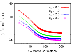
Figure 1: Time series of local density fluctuation $(\langle n(\sigma)^{2}\rangle-\langle n(\sigma)\rangle^{2})/\langle n(\sigma)\rangle$ for $\sigma=12$. Data are for $n_{c}=256$ NRRW chains of $N=512$ monomers in a box of size $L^{3}=128^{3}$. Several bending energies $\varepsilon_{b}$ are chosen, as indicated.

In Fig. 1 we show the typical time series of the local density fluctuation $(\langle n(\sigma)^{2}\rangle-\langle n(\sigma)\rangle^{2})/\langle n(\sigma)\rangle$ with $\sigma=12$ for $n_{c}=256$ NRRW chains of $N=512$ monomers in a box of size $L^{3}=128^{3}$, and for the bending energies $\varepsilon_{b}=0$ (fully flexible), $1.0$, $2.0$, and $3.0$. In the pre-packing process, the radius $\sigma$ is first set to $12\approx 4\ell_{b}$ in the unit of lattice spacings until all curves describing the local density fluctuation reach a plateau, and then reduced to $6\approx 2\ell_{b}$ until all curves reach another plateau again. The estimates of the collective structure factor $S(q)$ for $q=2\pi/L$ and the local density fluctuation $(\langle n(\sigma)^{2}\rangle-\langle n(\sigma)\rangle^{2})/\langle n(\sigma)\rangle$ for $\sigma=12$ are of the same order of magnitude (see Sec. III.4) from the final configurations generated by this two-step pre-packing process. Each Monte Carlo step contains $n_{c}$ translation moves and $n_{c}$ pivot-like moves such that the locations of all chains in the box are rearranged by the trial moves. Each curve shown in Fig. 1 represents the results averaged over $32$ independent realizations. We see that the local density fluctuation can be reduced by about an order of magnitude after about $1000$ Monte Carlo steps.

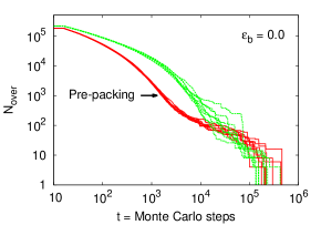
(a)      (b)

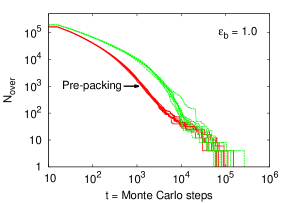
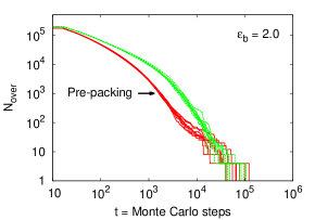
(c)      (d)

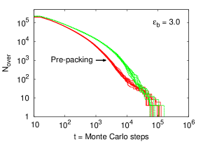
Figure 2: Time series of the total number of overlapping monomers $N_{\rm over}$ for polymer melts consisting of $n_{c}=256$ chains of $N=512$ monomers, and for $\varepsilon_{b}=0.0$ (a), $1.0$ (b), $2.0$ (c), and $3.0$ (d). Two sets of data for the simulations with (solid curves in red color online) and without (dashed curves in green color online) the pre-packing process, as indicated.

It is interesting to know what we have gained by introducing the pre-packing procedure before equilibrating the system. Therefore, we check the process of pushing away the monomers occupying the same unit cells (eight lattice sites are occupied by one effective monomer in BFM) by observing the time series of the number of overlapping monomers, $N_{\rm over}$, as the excluded volume effect is switched on. For simplicity, if a lattice site is occupied by $s$ effective monomers, it contributes $s-1$ overlapping monomers to $N_{\rm over}$. The transition process from $n_{c}=256$ NRRW chains of $N=512$ monomers to SAW chains is observed according to the decrease of $N_{\rm over}$ shown in Fig. 2 for $\varepsilon_{b}=0.0$, $1.0$, $2.0$, and $3.0$. Two sets of data ($8$ samples for each) representing the push-off process before (dashed curve in green color online) and after (solid curves in red color online) the pre-packing process is applied. Here one MC step is a sequence of $N_{\rm tot}$ L26 moves, and $Nn_{c}$ slithering-snake moves. In the slithering-snake moves, an end-monomer of each chain is selected and attempted to move once until all chains have been chosen, and then the same procedure is repeated $N$ times. A trial move is accepted if $\Delta N_{\rm over}=N_{\rm over}^{\rm(new)}-N_{\rm over}^{\rm(old)}<0$ and $\exp(-\Delta U_{b})/k_{B}T>r$ where $r$ is a random number and $r\in[0,1)$. The latter condition is the Metropolis criterion preserving the stiffness of the chains. If only L26 moves are applied in this push-off process, at the beginning it is very efficient to push off overlapping monomers, but then some chains are trapped in a state containing knots, or a state blocked by other chains. The slithering-snake moves therefore indeed play an important role at the intermediate stages for the chains escaping from a trapped state. From our observations in Fig. 2 it seems that applying an additional pre-packing process does not speed up the push-off process. However, it is still necessary to investigate the conformation of chains in a melt carefully.

In addition, it is interesting to note that pre-packing leads to a significantly faster decrease of $N_{\rm over}$ with time during intermediate stages of the process. This feature may be of interest in cases where one does not require that strictly $N_{\rm over}=0$ in the initial stage of the averaging. Consider e.g. a variant of the model where monomers overlap is not strictly forbidden (which corresponds to an infinitely high repulsive energy) but only leads to a large but finite energy penalty, e.g. $E_{\rm over}=20k_{B}T$. The probability to accept a move which increases the overlap then is of order $10^{-9}$, i.e. essentially negligible, and for long chains the statistical properties of the model are essentially the same as for the model with strict excluded volume. For such a model the overlap energy per monomer reduces after about $10^{4}$ Monte Carlo steps from an initial value (of the order of $20k_{B}T$) by three orders of magnitude, i.e. $0.02k_{B}T$, and this small number is reached $3$ to $4$ times faster with pre-packing than without it. For very large systems (and complicated models, leading to slow simulation algorithms) it may hence be an acceptable compromise to allow a small fraction ($10^{-3}$ or less) of overlap in the system.

In Table 1 we compare the average values of local density fluctuation $(\langle n(\sigma)^{2}\rangle-\langle n(\sigma)\rangle^{2})/\langle n(\sigma)\rangle$ {Eq. (II)} for $\sigma=12$ (since $q_{\rm min}=2\pi/L\approx V_{\rm sub}^{-1/3}$) over $32$ configures at different stages from the preparation of the initial configurations to the final configurations at the equilibrium state. Two ways of preparing the initial configurations (Sec. II) are compared as follows: (1) Randomly generating weakly-interactive NRRWs (NRRWs), applying the pre-packing process (Pre-packing, NRRWs), and switching on the excluded volume effect (Pre-packing+EV, SAWs). (2) Randomly generating weakly-interactive NRRWs (NRRWs) and switching on the excluded volume effect (EV, SAWs). We see that for weakly-interactive NRRWs the local density fluctuation decreases as the bending energy $\varepsilon_{b}$ increases. Since the bond angles tend to become smaller, the distance between non-bonded monomers apart from each other along the chain becomes longer. After the pre-packing process the fluctuation reduces by about $95\%$. Once the excluded volume interactions between monomers are switched on, the fluctuation remains almost the same for all cases.

Table 1: Values of local density fluctuation $(\langle n^{2}\rangle-\langle n\rangle^{2})/\langle n\rangle$ for $\sigma=12$. Data are for $N=512$, and for $\varepsilon_{b}=0.0$, $1.0$, $2.0$, $3.0$, averaged over 32 configurations at different stages.

$\varepsilon_{b}$	0.0	1.0	2.0	3.0
NRRWs	51.06	30.96	20.89	14.57
Pre-Packing, NRRWs	2.92	1.56	1.04	0.86
Pre-Packing+EV, SAWs	0.28	0.28	0.28	0.28
EV, SAWs	0.27	0.27	0.28	0.27
Equilibrium, SAWs	0.28	0.28	0.27	0.27

III.2 Mean square internal end-to-end distance and bond-bond orientational correlation function

For understanding the connectivity and correlation between monomers the conformations of linear chains of contour length $L=(N-1)\ell_{b}$ in a melt are normally described by the average mean square internal end-to-end distance, $\langle R^{2}(s)\rangle$,

$$\langle R^{2}(s)\rangle=\left\langle\frac{1}{n_{c}}\sum_{n=1}^{n_{c}}\left[\frac{1}{N-s}\sum_{j=1}^{N-s}(\vec{r}_{n,j}-\vec{r}_{n,j+s})^{2}\right]\right\rangle\,,$$ (4)

where $s$ is the chemical distance between the $j^{\rm th}$ monomer and the $(j+s)^{\rm th}$ monomer along the identical chain. The theoretical prediction of the internal mean square end-to-end distance for polymer melts consisting of semiflexible chains in the absence of excluded volume effect described by a freely rotating chain model is Flory1969

$$\langle R^{2}(s)\rangle=s\ell_{b}^{2}\left[\frac{1+\langle\cos\theta\rangle}{1-\langle\cos\theta\rangle}-\frac{2\langle\cos\theta\rangle(1-(\langle\cos\theta\rangle)^{s}}{s(1-\langle\cos\theta\rangle)^{2}}\right]\,,$$ (5)

with

$$\ell_{b}^{2}=\langle\vec{b}^{2}\rangle\qquad{\rm and}\qquad\langle\cos\theta\rangle=\langle\vec{b}_{i}\cdot\vec{b}_{i+1}\rangle/\ell_{b}^{2}$$ (6)

where $\ell_{b}$ is the root-mean-square bond length. In the limit $N\rightarrow\infty$, the bond-bond orientational correlation function in the absence of excluded volume effects therefore decays exponentially as a function of chemical distance $s$ between any two bonds along a linear chain Grosberg1994 ; Rubinstein2003 ,

$$\langle\vec{b}_{i}\cdot\vec{b}_{i+s}\rangle=\ell_{b}^{2}\langle\cos\theta(s)\rangle=\ell_{b}^{2}\langle\cos\theta\rangle^{s}=\ell_{b}^{2}\exp(-s\ell_{b}/\ell_{p})\,,$$ (7)

where $\ell_{p}$ is the so-called persistence length which can be extracted from the initial decay of $\langle\cos\theta(s)\rangle$. Equivalently, one can calculate the persistence length from

$$\ell_{p,\theta}/\ell_{b}=-1/\ln(\langle\cos\theta\rangle)$$ (8)

here instead of $\ell_{p}$ we use $\ell_{p,\theta}$ to distinguish between these two measurements. Replacing $s$ by $N-1$ in Eq. (5) it gives the asymptotic behavior of the mean square end-to-end distance of a FRC equivalent to the behavior of a freely jointed chain

$$\langle R_{e}^{2}\rangle = C_{\infty}(N-1)\ell_{b}^{2}\quad{\rm with}\quad C_{\infty}=\frac{1+\langle\cos\theta\rangle}{1-\langle\cos\theta\rangle}$$ (9)

$$= n_{K}\ell_{K}^{2}=2\ell_{p}L$$ (10)

where $C_{\infty}$ is called Flory’s characteristic ratio Flory1969 , $\ell_{K}=2\ell_{p}$ is the Kuhn length, and $n_{K}$ is the number of Kuhn segments.

We compare the estimates of $\langle R^{2}(s)\rangle$ obtained from the initial configurations of SAW chains generated by pushing off monomers occupying the same unit cell before and after the pre-packing process to that from those configurations in equilibrium as shown in Fig. 3. The two ways of preparing the initial configurations with and without the pre-packing process are denoted by “EV” and “Pre-packing+EV”, respectively in the figure. Results are obtained by taking the average over $32$ initial configurations of SAW chains for each case. We see that there is only a slight discrepancy in the estimates of $\langle R^{2}(s)\rangle$ obtained from the initial configurations and from the equilibrated configurations. The discrepancy becomes more prominent for $\varepsilon_{b}=3.0$. We see that there is no significant advantage of preparing the initial configurations of lattice chains in a melt through the pre-packing process as that was observed for the continuum chains.

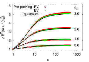
Figure 3: Rescaled internal mean square end-to-end distance, $\langle R^{2}(s)\rangle/(s\ell_{b}^{2})$, plotted as a function of $s$ for polymer melts containing $n_{c}=256$ chains of $N=512$ monomers, and for $\varepsilon_{b}=0.0$, $1.0$, $2.0$, and $3.0$. Data are for the estimates obtained from the initial configurations of SAWs generated by the two methods, ”Pre-packing+EV”, and ”EV”, and from the equilibrated configurations.

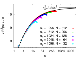
(a)      (b)

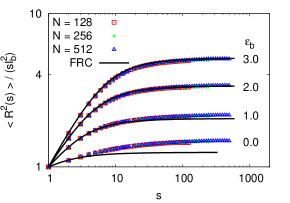
Figure 4: (a) $\langle R^{2}(s)\rangle/s$ plotted versus $s$ for polymer melts consisting of $n_{c}N=131072$ monomers, and for $\varepsilon_{b}=0.0$. (b) $\langle R^{2}(s)\rangle/(s\ell_{b}^{2})$ plotted versus $s$ for polymer melts of $N=128$, $256$ and $512$ monomers, and for various values of bending energy $\varepsilon_{b}$, as indicated. The theoretical predictions, Eq (11) with $b_{e}=3.244$ and $c_{s}=0.412$ in (a), and Eq. (5) in (b), are shown by curves for comparison.

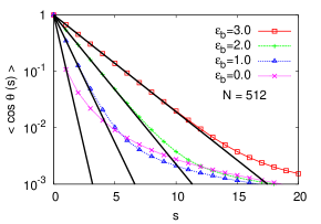
(a)      (b)

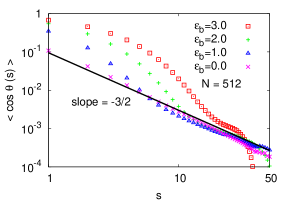
Figure 5: (a) Semi-log plot of the bond-bond orientational correlation function $\langle\cos\theta(s)\rangle$ vs. $s$. (b) Same data as shown in (a), but on a log-log scale. Data are for polymer melts consisting of semiflexible chains of size $N=512$, and for $\varepsilon_{b}=0.0$, $1.0$, $2.0$ and $3.0$, as indicated. In (a) the straight lines indicate the fits of the initial decay, $\langle\cos\theta(s)\rangle\propto\exp(-s\ell_{b}/\ell_{p})$ (Eq. (7)), for $\varepsilon_{b}>0$. For $\varepsilon_{b}=0$ the straight line is described by $\exp(-s\ell_{b}/\ell_{p,\theta})$. Values of $\ell_{p}/\ell_{b}$ and $\ell_{p,\theta}/\ell_{b}$ are listed in Table III. In (b) the straight line indicates the power law, $\langle\cos\theta(s)\rangle\propto s^{-3/2}$.

Table 2: Estimates of root-mean-square end-to-end distance $\langle R_{e}^{2}\rangle^{1/2}$, gyration radius $\langle R_{g}^{2}\rangle^{1/2}$, and bond length $\ell_{b}=\langle\vec{b}^{2}\rangle^{1/2}$ for polymer melts containing $n_{c}$ fully flexible chains of $N$ monomers ($\varepsilon_{b}=0$).

$N$	$n_{c}$	$\langle R_{e}^{2}\rangle^{1/2}$	$\sqrt{6}\langle R_{g}^{2}\rangle^{1/2}$	$\ell_{b}$
32	4096	17.07	17.13	2.63
64	2048	24.74	24.75	2.63
128	1024	35.54	35.51	2.63
256	512	50.76	50.73	2.63
512	256	72.17	72.20	2.63

In the equilibration process, each Monte Carlo step contains $n_{c}N$ L26 moves where each monomer is selected once to move, $n_{c}$ slithering-snake moves where each chain is selected once to move, and $n_{c}$ pivot moves where each chain is also selected once to move. There are about $10^{6}$ independent configurations for each measurement in equilibrium. Figure 4 represents the well-equilibrated data for polymer melts in a box of size $L^{3}=128^{3}$. Results for fully flexible chains of chain sizes $N=32$, $64$, $128$, and $512$ shown in Fig. 4a are in perfect agreement with the theoretical prediction given in Ref. Wittmer2007 ; Wittmer2011 ,

$$R^{2}(s)=b_{e}^{2}s(1-c_{s}/\sqrt{s})\qquad{\rm for}\,1\ll s\ll N$$ (11)

where $b_{e}=\lim_{s\rightarrow\infty}(R^{2}(s)/s)^{1/2}$ is the “effective bond length” (which is different from the root-mean-square bond length $\ell_{b}$ between monomers along a chain), and $c_{s}\equiv\sqrt{24/\pi^{3}}/(\rho b_{e}^{3})$. Results for polymer melts of $N=128$, $256$, and $512$ monomers are shown in Fig. 4b for $\varepsilon_{b}=0.0$, $1.0$, $2.0$, and $3.0$. The theoretical prediction for a freely rotating chain (FRC), Eq. (5), is also included for comparison. For $\varepsilon_{b}=0.0$ we see a strong deviation from the theoretical prediction since chains tend to swell due to the excluded volume effect that causes the $1/\sqrt{s}$ correction in Eq. (11). This is different from the results Auhl2003 ; Moreira2014 obtained using the bead-spring model in the continuum, where on short and intermediate length scales Eq. (5) for a FRC overestimates the internal distances for fully flexible chains, while on a large length scale it gives the accurate prediction. As the bending energy $\varepsilon_{b}$ increases, we see in Fig. 4b that the deviation from the prediction for a FRC reduces.

We also estimate the root-mean-square bond length $\ell_{b}=\langle\vec{b}^{2}\rangle^{1/2}$, end-to-end distance $\langle R_{e}^{2}\rangle$, and radius of gyration $\langle R_{g}^{2}\rangle$. Results for various values of $\varepsilon_{b}$ and $N$ are listed in Table 2 and 3. We see that $\langle R_{e}^{2}\rangle/\langle R_{g}^{2}\rangle\approx 6$ which is predicted for ideal chains. Our results of $\langle R_{e}^{2}\rangle$, $\langle R_{g}^{2}\rangle$, and $\ell_{b}$ for $\varepsilon_{b}=0.0$ and for various values of $N$ are in perfect agreement with the results given in Ref. Wittmer2007 although the total number of monomers of polymer chains in a melt and the lattice size which we have chosen for our simulations both are eight times smaller. The persistence lengths for polymer melts consisting of semiflexible chains determined by fitting the exponential decay, Eq. (7), and the correlation between two neighboring bonds, Eq. (8), are shown in Fig. 5a and also listed in Table 3 including Flory’s characteristic ratio $C_{\infty}$ using Eq. (9). Note that the asymptotic decay of $\langle\cos\theta(s)\rangle$ with $s$ is not exponential as predicted by Eq. (7), but rather a power law decay, $\langle\cos\theta(s)\rangle\propto s^{-3/2}$ for $s^{*}<s\ll N$, is expected, due to excluded volume effects Wittmer2007 ; Hsu2010 .

Therefore only the initial decay of $\langle\cos\theta(s)\rangle$ with $s$ ($s\ll s^{*}$) is meaningful for the estimation of the persistence length. In Fig. 5b we plot $\langle\cos\theta(s)\rangle$ versus $s$ on a log-log scale. The power law $s^{-3/2}$ is also shown for comparison. We see that the range over which the power law behavior holds ($s>s^{*}$) shrinks with increasing chain stiffness, and the data deviate from the straight line showing that the finite-size effect sets in. Results for various values of $\varepsilon_{b}$ and for chain sizes $N=128$ and $N=512$ are listed in Table 3. The relationship $\ell_{p}/\ell_{b}\approx\ell_{p,\theta}/\ell_{b}\approx C_{\infty}/2$ holds for semiflexible chains ($\varepsilon_{b}>0$) as predicted in Eqs. (9) and (10). The root-mean-square bond length $\ell_{b}\approx 2.63$ for polymer melts, shown in Table 2, is smaller than $\ell_{b}\approx 2.72$ for linear flexible chains in dilute solution based on the BFM. The reason is that the crowded environment of polymer chains prevents the bond vector between two effective monomers going through several unit cells, i.e. occupying large volume. We also see that $\ell_{b}$ depends only weakly on the stiffness of the chains as shown in Table 3.

Table 3: Estimates of root-mean-square end-to-end distance $\langle R_{e}^{2}\rangle^{1/2}$, gyration radius $\langle R_{g}^{2}\rangle^{1/2}$, bond length $\ell_{b}=\langle\vec{b}^{2}\rangle^{1/2}$, persistence lengths, $\ell_{p}/\ell_{b}$ and $\ell_{p,\theta}/\ell_{b}$, using Eqs. (7) and  (8), respectively, Flory’s characteristic ratio from Eq. (9), and the dimensionless compressibility $C_{g}=\rho k_{B}T\kappa_{T}$ from Eq. (27) for semiflexible chains in a melt for various values of bending energy $\varepsilon_{b}$, and for $N=512$ and $N=128$.

$N$	512				128
$\varepsilon_{b}$	0.0	1.0	2.0	3.0	0.0	1.0	2.0	3.0
$\langle R_{e}^{2}\rangle^{1/2}$	72.17	87.25	108.95	132.82	35.54	42.96	53.59	65.38
$\sqrt{6}\langle R_{g}^{2}\rangle^{1/2}$	72.20	87.12	108.69	132.48	35.51	42.84	53.20	64.41
$\ell_{b}$	2.63	2.62	2.62	2.61	2.63	2.62	2.62	2.61
$\ell_{p}/\ell_{b}$	_	0.96	1.64	2.53	_	0.96	1.64	2.53
$\ell_{p,\theta}/\ell_{b}$	0.45	0.95	1.64	2.53	0.45	0.95	1.64	2.53
$C_{\infty}$	1.24	2.06	3.38	5.12	1.24	2.06	3.38	5.12
$C_{g}$	0.25	0.24	0.23	0.23	0.25	0.24	0.23	0.23

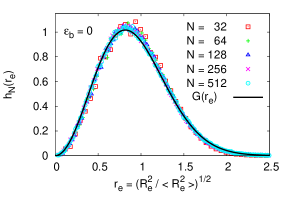
(a)      (b)

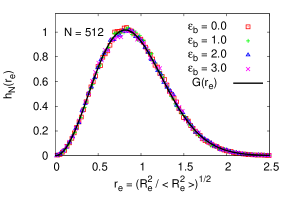
Figure 6: Normalized probability distributions of $r_{e}=(R_{e}^{2}/\langle R_{e}^{2}\rangle)^{1/2}$, $h_{N}(r_{e})$, plotted versus $r_{e}$ for polymer chains in a melt. In (a) data are for $\varepsilon=0.0$, and for various values of $N$, as indicated. In (b) data are for $N=512$, and for various values of $\varepsilon_{b}$, as indicated. The theoretical prediction $G(r_{e})$, {Eq. (17)}, (solid curve) is also shown for comparison.

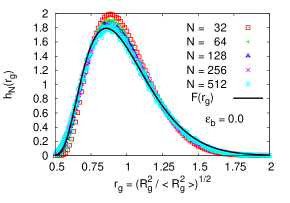
(a)      (b)

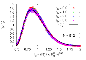
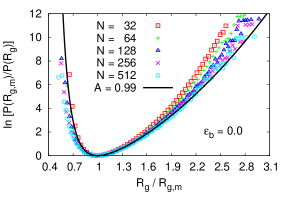
(c)      (d)

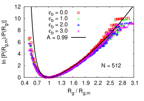
Figure 7: (a)(b) Normalized probability distributions of $r_{g}=(R_{g}^{2}/\langle R_{g}^{2}\rangle)^{1/2}$, $h_{N}(r_{g})$, plotted versus $r_{g}$ for polymer chains in a melt. (c)(d) Logarithm of the rescaled probability distribution of gyration radius, $\ln(P(R_{g,m})/P(R_{g}))$ as a function of $R_{g}/R_{g,m}$. In (a)(c) data are for $\varepsilon_{b}=0.0$, and for various values of $N$, as indicated. The theoretical prediction $F(r_{g})$, Eq. (18), (solid curve) is also shown for comparison. In (b)(d) data are for $N=512$, and for various values of $\varepsilon_{b}$, as indicated. The theoretical prediction $F(r_{g})$, Eq. (19), with $A=0.99$ (solid curve) is also shown for comparison.

III.3 Probability distributions of $R_{e}$ and $R_{g}$

The conformational behavior of polymer chains of size $N$ in a melt can also be described by the probability distributions of end-to-end distance $\vec{R}_{e}$ and gyration radius $R_{g}$, $P_{N}(\vec{R}_{e})$ and $P_{N}(R_{g})$, respectively. The probability distribution of $\vec{R}_{e}$ for ideal chains is simply a Gaussian distribution,

$$P_{N}(\vec{R}_{e})=\left(\frac{3}{2\pi N\ell_{b}^{2}}\right)^{3/2}\exp\left(-\frac{3R_{e}^{2}}{2N\ell_{b}^{2}}\right)\,.$$ (12)

There exists exact theoretical prediction of the probability distribution of $R_{g}$ for ideal chains Yamakawa1970 ; Fujita1970 ; Denton2002 , but they are complicated to evaluate. However, it has been checked Vettorel2010 ; Hsu2014 ; Froehlich2013 that the same formula suggested by Lhuillier Lhuillier1988 for polymer chains under good solvent conditions in $d$-dimensions is still a good approximation for ideal chains, i.e.,

$$P_{N}(R_{g})\sim\exp\left[-a_{1}\left(\frac{N^{\nu}}{R_{g}}\right)^{\alpha d}-a_{2}\left(\frac{R_{g}}{N^{\nu}}\right)^{\delta}\right]$$ (13)

where $a_{1}$ and $a_{2}$ are (non-universal) constants, and the exponents $\alpha$ and $\delta$ are linked to the space dimension $d$ and the Flory exponent $\nu$ by $\alpha=(\nu d-1)^{-1}$ and $\delta=(1-\nu)^{-1}$. Here $(1+\alpha)$ is the des Cloizeaux exponent Cloizeaux1975 for the osmotic pressure of a semidilute polymer solution, and $\delta$ is the Fisher exponent Fisher1966 characterizing the end-to-end distance distribution.

Numerically, the probability distribution of $x$ is obtained by accumulating the histogram $H_{N}(x)$ of $x$ over all configurations and all chains of size $N$, given by

$$H_{N}(x)=\sum_{\rm config.}\delta_{x,x^{\prime}}$$ (14)

here $x$ stands for $R_{e}$ or $R_{g}$. Note that an angular average over all directions has been included in the accumulating process of the histogram due to spherical symmetry. Thus, the normalized histogram of $x$ is given by

$$h_{N}(x)=H_{N}(x)/\sum_{x^{\prime}}H_{N}(x^{\prime})=4\pi C_{N}x^{2}P_{N}(x)$$ (15)

where $C_{N}$ is the normalization factor such that

$$C_{N}\int_{0}^{\infty}4\pi x^{2}P_{N}(x)=1\,.$$ (16)

In order to compare the probability distributions of $R_{e}$ and $R_{g}$ between various different chain sizes $N$ and bending energies $\varepsilon_{b}$, instead of $R_{e}$ and $R_{g}$ we use the reduced end-to-end distance $r_{e}=(R_{e}^{2}/\langle R_{e}^{2}\rangle)^{1/2}$ and the reduced gyration radius $r_{g}=(R_{g}^{2}/\langle R_{g}\rangle)^{1/2}$. Results of the normalized histogram $h_{N}(r_{e})$ compared to the theoretical prediction

$$G(r_{e})=4\pi r_{e}^{2}C_{N}\left(\frac{3}{2\pi}\right)^{3/2}\exp\left(-\frac{3r_{e}^{2}}{2}\right)$$ (17)

using $\langle R_{e}^{2}\rangle\sim N$ and Eq. (12) are shown in Fig. 6. Here the normalization factor $C_{N}=1$ for all cases. We see the nice data collapse for chain sizes $N\geq 64$ and all bending energies $\varepsilon_{b}$ in Fig. 6a,b and the data are described by a universal scaling function $G(r_{e})$ for ideal chains. For $N=32$ the data deviates from the master curve due to the finite-size effect. Results of the normalized histogram $h_{N}(r_{g})$ compared to the theoretical prediction

$$F(r_{g})=4\pi r_{g}^{2}C_{N}\exp\left(-b_{1}r_{g}^{-\alpha d}-b_{2}r_{g}^{\delta}\right)$$ (18)

using $\langle R_{g}^{2}\rangle=k_{g}^{2}N$ where $k_{g}$ is a constant and Eq. (13) are shown in Fig. 7. Here the normalization factor $C_{N}$, parameters $b_{1}=a_{1}k_{g}^{-\alpha d}$ and $b_{2}=a_{2}k_{g}^{\delta}$ are determined numerically depending on the simulation data, and they depend slightly on the chain size $N$. As $N\rightarrow\infty$ they will tend to asymptotic values (not shown). Near the peak ($r_{g}\approx 0.85$), we see the finite-size effect is stronger for the distribution of $r_{g}$. The fitting curve $F(r_{g})$ with parameters $b_{1}=0.09$, $b_{2}=2.29$, and $C_{N}=1.31$ determined by the least-square fit for $N=512$ and $\varepsilon_{b}=0.0$ and $b_{1}=0.075$, $b_{2}=2.20$, and $C_{N}=1.13$ for $N=512$ and $\varepsilon_{b}=3.0$ are shown in Fig. 7a,b, respectively for comparison. The distribution $P(R_{g})\propto H_{N}/R_{g}^{2}$ has its maximum value, i.e. $P(R_{g}=R_{g,m})=\max\;P(R_{g})$, and the corresponding gyration radius $R_{g,m}\propto R_{g}\propto N^{\nu}$. Therefore, using Eq. (13), the logarithm of the rescaled probability distribution as a function of $(R_{g}/R_{g,m})$ is given by

$$f\left(\frac{R_{g,m}}{R_{g}}\right)=\ln\frac{P(R_{g,m})}{P(R_{g})}$$ (19)

$$= A\left[\frac{1}{\alpha}\left(\frac{R_{g,m}}{R_{g}}\right)^{\alpha d}+\frac{d}{\delta}\left(\frac{R_{g}}{R_{g,m}}\right)^{\delta}+1-d\right]$$

with

$$a_{1}=\frac{A}{\alpha}\left(\frac{R_{g,m}}{\ell_{b}N^{\nu}}\right)^{\alpha d}\quad{\rm and}\quad a_{2}=\frac{Ad}{\delta}\left(\frac{\ell_{b}N^{\nu}}{R_{g,m}}\right)^{\delta}\,.$$ (20)

where one fitting parameter $A$ is left. Results of $\ln\{P(R_{g,m})/P(R_{g})\}$ plotted versus $R_{g}/R_{g,m}$ are presented in Fig. 7c,d. We see that due to the finite-size effect, data for fully flexible chains in a melt shown in Fig. 7c,d only start to converge for $N>128$. As $N$ increases, the systematical errors need to be taken into account. Using the least square fit, it gives $A=0.99(3)$. It is obvious that the distribution can only be well described by Eq. (19) for $R_{g}>R_{g,m}$, similar as that was found for Gaussian chains in Ref. Hsu2014 . For polymer melts of a fixed chain length $N=512$, we see that for $R_{g}<R_{g,m}$ the distribution remains the same for different stiffnesses, while for $R_{g}>R_{g,m}$ the data for $\varepsilon_{b}=0$ are slightly deviated from the data for $\varepsilon_{b}>0$. We plot the same distribution, Eq. (19) with $A=0.99$ for comparison.

III.4 Structure factor and compressibility

The collective static structure factor $S(q)$ of polymer melts is defined by the total scattering from the center of all monomers inside the box, regardless of whether they are linked along a polymer chain or not,

$$S(q)=\frac{1}{N_{\rm tot}}\left\langle\sum_{i=1}^{N_{\rm tot}}\sum_{j=1}^{N_{\rm tot}}\exp[i\vec{q}\cdot(\vec{r}_{i}-\vec{r}_{j})]\right\rangle\,.$$ (21)

Here $N_{\rm tot}=Nn_{c}$ are the total number of monomers and $\langle\cdots\rangle$ represents the average over all independent configurations, and over all vectors $\vec{q}$ of the same size $q=\mid\vec{q}\mid$. Note that since a simple cubic lattice of size $L^{3}$ with periodic boundary condition is considered for our simulations, only the following $\vec{q}$ are allowed,

$$\vec{q}=\frac{2\pi}{L}(n_{1},n_{2},n_{3})$$ (22)

where $n_{i}=0,\pm 1,\pm 2,\ldots$ for $i=1$, $2$, and $3$, and $q\geq 2\pi/L$. $S(q)$ characterizes a competition between the intramolecular fluctuations ($S_{\rm intra}$) and the intermolecular correlations ($S_{\rm inter}$), thus one can write

$$S(q)=S_{\rm intra}(q)+S_{\rm inter}(q)$$ (23)

with

$$S_{\rm intra}=\frac{1}{n_{c}}\left\langle\sum_{n=1}^{n_{c}}\frac{1}{N}\sum_{i,j=1}^{N}\exp[i\vec{q}\cdot(\vec{r}_{i}^{n}-\vec{r}_{j}^{n})]\right\rangle=S_{c}(q)$$ (24)

and

$$S_{\rm inter}=\frac{1}{N_{\rm tot}}\sum_{i,j=1}^{N}\left\langle\sum_{n=1,n\neq n^{\prime}}^{n_{c}}\sum_{n^{\prime}=1}^{n_{c}}\exp[i\vec{q}\cdot(\vec{r}_{i}^{n}-\vec{r}_{j}^{n^{\prime}})]\right\rangle$$ (25)

where the contributions from the intramolecular fluctuations are simply equivalent to the average of the standard static structure factor of single polymer chains in a melt, $S_{c}(q)$.

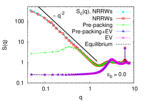
(a)      (b)

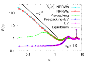
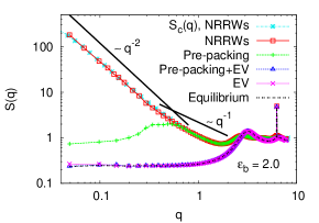
(c)      (d)

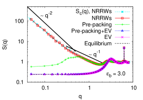
Figure 8: Structure factor $S(q)$ from the scattering of polymer melts plotted vs. $q$ on log-log scales for $\varepsilon_{b}=0.0$ (a), $1.0$ (b), $2.0$ (c) and $3.0$ (d). Results are for the conformations of polymer melts at different stages, initial NRRWs (NRRWs), rearranged NRRWs after applying pre-packing process (Pre-packing), SAWs obtained from NRRWs by the push-off process before applying the pre-packing procedure (EV), and after (Pre-packing+EV), and equilibrated SAWs after polymer melts reaching equilibrium (Equilibrium). The structure factor $S_{c}(q)$ for single NRRWs chains generated initially and the Scaling predictions for Gaussian coils, $S(q)\sim q^{-2}$, and for rigid rods, $S(q)\sim q^{-1}$, are also shown for comparison.

The collective structure factors $S(q)$ which represent the conformations of the whole polymer system at different stages from weakly-interactive NRRW chains to equilibrated SAW chains in a melt for $N=512$ and for $\varepsilon_{b}=0.0$, $1.0$, $2.0$, and $3.0$ are shown in Fig. 8. Results include the initial NRRW chains (NRRWs), rearranged NRRW chains through the pre-packing process (Pre-packing), initial SAW chains obtained from the initial NRRW chains by switching on the excluded volume effect before (EV) and after (Pre-packing+EV) applying the pre-packing procedure, and the equilibrated SAW chains in a melt (Equilibrium). Each curve shows the result averaged over $32$ independent configurations at the intermediate states, while $1500$ independent configurations are considered for the measurement in equilibrium. The average static structure factor of single NRRW chains generated initially, $S_{c}(q)$, is also included for comparison. In Fig. 8 we see that in all cases there is no interactions between NRRWs generated in the box at the beginning, so the structure factor shows the same scaling behavior for single NRRWs in dilute solution, i.e. $S(q)=S_{c}(q)$. The scaling predictions $S(q)\sim q^{-1/\nu_{id}}$ with $\nu_{id}=1/2$ for ideal chains and $S(q)\sim q^{-1}$ for rigid rods are verified for fully flexible and moderately stiff chains. After the pre-packing process where NRRW chains are rearranged, the collective structure factor decreases in the low-q regime. Once all overlapping monomers are pushed off there is no difference between the configurations generated by the push-off process with and without the pre-packing in the intermediate and large $q$, but for very small $q$ a small discrepancy exists between those data sets. It is consistent with our previous observation of $\langle R^{2}(s)\rangle$ in Fig. 3 that the discrepancy becomes more prominent at larger scales.

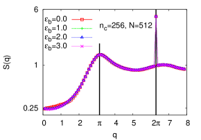
Figure 9: Structure factors $S(q)$ of polymer melts, plotted vs. $q$ on semi-log scales Data are for polymer melts consisting of $n_{c}=256$ chains of lengths $N=512$, and for various values of $\varepsilon_{b}$, as indicated. In (a) the peak appears at $q\approx\pi$ measuring the mean inter-particle distance in the polymer melts, and the second peak at $q\approx 2\pi$ is the so-called Bragg peak.

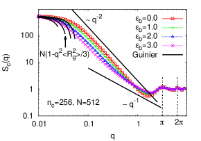
(a)      (b)

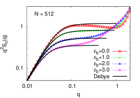
Figure 10: (a) Structure factors of single chains in a melt, $S_{c}(q)$, plotted vs. $q$ on log-log scales. (b) Same data as in (a) but in a Kratky-Plot. Data are for polymer melts consisting of $n_{c}=256$ chains of $N=512$ monomers, and for various values of $\varepsilon_{b}$, as indicated. In (a) the theoretical predictions $S_{c}(q)=N(1-q^{2}\langle R_{g}^{2}\rangle/3)$ at the Guinier regime for small $q$, $S_{c}(q)\sim q^{-2}$ for a Gaussian coil, and $S_{c}(q)\sim q^{-1}$ for a rigid rod are shown by solid curves for comparison. In (b) the Debye function, Eq. (26), is also shown for comparison.

In the following we only focus on polymer melts consisting of $n_{c}=256$ chains of $N=512$ monomers in equilibrium. Figure 9 shows the results for the scattering from polymer melts in equilibrium. Four different choices of the stiffness characterized by the bending energy $\varepsilon_{b}$ are included. At small $q$ there is a systematic dependence on $\varepsilon_{b}$, reflecting the (rather weak) dependence of the compressibility on $\varepsilon_{b}$. It is remarkable that the structure factor of large values of $q$ is completely independent of the chain stiffness. As $q$ increases, the first peak, the so-called amorphous halo for non-crystalline materials, appears at $q\approx\pi$ measuring the mean inter-particle distance ($\sim 2$ lattice spacings) in a polymer melt. The second peak, the so-called Bragg peak, appears at $q\approx 2\pi$ probing the structure on the scale of the monomers ($\sim 1$ lattice spacing). The scattering from single chains in a melt in equilibrium is shown in Fig. 10. In Fig. 10 one sees that $S_{c}(q)\approx N\exp(-q^{2}\langle R_{g}^{2}\rangle/3)\approx N(1-q^{2}\langle R_{g}^{2}\rangle/3)$ for small $q$ in the Guinier regime, then a cross-over occurs to the power law of Gaussian coils (ideal chains), $S(q)\sim q^{-1/\nu_{\rm id}}$ with $\nu_{\rm id}=1/2$. For moderately stiff chains one observes also a rigid-rod regime $S(q)\sim q^{-1}$. The two peaks at $q\approx\pi$ and $q\approx 2\pi$ show up in a similar way as that for the collective structure $S(q)$ in Fig. 9 and are due to the underlying lattice model. In order to clarify whether single chains in a melt behave as ideal chains we show the structure factors $S_{c}(q)$ in a Kratky-plot in Fig. 10(b). The Debye function deGennes1979 ; Cloizeaux1990 ; Schaefer1999 ; Higgins1994 describing the scattering from Gaussian chains,

$$S_{\rm Debye}(q)=2\frac{\eta-1+\exp(-\eta)}{\eta^{2}}\quad{\rm with}\quad\eta=q^{2}\langle R_{g}^{2}\rangle\,,$$ (26)

is also presented in Fig. 10b for comparison. For fully flexible chains ($\varepsilon_{b}=0.0$) in a melt we see the discrepancy between our simulation results and the Debye function at the intermediate values of $q$, which agrees with the previous finding Wittmer2007i that polymer chains in a melt are not random walks. While for $\varepsilon_{b}=0.0$ the deviation from ideality is clearly recognized due to the minimum in the Kratky-plot near $q=1$, for $\varepsilon_{b}\geq 1.0$ there occurs no minimum any longer (for $N=512$). While the deviations from Gaussian statistics are still obvious from $\langle\cos\theta(s)\rangle$, Fig. 5, they are not easy to extract from $S_{c}(q)$. For $\varepsilon_{b}=1.0$ we see the Kratky plateau over all intermediate regimes, while the regime decreases as $\varepsilon_{b}$ increases since the rigid-rod behavior takes over.

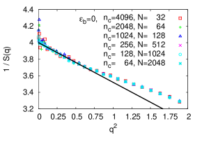
(a)      (b)

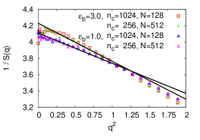
Figure 11: Inverse of structure factor of polymer melts, $1/S(q)$, plotted vs. $q^{2}$ for $\varepsilon_{b}=0.0$ (a), and $\varepsilon_{b}=1.0$, $3.0$ (b). Several chain lengths $(N-1)$ are chosen, as indicated. The asymptotic behavior of $1/S(q)$ as $q^{2}\approx 0$ is described by straight lines. Values of the dimensionless compressibility $C_{g}=\left[\lim_{q^{2}\rightarrow 0}1/S(q)\right]^{-1}$ are listed in Table 3.

The isothermal compressibility of $\kappa_{T}$ characterizing the degree of density fluctuations on large scale is a measure for the response of a systems volume to an increase in the system pressure Binder2011 ; Wittmer2011 , $\kappa_{T}\equiv-(1/V)(\partial V/\partial p)_{T}$, and is related to the structure factor $S(q)$ as $q\rightarrow 0$,

$$\lim_{q\rightarrow 0}S(q)=\rho k_{B}T\kappa_{T}=C_{g}$$ (27)

where $C_{g}$ is defined as the “dimensionless compressibility”. In Fig. 9 we see that as $q\rightarrow 0$ the estimates of the collective structure factor for polymer chains of size $N=512$ in a melt reach a plateau value $\lim_{q\rightarrow 0}S(q)\approx 0.25$. Due to the finite-size effect and lattice artifact ($q_{\rm min}=2\pi/L$), we take the same data but plot $1/S(q)$ versus $q^{2}$ in Fig. 11. We see the fluctuations of data near $q^{2}\rightarrow 0$. However, the best fit of the straight line going through our data gives the estimate of $C_{g}=\left[\lim_{q^{2}\rightarrow 0}1/S(q)\right]^{-1}$. Results are listed in Table 3. We see that $C_{g}\in[0.23,0.25]$ and depends only weakly on the stiffness of the chains.

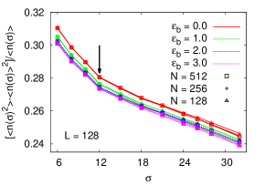
(a)      (b)

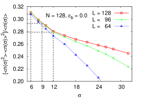
Figure 12: Local density fluctuations $\left[\langle n(\sigma)^{2}\rangle-\langle n(\sigma)\rangle^{2}\right]/\langle n(\sigma)\rangle$ plotted as a function of $\sigma$ for polymer chains of different stiffnesses in a melt (a) and for fully flexible chains of fixed chain length $N=128$ in a melt (b). Three values of chain length $N$ and four values of bending energy $\varepsilon_{b}$ are chosen, as indicated in (a). Three different sizes of lattice box are chosen, as indicated in (b). The locations of $\sigma=\sigma_{\rm min}=(4\pi/3)^{-1/3}(2\pi/L)^{-1}$ for various values of $L$ are indicated by an arrow in (a) and dashed lines in (b).

In the thermodynamic limit by taking the limit $N\rightarrow\infty$ (but keeping the density $\rho=N/V$ fixed), then taking the limit $q\rightarrow 0$, the local density fluctuations in subvolumina $V_{\rm sub}\ll V$ Baschnagel1994 ; Binder2011

$$\frac{\langle n(\sigma)^{2}\rangle-\langle n(\sigma)\rangle^{2}}{\langle n(\sigma)\rangle}=k_{B}T\rho\kappa_{T}=C_{g}$$ (28)

where $V_{\rm sub}=4\pi\sigma^{3}/3$. Choosing $\sigma=12$ such that $q_{\rm min}\approx V_{\rm sub}^{-1/3}$, i.e. in the limit $q\rightarrow q_{\rm min}=2\pi/L$, the local density fluctuations estimated from the configurations of polymer melts in equilibrium are listed in Table 1. The estimates of $C_{g}\in[0.27,0.28]$ are a little bit higher than the estimates from the collective structure factor, but they are compatible. We also check the finite-size effect on the estimate of the local density fluctuations. Fig. 12 shows the local density fluctuations $[\langle n(\sigma)^{2}\rangle-\langle n(\sigma)\rangle^{2}]/\langle n(\sigma)\rangle$ as a function of $\sigma$. The arrow and dashed lines shown in Fig. 12 indicate the estimate of the compressibility $c_{g}(L,\varepsilon_{b})$ at $\sigma=\sigma_{\rm min}\approx(4\pi/3)^{-1/3}(2\pi/L)^{-1}$. We see that the local density fluctuations at certain values of $\sigma$ ($\sigma<30$) do not depend on the chain lengths $N$ for chains of different stiffnesses, while the discrepancy between the data sets decreases as the stiffness of chains increases (see Fig. 12a). For $\sigma<\sigma_{\rm min}$ the local density fluctuations tend to diverge. As the size of polymer melts increases ($L$ increases, but $\rho=N/L^{3}$ is fixed) the curves toward to a flat curve for $\sigma>\sigma_{\rm min}$ (see Fig. 12b). According to the finite-size scaling the estimate of $c_{g}$ can be obtained by extrapolating the data of $c_{g}(L,\varepsilon_{b}$) to $L^{-1}\rightarrow 0$.

IV Conclusions

We have studied the conformations of polymer chains consisting of fully flexible and semiflexible chains in a melt based on the bond fluctuation model at volume fraction $\phi=0.5$. The initial configurations of polymer melts are prepared through several procedures. We first generate NRRWs in a box with periodic boundary conditions in all three directions, rearrange NRRWs by the pre-packing process to reduce the local density fluctuations or remain NRRWs at the same positions, and then push off overlapping monomers blocking the same lattice sites. We compare the conformations of polymer melts at the end of each process to the result obtained from the equilibrated configurations. Applying the additional pre-packing process seems to have no significant effect on preparing initial configurations of polymer chains in a melt based on the lattice model after the excluded volume interactions are switched on completely. Namely, the estimates of the mean square internal end-to-end distance $\langle R^{2}(s)\rangle$ and the collective structure factors $S(q)$ from the configurations generated by the two methods (denoted by Pre-packing+EV, and EV in Figs. 3 and  8) are almost the same, and very close to estimates from the equilibrated configurations. There is also no difference of the equilibrating time starting from the initial configurations generated by these two methods. If, however, one accepts a marginally incomplete elimination of excluded volume violations ($N_{\rm over}\approx 100$ for a system of $n_{c}N=131072$ monomers) one would have significant advantages. Another possibility of testing this pre-packing process for the future work would be to use it as a criterion of putting chains into the box at the beginning.

In our simulations we combine the algorithms of the local 26 moves, slithering-snake, and pivot moves (instead of double-bridging moves Wittmer2007 ; Wittmer2011 ) for equilibrating the system of polymer melts. Although the total number of monomers $N_{\rm tot}=131072$ which is eight times smaller than $N_{\rm tot}=1048576$ in Ref. Wittmer2007 based on the same model for $\varepsilon_{b}=0$, the estimates of the mean square end-to-end distance $\langle R_{e}^{2}\rangle$, the mean square gyration radius $\langle R_{g}^{2}\rangle$, the mean square bond lengths $\langle\vec{b}^{2}\rangle$, and the dimensionless compressibility $C_{g}$ are all in perfect agreement with those results given in Ref. Wittmer2007 at fixed chain size $N$. For fully flexible and moderately stiff chains the ratio $\langle R_{e}^{2}\rangle/\langle R_{g}^{2}\rangle\approx 6$ as expected for ideal chains. For moderately stiff chains in a melt the internal mean square end-to-end distance $\langle R^{2}(s)\rangle$ is well described by the freely rotating chain model. Results of the probability distributions of reduced end-to-end distance $r_{e}=(R_{e}^{2}/\langle R_{e}^{2}\rangle)^{1/2}$ and reduced gyration radius $r_{g}=(R_{g}^{2}/\langle R_{g}^{2}\rangle)^{1/2}$ for polymer chains in a melt for various values of $N$ and $\varepsilon_{b}$ show the nice data collapse, and are described by universal functions, Eqs. (17) and (18), for ideal chains. The collective structure factors $S(q)$ for the whole polymer melts and the standard structure factor $S_{c}(q)$ for single chains in a melt are also calculated and compared with the theoretical predictions. A detailed investigation of $S_{c}(q)$ in a Kratky-plot for $\varepsilon_{b}=0.0$, $1.0$, $2.0$, and $3.0$ shows that for fully flexible chains in a melt there is a significant deviation from the Debye function for Gaussian chains at the intermediate values of $q$ as found by Wittmer et al. Wittmer2007i , while for $\varepsilon_{b}=1.0$ it is perfectly described by the Debye function. Since real polymers (such as polystyrene) exhibit some local chain stiffness, it is clear that the deviations from Gaussian statistics found for fully flexible chains in melts in the Kratky-plot will be very difficult to test experimentally. However, since only chains up to $N=512$ are considered in our simulations, such a deviation may also occur as the chain length increases. Careful investigation of the structure factor and the mean square internal end-to-end distance for much longer semiflexible polymer chains in a melt will be required to clarify this matter. The dimensionless compressibility $C_{g}$ determined by the estimates of the collective structure factors $S(q)$ for small $q$ and the local density fluctuations $(\langle n^{2}\rangle-\langle n\rangle^{2})/\langle n\rangle$ within a sphere of radius $\sigma$ are compatible from our simulations for all cases. We hope that the present work will help to the further development of a coarse-graining approach by using the BFM as an underlying microscopic model and will be useful for the interpretation of corresponding experiments searching for excluded volume effect in the scattering function of polymers in melts.

V Acknowledgments

I am indebted to K. Binder and K. Kremer for stimulating discussions and for carefully reading the manuscript, and also thank L. Moreira and W. Paul for their helpful discussions. I thank the Max Planck Institute for Polymer Research for the hospitality while this research was carried out. I also thank the John von Neumann Institute for Computing (NIC Jülich) for a generous grant of computer time and the Rechenzentrum Garching (RZG), the supercomputer center of the Max Planck Society, for the use of their computers.

References

- (1) P. J. Flory, Statistical mechanics of chain molecules, Wiley press, New York (1979).
- (2) P. G. de Gennes, Scaling Concepts in polymer physics, Cornell University Press: Itharca, New York. (1979).
- (3) K. Binder (ed.), Monte Carlo and molecular dynamics simulations in polymer science, Oxford University Press, New York (1995).
- (4) M. Kotelyanskii and D. N. Theodorou (ed), Simulation methods for polymers, Marcel Dekker, New York (2004).
- (5) K. Binder and W. Paul, Macromolecules 41, 4537 (2008).
- (6) M. Murat and K. Kremer, J. Chem. Phys. 108, 4340 (1998).
- (7) F. Müller-Plathe, ChemPhysChem 3, 754 (2002).
- (8) V. A. Harmandaris, D. Reith, N. F. A. van der Vegt, and K. Kremer, Macromol. Chem. Phys. 208, 2109 (2007).
- (9) V. A. Harmandaris, N. P. Adhikari, N. F. A. van der Vegt, and K. Kremer, Macromolecules 39, 6708 (2006).
- (10) P. D. Gujrati and A. I. Leonov (Ed.), Modeling and simulations in polymers, Wiley (2010).
- (11) T. Vettorel, G. Besold, and K. Kremer, Soft Matter 6, 2282 (2010).
- (12) G. Zhang, K. Ch. Daoulas, and K. Kremer, Macromol. Chem. Phys. 214, 214 (2013).
- (13) G. Zhang, L. A. Moreira, T. Stuehn, K. Ch. Daoulas, and K. Kremer, ACS Macro Lett. 3 198, (2014).
- (14) I. Carmesin and K. Kremer, Macromolecules 21, 2819 (1988).
- (15) H.-P. Wittmann and K. Kremer, Comp. Phys. Commun. 61, 309 (1990).
- (16) H. P. Deutsch and K. Binder, J. Chem. Phys. 94 2294 (1991).
- (17) W. Paul, K. Binder, D. W. Heermann, and K. Kremer, J. Phys. II 1 37 (1991).
- (18) J. P. Wittmer, A. Cavallo, H. Xu, J. E. Zabel, P. Polińska, N. Schulmann, H. Meyer, J. Farago, A. Johner, S. P. Obukhov, and J. Baschnagel, J. Stat. Phys. 145, 1017 (2011).
- (19) H. Yamakawa, Modern theory of polymer solutions, Harper and Row, New York (1971).
- (20) J. P. Wittmer, P. Beckrich, A. Johner, A. N. Semenov, S. P. Obukhov, H. Mayer, and J. Baschnagel, EPL 77 56003 (2007).
- (21) R. Auhl, R. Everaers, G. S. Grest, K. Kremer, and S. J. Plimpton, J. Chem. Phys. 119, 12718 (2003).
- (22) L. A. Moreira, F. Müller, T. Stühn, and K, Kremer, unpublished (2014).
- (23) H.-P. Hsu, J. Chem. Phys., 141, 164903 (2014).
- (24) J. P. Wittmer, W. Paul, K. Binder, Macromolecules 25, 7211 (1992).
- (25) J. P. Wittmer, P. Beckrich, H. Mayer, A. Cavallo, A. Johner, and J. Baschnagel, J. Phys. Rev. E 76, 011803 (2007).
- (26) A. Yu. Grosberg, and A. R. Khokhlov, Statistical Physics of Macromolecules AIP Press, NY, (1994).
- (27) M. Rubinstein and R. H. Colby, Polymer Physics, Oxford University Press, Oxford, (2003).
- (28) H.-P. Hsu, W. Paul, and K. Binder, Macromolecules 43, 3094 (2010).
- (29) H. Yamakawa, Modern theory of polymer solutions, Clarendon, Oxford (1970).
- (30) H. Fujita and T. Norisuye, J. Chem. Phys. 52, 1115 (1970).
- (31) A. R. Denton and M. Schmidt, J. Phys.: Condens. Matter 14, 12051 (2002).
- (32) M. G. Fröhlich and T. D. Sewell, Macromol. Theory Simul. 22, 344 (2013).
- (33) D. Lhuillier, J. Phys. France 49, 705 (1988).
- (34) J. des Cloizeaux, J. Phys. France 36, 281 (1975).
- (35) M. E. Fisher, J. Chem. Phys. 44, 616 (1966).
- (36) J. Des Cloizeaux and G. Jannink, Polymers in Solution: Their Modeling and Structure, Clarendon, Oxford (1990).
- (37) L. Schäfer, Excluded Volume Effects in Polymer Solutions as Explained by the Renormalization Group, Springer, Berlin, (1999).
- (38) J. S. Higgins and H. C. Benoit, Polymers and Neutron Scattering, Clarendon, Oxford (1994).
- (39) J. Baschnagel and K. Binder, Physica A 204, 47 (1994).
- (40) K. Binder and W. Kob, Glassy materials and disordered solids:An introduction to their statistical mechanis, 2nd ed., World Scientific press, Singapore (2011).