Engineering the initial state in broadband population inversion

Abstract

Quantum systems with sublevel structures prevent full population inversion from one manifold of sublevels to the other using strong ultrafast resonant pulses. In this work we explain the mechanism by which this population transfer is blocked. We then develop a novel concept of geometric control, assuming full or partial coherent manipulation within the manifolds and show that by preparing specific coherent superpositions in the initial manifold, full population inversion or full population blockade, i.e laser-induced transparency, can be achieved. In particular, by parallel population transfer we show how population inversion between the manifolds can be obtained with minimal pulse area. As the number of sublevels increases, population inversion can overcome the pulse area theorem at the expense of full control over the initial manifold of sublevels.

In this work we are concerned with intrinsic properties of the dynamics of systems with manifolds of sublevels, described by two (or more) quantum numbers, that hereafter will be generically called quantum structures. From the point of view of controlling the system dynamics, quantum structures pose several interesting problems. Quantum controlQC typically implies the ability to manipulate interfering pathways, which increases with the number of levels that participate in the dynamics as long as the system is controllable controllability . A multi-level structure would therefore offer more control opportunities at the expense of the ability to manipulate within the substructures. Our general goal is to investigate whether quantum structures limit, or conversely help, in controlling the system. In this paper we will be concerned with coarse-grained goals, where the objective of the control will be the state of the manifold given by the first quantum number, not the detailed state of the sublevels. In finding the best possible controls we will assume that the substructure is partially controllable, that is, that given some constraints, any possible wave function within a subset of the sublevels can be prepared wfcontrol . Building on this assumption we will develop a geometric control approach that allows finding the optimal initial wave functions that maximize the yield of the desired process. This procedure does not prescribe an optimal field, but implicitly assumes that a field can be found, and makes full use of the quantum structures.

Let us consider a simple and very general process in systems with a congested spectrum: absorption from the ground, initial manifold to the excited, target manifold, by means of a strong ultrashort pulse, with a bandwidth much larger than the energy spacing of the sublevels within the fine structure. As a molecular example, we can conceive controlling an electronic transition using a broadband pulse, where the goal is to invert the population to the excited state, regardless of the vibrational populationsmolpipulse . Although one may think that the substructure, specially in the case of very different associated time-scales, does not affect the overall transition, in the strong field case the opposite occurs. The unpopulated levels of the fine structure induce Stark shiftsStarkshift and create effective detunings from the resonance that limit the extent of the Rabi oscillations. That is, assuming that all the different sublevels are dipole allowed, regardless of the strength of the pulse, the maximum population that can be reached is typically much smaller than one.

A simple theoretical model explains this observation. Let us first assume that the different sublevels within each manifold are degenerate, $\Delta E\ll\Delta\omega\approx 0$, and that all transient dipoles are equal. Then the equations of motion for every sublevel of the excited manifold $|e,k\rangle$, and for every sublevel in the initial manifold $|g,j\rangle$, are the same. For a resonant transition: $\dot{a}_{j}=i\Omega(t)\sum_{k}b_{k}(t)/2$ and $\dot{b}_{n}=i\Omega(t)\sum_{j}a_{j}(t)/2$, where $\Omega(t)$ is the Rabi frequency. However, the initial conditions in the manifold $|g,j\rangle$, where we assume a single state, $|g,1\rangle$, is initially populated, break the symmetry so that three different probability amplitudes describe the dynamics. We write,

$$|\Psi(t)\rangle=a(t)|g,1\rangle+\bar{b}(t)\sum_{k}^{N_{f}}|e,k\rangle+\bar{c}(t)\sum_{j^{\prime}}^{N_{i}-1}|g,j^{\prime}\rangle$$ (1)

where the prime indicates that the initial state is excluded from the summation in the $|i,j\rangle$ manifold, and $\bar{b}(t)$ and $\bar{c}(t)$ are mean probability amplitudes, which in fact behave exactly as every sublevel amplitude. We define now the collective excited $|E\rangle$ and Raman $|R\rangle$ states

$$|E\rangle=\frac{1}{\sqrt{N_{f}}}\sum_{k}^{N_{f}}|e,k\rangle$$ (2)

$$|R\rangle=\frac{1}{\sqrt{N_{i}-1}}\sum_{j^{\prime}}^{N_{i}-1}|g,j^{\prime}\rangle$$ (3)

which together with the initial state $|i\rangle\equiv|g,1\rangle$ form an orthonormal basis such that $|\Psi(t)\rangle=a(t)|i\rangle+B(t)|E\rangle+C(t)|R\rangle$ with $B(t)=\sqrt{N_{f}}\,\bar{b}(t)$, $C(t)=\sqrt{N_{i}-1}\bar{c}(t)$, and $|a(t)|^{2}+|B(t)|^{2}+|C(t)|^{2}=1$. The effective Hamiltonian in this basis is

$${\sf H}:=-\frac{1}{2}\sqrt{N_{f}}\Omega(t)\left(|i\rangle\langle E|+\sqrt{N_{i}-1}|E\rangle\langle R|+\mathrm{c.c.}\right)$$ (4)

with simple analytic eigenvalues and eigenvectors (aka dressed states) Shore . When $N_{i}=2$ the wave function dynamics is particularly interesting, with a population in the manifold of excited states given by

$$P_{E}(t)=\sum_{k}^{N_{f}}|\langle e,k|\Psi(t)\rangle|^{2}=|\langle E|\Psi(t)\rangle|^{2}=\frac{1}{2}\sin^{2}\left(\sqrt{\frac{N_{f}}{2}}\theta(t)\right)$$ (5)

where $\theta(t)=\int_{-\infty}^{t}\Omega(t^{\prime})dt^{\prime}$, such that $\theta(\infty)$ is the pulse area, ${\cal A}$. A maximum of $50$% population can reach the excited state, whereas there is Rabi flopping (at twice the period of oscillation) between the initial state $|i\rangle$ ($|i,1\rangle$) and $|R\rangle$ ($|i,2\rangle$),

$$P_{R}(t)=|\langle R|\Psi(t)\rangle|^{2}=\sin^{4}\left(\frac{1}{2}\sqrt{\frac{N_{f}}{2}}\theta(t)\right)$$ (6)

i.e. there is a very efficient Raman Stokes transition. Increasing the number of sublevels in the initial manifold only blocks the population transfer more efficiently. For large $N_{i}$, we obtain a population in the excited manifold of

$$P_{E}(t)=\frac{1}{N_{i}}\sin^{2}\left(\frac{1}{2}\sqrt{N_{f}N_{i}}\theta(t)\right)$$ (7)

Unlike in $N_{i}=2$, for large $N_{i}$ the maximum Raman populations depend also on $N_{i}^{-1}$. Larger pulse areas only increase the frequency of the oscillations, but the initial state is mostly decoupled. The population dynamics behave as in an off-resonant excitation, with an effective detuning created by the Autler-Townes splittingAutlerTownes between the $|E\rangle$ and $|R\rangle$ states, coupled by an $\sqrt{N_{i}-1}$ stronger Rabi frequency than the initial state with the $|E\rangle$ state.

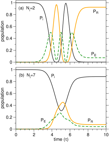
Figure 1: Population histories for a system with (a) $N_{i}=2$ ($N_{f}=1$), (b) $N_{i}=7$ ($N_{f}=7$). In both cases the pulse area is ${\cal A}=5\pi$ and the energy difference between the levels is $\Delta E=0.4\tau^{-1}$.

Fig.1 shows the population dynamics for different sublevel structures, using time-scaled units. Case 1 refers to $N_{i}=2$, $\Delta E=0.4\tau^{-1}<\Delta\omega=4\ln{2}$ (where $\Delta\omega$ is the bandwidth of the Gaussian pulse, with scaled width, $\tau=1$), $N_{f}=1$ and the peak Rabi frequency is $\Omega_{0}=2$. In case 2 we use $N_{i}=N_{f}=7$ with the same energy splitting and pulse parameters as before. The results show (i) efficient Raman transfer for the first case and (ii) population locking in the second case, qualitatively in agreement with Eqs.(6) and (7) even for non-degenerate structures. The main effect provoked by the energy splittings is to allow more population flow to the most excited sublevels of the initial and final manifolds, because the energy difference partially off-sets the effective detuning. But the effect is too small to qualitatively change the dynamics.

Is it possible to optimize the pulse parameters to increase the efficiency of the population transfer? Clearly, as long as the initial state is a single sublevel Eq.(7) limits the maximum population that can be transferred using transformed-limited pulses. The control requires manipulation of the initial wave function. We will assume that the initial manifold can be manipulated before $\Omega(t)$ acts such that we have full controllability within a given subset of states. Typically this requires the use of laser pulses of very different frequencies. In molecular physics, several control schemes have been proposed that imply creating coherences in the initial electronic state by means of infrared pulses before the optical field is usedIRcontrol . However, instead of explicitly finding these pulses, in this work we will develop a geometrical approach.

We want to maximize the population on the final manifold at time $T$, given by the functional ${\cal F}$,

$${\cal F}=\sum_{m}^{N_{f}}\langle\Psi(t_{i})|{\sf U}(t_{i},T;\Omega)|e,m\rangle\langle e,m|{\sf U}(T,t_{i};\Omega)|\Psi(t_{i})\rangle$$ (8)

for fixed $\Omega(t)$, with respect to changes in the initial wave function $|\Psi(t_{i})\rangle$, where $t_{i}$ is the initial time. This amounts to finding ${\sf U}(t_{i},0;\Omega_{i})|g,1\rangle=|\Psi(t_{i})\rangle$. Instead of explicitly finding the new field, we assume controllability and use a variational approach to simply obtain the rotation matrix ${\sf R}_{i}|g,1\rangle=|\psi_{i}\rangle=\sum_{j}^{N_{c}}a_{ij}|g,j\rangle$ (where the sum can be constrained to a subset of the levels of the initial manifold, i.e. $N_{c}\leq N_{i}$) such that ${\cal F}$ is maximal. We therefore substitute $|\Psi(t_{i})\rangle$ by $|\psi_{i}\rangle$ in Eq.(8). The optimization is purely geometrical and one can use the Rayleigh-Ritz approach. Thus we construct the matrix ${\sf F}$ with elements

$${\sf F}_{jk}=\sum_{m}\langle i,j|{\sf U}(0,T;\Omega)|f,m\rangle\langle f,m|{\sf U}(T,0;\Omega)|i,k\rangle$$ (9)

Restricting $|\psi_{i}\rangle$ to be normalized (equivalently, ${\sf R}_{i}$ to be unitary) we obtain the secular equation, ${\sf F}|\psi_{i}\rangle=\chi_{i}|\psi_{i}\rangle$. The solutions are the eigenvectors of ${\sf F}$ which give the yields of population transfer $\chi_{i}$.

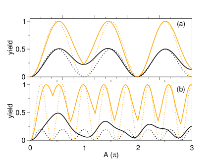
Figure 2: Maximum population transfer to the excited manifold at final time as a function of pulse area for a system with (a) $N_{i}=2$ and (b) $N_{i}=5$. In both cases $N_{f}=N_{i}$. Dotted lines represent results for degenerate structures while solid lines give results for structures with energy spacings $\Delta E=0.4\tau^{-1}$.

In Fig.2 we compare the results of the optimization with the yields obtained from the initial state $|i\rangle$ for degenerate structures $\Delta E=0$ and with constant energy spacing between adjacent levels $\Delta E=0.4\tau^{-1}$, for two different manifolds, $N_{c}=N_{i}=N_{f}=2$ and $N_{c}=N_{i}=N_{f}=5$. The optimal yields for degenerate structures follow the pattern of Rabi oscillations coinciding with the population transfer from the initial state, but with full population transfer at multiples of $\pi$ of the pulse area. For non-degenerate structures the minima of these oscillations does not drop to zero but increases with the number of levels, despite the $N^{-1}$ factor in Eq.(7).

It is interesting to analyze generic features of the optimized initial states. When the extended pulse area ${\cal A}_{e}=\sqrt{N_{i}N_{f}}{\cal A}$ is an odd multiple of $\pi$, the optimal initial states have a very clear structure: All their coefficients are equal. This result can be explained analytically for the degenerate structure, following exactly the same steps as in Eq.(1). We now define

$$|\Psi(t)\rangle=\bar{a}(t)\sum_{j}^{N_{p}}|g,1\rangle+\bar{b}(t)\sum_{k}^{N_{f}}|e,k\rangle+\bar{c}(t)\sum_{j}^{N_{u}}|g,j\rangle$$ (10)

where $\bar{a}(t)$ is the mean amplitude of all $N_{p}$ initially populated levels in the initial manifold, whereas $N_{u}=N_{i}-N_{p}$ is the set of unoccupied states. Together with the previously defined $|R\rangle$ and $|E\rangle$ collective states, the collective initial state

$$|I\rangle=\frac{1}{\sqrt{N_{p}}}\sum_{j}^{N_{p}}|g,j\rangle$$ (11)

forms a orthonormal set such that the Hamiltonian can be written as

$${\sf H}:=-\frac{1}{2}\sqrt{N_{f}}\Omega(t)\left(\sqrt{N_{p}}|I\rangle\langle E|+\sqrt{N_{u}}|E\rangle\langle R|+\mathrm{c.c.}\right)$$ (12)

with the same eigenvalues as before. Given the wave function $|\Psi(t)\rangle=A(t)|I\rangle+B(t)|E\rangle+C(t)|R\rangle$ with $A(t)=\sqrt{N_{p}}\,\bar{a}(t)$, the probability of reaching the excited manifold is

$$P_{E}(t)=\frac{N_{p}N_{i}}{N_{p}^{2}+N_{u}^{2}}\sin^{2}\left(\frac{1}{2}{\cal A}_{e}\right)$$ (13)

Whenever ${\cal A}_{e}(t)$ is an odd multiple of $\pi$, full population inversion can be achieved if all the sublevels of the initial manifold are equally populated and in phase. For different energy spacings other choices of phases and populations give better results, but the populations are always almost equal. On the other hand, it is simple to proof that when the initial probability amplitudes are all out of phase (such that $\sum_{j}^{N_{p}}a_{j}(0)=0$) then ${\cal F}$ is minimized and perfect transparency can be achieved, i.e. the population in the excited manifold is zero at all timesLIT . Similar results are obtained with nondegenerate structures although the transparency is no longer perfect. Since there are many more possible solutions that minimize the yield (exactly $N_{i}-1$ orthogonal eigenvectors for the degenerate structure) than those that maximize the yield (a single solution for the degenerate case) the set of eigenvalues fills from below and the subspace of population transfer is of very small dimension. From the point of view of quantum controllability, population transfer is a difficult problem. Nevertheless, other yields greather than zero can be achieved when $\Delta E\neq 0$.

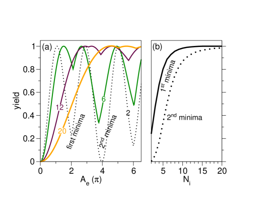
Figure 3: Maximum population transfer to the excited manifold at final time as a function of the extended pulse area for systems with different number of sublevels $N_{i}=N_{f}=N$ and fixed $\Delta E=0.4\tau^{-1}$. In (a) $N=2$ (dotted line), $N=5$ (green line), $N=20$ (orange line). In (b) we show how the first and second minima of the optimized yield increases with $N_{i}$. As shown in (a), the first minima for $N_{i}=20$ occurs practically at the first maxima for smaller $N_{i}$.

We now return to the original question: Do quantum structures help to control the dynamics? For population inversion between two manifolds, the problem is easily controllable by means of proper Rabi oscillations in the simplest case, with $N_{i}=N_{f}=1$. The existence of a substructure creates an effective detuning that reduces the oscillations. Therefore, the larger the energy spacing $\Delta E$ is, the smaller the back-effect of the unpopulated states and the more the system resembles a simple $2$-level system. However, by manipulating the state within the initial substructure one can regain full Rabi oscillations and reach a regime where the pulse area theorem is overcome with almost full controllability regardless of the pulse area for very large $N_{i}$. Fig.3(a) shows how the optimized yield with respect to changes in the initial state practically achieves full population inversion whenever $N_{c}=N_{i}$ is large. Fig.3(b) shows how the first (and second) minima of the optimal yield increase with $N_{i}$. Only in the degenerate case $N_{i}$ does not play any role and the dynamics is less controllable. Moreover, since the extended area increases with the number of sublevels, population inversion can be achieved with relatively weak pulsesfootnote2 . In the given example, with $N_{c}=N_{i}=N_{f}=20$, full inversion is obtained already with a pulse area of ${\cal A}\sim\pi/10$ (see Fig. 4). This is a consequence of parallel transfer.

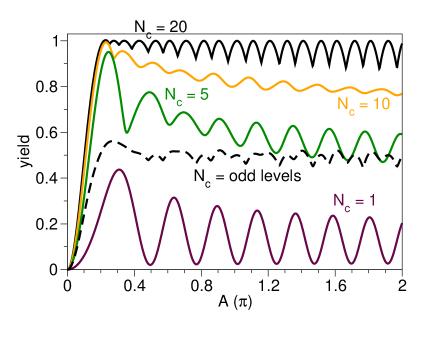
Figure 4: Maximum population transfer to the excited manifold at final time as a function of the pulse area for a system with $N_{i}=N_{f}=20$ sublevels with control on different subsets of the initial state, $N_{c}$.

On the other hand, one should remember that the ability to optimize the yield with increasing $N_{i}$ (for fixed $\Delta E$) is at the expense of a finer optimization of the initial state, where the optimal solution is typically a single one, while the “robust” subspace of near-zero eigenvalues occupies practically all the space of solutions. What happens when the dimensionality of the subspace that is controlled is smaller than the space that is initially accesible or, in other words, how are the solutions deteriorated when $N_{c}<N_{i}$? In Fig.4 we show the yield of population transfer as a function of the pulse area for different “control subspaces”. Now $N_{i}=20$ but the controller has only access to the first $N_{c}$ sublevels (or to the odd numbered sublevels, due to e.g. a unspecified selection rule or symmetry). The case $N_{c}=20$ gives maximum yield while $N_{c}=1$ implies no control over the initial state. The yields are deteriorated as the ability to control the system decreases and this effect cannot be overcome by increasing the pulse area. On the contrary, often best results are often obtained with ${\cal A}_{e}=\pi$. Moreover, adding external constraints, such as access to only odd number of levels, returns lower values of the yields.

In summary, we have shown that quantum substructures may hamper the success of population transfer in multi-level systems. By engineering the initial state one can avoid the detrimental effects and partially correct the Rabi oscillations of the yield forced by the pulse area theorem. This is not achieved by brute force (increasing the pulse areas) but by preparing quantum superposition states that cancel the detrimental Raman transitions and lead to parallel transfer. Full population blockade and in fact laser induced transparency can also be achieved in similar manners. The control over the dynamics increases with the ability to manipulate every sublevel of the quantum substructure and is substantially reduced when there is limited control over the sublevels.

References

- (1) S.A. Rice and M. Zhao, Optical Control of Molecular Dynamics (John Wiley & Sons, New York, 2000). M. Shapiro and P. Brumer, Quantum Control of Molecular Processes (Wiley-VCH, 2012). D. D’Alessandro, Introduction to Quantum Control and Dynamics (Chapman & Hall, 2007). C. Brif, R. Chakrabarti and H. Rabitz, Adv. Chem. Phys. Vol 148, 1 (2012).
- (2) G. M. Huang, T. J. Tarn, J. W. Clark, J. Math. Phys., 24 , 2608 (1983). V. Ramakrishna, M. V. Salapaka, M. Dahleh, H. Rabitz, A. Peirce, Phys. Rev. A, 51, 960 (1995). S. G. Schirmer, H. Fu and A. Solomon, Phys. Rev. A 63, 063410 (2001).
- (3) G. Turinici, H. Rabitz, Chem. Phys. 267, 1 (2001). G. Turinici, H. Rabitz, J. Phys. A, 2565 (2003).
- (4) J. S. Melinger, Suketu R. Gandhi, A. Hariharan, J. X. Tull, and W. S. Warren, Phys. Rev. Lett. 68, 2000 (1992). J. Cao, C. J. Bardeen, K. R. Wilson, Phys. Rev. Lett. 80, 1406 (1998). K. Bergmann, H. Theuer, B. W. Shore, Rev. Mod. Phys. 70, 1003 (1998). N. V. Vitanov, T. Halfmann, B. W. Shore, K. Bergmann, Annu. Rev. Phys. Chem. 52, 763 (2001). B. M. Garraway, K.-A. Suominen, Contemporary Physics 43, 97 (2002).
- (5) D. Townsend, B.J. Sussman, A. Stolow, J. Phys. Chem. A 115, 357, (2011).
- (6) B. W. Shore, Manipulating Quantum Structures Using Laser Pulses (Cambridge University Press 2011).
- (7) S. H. Autler and C. H. Townes, Phys. Rev. 100, 703 (1955).
- (8) B. Amstrup and N. E. Henriksen, J. Chem. Phys. 92, 8285 (1992). N. E. Henriksen, Adv. Chem. Phys. 91, 433 (1995). S. Meyer and V. Engel, J. Phys. Chem. A 101, 7749 (1997). N. Elghobashi and L. González, Phys. Chem. Chem. Phys. 6, 4071 (2004).
- (9) O.Kocharovskaya, Ya.I.Khanin, Sov. Phys. JETP 63, 945 (1986). K.J. Boller, A. Imamoglu, S. E. Harris, Phys. Rev. Lett. 66, 2593 (1991). Eberly, J. H., M. L. Pons, and H. R. Haq, Phys. Rev. Lett. 72, 56 (1994).
- (10) Obviously the minimization of the area of the pulse is at the expense of previous pulses that are needed to prepare the initial state.