Explicit inclusion of electronic correlation effects in molecular dynamics

Abstract

We design a quantum molecular dynamics method for strongly correlated electron metals. The strong electronic correlation effects are treated within a real-space version of the Gutzwiller variational approximation (GA), which is suitable for the inhomogeneity inherent in the process of quantum molecular dynamics (MD) simulation. We also propose an efficient algorithm based on the second-moment approximation to the electronic density of states for the search of the optimal variation parameters, from which the effective renormalized interatomic MD potentials are fully determined. By considering a minimal one-correlated-orbital Anderson many-particle model based on tight-binding hopping integrals, this fast GA-MD method is benchmarked with that using exact diagonalization to solve the GA variational parameters. In the infinite damping limit, the efficiency and accuracy are illustrated. This novel method will open up an unprecedented opportunity enabling large-scale quantum MD simulations of strongly correlated electronic materials.

I Introduction

Electronic correlation effects in materials such as transition metal oxides, give rise to emergent phenomena including Mott insulator, magnetism, heavy fermion, and unconventional superconductivity. These phenomena defy the description of the density functional theory (DFT) within local density approximation (LDA), which has been successful in describing electronic and structural properties of good metals and several semiconductors. Other discrepancies show up for materials like elemental actinide solids. For instance, the equilibrium volume of $\delta$-plutonium is experimentally 25% larger than the one given by the DFT-LDA approach, the greatest deviation known between experiment and theoretical value for this theory. The inadequacy of the DFT-LDA method for strongly correlated electron materials can be partly cured by including a direct treatment of quantum fluctuation effects by such quantum many-body approaches like the dynamical mean-field theory (DMFT). AGeorges96 ; GKotliar06 Together with its success in describing key physical observables in many strongly correlated electron materials, however, the LDA+DMFT is computationally expensive and in practice limited to solid state systems with high crystalline symmetry, making it time consuming to describe the structural relaxation problems. The combination of LDA with the Gutzwiller variational method Gutzwiller1963 ; Gutzwiller1965 has proved successful in providing an alternative but fast approach to the strongly correlated electron metals. Julien2006 When combined with the MD, the computational efficiency of the GA method makes it ideal for the studies of such problems as material structure stability in strongly correlated electron metals.

The strategy seems to be straightforward in principle. However, practical MD simulations for low symmetry structures (such as defects, surfaces, clusters, and liquids) containing thousands of atoms (and accompanying electrons) present challenges. On the one hand, for an explicit treatment of strong electronic correlation effects, the ab initio method requires a definition of local correlated orbitals. On the other hand, interatomic forces derived from the correlated wavefunctions need to be calculated rapidly and repeatedly during the time evolution of the MD trajectory. The aim of this work is to present a generic framework of the GA-MD method, together with a path forward for improving the computational speed of the GA optimization procedure. We propose the construction of such parameterizations as presented in the tight-binding electronic structure method, and the use of the semi-empirical second moment approximation of electronic density of states for the calculation of local kinetic energy. The latter will significantly speed up the minimization procedure in the Gutzwiller variational method for the electronic structure, opening up the possibility of MD simulations to strongly correlated electronic materials.

The outline of the paper is as follows. In Sec. II, we give a detailed description of the density matrix formulation of the Gutzwiller approximation. It has the advantage of being applicable to crystals, as well as topologically and/or chemically disordered systems. In Sec. III, we derive an approximate but analytical solution to the optimization equations in the GA, where a high quality fitted solution on the whole range of physical interest is provided, and propose the second moment approach to the electronic density of states for the calculation of kinetic energy parameters. In Sec. IV, this efficient GA-MD method is demonstrated in a minimal Anderson model for heavy fermion systems based on tight-binding hopping integrals. A concluding summary is given in Sec. V.

II Density matrix formulation of Gutzwiller method

II.1 Renormalization of hopping integrals

First, we review the Gutzwiller method briefly for which we closely follow Ref. Julien2006, but here we specifically include the topological disorder, i.e., during a typical MD process, no symmetry remains and all atoms are inequivalent. Among numerous theoretical approaches, the Gutzwiller method provides a transparent physical interpretation in terms of the atomic configurations of a given site. Originally, it was applied to the one-band Hubbard model Hamiltonian: Hubbard1963

$$H=H_{kin}+H_{int}\;,$$ (1)

with

$$H_{kin}=\sum_{i\neq j,\sigma}t_{ij}c_{i\sigma}^{\dagger}c_{j\sigma}\;,$$ (2)

and

$$H_{int}=U\sum_{i}n_{i\uparrow}n_{i\downarrow}\;.$$ (3)

The Hamiltonian contains a kinetic part $H_{kin}$ with a hopping integral $t_{ij}$ from site $j$ to $i$, and an interaction part with a local Coulomb repulsion $U$ for electrons on the same site. $c_{i\sigma}^{\dagger}$ ($c_{j\sigma}$) is the creation (annihilation) operator of an electron at site $i$ with up or down spin $\sigma$. $n_{i\sigma}=c_{i\sigma}^{\dagger}c_{i\sigma}$ measures the number (0 or 1) of electron at site $i$ with spin $\sigma$. The Hamiltonian, Eq. (1), contains the key ingredients for correlated up and down spin electrons on a lattice: the competition between delocalization of electrons by hopping and their localization by the interaction. It is one of the most widely used models to study the electronic correlations in solids.

In the absence of the interaction $U$, the ground state is characterized by the Slater determinant comprising the Hartree-like wave functions (HWF) of the uncorrelated electrons, $|\psi_{0}\rangle$. When $U$ is switched on, the weight of the doubly occupied sites will be reduced because of the cost of an additional energy $U$ per site. Accordingly, the trial Gutzwiller wave function (GWF) $|\psi_{G}\rangle$ is built from the HWF $|\psi_{0}\rangle$,

$$|\psi_{G}\rangle=g^{D}|\psi_{0}\rangle.$$ (4)

The role of $g^{D}$ is to reduce the weight of the configurations with doubly occupied sites, where $D=\sum_{i}n_{i\uparrow}n_{i\downarrow}$ measures the number of double occupations and $g\;(<1)$ is a variational parameter. This method corrects the mean field (Hartree) approach, for which up and down spin electrons are independent, and, overestimates configurations with doubly occupied sites. Using the Rayleigh-Ritz principle, this parameter is determined by minimization of the energy in the Gutzwiller state $|\psi_{G}\rangle$, giving an upper bound to the true unknown ground state energy of $H$. To enable a practical calculation, it is necessary to use the Gutzwiller approximation, which assumes that all configurations in the HWF have the same weight.

Nozieres Nozieres1986 proposed an alternative way which shows that the Gutzwiller approach is equivalent to the renormalization of the density matrix in the GWF. It can be formalized as

$$\rho_{G}=T^{\dagger}\rho_{0}T\;.$$ (5)

The density matrices $\rho_{G}=|\psi_{G}\rangle\langle\psi_{G}|$ and $\rho_{0}=|\psi_{0}\rangle\langle\psi_{0}|$ are projectors on the GWF and HWF, respectively. $T$ is an operator which is diagonal in the configuration basis; $T=\Pi_{i}T_{i}$ where $T_{i}$ is a diagonal operator acting on site $i$,

$$T_{i}|L_{i},L^{\prime}\rangle=\sqrt{\frac{p(L_{i})}{p_{0}(L_{i})}}|L_{i},L^{\prime}\rangle.$$ (6)

Here, $L_{i}$ is an atomic configuration of the site $i$, with probability $p(L_{i})$ in the GWF and $p_{0}(L_{i})$ in the HWF respectively, whereas $L^{\prime}$ is a configuration of the remaining sites of the lattice. Note that this prescription does not change the phase of the wave function as the eigenvalues of the operators $T_{i}$ are real. The correlations are local, and the configuration probabilities for different sites are independent.

The expectation value of the Hamiltonian is given by,

$$\langle H\rangle_{G}=\text{Tr}(\rho_{G}H)\;.$$ (7)

The mean value of the on-site operators is exactly calculated with the double occupancy probability, $d_{i}=\langle n_{i\uparrow}n_{i\downarrow}\rangle_{G}$. Therefore, $d_{i}$ is the new variational parameters replacing $g$. Using Eqs. (5)-(6), the two-site operator contribution of the kinetic energy can be written as,

$$\langle c_{i\sigma}^{\dagger}c_{j\sigma}\rangle_{G}=\text{Tr}(\rho_{G}c_{i\sigma}^{\dagger}c_{j\sigma})=\langle c_{i\sigma}^{\dagger}c_{j\sigma}\rangle_{0}\sum_{L_{-\rho}}\sqrt{\frac{p(L^{\prime}_{\sigma},L_{-\sigma})}{p_{0}(L^{\prime}_{\sigma})}}\sqrt{\frac{p(L_{\sigma},L_{-\sigma})}{p_{0}(L_{\sigma})}}\;,$$ (8)

where $L^{\prime}_{\sigma}$ and $L_{\sigma}$ are the only two configurations of spin $\sigma$ at sites $i$ and $j$ that give a non-zero matrix element for the operator in the brackets. The summation is performed over the configurations of opposite spin $L_{-\sigma}$. The probabilities $p_{0}$ in the HWF depend only on the number of electrons, whereas the $p$ in the GWF also depends on $d_{i}$.

After some elementary algebra, one can show that the Gutzwiller mean value can be factored into,

$$\langle c_{i\sigma}^{\dagger}c_{j\sigma}\rangle_{G}=\sqrt{q_{i\sigma}}\langle c_{i\sigma}^{\dagger}c_{j\sigma}\rangle_{0}\sqrt{q_{j\sigma}},$$ (9)

where these renormalization factors $q_{i\sigma}$ are local and can be expressed as

$$\sqrt{q_{i\sigma}}=\frac{\sqrt{1-n_{i\sigma}-n_{i-\sigma}+d_{i}}\sqrt{n_{i\sigma}-d_{i}}+\sqrt{d_{i}}\sqrt{n_{i-\sigma}-d_{i}}}{\sqrt{n_{i\sigma}(1-n_{i\sigma})}}\;.$$ (10)

In Eq. (9), $\langle c_{i\sigma}^{\dagger}c_{j\sigma}\rangle_{0}$ is shorthand for the expectation value of $c_{i\sigma}^{\dagger}c_{j\sigma}$ over the HWF $|\psi_{0}\rangle$, that is, $\langle\psi_{0}|c_{i\sigma}^{\dagger}c_{j\sigma}|\psi_{0}\rangle$, and similarly for the average over the Gutzwiller state $\Psi_{G}\rangle$. We have also used $n_{i\sigma}$ as shorthand for $\langle n_{i\sigma}\rangle$, that is, the average number of electrons on the considered “orbital-spin” in the HWF. In the simple case when the state is homogeneous and paramagnetic, all quantities becoming site- and spin-independent.

In Eq. (9), the term contributing to the kinetic energy, $\langle c_{i\sigma}^{\dagger}c_{j\sigma}\rangle_{0}$, is renormalized by a factor of $q$, which is less than one in the correlated state, and equal to one in the HWF. This factor can be interpreted as a direct measure of the correlation effect. Indeed Vollhardt Vollhardt1984 has shown that $1/q=m^{*}/m$ where $m^{*}$ is the effective mass and $m$ is the bare mass of the electron. Thus a $q$ close to $1$ corresponds to a weakly correlated electron system and a smaller $q$ value reflects enhancement of the correlation effect. Equation (7) leads to the variational energy per site, and for the homogeneous and paramagnetic state, is given by

$$E(d)=\langle H\rangle_{G}=2q\varepsilon^{0}_{kin}+Ud\;,$$ (11)

which can be minimized numerically with respect to the variational parameter $d$. In the above expression, the factor 2 accounts for the two-fold spin degeneracy and $\varepsilon^{0}_{kin}$ is the kinetic energy per site and per spin identical at all sites and spins for an homogeneous HWF,

$$\varepsilon^{0}_{kin}=\sum_{j}\langle c_{i\sigma}^{\dagger}c_{j\sigma}\rangle_{0}t_{ij}$$ (12)

In the case of half filling ($n=1/2$), minimization is analytical, and provides the optimal choice for double occupancy $d$

$$d=\frac{1}{4}\biggl{(}1-\frac{U}{16\varepsilon^{0}_{kin}}\biggr{)}\;,$$ (13)

and

$$q=1-\frac{U^{2}}{(16\varepsilon^{0}_{kin})^{2}}\;.$$ (14)

If the Coulomb repulsion $U$ exceeds a critical value $U_{c}=16\varepsilon^{0}_{kin}$, $q=0$, leading to an infinite quasiparticle mass with a Mott-Hubbard Metal-Insulator transition. This is also known as “the Brinkmann-Rice transition”, Brinkmann1970 as these authors first applied the Gutzwiller approximation to the Metal-Insulator transition.

Away from half-filling, one has to minimize the variational energy of Eq. (7) numerically. Moreover if the system is inhomogeneous, which is the case for a MD simulation, all quantities ($d_{i}$, $q_{i}$…) may vary locally from one site to the other. Consequently, the general variational energy, a function of double occupancy probabilities $d_{i}$ on all sites, is

$$E_{var}=\sum_{ij\sigma}\sqrt{q_{i\sigma}}t_{ij}\sqrt{q_{j\sigma}}\langle c_{i\sigma}^{\dagger}c_{j\sigma}\rangle_{0}+\sum_{i}U_{i}d_{i}$$ (15)

Minimization must then be performed numerically for each site, i.e., derivation with respect to $d_{i}$ , leading to the local equation:

$$\frac{\partial\sqrt{q_{i\sigma}}}{\partial d_{i}}=\frac{U_{i}}{4|e_{i\sigma}|}\;.$$ (16)

Here $e_{i\sigma}$ is the local partial “effective” kinetic energy, i.e., the contribution of orbital-spin “$i\sigma$” to kinetic energy, but calculated with an “effective” hopping, renormalized by $q$,

$$e_{i\sigma}=\sum_{j}\langle c_{i\sigma}^{\dagger}c_{j\sigma}\rangle_{0}t_{ij}\sqrt{q_{j\sigma}}$$ (17)

II.2 Inequivalent sites: renormalization of levels

When sites are inequivalent, or if orbitals belong to different symmetries as in a multiorbital basis, it is necessary to add to the Hamiltonian an on-site energy term

$$H_{on-site}=\sum_{i\sigma}\epsilon^{0}_{i\sigma}n_{i\sigma}$$ (18)

The Hubbard Hamiltonian is written as

$$H=\sum_{i\neq j,\sigma}t_{ij}c_{i\sigma}^{\dagger}c_{j\sigma}+\sum_{i\sigma}\epsilon^{0}_{i\sigma}n_{i\sigma}+U\sum_{i}n_{i\uparrow}n_{i\downarrow}$$ (19)

In this case, the starting HWF directly obtained from the non-interacting part of the Hamiltonian, is not automatically the optimal choice, i.e., having the lowest energy. For example, if we look for the ground state of Eq. (19) in the Hartree-Fock (HF) self-consistent field formalism, it is necessary to vary the orbital occupations. Practically, it can be achieved by replacing Eq. (19), by an effective Hamiltonian $H_{eff}$ of independent particles with renormalized on-site energies $\epsilon_{i\sigma}$:

$$H_{eff}=\sum_{i\neq j,\sigma}t_{ij}c_{i\sigma}^{\dagger}c_{j\sigma}+\sum_{i\sigma}\epsilon_{i\sigma}n_{i\sigma}+C\;.$$ (20)

The HWF we are looking for is an approximate ground state of the true many-body Hamiltonian (19) and is the exact ground state of effective Hamiltonian (20). The additive constant $C$ accounts for double counting energy reference, so that the ground state energies are the same for both Hamiltonians:

$$\langle H_{eff}\rangle=\langle H\rangle\;.$$ (21)

The optimal choice of parameters $\epsilon_{i\sigma}$ can be obtained by minimizing the ground state energy of $H_{eff}$ with respect to $\epsilon_{i\sigma}$ . With the help of Hellmann-Feyman theorem, one can obtain the derivative of the kinetic energy

$$\frac{\partial\langle H_{kin}\rangle}{\partial\epsilon_{i\sigma}}=-\sum_{j\neq i,\sigma}\epsilon_{j\sigma}\frac{\partial\langle n_{j\sigma}\rangle}{\partial\epsilon_{i\sigma}}\;.$$ (22)

On the other hand, differentiation of Eq. (21) in association with Eq. (22) and the mean field approximation $\langle n_{i\uparrow}n_{i\downarrow}\rangle\approx\langle n_{i\uparrow}\rangle\langle n_{i\downarrow}\rangle$ recovers the well-known formula for the on-site energies

$$\epsilon_{i\sigma}=\epsilon_{i\sigma}^{0}+U\langle n_{i-\sigma}\rangle\;,$$ (23)

where the constant $C$ is simply $-U\sum_{i}\langle n_{i\uparrow}\rangle\langle n_{i\downarrow}\rangle$.

In the Gutzwiller approach, the same argument about the variation of orbital occupation, i.e., flexibility on the HWF $|\psi_{0}\rangle$, is true. It is necessary to find a way to vary this Slater determinant, from which the GWF $|\Psi_{G}\rangle$ is generated, so that the Gutzwiller ground-state energy is a minimum. One needs to find an equivalent of Eq. (23) in the Gutzwiller context. The average value of Eq. (19) on a GWF is given by:

$$\langle\Psi_{G}|H|\Psi_{G}\rangle = \sum_{ij\sigma}t_{ij}\sqrt{q_{i\sigma}}\langle c_{i\sigma}^{\dagger}c_{j\sigma}\rangle_{0}\sqrt{q_{j\sigma}}+U\sum_{i}d_{i}$$ (24)

$$+\sum_{i\alpha\sigma}\epsilon^{0}_{i\sigma}\langle n_{i\sigma}\rangle_{0}\;.$$

Following the previous HWF self-consistent field approach, one can find an effective Hamiltonian $H_{eff}$ of independent particles having $|\psi_{0}\rangle$ as an exact ground state. This state $|\psi_{0}\rangle$ generates the GWF $|\Psi_{G}\rangle$ which is an approximate ground state of the true Hamiltonian Eq. (19). In analogy with Eq. (21),

$$\langle\psi_{0}|H_{eff}|\psi_{0}\rangle=\langle\Psi_{G}|H|\Psi_{G}\rangle\;,$$ (25)

leads to the expression:

$$H_{eff}=\sum_{i\neq j,\sigma}\tilde{t}_{ij}c_{i\sigma}^{\dagger}c_{j\sigma}+\sum_{i\sigma}\epsilon_{i\sigma}n_{i\sigma}+C^{\prime}\;,$$ (26)

with effective but fixed renormalized hopping integrals $\tilde{t}_{ij}=\sqrt{q_{i\sigma}}t_{ij}\sqrt{q_{j\sigma}}$ and effective on-site energies $\epsilon_{i\sigma}$, still to be determined. The Hellmann-Feynman theorem applied to $H_{eff}$ provides again an expression similar to Eq. (22), but with effective hopping integrals. Taking into account the dependence of the ${q_{i\sigma}}$’s through ${n_{i\sigma}}$ (Eq. (10)) and differentiating Eqs. (24) and (25) with respect to the parameters $\epsilon_{i\sigma}$, one obtains the equivalent expression to Eq. (23) in the Gutzwiller context:

$$\epsilon_{i\sigma}=\epsilon^{0}_{i\sigma}+2e_{i\sigma}\frac{\partial\ln(\sqrt{q_{i\sigma}})}{\partial n_{i\sigma}}\;.$$ (27)

Here $e_{i\sigma}$ is the partial kinetic energy of orbital-spin $i\sigma$

$$e_{i\sigma}=\sum_{j\sigma}\tilde{t}_{ij}\langle c_{i\sigma}^{\dagger}c_{j\sigma}\rangle_{0}=\int_{-\infty}^{\rm E_{F}}E\tilde{N}_{i\sigma}(E)dE-\epsilon_{i\sigma}\langle n_{i\sigma}\rangle_{0}\;,$$ (28)

with $\tilde{N}_{i\sigma}$ the $i\sigma$-projected density of states (DOS) for a system described $H_{eff}$. Equation (25) leads to

$$C^{\prime}=U\sum_{i}d_{i}-\sum_{i\sigma}2e_{i\sigma}\frac{\partial\ln(\sqrt{q_{i\sigma}})}{\partial n_{i\sigma}}\langle n_{i\sigma}\rangle\;.$$ (29)

Except for a few very special conditions in one-band Hubbard model, the renormalization of correlated-orbital levels is not only important in the optimization of the total energy but also in giving a correct description of single-particle quasiparticle properties. JXZhu2012 To solve the full problem of finding an approximate ground state to Eq. (19), one is faced with a self-consistency loop: First get the occupations $\langle n_{i\sigma}\rangle_{0}$ from a HWF, and a set of ‘bare’ $\epsilon^{0}_{i\sigma}$ levels; then obtain a set of configuration parameters, the probabilities of double occupation, $d_{i}$ by minimizing Eq. (24) with respect to these probabilities, followed by the on-site level renormalization according to Eq. (27). The loop repeated until a convergence is achieved.

III Approximated solutions of minimization equations

Due to the complicated expression of Eq. (10), it is non-trivial to solve Eq. (16). Graphically, the solution corresponds to the intersection of the function $\frac{\partial\sqrt{q_{i\sigma}}}{\partial d_{i}}$ with a horizontal line $U/4|e_{i\sigma}|$ (see Fig. 1).

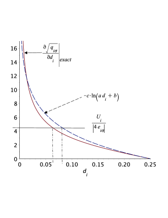
Figure 1: (Color online) The exact (full line) and approximate (dashed line) $\partial\sqrt{q_{i\sigma}}/\partial d_{i}$ as a function of $d_{i}$.

This situation may seem insurmountable for application of the Gutzwiller method to MD, as analytical expressions are necessary to be able to derive forces. Fortunately, the function $\frac{\partial\sqrt{q_{i\sigma}}}{\partial d_{i}}$ can be fitted with reasonable accuracy (see Fig. 1) by a logarithm function, giving an analytical approximate solution $d_{i}$ of Eq. (16). This choice was suggested by the shape of the true derivative of $\sqrt{q_{i\sigma}}$ , keeping in mind the following physical constraints: The uncorrelated case ($U=0$) has to give the solution $d_{i}=n_{i\sigma}^{2}$, for a given occupancy $n_{i\sigma}$, and the probability of double occupancy $d_{i}$ is restricted in the range $\text{max}(0,2n_{i\sigma}-1)<d_{i}<n_{i\sigma}$ (otherwise there would be negative arguments in the square root of $q$), providing a rescaling of the logarithm argument. Finally, we adapt the coefficient in front of the logarithm, in such a way that the fitted function has the same slope as the true one in the uncorrelated limit $n_{i\sigma}^{2}$. The final result reads:

$$\frac{\partial\sqrt{q_{i\sigma}}}{\partial d_{i}}\simeq-c\ln(ad_{i}+b)$$ (30)

The physical constraints above fix uniquely all three coefficients

$$a = \frac{1}{n_{i\sigma}^{2}-\text{max}(0,2n_{i\sigma}-1)}\;,$$ (31)

$$b = -a\;\text{max}(0,2n_{i\sigma}-1)\;,$$ (32)

$$c = \frac{n_{i\sigma}^{2}-\text{max}(0,2n_{i\sigma}-1)}{4n_{i\sigma}^{3}(1-n_{i\sigma})^{3}}\;.$$ (33)

The approximate value of double occupancy, the solution of minimization equation, within this approximation, is $d_{i}=(n_{i\sigma}^{2}-d_{m})\exp(-U_{i}/|4e_{i\sigma}|)-d_{m}$, where $d_{m}=\text{max}(0,2n-1)$. The small remaining difference between this approximate and the true value can be corrected by a second order expansion around the approximate value $d_{i}$ leading to an accurate analytical expression

$$d_{i}^{2nd}=d_{i}-\frac{f^{\prime}+\sqrt{f^{\prime 2}-2f^{\prime\prime}[f+c\ln(ad_{i}+b)]}}{f^{\prime\prime}}\;.$$ (34)

Here $f$, $f^{\prime}$, and $f^{\prime\prime}$ stand for the true $\frac{\partial\sqrt{q_{i\sigma}}}{\partial d_{i}}$, and its first and second order derivatives, respectively, calculated at the approximated value $d_{i}$.

The relative error on this second order corrected value with respect to the exact solution is less than 1% over the whole range of values. This second order corrected local double occupancy is the one now used in the calculation of renormalization factor $\sqrt{q_{i\sigma}}$, Eq. (10). To check the validity of this approximation for the derivative, we also plot in Fig. 1 the comparison between true and approximate $\sqrt{q_{i\sigma}}$. Again we see the good accuracy, the small discrepancy being in the range of very small double occupancy, i.e., corresponding to high value of Coulomb repulsion $U$, which are far from the values for realistic materials.

The other input for Eq. (28) necessary to perform tractable MD simulations is the partial energy. A common approximation is the well-known approach of second moments JFriedel:1964 with the assumption of a rectangular electronic density of states of bandwidth $W_{i\sigma}$ and height $1/W_{i\sigma}$ for each spin. The resulting second moment of the rectangular band is $\mu_{2,i}=W^{2}_{i\sigma}/12$. For a given MD snapshot, the second moment for a given atomic site “$i$” can be constructed as a sum over atoms “$j$” neighboring “$i$” as $\mu_{2,i}=\sum_{j}t_{ij}^{2}$ (see Appendix for more details). Using the simple tight-binding theory, WAHarrison:1980 the hopping integrals $t_{ij}$ scale as a power law of the interatomic distance $r_{ij}=|\mathbf{r}_{i}-\mathbf{r}_{j}|$. With the number of electrons on each atom (assuming charge neutrality for all sites), the partial kinetic energy needed as input in Eq. (28) and is given by $e_{i\sigma}=W_{i\sigma}n_{i\sigma}(n_{i\sigma}-1)/2$, similar to the result by Ackland. Ackland2003 To compute $\mu_{2}$ and to account for the effect of Coulomb correlations, we use the hopping integrals, renormalized by $q$-factors, $\sqrt{q_{i}}t_{ij}\sqrt{q_{j}}$, rather than the bare ones, $t_{ij}$: After minimization in the Gutzwiller method, the true interacting Hamiltonian $H$, is replaced by an effective Hamiltonian of non-interacting quasiparticles, with renormalized hopping integrals (and potentially renormalized on-sites too, but it is useless in our case, as we assumed charge neutrality, so there are no average charge transfer between sites). To conclude, we see that inclusion of electronic correlations in MD simulations within the Gutzwiller method, just requires one more intermediate step, compared to usual one, for having the renormalization factors that reduce a bit the hopping integrals. Once they have been computed for a set of actual positions of atoms, the rest of the process is similar to the usual way developed in other semi-empirical approaches. MFinnis:1984 ; MSDaw:1983

IV Model and results

IV.1 Model

To illustrate the possibility of the method, we consider a minimal two-orbital model that mimics, e.g., heavy fermions or actinides systems, with one non-correlated band, called for convenience “d”, whereas the other, called “f”, bears a strong local Coulomb repulsion $U$. For simplicity, each of these two orbitals has a spin-$\frac{1}{2}$ degree of freedom per site. This model is described by the following Hamiltonian (close in spirit to the Anderson lattice model) with the usual notation:

$$H = \sum_{i,j,\sigma}t_{i\textit{d},j\textit{d}}c_{i\textit{d}\sigma}^{\dagger}c_{j\textit{d}\sigma}+t_{i\textit{d},j\textit{f}}c_{i\textit{d}\sigma}^{\dagger}c_{j\textit{f}\sigma}+t_{i\textit{f},j\textit{d}}c_{i\textit{f}\sigma}^{\dagger}c_{j\textit{d}\sigma}$$ (35)

$$+\sum_{i\sigma}(\epsilon^{0}_{i\textit{d}\sigma}n^{\textit{d}}_{i\sigma}+\epsilon^{0}_{i\textit{f}\sigma}n^{\textit{f}}_{i\sigma})$$

$$+\sum_{i}U_{i}n^{\textit{f}}_{i\uparrow}n^{\textit{f}}_{i\downarrow}\;.$$

Here the $d$-orbitals are coupled among themselves and with $f$-orbitals, whereas the $f$-orbitals are only coupled to their neighboring $d$-orbitals. The power laws WAHarrison:1984 in distance from atom located at position $r_{i}$ to atom at $r_{j}$ for hopping integrals are -5 and -6 for dd-coupling and df-coupling, respectively:

$$t_{i\textit{d},j\textit{d}}=\frac{t_{dd,0}}{|r_{i}-r_{j}|^{5}}\;,$$ (36)

and

$$t_{i\textit{d},j\textit{f}}=\frac{t_{df,0}}{|r_{i}-r_{j}|^{6}}\;,$$ (37)

where $t_{dd,0}$ and $t_{df,0}$ are constants. After a Gutzwiller mean-field treatment of Hamiltonian Eq. (35), we obtain

$$H_{eff} = \sum_{i,j,\sigma}t_{i\textit{d},j\textit{d}}c_{i\textit{d}\sigma}^{\dagger}c_{j\textit{d}\sigma}+\sum_{i,j,\sigma}[t_{i\textit{d},j\textit{f}}\sqrt{q_{j}}c_{i\textit{d}\sigma}^{\dagger}c_{j\textit{f}\sigma}+\text{H.c.}]$$ (38)

$$+\sum_{i\sigma}(\epsilon^{0}_{i\textit{d}\sigma}n^{\textit{d}}_{i\sigma}+\epsilon_{i\textit{f}\sigma}n^{\textit{f}}_{i\sigma})+\sum_{i}U_{i}d_{i}+C^{\prime}\;,$$

whose parameters are obtained from the minimization procedure analogous to deriving Eq. (26) from Eq. (25), for a given set of atomic positions. When the converged Gutzwiller ground state has been obtained we calculate the forces on each atom. These attractive forces have a quantum origin, due to the hybridization through hopping integrals. To mimic the short range repulsion that accounts for the Pauli principle when atoms get too close, we add a phenomenological repulsive potential

$$E_{\text{rep}}=\frac{1}{2}\sum_{ij}\frac{\Lambda_{0}}{|\mathbf{r}_{i}-\mathbf{r}_{j}|^{12}}$$ (39)

with $\Lambda_{0}$ a constant.

IV.2 Calculation of forces

For a given set of atomic positions, the overall total energy of the system is the sum of the electronic approximate Gutzwiller ground state energy $E_{G}$ plus the short range repulsion potential,

$$E_{tot}=E_{G}+E_{\text{rep}}\;.$$ (40)

The $x$- component of the force acting on atom $i$, $F_{x,i}$ is the derivative of $E_{tot}$ with respect to position component $x_{i}$ of this atom (same relations hold for $y$- and $z$-components):

$$F_{x,i}=-\frac{\partial E_{tot}}{\partial x_{i}}=-\frac{\partial E_{G}}{\partial x_{i}}-\frac{\partial E_{\text{rep}}}{\partial x_{i}}\;.$$ (41)

From the Hellmann-Feynman theorem, the first term, due to hybridization, can be split into elementary contributions:

$$-\frac{\partial E_{G}}{\partial x_{i}}=\sum_{j\neq i}\sum_{\alpha\beta}f^{(x)}_{i\alpha j\beta}$$ (42)

where the contribution of orbitals $\alpha$ of site $i$ and $\beta$ of site $j$ ($\alpha$ or $\beta$ are either $d$- or $f$-orbitals) is related to the derivative of the hopping integral $t_{i\alpha j\beta}$,

$$f^{(x)}_{i\alpha j\beta}=-\frac{\partial t_{i\alpha j\beta}}{\partial x_{i}}4\sqrt{q_{i}}\langle c_{i\alpha\sigma}^{\dagger}c_{j\beta\sigma}\rangle\sqrt{q_{j}}\;.$$ (43)

The factor 4 arises from the two-fold spin degeneracy and the Hermiticity. For the interacting case ($U\neq 0$), $\sqrt{q_{i}}$ or $\sqrt{q_{j}}$ are less than one for $f$-orbitals but equal to one for $d$-orbitals. For the non-interacting case ($U=0$), the above formula is obtained by setting all $q=1$. It can be shown that forces from the hybridization origin are always attractive.

The computed forces Eq. (41) are then inserted into New’s equation of motion (EOM) for each atom. The positions are advanced in time by a time step $\delta t$ by numerically integrating the EOMs with the Verlet algorithm. The resulting new atomic positions are then taken as input into Eq. (38), and new atomic forces Eq. (41) are computed. The MD trajectory consists of the string of many time steps iterating back and forth through this two-step process.

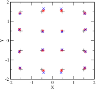
Figure 2: (Color online) Comparison of atomic positions for the second moment method (red ‘$\ast$’) and exact diagonalization (blue ‘$\times$’) for the non-interacting case. Initial positions (black ‘$+$’) are also plot.

IV.3 Results

As a demonstration, consider a two-dimensional system that contains 16 atoms. In the calculation, we take $t_{dd,0}=-1t$, $t_{df,0}=0.5t$, and $\Lambda_{0}=0.4t$. Hereafter all energies are measured in units of $t$. The bare $f$ level is chosen to be $\epsilon_{if\sigma}^{0}=-U/2$. The initial condition is 16 atoms forming a regularly spaced 4 x 4 array with a unit nearest-neighbor distance. To benchmark our method and see the efficiency of second moment plus accurate approximate solution for double occupancy, we also performed the calculation based on exact diagonalization. Since we are interested in finding only the equilibrium structure of the system, the velocity on each atom is set to zero before advancing by $\Delta t$ the numerical solution of the EOM. The resulting MD “trajectory” eventually finds a local minimum on the energy landscape as the atomic positions are converged and the residual forces are driven to the noise limit. We started with the non-interacting case ($U=0$). Figure 2 shows initial and final positions of of atoms after 5 millions of MD time steps i.e., sufficient to converge and where residual forces can be considered as noise. The equilibrium structures obtained from the second moment and the exact diagonalization methods are quite similar with the root mean square deviation $\Delta r_{\text{RMS}}=\sqrt{\sum_{i=1}^{N}(\mathbf{r}^{\text{sm}}_{i}-\mathbf{r}^{\text{ED}}_{i})^{2}/N}$ of only about 0.058 unit distance. The CPU time in the case of second moment method is a factor of 20 times faster than the exact diagonalization. The second moment approach scales linearly with the number of atoms $N$ whereas ED scales as $N^{3}$. Therefore, if we had studied 10 times more particles, i.e., 160, the increase speed factor would have been around 2000. The combination of second moment for approximate electronic structure quantities and a fast Gutzwiller solver really opens the realm of possibilities for the simulations of large systems, where electronic correlations play an important role.

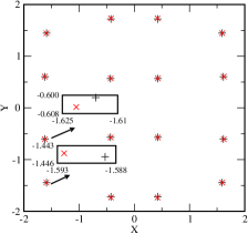
Figure 3: (Color online) Comparison of atomic positions after MD process for second moment method for $U=0$ non-interacting case (black ‘$+$’) and for $U=4t$ Gutzwiller interacting case (red ‘$\times$’). The expansion is small but can be seen in the zoom-in insets.

We then started from the converged atomic positions as shown in Fig. 2 and repeated the simulation with a local Coulomb repulsion $U=4t$. The comparison between $U=0$ and $U=4t$ for the second moment approach is displayed in Fig. 3. As expected and in accordance to our previous experience with Pu-$\delta$, Julien2006 we see that the Gutzwiller $q$-factors have the effect of reducing the hybridization and the resultant attractive forces, which leads to a slightly more expanded equilibrium structure as shown in the zoom-insets of Fig. 3. The same trend was also observed in the results (not shown here) obtained by exact diagonalization with $U=0$ versus $U=4t$. We note that the structure expansion is quite small. The reason lies in the fact that in the Anderson-like model, the attractive force is contributed not only from the $d$-$f$ hybridization hopping but also significantly from the direct $d$-$d$ hopping. In addition, the efficiency of the hybridization reduction in the present model is proportional to $\sqrt{q_{i}}$. It is in contrast to the one-orbital Hubbard model, where the effective hopping integrals are proportional to $\sqrt{q_{i}}\sqrt{q}_{j}$.

V Summary and conclusion

We have derived for the first time a real-space version of the Gutzwiller method embedded into the MD simulations for strongly correlated electron systems. From the positions of a configuration of atoms, a Hamiltonian can be constructed in terms of hopping integrals, on-site energies and Coulomb repulsion terms. It is precisely these interaction terms that require treatment beyond mean-field HF theories, which allows for Gutzwiller method. This method is a variational method in the Rayleigh-Ritz sense, for which one minimizes the energy of the system via a set of local Gutzwiller variational parameter dependent on each site, thereby providing an approximate ground state energy for the system. This minimization can be computationally demanding, especially when all the sites are inequivalent. This has motivated the development of an accurate analytical solution for finding the optimized double occupancy on each site.

MD simulation is a repeated two step process. First, employing a Hellmann-Feynman theorem within the Gutzwiller ground state, we can calculate the quantum origin of the forces acting on the atoms. This ground state energy defines an interatomic potential, which explicitly accounts for correlation effects. Second, the atomic forces derived from this interatomic potential are input into the classical equations of motion and the atomic positions are evolving forward in time for one time step using a numerical integrator (e.g., the Verlet algorithm). The step one is then repeated, where the new atomic positions define a new Hamiltonian whose new ground state can be found by the Gutzwiller method and so on.

A further approximation consists of avoiding exact diagonalization of the Hamiltonian from which, in principle, we can calculate the local densities of states (DOS) to obtain all necessary integrated quantities. Instead, we have proposed to use the second moment approximation, in which the true DOS is replaced by a rectangular approximation having the same second moment. Because the needed quantities to construct the variational ground state energy are basically integrated from DOS, they are less sensitive to the detailed structure of the DOS, thus validating the second moment approximation. The second moment of the energy is easily computed from a few Hamiltonian matrix elements, where we can set up the MD process without invoking exact diagonalization to solve iteratively the Gutzwiller minimization. Therefore, a very accurate approximate, but analytical solution, is available, making this process feasible. We concluded this first study with an application to a realistic case to show the potential of this approach, which to our knowledge, has never been developed and will open up new possibilities for simulations of correlated electron materials with molecular dynamics. We have applied the Gutzwiller Molecular Dynamics method to the one correlated orbital per site case as exemplified in the lattice Anderson model. The generalization of these ideas to multiple correlated orbitals case is not made directly because of higher degeneracy. That is, the number of variational parameters increases as the number of atomic configurations (namely as $2^{G}$, with $G$ the degeneracy of the level) and therefore the number of local equations to be solved increases accordingly. We defer to future work on how to reduce the number of variational parameters, and as in the one correlated orbital per site model, to find an analytical approach to the problem.

*

Appendix A Second moment approximation for bond quantities

We follow closely the derivation by Pettifor and co-workers APSutton:1988 ; DGPettifor:1989 for the bond order in a tight-binding model. To compute forces from the derivation of Hamiltonian, one needs average values like $\langle c^{{\dagger}}_{i}c_{j}\rangle$, with $i$ and $j$ being a short hand for site and spin-orbital states. Within these notations, and for the purpose of demonstration, we write the Hamiltonian $H$ in simple tight-binding form:

$$H=\sum_{i\neq j}t_{ij}c_{i}^{\dagger}c_{j}+\sum_{i}\epsilon_{i}n_{i\sigma}\;,$$ (44)

where on-site energies $\epsilon_{i}=\langle i|H|i\rangle$ can be identified as average value of the Hamiltonian on local state labelled by $i$ whereas hopping integrals $t_{ij}=\langle i|H|j\rangle$ couple states $i$ to $j$. The bracket is the thermal average obtained for a general operator $O$ by

$$\langle O\rangle=Tr\frac{e^{-\beta(H-\mu N)}O}{Z}\;,$$ (45)

where $H$, $\mu$, $N$ and $Z$ are respectively the Hamiltonian, the chemical potential, the operator number of particles and the grand partition function. This average reduces to the ground state mean value at zero temperature. From exact diagonalization (as we do for the cluster example developed here), these quantities can easily be calculated from the weights $w(j,n)$ of state $j$ (and similarly $i$) on eigenstate labelled by $n$ and of energy $\epsilon_{n}$:

$$\langle c^{{\dagger}}_{i}c_{j}\rangle=\sum_{n}f(\epsilon_{n})w^{*}(i,n)w(j,n)\;,$$ (46)

where $f(\epsilon_{n})$ is the Fermi distribution.

For large systems, where the speed of calculation is a limiting factor, it might be desirable however to avoid this diagonalization, and to find an approximate but cheap way to get them. In a alternative route, they are obtained from the retarded Green function (with Zubarev notation Zubarev60 ) $\mathcal{G}_{i,j}(\omega)\equiv\langle\langle c_{j};c^{{\dagger}}_{i}\rangle\rangle_{\omega}$, which is the Fourier transform of $\mathcal{G}_{i,j}(t)=-i\theta(t)\langle\{c_{j}(t),c^{{\dagger}}_{i}(0)\}\rangle$ for the operators $c_{j}$ and $c^{{\dagger}}_{i}$. $\mathcal{G}_{i,j}(\omega)$ can be considered as an off-diagonal element of the Green function, and in the case of effective independent electrons (with only 1-body operators, as it is the case for effective Hamiltonians) it reduces to the usual resolvent:

$$(\omega-H)\mathcal{G}=I\;,$$ (47)

The diagonal element (i.e. same states $i$ and $j$) relates to the $i$-projected density of states $N_{i}(\omega)$ via:

$$N_{i}(\omega)=-\frac{1}{\pi}\text{Im}\mathcal{G}_{i,i}(\omega)\;.$$ (48)

There are several useful relations and sum rules that fulfills the Green function (see Ref. Zubarev60, for demonstration):

$$-\frac{1}{\pi}\int\text{Im}\langle\langle c_{j};c^{{\dagger}}_{i}\rangle\rangle_{\omega}d\omega = \langle\{c_{j},c^{{\dagger}}_{i}\}\rangle$$ (49)

$$= \delta_{i,j}\;,$$

and the so-called spectral theorem provides a direct way to compute the average values we are looking for:

$$-\frac{1}{\pi}\int f(\omega)\text{Im}\langle\langle c_{j};c^{{\dagger}}_{i}\rangle\rangle_{\omega}d\omega = \langle c^{{\dagger}}_{i}c_{j}\rangle\;.$$ (50)

When there is no magnetic field, the following relation holds:

$$\langle\langle c_{i};c_{j}^{{\dagger}}\rangle\rangle=\langle\langle c_{j};c^{{\dagger}}_{i}\rangle\rangle\;.$$ (51)

The main idea in the present approximate calculation is the following: we express exactly the off-diagonal element of Green function as a linear combination of diagonal elements of Green functions of bonding and anti-bonding states,created by $c^{{\dagger}}_{B\,or\,A}=\frac{c^{{\dagger}}_{i}\pm c^{{\dagger}}_{j}}{\sqrt{2}}$. Indeed, one can easily show

$$\mathcal{G}_{i,j}=\frac{1}{2}(\mathcal{G}_{B,B}-\mathcal{G}_{A,A})\;,$$ (52)

from which the desired quantity is obtained thanks to relations (50), (48) and (51):

$$\langle c^{{\dagger}}_{i}c_{j}\rangle=-\frac{1}{2\pi}\int f(\omega)(N_{B}(\omega)-N_{A}(\omega))d\omega\;.$$ (53)

Then the second moment approximation is applied to the DOS –the imaginary part of Green function– calculated for bonding and anti-bonding states, respectively. The second moment approximation is based on the constraints that all necessary quantities are integrated quantities. Consequently, they are not sensitive to the fine details of the DOS, which will be replaced by rectangular DOS having the same second moment that the true ones. The rectangular $i$-projected (centered on site energy $\varepsilon_{i}$ with width $W_{i}$ and height $1/W_{i}$) DOS has its second moment given by: $\varepsilon^{2}_{i}+W^{2}_{i}/12$ whereas a direct path-counting (see Ref. Cyrot-Lackmann73, ) gives $\varepsilon^{2}_{i}+\sum_{j\neq i}t^{2}_{ij}$. Identification between those two relations fixes uniquely the bandwidth $W_{i}$, from which the approximated $i$-projected DOS can be computed. This procedure has been widely used in semi-empirical molecular dynamics as in Ref. Ackland2003, , for approximate local DOS. The extension we suggest here is to used it also for the bonding and anti-bonding DOS, $N_{B}(\omega)$ and $N_{A}(\omega)$, to obtain the bond quantities.

It should be noted that in the particular case of the second moment of the projected density of states on A (or B), the second moment defined by the mean value $\langle A|H^{2}|A\rangle$ provides unusual terms as follows:

$$\mu_{2,ij}=\langle i|H^{2}|j\rangle=\sum_{k}\langle i|H|k\rangle\langle k|H|j\rangle\;.$$ (54)

Such terms do not appear in the traditional way of calculating the moments starting from a given orbital at a specific site $i$, where the second moment is simply given by the number of paths starting from $i$, returning after two jumps back to the same site: this later simpler case is obtained by setting $i=j$ in the last equation. Finally, we get the second moment on either $\mu_{2,AA}$ or $\mu_{2,BB}$ combination:

$$\mu_{2,AA}=\langle A|H^{2}|A\rangle=\frac{1}{2}(\mu_{2,ii}+\mu_{2,jj}-2\Re\mu_{2,ij})\;,$$ (55a)

$$\mu_{2,BB}=\langle B|H^{2}|B\rangle=\frac{1}{2}(\mu_{2,ii}+\mu_{2,jj}+2\Re\mu_{2,ij})\;,$$ (55b)

together with the center of band $\epsilon_{A}$ (resp. $\epsilon_{B}$ ):

$$\epsilon_{A} = \langle A|H|A\rangle=\epsilon_{i}+\epsilon_{j}-2\Re t_{ij}\;,$$ (56a)

$$\epsilon_{B} = \langle B|H|B\rangle=\epsilon_{i}+\epsilon_{j}+2\Re t_{ij}\;,$$ (56b)

from which we can obtain the related bandwidth $W_{A}=\sqrt{12(\mu_{2,AA}-\epsilon^{2}_{A})}$ (similar expression holds for $W_{B}$). Finally using expression (53) for rectangular DOS $N_{A}$ and $N_{B}$, we have the desired quantity:

$$\langle c^{{\dagger}}_{i}c_{j}\rangle=\frac{E_{F}-\epsilon_{B}}{2W_{B}}-\frac{E_{F}-\epsilon_{A}}{2W_{A}}\;,$$ (57)

where $E_{F}$ is the chemical potential at zero temperature. All this demonstration can be straightforwardly be extended to multiband case adding orbital index and spin to labels $i$ and $j$. This procedure presents the great advantage of being very rapid compared to exact diagonalization and one can check that the Green function related to approximate DOS also fulfills sum rule as given in Eq. (49).

References

- (1) A. Georges, G. Kotliar, W. Krauth, and M. J. Rozenberg, Rev. Mod. Phys. 68, 13 (1996).
- (2) For a review, see G. Kotliar, S. Y. Savrasov, K. Haule, V. S. Oudovenko, O. Parcollet, C. A. Marianetti, Rev. Mod. Phys. 78, 865 (2006).
- (3) M.C. Gutzwiller, Phys. Rev. Lett. 10, 159 (1963).
- (4) M.C. Gutzwiller, Phys. Rev. 137, A1726 (1965).
- (5) J.-P. Julien and J. Bouchet, Prog. Theor. Chem. Phys., B 15 , 509-534 (2006)
- (6) J. Hubbard, Proc. Roy. Soc. London, A 276, 238 (1963).
- (7) P. Nozières, Magnétisme et localisation dans les liquides de Fermi, Cours du Collège de France, Paris (1986).
- (8) D. Vollhardt, Rev. Mod. Phys., 56, 99 (1984).
- (9) W.F. Brinkmann and T.M. Rice, Phys. Rev. B, 2, 1324 (1970).
- (10) J.-X. Zhu, J.-P. Julien, Y. Dubi, and A. V. Balatsky, Phys. Rev. Lett. 108, 186401 (2012).
- (11) J. Friedel, Trans. Metall. Soc. AIME 230, 616 (1964).
- (12) W. A. Harrison, Electronic Structure and the Properties of Solids (W. H. Freeman and Co., San Francisco, 1980).
- (13) G. J. Ackland and S. K. Reed, Phys. Rev. B 67, 174108 (2003).
- (14) M. Finnis and J. F. Sinclair, Phil. Mag. A 50, 45 (1984).
- (15) M. S. Daw and M. I. Baskes, Phys. Rev. Lett. 50, 1285 (1983).
- (16) J. Bünemann, W. Weber and F. Gebhard, Phys. Rev. B 57, 6896 (1998).
- (17) J. Bünemann, F. Gebhard, and W. Weber, J. Phys.: Condens. Matter, 9, 7343 (1997).
- (18) J. Bünemann, and W. Weber, Phys. Rev. B 55, 4011 (1997).
- (19) T. Okabe, J. Phys. Soc. Jpn. 66, 2129 (1997).
- (20) H. Hasegawa, J. Phys. Soc. Jpn. 66, 1391 (1997).
- (21) J.P. Lu, Inter. J. Mod. Phys. B10, 3717 (1996).
- (22) S.Y. Savrasov and G. Kotliar, Phys. Rev. Lett. 84, 3670 (2000).
- (23) F. Gebhard, Phys. Rev. B 44, 992 (1991).
- (24) D.N. Zubarev, Soviet Phys. Uspeskhi 3, 320(1960).
- (25) J.P. Gaspard and F. Cyrot-Lackmann, J. Phys. C: Solid State Phys. 6, 3077 (1973).
- (26) A. P. Sutton, M. W. Finnis, D. G. Pettifor, and Y. Ohta, J. Phys. C: Solid State Phys. 21, 35 (1988).
- (27) D. G. Pettifor, Phys. Rev. Lett. 63, 2480 (1989).