Evolutionary outcomes for pairs of planets undergoing orbital migration and circularization: second order resonances and observed period ratios in Kepler’s planetary systems

Abstract

In order to study the origin of the architectures of low mass planetary systems, we perform numerical surveys of the evolution of pairs of coplanar planets in the mass range $(1-4)\ \mathrm{M}_{\oplus}.$ These evolve for up to $2\times 10^{7}\mathrm{yr}$ under a range of orbital migration torques and circularization rates assumed to arise through interaction with a protoplanetary disc.

Near the inner disc boundary, significant variations of viscosity, interaction with density waves or with the stellar magnetic field could occur and halt migration, but allow circularization to continue. This was modelled by modifying the migration and circularization rates.

Runs terminated without an extended period of circularization in the absence of migration torques gave rise to either a collision, or a system close to a resonance. These were mostly first order with a few $\%$ terminating in second order resonances. Both planetary eccentricities were small $<0.1$ and all resonant angles liberated. This type of survey produced only a limited range of period ratios and cannot reproduce Kepler observations.

When circularization alone operates in the final stages, divergent migration occurs causing period ratios to increase. Depending on its strength the whole period ratio range between $1$ and $2$ can be obtained. A few systems close to second order commensurabilities also occur. In contrast to when arising through convergent migration, resonant trapping does not occur and resonant angles circulate. Thus the behaviour of the resonant angles may indicate the form of migration that led to near resonance.

1 Introduction

The Kepler space telescope has been very successful in revealing the diversity of the architectures of exoplanetary systems. To date, Kepler has detected over 4000 planet candidates (see Batalha et al, 2013), from which about a thousand are confirmed planets. About one third of Kepler’s candidates are associated with multiple transiting systems and the vast majority of them are expected to be multi-planetary systems (Lissauer et al., 2012). Amongst these, Super-Earths with orbital periods less than 20 days are abundant around Sun-like stars. It is unlikely that these planets formed at their current locations, but instead they could have migrated inwards from significantly larger radii (see for example Izidoro et al., 2014, for a discussion).

Due to interaction between the planets and the protoplanetary disc, torques that can lead to orbital migration are expected to occur as long as the planets are embedded in the disc (e.g. Goldreich & Schlichting, 2014). For planets with different masses, migration rates are expected to differ leading to a time-dependent evolution of their orbital period ratio. When the outermost planet is more massive it migrates through the disc faster leading to convergent migration. If the inner planet is more massive, as long as its migration stalls at the inner boundary of the disc, convergent migration will then ultimately ensue.

For systems in which the planetary orbits converge, the planets tend to enter and become locked in a mean-motion resonance and migrate together subsequently (e.g. Nelson & Papaloizou, 2002; Kley et al., 2004). In the simplest case of nearly circular and coplanar orbits, first-order resonances are readily formed between two planets undergoing convergent migration. For these the orbital period ratio can be expressed as $(p+1)/p$, with $p$ being an integer.

Kepler’s candidate multi-planetary systems show indications of having been affected by resonances. Notably there are excesses in the numbers of systems just wide of the 2:1 and 3:2 commensurabilities (e.g. Steffen, 2013). However, most systems are non resonant with a wide range of period ratios for consecutive planets being observed. This is apparently in conflict with the notion of widespread convergent migration. However, much of the previous discussion of this issue has been based on utilisation of simplified protoplanetary disc models without consideration of conditions near the inner boundary where migration can be halted. The proper incorporation of such effects is problematic as it is likely to require detailed modelling of structural features in the protoplanetary disc resulting from, either significant variations of effective viscosity if the transition is between regions of varying levels of turbulence, or the interaction of the disc with the magnetic field of the central star. In the latter case there may be a region where the surface density increases outwards supporting outward propagating density waves. In this paper we assess the effects of a transition at an inner disc boundary, or the possible effects of wake-planet or density wave - planet interaction, on the inward migration of a pair of planets through simplified prescriptions for the orbital migration and circularization rates of the planets.

In order to investigate the outcome of the migration of a pair of low mass planets and the consequent architectures of low mass planetary systems, we have performed numerical $N$-body simulations of a pair of coplanar migrating low-mass planets in the mass range $(1-4)\ \mathrm{M}_{\oplus}.$ In the surveys we conducted the planets were initialised on circular coplanar orbits with the outer one being at 1 AU or 5 AU and the inner one being just outside either the 2:1 commensurability or the 3:2 commensurability. The orbital evolution was considered for a large range of migration and circularization times which might be supposed to arise from interacting with the protoplanetary disc for times up to $2\times 10^{7}\ \mathrm{yr}$. We suppose the disc to possess an inner cavity where the structure changes on account of for example, rapid changes in disc viscosity, or interaction with the central star. We suppose that on account of structural changes, inward migration ceases inside the cavity while investigating cases for which orbital circularization ceases for both planets, it continues for only the outer planet, or it continues for both planets. The last two cases result in divergent migration for the two planets, so modelling the effect of wake-planet, or planet-density wave interactions (see Baruteau & Papaloizou, 2013, for a discussion). Such runs have to be considered if the final range of period ratios is to contain those found in the observations.

With this modelling, we find that the runs in our surveys can have a variety of ends. These include a collision between the planets, a configuration in or close to a first order resonance, and systems occupying a range of period ratios as is found for the observed systems. In a relatively small number of cases, second order commensurabilities are found. The resonant angles are found to librate only when they are formed through convergent migration as expected. Note too that results obtained for two planet systems may also be relevant to systems of higher multiplicity if these can be regarded as being built up sequentially.

Systems exhibiting second order commensurabilities are few in number and little studied in the context of migration models. However, further consideration may indicate that they could reveal information about their origin, so we have considered them in some detail. From the confirmed exoplanets, we list systems with period ratios that could potentially place them in second-order resonances in Table 1. All of these have a fractional deviation from a commensurability, $\ <6\times 10^{-3},$ which might allow them to be within it ( see Section 2.6 below). However, note that the fractional deviation for Kepler 365 is less than $6\times 10^{-4}$ and for Kepler 29 and Kepler 87 it is less than $4\times 10^{-5}.$

The discovery of two planets either in or close to 7:5 resonance in HD 41248 was announced by Jenkins et al. (2013). This subsequently became controversial resulting in some uncertainty as to their status (see Jenkins & Tuomi, 2014, and references therein). Note that the innermost planet in Kepler 87 is a giant. Although the focus of this paper is on the Earth to Super-Earth mass range, this was included for completeness.

Resonance	System	Period ratio
5:3	Kepler 365	1.66754
5:3	Kepler 262	1.67322
5:3	Kepler 87	1.66671
7:5	HD 41248	1.394 $\pm$ 0.005
9:7	Kepler 29	1.28567
9:7	Kepler 417	1.29292

Table 1: Apart from the case of HD 41248 (see text) , the entries are confirmed Kepler systems that are close to second-order commensurabilities.

The plan of the paper is as follows. We begin by discussing the orbital properties of planets of the mass range of interest in a second order resonance. In Sections 2 - 2.6 we provide a semi-analytic discussion, giving expressions for the eccentricities as a function of the ratio of circularization time to the migration time for the case when the planets undergo self-similar migration while maintaining the resonance. These are found to give results in good agreement with numerical simulations. In addition we show that these resonant configurations can occur when the eccentricities are small provided migration rates are sufficiently small. We go on to give a brief discussion of higher order resonances in Section 2.7.

In Sections 3 - 3.2, we give the details of the general setup of the numerical surveys. We then go on to present the outcomes of the surveys, as outlined above, in Sections 4 - 4.6. Finally, in Section 5, we summarise and discuss our results.

2 A semi-analytic solution for planets in second-order resonances undergoing migration and orbital circularization

Here we use the formalism of Murray & Dermott (1999). These authors give the equations for the orbital elements of the outer planet adopting a polar coordinate system with origin located at the primary mass as

$$\frac{da_{2}}{dt}=\frac{2}{n_{2}a_{2}}\frac{\partial R}{\partial\lambda_{2}},$$

$$\frac{de_{2}}{dt}=-\frac{\sqrt{1-e_{2}^{2}}}{n_{2}a^{2}_{2}e_{2}}\frac{\partial R}{\partial\varpi_{2}}-\frac{\sqrt{1-e^{2}_{2}}(1-\sqrt{1-e^{2}_{2}})}{n_{2}a_{2}^{2}e_{2}}\frac{\partial R}{\partial\lambda_{2}},$$

$$\frac{d\varpi_{2}}{dt}=\frac{\sqrt{1-e^{2}_{2}}}{n_{2}a^{2}_{2}e_{2}}\frac{\partial R}{\partial e_{2}},$$

$$\frac{d\lambda_{2}}{dt}=n_{2}-\frac{2}{n_{2}a_{2}}\frac{\partial R}{\partial a_{2}}+\frac{\sqrt{1-e^{2}_{2}}(1-\sqrt{1-e^{2}_{2}})}{n_{2}a^{2}_{2}e_{2}}\frac{\partial R}{\partial e_{2}},$$ (1)

where $a_{2}$ is the semi-major axis, $e_{2}$ the eccentricity, $\varpi_{2}$ the longitude of the periapsis and $\lambda_{2}$ the mean longitude of the outer planet. Here and in the following sections, we identify the two planets by applying a subscript 1 to denote the inner planet and a subscript 2 to denote the outer planet. For the outer planet $R=R_{D}{\rm G}m_{1}/a_{2}$, with $m_{1}$ being the mass of the inner planet and ${\rm G}$ the gravitational constant. Here $R_{D}$ is the direct part of the disturbing function. The indirect part does not contribute significant terms in the discussion presented below. The equations governing the orbital elements of the inner planet take the same form as (1) but with $a_{2},e_{2},\varpi_{2},$ and $\lambda_{2}$ replaced by $a_{1},e_{1},\varpi_{1},$ and $\lambda_{1}$ respectively. In this case $R$ is replaced by $R_{D}\mathrm{G}m_{2}/a_{2}.$

The quantity $R_{D}$ may be developed as a Fourier series in $\lambda_{i}$ and $\varpi_{i},$ $i=1,2.$ In order to discuss the second order resonance for which $(p+2)n_{2}\sim pn_{1}$ where $p$ is an integer $\geq 3,$ we retain terms containing $\lambda_{1}$ and $\lambda_{2}$ only in the combination $\theta_{j}=(p+2)\lambda_{2}-p\lambda_{1}.$ Thus the retained part of $R_{D}$ takes the form

$$R_{D}=\sum_{n,i}F_{i}^{n}\cos(n\theta_{j}-i\varpi_{1}+(i-2n)\varpi_{2}),$$ (2)

where $n$ is a positive integer or zero, $i$ is a positive or negative integer or zero and the amplitudes $F_{i}^{n}$ are functions of $e_{1},e_{2}$ and $\alpha=a_{1}/a_{2}.$ For second order resonances, the lowest order amplitudes are homogeneous second degree polymomials in the eccentricities with coefficients that are functions of $\alpha.$ The forms of the $F_{i}^{n}$ can be found correct to fourth order in the eccentricities from Murray & Dermott (1999). See Appendix A below for more explanation.

Note that the terms with $n=0$ in (2) correspond to the standard secular terms which have to be retained in the discussion of second order resonances considered here. For second order resonances, the general angle

$n\theta_{j}-i\varpi_{1}+(i-2n)\varpi_{2}$ occurring in (2) can be expressed as a linear combination of the two resonant angles

$$\phi_{1}=(p+2)\lambda_{2}-p\lambda_{1}-2\varpi_{1}{\hskip 8.53581pt\rm and}$$ (3)

$$\phi_{3}=(p+2)\lambda_{2}-p\lambda_{1}-\varpi_{1}-\varpi_{2}$$ (4)

For example $\phi_{2}=2\phi_{3}-\phi_{1}=(p+2)\lambda_{2}-p\lambda_{1}-2\varpi_{2}$ and $\varpi_{1}-\varpi_{2}=\phi_{3}-\phi_{1}.$

Following on from this it can be seen that a complete set of six equations for the state variables $a_{i},e_{i},i=1,2,$ and $\phi_{1},$ and $\phi_{3}$ may be obtained by taking the first two equations of (1) and their counterparts for planet $1$, together with equations for $\phi_{1}$ and $\phi_{3}$ that may be obtained from the third and fourth equations of (1) and their counterparts for planet $1$.

2.1 Migration and orbital circularization

When a gaseous disc is present, the interaction of a planet with it will result in changes to its orbital energy and eccentricity. Thus if the orbital energy dissipation rate associated with the interaction of the disc with planet $i$ is $D_{i},$ the corresponding rate of change of the semi-major axis is given by

$${da_{i}\over dt}=-{2a_{i}^{2}\over{\rm G}{\rm M}_{*}m_{i}}D_{i}$$ (5)

In addition, tidally induced orbital circularization causes $e_{i}$ to change at a rate given by

$$\frac{de_{i}}{dt}=-e_{i}/\tau_{c,i},$$ (6)

where $\tau_{c,i}$ is the circularization time of planet $i.$ To take account of interaction with the disc, the rates of change given by (5) and (6) are added to the expressions for $da_{i}/dt$ and $de_{i}/dt$ given by the first two equations of (1) for planet $2$ and its counterpart for planet $i.$

2.2 Self-similar migration

We consider evolution of the system corresponding to resonant self-similar migration in which $a_{2}/a_{1},$ $e_{1},$ and $e_{2}$ are constant, the angle $\phi_{3}$ is close to $0$ and $\phi_{1}$ is close to $\pi.$ Thus the semi-major axes decrease on account of migration torques while maintaining the same ratio. Solutions of this type have been considered by Papaloizou (2003) and Papaloizou & Szuszkiewicz (2005) for the case of first order resonances and as the generalisation to consider higher order resonances is straightforward in principle, the reader is referred to those papers for details omitted here.

2.3 Conservation of angular momentum and energy

The total angular momentum of the planetary system $J=J_{1}+J_{2}$ is given by

$$J_{1}+J_{2}=m_{1}\sqrt{{\rm G}{\rm M}_{*}a_{1}(1-e_{1}^{2})}+m_{2}\sqrt{{\rm GM}_{*}a_{2}(1-e_{2}^{2})}$$ (7)

and the total energy $E$ is given by

$$E=-{{\rm GM}_{*}m_{1}\over 2a_{1}}-{{\rm GM}_{*}m_{2}\over 2a_{2}}-m_{2}R$$ (8)

In the absence of migration and circularization these are both conserved.

Following Nelson & Papaloizou (2002), for self-similar migration induced by interaction with the disc we have

$${dJ\over dt}=J_{1}{1\over 2a_{1}}{da_{1}\over dt}\left(1+{m_{2}\sqrt{a_{2}(1-e_{2}^{2})}\over m_{1}\sqrt{a_{1}(1-e_{1}^{2})}}\right)=T$$

$$=-\left(\frac{m_{1}\sqrt{{\rm GM}_{*}a_{1}(1-e_{1}^{2})}}{\tau_{mig,1}}+\frac{m_{2}\sqrt{{\rm GM}_{*}a_{2}(1-e_{2}^{2})}}{\tau_{mig,2}}\right),$$ (9)

where the total torque $T=T_{1}+T_{2}$ is the sum of the contributions of the migration torques acting on $m_{1}$ and $m_{2}.$ Here $\tau_{mig,i}$ is defined to be the migration rate of planet $i.$ For an isolated planet with zero eccentricity we have $dn_{i}/dt=3n_{i}/\tau_{mig,i}.$

Neglecting the small contribution of the interaction energy, $-m_{2}R,$ the conservation of total energy gives

$${dE\over dt}={{\rm GM}_{*}m_{1}\over 2a_{1}^{2}}{da_{1}\over dt}\left(1+{m_{2}a_{1}\over m_{1}a_{2}}\right)=-D_{1}-D_{2}=-D,$$ (10)

where the total tidally induced orbital energy loss rate, $D=D_{1}+D_{2},$ is related to the torques acting on the planets and their circularization times through

$$D=\frac{{\rm GM}_{*}m_{1}e_{1}^{2}}{a_{1}(1-e_{1}^{2})\tau_{c,1}}+\frac{{\rm GM}_{*}m_{2}e_{2}^{2}}{a_{2}(1-e_{2}^{2})\tau_{c,2}}-\frac{n_{2}T_{2}}{\sqrt{1-e_{2}^{2}}}-\frac{n_{1}T_{1}}{\sqrt{1-e_{1}^{2}}}.$$ (11)

By eliminating $da_{1}/dt$ from (9) and (10) we can obtain a relationship between $e_{1},e_{2},\tau_{c},\tau_{mig,1}$ and $\tau_{mig,2}$ which with the help of (11) becomes

$$\frac{1}{m_{1}m_{2}}\left(\frac{m_{1}a_{2}e_{1}^{2}}{\tau_{c,1}(1-e_{1}^{2})}+\frac{m_{2}a_{1}e_{2}^{2}}{\tau_{c,2}(1-e_{2}^{2})}\right)=$$

$$\frac{a_{2}^{3/2}\sqrt{(1-e_{2}^{2})}-a_{1}^{3/2}\sqrt{(1-e_{1}^{2})}}{m_{2}\sqrt{a_{2}(1-e_{2}^{2})}+m_{1}\sqrt{a_{1}(1-e_{1}^{2})}}\left(\frac{1}{\tau_{mig,2}}-\frac{1}{\tau_{mig,1}}\right)$$ (12)

We comment that this is general in that it depends only on the conservation laws and applies for any magnitude of eccentricity or type of resonance. Note too that the right hand side of equation (12) is proportional to $1/\tau_{mig,2}-1/\tau_{mig,1}$ which is the difference between the migration rates of the outer and inner planets. This should be positive, corresponding to convergent migration, if this equation is to be satisfied. However, self-similar migration with equilibrium eccentricities was assumed, it may not apply when the eccentricities grow continuously.

2.4 An expression for the eccentricity ratio

We obtain an equation for the ratio of the eccentricities of the two planets by using (1) to find an expression for the rate of change of $\beta=\phi_{3}-\phi_{1}$ which takes the form

$$\frac{d\beta}{dt}=\sum_{n,i}\left[\frac{\sqrt{1-e^{2}_{1}}m_{2}}{n_{1}a^{2}_{1}a_{2}e_{1}}\frac{\partial F_{i}^{n}}{\partial e_{1}}-\frac{\sqrt{1-e^{2}_{2}}m_{1}}{n_{2}a^{3}_{2}e_{2}}\frac{\partial F_{i}^{n}}{\partial e_{2}}\right]\cos\psi_{i}^{n}$$ (13)

where the angle $\psi_{i}^{n}=n\theta_{j}~{}-~{}i\varpi_{1}~{}+~{}(~{}i~{}-~{}2n~{})~{}\varpi_{2}$

$\equiv~{}(~{}2n~{}-~{}i~{})~{}\phi_{3}~{}-~{}(~{}n~{}-~{}i~{})~{}\phi_{1}.$

For the self-similar migration we consider, $\phi_{1}$ is assumed to be very close to $\pi$ and $\phi_{3}$ very close to $0.$ As the angles appearing in (13) are linear combinations of these angles, the right hand side is readily evaluated in this limit. The deviations of $\phi_{1}$ and $\phi_{3}$ from $\pi$ and $0$ are small, vanishing in the limit of large migration time and changing no faster than on that time scale. Accordingly in that limit, $d\beta/dt$ may be neglected in (13), which, as $\alpha$ is determined by the resonance condition, reduces to an algebraic equation for the eccentricity ratio $e_{1}/e_{2}.$ For details about the determination of the $F_{i}^{n}$ for the second order resonances we consider below, see Appendix A.

2.5 Resonant angles

Use of (12) and (13) enables the determination of $e_{1}$ and $e_{2}$ in terms of the migration and circularization time scales. When these are comparable for both planets, the eccentricities will scale as the square root of the ratio of the characteristic circularisation time scale to the characteristic migration time scale (e.g. Papaloizou 2003). The deviations of $\phi_{1}$ and $\phi_{3}$ from $\pi$ and $0$ may then be determined from the equations for $de_{i}/dt$ obtained from (1). In the limit of small eccentricities, for second order resonances these are found to be on the order of ${\rm M}_{*}/(m_{i}n_{i}\tau_{c,i})$ which can be small for sufficiently large evolution times. The corresponding quantity for first order resonances is ${\rm M}_{*}/(m_{i}n_{i}\sqrt{\tau_{mig,i}\tau_{c,i}})$ which is smaller by a factor $\sim 1/e_{i}.$ Accordingly, solutions with small eccentricities are obtainable at more rapid migration rates in that case.

2.6 Behaviour at small eccentricities

In the case of first order resonances, resonant angles may continue to librate even when the period ratios differ significantly from strict commensurability, being driven away for example by tidal effects causing orbital circularization ( Papaloizou & Terquem 2010, Papaloizou 2011), even when the magnitude of the eccentricities approaches zero. However, because $R_{D}$ is of higher order in the eccentricities, this does not occur for higher order resonances and the period ratio has to remain close to strict commensurability for the resonant angles to librate. For second order resonances, one can estimate the possible deviation, in the limit of zero eccentricities, by considering the terms proportional to either $m_{1}$ or $m_{2}$ in Equation (13). When the resonant angles are constant, these terms are both equal to $(p+2)n_{2}-pn_{1}.$ For the 5:3, 7:5 and 9:7 resonances appearing in simulations below, for $m_{1}=m_{2},$ we find $n_{1}/n_{2}-(p+2)/p\sim K(m_{1}/M_{\oplus})(M_{\odot}/M_{*}),$ where $K=3\times 10^{-5},3.5\times 10^{-5},$ and $4.2\times 10^{-5}$ for $p=3,5$ and $7$ respectively. This indicates that $n_{1}/n_{2}-(p+2)/p<\sim 1.5\times 10^{-4}$ in the Super-Earth regime.

However, departures from strict commensurability can increase at larger eccentricities as the magnitude of the resonant part of the disturbing function increases. Then from Equation (8.58) of Murray & Dermott (1999), we estimate $n_{1}/n_{2}-(p+2)/p\sim K_{e}(e_{1}/0.1)\sqrt{(m_{1}/M_{\oplus})(M_{\odot}/M_{*})},$ where $K_{e}=1.55\times 10^{-3},2.1\times 10^{-3},$ and $2.6\times 10^{-3}$ for $p=3,5,$ and $7$ respectively. This indicates a libration width more than an order of magnitude larger for eccentricities $\sim 0.1.$

2.7 Higher order resonances

Although the main focus of this section has been on second order resonances, we have observed the occurrence of even higher order resonances in a few of our simulations. We comment that the discussion of second order resonances can be generalised to apply to higher order resonances. For a $k$-th order resonance the angles $\phi_{1}$ and $\phi_{3}$ are modified to become

$$\phi_{1}=(p+k)\lambda_{2}-p\lambda_{1}-k\varpi_{1}{\hskip 8.53581pt\rm and}$$ (14)

$$\phi_{3}=(p+k)\lambda_{2}-p\lambda_{1}-(k-1)\varpi_{1}-\varpi_{2}.$$ (15)

The formalism developed from (1) and (2) can be applied as before with all angles now expressed as linear combinations of the new angles. However, the form of the $F^{n}_{i},$ for $n\neq 0$ is at least of order $k,$ whereas when $n=0$ corresponding to the secular terms, as in the case of second order resonances there are second order terms. The above means that when the eccentricity is not too small, the resonant angle deviations are expected to be $\sim[M_{*}/(m_{i}n_{i}\tau_{mig,i})](\tau_{mig,i}/\tau_{c,i})^{k/2},$ whereas for small eccentricities the system is expected to be dominated by secular interaction.

3 Numerical Simulations

We have performed numerical simulations of a pair of coplanar migrating low-mass planets using the N-body code REBOUND (Rein & Liu, 2012). Additional acceleration terms that model the effects of orbital migration and eccentricity damping that can be assumed to result from the interaction of the planets with a gaseous protoplanetary disc (see eg. Lee & Peale, 2002; Snellgrove et al., 2001) are included. The resulting acceleration ${\bf\ddot{r}}$ of a planet is given by

$${\bf\ddot{r}}={\bf f_{g}}-\frac{2{\bf{\dot{r}}}\cdot{\bf\hat{r}}}{\tau_{c}}+\frac{{\bf r}\times{\bf j}}{\tau_{mig}|{\bf r}|^{2}}={\bf f_{g}}-\frac{2{\bf{\dot{r}}}\cdot{\bf\hat{r}}}{\tau_{c}}-\frac{{\bf\dot{r}}\cdot{\bf\hat{\varphi}}}{\tau_{mig}}\ .$$ (16)

where $\tau_{mig}$ corresponds to the timescale for migration adopted above and similarly $\tau_{c}$ to the timescale for orbital circularization. Note that we have dropped the subscript, $i,$ that indicates the planet from these particular quantities. The force per mass arising from gravitational interactions with other bodies is ${\bf f_{g}},$ ${\bf j}$ is the angular momentum per unit mass, and ${\bf\hat{r}}$ and ${\bf{\hat{\varphi}}}$ are the unit vectors in the radial and azimuthal directions for polar coordinates with origin at the central star.

Depending on the detailed properties of the disc, planets in the mass range we consider can either undergo Type I migration in a linear regime, or be in a nonlinear regime for which partial gap formation and/or wake-planet interactions occur (Baruteau & Papaloizou, 2013). Furthermore in the inner regions close to the star where truncation due to a magnetic field may occur, the disc structure may be strongly affected and strong outward propagating density waves may be present. Planetary migration and circularization rates depend on the radial form of the state variables and the equation of state in the protoplanetary disc (e.g. Paardekooper et al., 2010). These time dependent quantities determine both the magnitude and sign of the migration rate which thus have considerable uncertainty over the disc lifetime which is characteristically $10^{6-7}\ \mathrm{yr}$.

In order to perform simulations on this characteristic time scale, we have considered a very simple disc model for which $\tau_{mig,i}$ and $\tau_{c,i},$ $i=1,2,$ are constants exterior to some cavity radius with $1/\tau_{mig,i}$ and $1/\tau_{c,i}$ vanishing inside it in some cases. In other cases circularization was allowed to continue for one or both planets while inside the cavity in order to model the situation where that continues after migration ceases. This can occur when the mean disc surface density increases outwards (e.g. Paardekooper et al., 2010). We have then surveyed a large range of possible values for $\tau_{mig,i}$ and $\tau_{c,i}/\tau_{mig,i}$.

3.1 Numerical surveys

Each of the surveys that we present in this paper includes $20\times 20$ runs each of which is for a particular choice of $\tau_{mig,i}$ and $\tau_{c,i}/\tau_{mig,i}.$ These quantities are identified by the parameters $N_{1}$ and $N_{2}$ which are generate values for these timescales for a planet of mass $m_{i}$ through the equivalent quantities

$$\tau_{mig}=1.62^{N_{2}}\times 10^{3}\times\frac{M_{\oplus}}{m_{i}}\equiv\tau_{m0}\frac{M_{\oplus}}{m_{i}}\mathrm{yr}\hskip 8.53581pt{\rm and}\$$

$$\tau_{c}/\tau_{mig}=1.3^{N_{1}}\times 3\times 10^{-4}\ .$$ (17)

The values for $N_{1}$ and $N_{2}$ adopted were zero or integers in the interval $[0,19].$ This leads to a migration timescale in the range $(10^{3}-9.6\times 10^{6})(M_{\oplus}/m_{i})\ \mathrm{yr}$ and the ratio $\tau_{c}/\tau_{mig}$ in the range $(3\times 10^{-4}-4.4\times 10^{-2})$. The ratio $\tau_{c}/\tau_{mig}$ is expected to be $\sim 2.5\times 10^{-3}$ for a disc with aspect ratio $\sim 0.05$ from a discussion of disc-planet interactions (see e.g. Papaloizou & Larwood, 2000). This lies in the middle of the considered range for one earth mass. We consider surveys for which the outer planet starts on a circular orbit at either $1\ \mathrm{AU}$ or $5\ \mathrm{AU}$ with the inner planet close to but outside either the 2:1 or the 3:2 resonance. In addition, we incorporate an inner cavity of radius $0.08\ \mathrm{AU}$ inside which migration torques do not operate. But note that our results can be scaled to other values using the scaling of the units of space and time available for systems governed by gravity (see Section 3.2). Parameters associated with the surveys we carried out are listed in Table 2.

Survey label	$\frac{m_{1}}{M_{\oplus}}$	$\frac{m_{2}}{M_{\oplus}}$	$\frac{a_{1}}{1{\rm AU}}$	$\frac{a_{2}}{1{\rm AU}}$	Extended	$N_{sec}$
1AU_1_4_21	1	4	0.6	1		15
1AU_1_4_32	1	4	0.7	1	y	10
1AU_1_2_21	1	2	0.6	1	y	10
1AU_1_2_32	1	2	0.7	1		2
1AU_2_1_21	1	2	0.6	1		5
1AU_2_1_32	1	2	0.7	1		3
5AU_1_4_21	1	4	3.0	5		6
5AU_1_4_32	1	4	3.5	5		4
5AU_1_2_21	1	2	3.0	5		3
5AU_1_2_32	1	2	3.5	5		6
5AU_2_1_21	1	2	3.0	5		4
5AU_2_1_32	1	2	3.5	5		4

Table 2: Parameters for the surveys. The first column gives the survey label. Successive columns then give from left to right, the masses of the inner and outer planets in earth masses, the initial semi-major axes of the inner and outer planet in AU, and y indicating that the survey was extended with one or both planets undergoing circularization inside the cavity. The final column gives the number of second order resonances present at the end of all the runs constituting the survey before any extension.

For the first set of surveys, when a planet enters the inner cavity, the migration and circularization forces are switched off and it is only the gravitational forces between it and the other planet and the central star which determines the subsequent evolution. Runs are found to undergo little change in semi-major axis or period ratio once both planets are inside the cavity. As these are the main quantities of interest, the evolution can be regarded as being complete at this stage. Accordingly we stopped a run once both planets were interior to 0.075 AU. A simulation time of $10^{7}\ \mathrm{yr}$ was found to be adequate to ensure the completion of all our runs.

For the second set of surveys, a survey of the type described above is extended from the point at which both planets are in the cavity with circularization forces continuing to apply only for the outer planet but with migration deactivated for both planets. The device of enabling circularization to continue for the outer planet once convergent migration has ceased was adopted by Baruteau & Papaloizou (2013) to simulate the effects of wake-planet interactions. It can be regarded as equivalent to a situation where there is a zero torque condition in the vicinity of the cavity boundary with circularization continuing to operate there. Such a cavity may be assumed to exist in practice as a consequence of a central magnetosphere or some other structural feature of the disc.

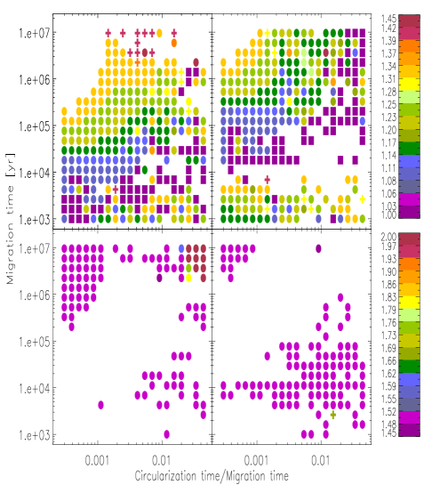
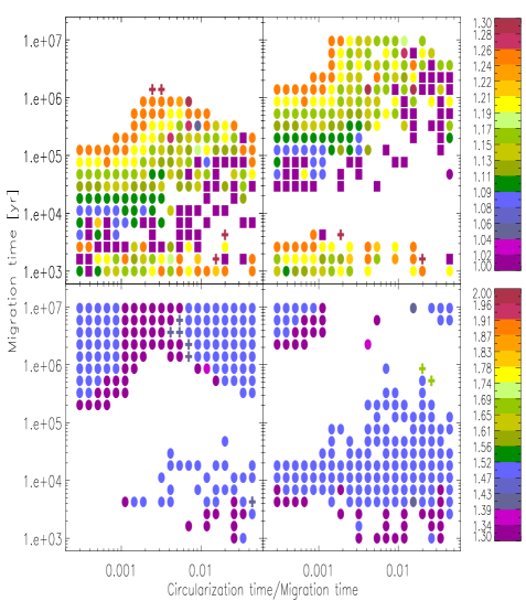
Figure 1: Final period ratios for planet pairs initialised on orbits close to 2:1 (left group of four panels) and 3:2 (right group of four panels) with the inner planet mass being $1\ {\rm M}_{\oplus}$ and the outer mass being $4\ {\rm M}_{\oplus}$. For each group of four panels, the upper and lower left panels give results for the outer planet starting at 1 AU and the upper and lower right panels give results for the outer planet starting at 5 AU. These respectively correspond to the surveys $1{\rm AU}\_1\_4\_21,\hskip 5.69054pt5{\rm AU}\_1\_4\_21,\hskip 5.69054pt1{\rm AU}\_1\_4\_32,$ and $\hskip 5.69054pt5{\rm AU}\_1\_4\_32.$ Period ratios are indicated in associated colour bars such that the larger values up to $2$ are indicated in the lower panels and the smaller values down to $1$ are indicated in the upper panels. Second order resonances are indicated by crosses (see text) and the purple squares indicate collisions between the planets. Note that in this and other similar figures, the migration time plotted is $\tau_{m0}$ and the ratio of circularization time to migration time plotted is $\tau_{c}/\tau_{mig}$ which are both independent of planet mass (see Equations (17)). For the simulations shown in the above panels the quantity, $1/(1/\tau_{mig,2}-1/\tau_{mig,1}),$ which estimates the initial convergence time for the outer and inner orbits is equal to $\tau_{m0}/3.$

3.2 Initial configuration

We considered planets with masses of either 1, 2 or 4 earth masses ($\mathrm{M}_{\oplus}$). The planets were initialised on circular coplanar orbits with the outer one being at 1 AU or 5 AU. The inner planet is initialised on an orbit which is exterior to either 2:1 or 3:2 mean motion resonance. The initial period ratio is $P_{1}/P_{2}=2.15$ in the former case and $P_{1}/P_{2}=1.7$ in the latter case. Note that the system is invariant to multiplying all lengths by a factor $f_{s}$ and times, including $\tau_{mig,i}$ and $\tau_{c,i},$ $i=1,2,$ by a factor $(f_{s})^{3/2}.$ These results can be extended to apply to cases with a different cavity radius.

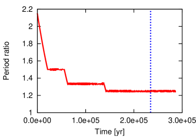
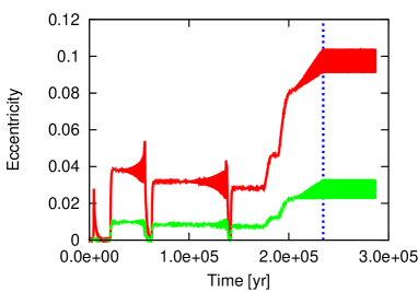
Figure 2: The evolution of the period ratio (left panel) and eccentricity (right panel) for a run contributing to the survey $1{\rm AU}\_1\_4\_21$ (see text). The vertical line in this and similar figures indicates the point at which both planets have entered the cavity.

4 Results

4.1 General features

In all the unextended surveys listed in Table 2, the outcome is that either the planets are in resonance or they collide. First and higher order resonances are possible but the latter are infrequent. We note that although planets attaining first order resonances may undergo an instability that causes the resonance to be broken (Goldreich & Schlichting, 2014), another resonance with smaller period ratio is quickly attained. Thus most of the time is spent in some resonance unless the migration is fast enough to cause the planets to collide.

All our runs are stopped at that point. To illustrate a typical case, we describe the evolution of the period ratio and eccentricity for a run taken from the survey, $1{\rm AU}\_1\_4\_21$, for which the complete set of results are illustrated in Fig. 1. The final period ratio is indicated in the eighth row and eighth column in the upper leftmost panel. The results are illustrated in Fig. 2. We recall that the outer planet mass was $4\ {\rm M}_{\oplus}$ and the inner planert mass $1\ {\rm M}_{\oplus}.$ Our migration prescription ensures convergent migration that first leads to trapping in the 3:2 resonance (e.g. Papaloizou & Szuszkiewicz, 2005). However, as the migration continues this is broken and a 4:3 resonance attained. That in turn is broken leading to a 5:4 resonance which remains until the pleanets both enter the cavity. Note that towards and until just before the end of the run, the eccentricities increase. This is a common feature of the runs presented here, being due to the loss of the damping effect of the circularization of the inner planet while it is temporarily driven inwards by the outer planet. Note that the transition from resonance to resonance seen here was also seen in simulations by Papaloizou & Szuszkiewicz (2009).

4.2 Results of the surveys with $(m_{1},m_{2})=(1,4)\ {\rm M}_{\oplus}$

In Fig. 1 the final period ratios for planet pairs initialised on orbits close to the 2:1 resonance are shown in the left set of four panels and close to the 3:2 resonance in the right set of four panels. For each set of four the upper and lower left panels give the result when the outer planet starts at 1 AU and the upper and lower right panels are for the outer planet starting at 5 AU. Apart from a few exceptions associated with the planets scattering as they enter the cavity, runs end with either the planets close to a resonance, or with a collision. Most of the resonances are first order and readily identified in Fig. 1 and similar figures below with the help of the colour bars (e.g. for surveys starting close to the 2:1 commensurability illustrated in Fig. 1, a filled dark red circle in the lower leftmost panels corresponds to 2:1 resonance, a filled purple circle in those two panels to the 3:2 resonance, a filled orange circle in the upper leftmost two panels to 4:3 resonance and a filled light green circle in the latter panels to 5:4 resonance).

In general planetary collisions are expected to occur for very fast migration (small migration time). However, the rate of migration required depends on the rate of orbital circularization, decreasing as the rate of circularization decreases. This is because weak circularization allows for the development of highly eccentric planetary orbits, making a collision through orbit crossing more probable. This trend can be seen in Figure 1 (and other surveys presented below). As migration times increase, collisions tend to require larger circularization times in order to occur. For example, from the left group of four panels in Fig. 1, we can quantify the migration and circularization time limits for collision. In the left panels with the outer planet starting at 1 AU, collisions can occur for $\tau_{c}/\tau_{mig}\leq 0.01$ provided that $\tau_{m0}\leq 10^{4}\ \mathrm{yr}.$ This corresponds to the quantity, $1/(1/\tau_{mig,2}-1/\tau_{mig,1})=\tau_{m0}/3,$ which estimates the convergence time through migration of the orbits of the outer and inner planets (see equations (12) and (17)), being $\leq 3\times 10^{3}\ \mathrm{yr}.$ However, when $\tau_{c}/\tau_{mig}\sim 0.1$, collision can occur for $\tau_{m0}\sim 10^{6}\ \mathrm{yr}$. Note that these times approximately increase by a factor $5^{3/2}$ for the right group of panels with the outer planet starting at 5 AU.

To decide whether a run ended with a relatively rare second order commensurability, we adopted the same criterion as above that fractional deviation from commensurability should be $\ <6\times 10^{-3}$. This was applied to all surveys. These were indicated in Fig. 1 and other similar figures by a cross. Thus for surveys with the outer planet starting close to the 2:1 resonance, a 5:3 resonance was indicated by an olive cross in the lower panel that is second from the left, a 7:5 resonance by a burgundy cross in the two upper leftmost panels and a 9:7 resonance by a yellow cross in the upper panel that is second from the left. These are discussed in more detail in Sections 4.4 and 4.4.1 below. The survey $1{\rm AU}\_1\_4\_21$ had also had runs that were associated with higher order resonances with period ratios close to 10:7, 8:5 and 11:6. These are discussed in more detail in Section 4.5.

4.3 Results of the surveys with $(m_{1},m_{2})=(1,2)\ {\rm M}_{\oplus}$ and $(m_{1},m_{2})=(2,1)\ {\rm M}_{\oplus}$

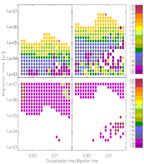
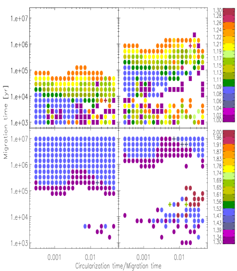
Figure 3: Final period ratios for planet pairs initialised on orbits close to 2:1 (left group of four panels) and 3:2 (right group of four panels) with the inner planet mass being 1 ${\rm M}_{\oplus}$ and the outer mass being 2 ${\rm M}_{\oplus}$. For each group of four panels, the upper and lower left panels give results for the outer planet starting at 1 AU and the upper and lower right panels give results for the outer planet starting at 5 AU. These respectively correspond to the surveys $1{\rm AU}\_1\_2\_21,\hskip 5.69054pt5{\rm AU}\_1\_2\_21,\hskip 5.69054pt1{\rm AU}\_1\_2\_32,$ and $\hskip 5.69054pt5{\rm AU}\_1\_2\_32.$ Period ratios are indicated in the associated colour bars such that the larger values up to $2$ are indicated in the lower panels and the smaller values down to $1$ are indicated in the upper panels. Second order resonances are indicated by crosses (see text) and the purple squares indicate collisions between the planets. For these cases, the quantity $1/(1/\tau_{mig,2}-1/\tau_{mig,1}),$ which estimates the initial convergence time for the outer and inner orbits is $\tau_{m0},$ which is the migration time plotted.

These surveys are carried out and the results are presented in the same manner as the surveys with $(m_{1},m_{2})=(1,4)\ {\rm M}_{\oplus},$ the only change being that they are carried out with different planet masses. The qualitative description of the results is found to be the same.

The results for the surveys with $(m_{1},m_{2})=(1,2)\ {\rm M}_{\oplus}$ are shown in Fig. 3.

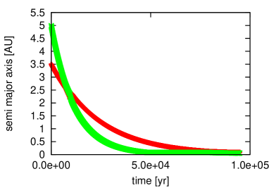
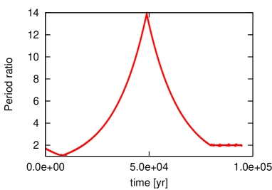
Figure 4: The evolution of the period ratio (left panel) and eccentricity (right panel) for a run contributing to the survey $5{\rm AU}\_1\_2\_32$(see text). In this case the planets undergo orbit crossing and scatter causing the inner and outer planets to be interchanged.

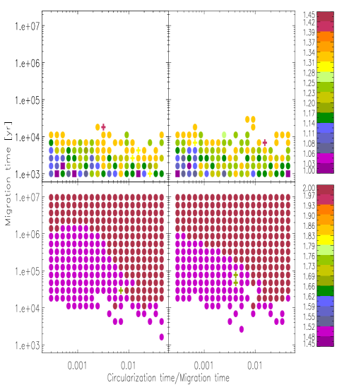
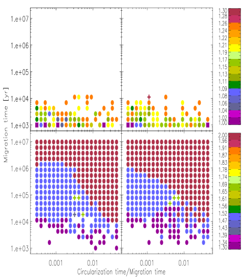
Figure 5: Final period ratios for planet pairs initialised on orbits close to 2:1 (left group of four panels) and 3:2 (right group of four panels) with the inner planet mass being 2 ${\rm M}_{\oplus}$ and the outer mass being 1 ${\rm M}_{\oplus}$. For each group of four panels, the upper and lower left panels give results for the outer planet starting at 1 AU and the upper and lower right panels give results for the outer planet starting at 5 AU. These respectively correspond to the surveys $1{\rm AU}\_2\_1\_21,\hskip 5.69054pt5{\rm AU}\_2\_1\_21,\hskip 5.69054pt1{\rm AU}\_2\_1\_32,$ and $\hskip 5.69054pt5{\rm AU}\_2\_1\_32.$ Period ratios are indicated in associated colour bars such that the larger values up to $2$ are indicated in the lower panels and the smaller values down to $1$ are indicated in the upper panels. Second order resonances are indicated by crosses (see text) and the purple squares indicate collisions between the planets. The quantity $1/(1/\tau_{mig,1}-1/\tau_{mig,2}),$ which for these cases estimates the initial divergence time for the outer and inner orbits is $\tau_{m0},$ which is the migration time plotted.

These surveys produce a similar number of collisions, range of first order resonances and second order resonances as the previous ones. However, they differ in that a significant number of 2:1 commensurabilites are formed at high migration rates and relatively low circularization rates. These are seen in the second and fourth of the lower panels counted from the left of Fig. 3. They are found to be associated with a scattering and interchange of the planets. Figure 4 shows the evolution for a run taken from the survey $5{\rm AU}\_1\_2\_32.$ It is indicated in the ninth row from bottom and rightmost column of the rightmost lower panel of Fig. 3. In this run the planets undergo orbit crossing and scatter causing the inner and outer planets to be interchanged and a large period ratio $\sim 14$ attained. Subsequently convergent migration resumes and a 2:1 commensurability is formed.

Results for the surveys with $(m_{1},m_{2})=(2,1)\ \mathrm{M}_{\oplus}$ are shown in Fig. 5. In this case the general form of the orbital evolution differs from the previous cases. As the inner planet is more massive than the outer planet, the initial inward migration is divergent. Only when the inner planet has reached the inner cavity while the outer planet is still migrating can their semi-major axes start to approach each other and their period ratio starts to decrease so that a resonance can form. The nature of this evolution allows a significantly larger number of 2:1 comensurabilities to result from systems with larger migration rates, as compared to the previous surveys.

Note that the simulations with the outer planet starting at 5 AU, would lead to the same results as in the case of the outer planet starting at 1 AU if the timescales were multiplied by a factor of $5^{3/2}$ and the inner cavity radius was also increased by a factor of five. However, because the inner cavity radius is in fact the same in both cases, the simulations with the outer planet starting at 5 AU map into simulations starting at 1 AU with a reduced inner cavity radius. This results in a simulation that is allowed to evolve for longer. This has the consequence that the planets end up closer together or with smaller period ratios than would occur if the simple scaling was assumed. This is apparent for example when the left and right panels in the leftmost group of four panels in Fig. 5 are compared. However, the simple scaling is relatively more closely adhered to when collisions are considered because the inner cavity plays less of a role in those cases (see discussion of the results shown in Figs 1 in section 4.2 ).

In Figure 6 we show the orbital evolution of a run taken from the survey $1{\rm AU}\_2\_1\_32.$ It corresponds to the run indicated in the eleventh row (from bottom) and eleventh column (from left) of the third lower panel from the left in Fig. 5. During the first part of the simulation, the inner planet migrates much faster inwards than the outer planet leading to a significant increase of their period ratio. This growth suddenly comes to a stop when the inner planet has reached the cavity and its migration switches off. From this time on, the period ratio decreases until a persisting 3:2 mean-motion resonance forms.

In addition to producing more 2:1 commensurabilities significantly fewer collisions were found in these surveys as compared to the previously discussed ones. However, a comparable number of second order resonances were found.

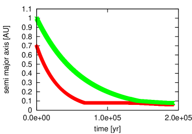
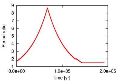
Figure 6: Evolution of the semi-major axis and the period ratio for a run taken from the survey $1{\rm AU}\_2\_1\_32$ for which the inner planet is more massive (see text).

4.4 Occurence of second-order resonances

In Table 2 we show the number of second-order resonances found in all of the surveys discussed above. We detected 5:3, 7:5 and 9:7 resonances. These are indicated in the figures illustrating the final period ratios.

From Table 2, there were $72$ occurrences out of a total of $4800$ simulations giving an incidence rate of $1.5\%.$ Although, these occurrences are rare, as they may contain useful information concerning their origin, we now examine some of them in more detail.

4.4.1 Detailed study of second-order resonances

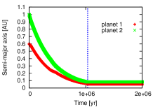
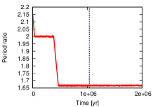
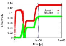
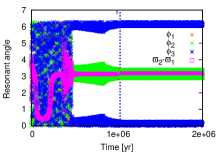
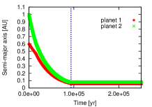
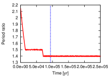
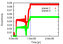
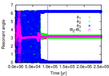
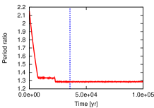
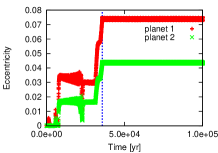
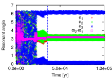
Figure 7: Semi-major axis (first column), period ratio (second column), eccentricity (third column) and resonant angles $\phi_{1}$, $\phi_{2}$ and $\phi_{3}$ as well as $\varpi_{2}-\varpi_{1}$ (fourth column) for runs that attained the commensurabilities 5:3 (upper panels), 7:5 (middle) and 9:7 (lower panels). The point at which both planets have entered the inner cavity is indicated by the vertical line.

Resonance	$e_{1}$	$e_{2}/e_{1}$	$r$
5:3	0.13	0.65	0.571
	0.07	0.571	0.557
7:5	0.087	0.575	0.504
9:7	0.075	0.560	0.456
	0.03	0.5	0.481

Table 3: Comparison of numerical (third column ) and semi-analytically determined (fourth column) eccentricity ratios. The resonance and value of the eccentricity of the inner planet are indicated in the first and second column, respectively.

We now examine some runs which ended with the planets in a second order resonance in more detail. For these the inner planet mass was 1 $\mathrm{M}_{\oplus}$ and the outer planet mass was 2 ${\rm M}_{\oplus}$. The outer planet started at 1 AU just outside the 2:1 resonance with the inner planet. They form part of the survey $1{\rm AU}\_1\_2\_21$ for which results are illustrated in the panels furthest to the left of Fig. 3. We consider the unique runs in this survey that ended with the planets in 7:5 and 9:7 resonances and the run corresponding to the second to last entry in the fifth row from the top of the lower panel furthest to the left. The latter (case A) is one of several that ended in 5:3 resonance. It had $\tau_{mig}=1.5\times 10^{6}(\mathrm{M}_{\oplus}/m_{i})\ {\rm yr}$ and $\tau_{c}/\tau_{mig}=0.03.$ For the 7:5 resonance case (case B), $\tau_{mig}=1.2\times 10^{5}(\mathrm{M}_{\oplus}/m_{i}))\ {\rm yr}$ and $\tau_{c}/\tau_{mig}=0.015$ and for the 9:7 case (case C) $\tau_{mig}=5\times 10^{4}(\mathrm{M}_{\oplus}/m_{i}))\ {\rm yr}$ and $\tau_{c}/\tau_{mig}=0.012.$

The evolution of the semi-major axes, period ratios, eccentricities and resonant angles for these cases is illustrated in Fig. 7. At early times a first order resonance is attained, 2:1 in case A, 3:2 in case B and 4:3 in case C. This becomes unstable and the second order resonance is entered and maintained until the end of the run. $\phi_{1}$, $\phi_{2}$ and $\phi_{3}$ are the resonant angles as defined in Eqs. (3) - (4). For all three simulations, when the second-order resonance occurs, $\phi_{1}$ and $\phi_{2}$ are around $\pi$ while $\phi_{3}$ is librating around 0 and $2\pi$. We recall that $\varpi_{2}-\varpi_{1}$ is the angle between the apsidal lines which is found to librate around $\pi$.

Averaging out short period oscillations, constant equilibrium eccentricities, as indicated in Section 2.4 are attained, though this phase is short lived in case B. The eccentricties start to jump just after the inner planet starts to enter the cavity. This is because when it no longer intersects the disc, migration and circularization then only operate on the outer planet, At later times, final constant values of the eccentricities are attained that are larger than those applying when both planets were affected by migration and circularization.

We have tested the applicability of Equation (13 ) for the eccentricity ratio and Equation (12) which, with the help of Appendix A, enables the calculation of the magnitues of the eccentricities during phases when the system undergoes self-similar migration, which we here identify with the phases when the eccentricities are approximately constant with superposed small amplitude short period oscillations. Equation (12) then enables the calculation of the eccentricities as a function of the migration and circularization times. In addition comparison of the numerically determined eccentricity ratios with those obtained from the semi-analytic procedure is given in Table 3. It is seen that there is good agreement, especially for the smaller eccentricties. In these cases adequate calculations can be performed taking only second order terms into account (see Appendix A). The absolute values of the eccentrities are also found to agree with those implied by (12).

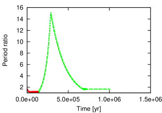
Figure 8: The period ratio evolution for the run taken from $5{\rm AU}\_1\_4\_32$ that shows a scattering followed by the attainment of a 5:3 resonance (see text).

In Fig. 1 there are two green crosses corresponding to 5:3 resonances that can be seen in in the rightmost lower panel showing the survey with the outer planet starting at 5 AU. In these cases the relatively rapid convergent migration rates result in orbit crossing leading to the planets changing places. The original inner planet is scattered outwards such that the system attains large period ratios $>14.$ Convergent migration resumes after the now more massive inner planet enters the cavity resulting in the attainment of a 5:3 resonance. The period ratio as a function of time for the case with the shortest migration time is shown in Fig. 8.

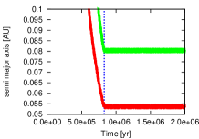
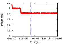
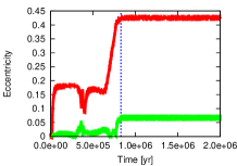
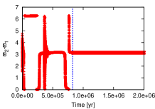
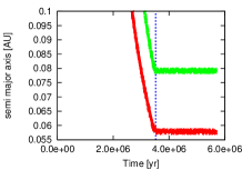
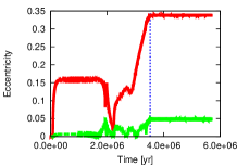
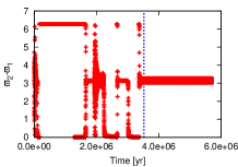
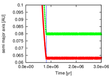
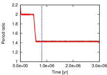
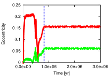
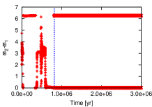
Figure 9: Semi-major axis (first column), period ratio (second column), eccentricity (third column) and the angle between the apsidal lines $\varpi_{2}-\varphi_{1}$ (fourth column) for runs with ultimate period ratios near 1.83 (upper panels), 1.6 (middle panels) and 1.427 (lower panels) that were carried out in the survey $1{\rm AU}\_1\_4\_21.$

4.5 Runs indicating higher order resonances

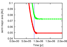
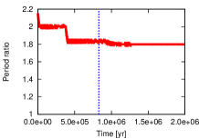
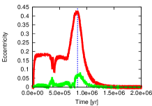
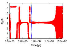
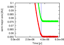
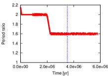
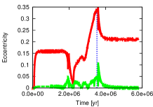
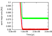
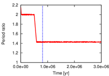
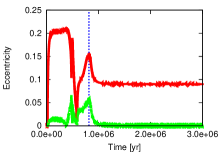
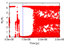
Figure 10: As in Fig. 9 but in this case after point where both planets enter the cavity, the runs are extended with migration forces switched off while circularization forces continue to act only on the outer planet.

To illustrate the potential presence of higher order resonances we illustrate the evolution of runs taken from the survey $1{\rm AU}\_1\_4\_21.$ These were cases with final period ratios 1.83 (case D), 1.6 (case E) and 1.427 (case F). Case D corresponds to the run shown in the fourth row (from top) and third column from the end in the lower leftmost panel of Fig. 1. Case E corresponds to the run shown in the top row and fourth column from the end in the lower leftmost panel of Fig. 1. Case F corresponds to the run shown in the fourth row and second column from the end in the upper leftmost panel of Fig. 1. The time independent evolution of the semi-major axes, eccentricities and angle between the apsidal lines for these cases is illustrated in Fig. 9. Each of these runs initially attains a 2:1 resonance which is not sustained (Goldreich & Schlichting, 2014). The systems leave it and attain period ratios close to 11:6, 8:5 and 10:7 in cases D, E and F respectively. The angle between the apsidal lines oscillates between $0$ and $\pi$ before settling on $\pi$ in cases D and E and $0$ in case F after the planets have entered the cavity and forces arising from migration and circularization were removed. Note that the eccentricities are large in these runs attaining $\sim 0.45$ in case D.

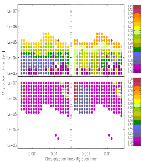
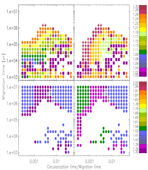
Figure 11: Final period ratios after extended runs for planet pairs initialised on orbits close to 2:1 (left hand set of four panels) and 3:2 (right hand set of four panels) are shown in the upper and lower right hand panels of each group of four. The upper and lower left hand panels for each set show the period ratios at the commencement of the extension of the runs ( the result of the unextended surveys $1{\rm AU}\_1\_2\_21$ and $1{\rm AU}\_1\_4\_32$) for comparison. The inner planet mass is 1 $\mathrm{M}_{\oplus}$ and the outer mass 2 $\mathrm{M}_{\oplus}$ in the first case and 4 $\mathrm{M}_{\oplus}$ in the second. The outer planet starts at 1 AU for all runs. The purple squares again show simulations with collisions between the planets.

To investigate the subsequent evolution of the period ratios that could occur if additional dissipative forces were imposed we performed an additional set of runs for which circularization was allowed to continue to operate on the outer planet after the cavity was entered, The evolution of these runs is illustrated in Fig. 10. It will be seen that the eccentricities decrease while changes to the period ratio are on average very small. The inner planet has the larger eccentricity while dissipation occurs only for the outer planet. The eccentricity of the inner planet decreases through secular transfer to the outer planet which is indicated by maintenance of the angle between the apsidal lines at $0$ or $\pi.$ In case D the latter fails once both eccentricities become very small and the angle loses its significance. In all cases the evolution ceases as the eccentricity of the outer planet approaches zero. During the later stages of evolution, energy is removed from the orbit of the outer planet, but not that of the inner planet, causing the period ratio to decrease very slightly.

4.6 Continuation of runs with orbital circularization but with no migration torques

In this section, we describe some surveys of the second type that were continued after the planets have reached the inner cavity. We begin by considering extensions of the surveys $1{\rm AU}\_1\_2\_21$ and $1{\rm AU}\_1\_4\_32$ the results of which are shown in Figs 3 and 1.

For the extensions to the runs, as described above we allow circularization to continue only for the outer planet while migration is deactivated for both planets interior to the cavity. Each run was then continued for a time which is the shorter of either $5\times t_{max}$ or $2\times 10^{7}\ \mathrm{yr},$ with $t_{max}$ being the duration of the unextended run.

Figure 11 shows the final period ratio at start of this continuation on the left panel and the final period ratio after continuing the simulations. By making a comparison one can see that the period ratios are increased. This is expected because during this evolution, the planetary systems have energy removed at constant angular momentum, and the theoretical expectation is that they should separate with period ratio increasing as a function of time (e.g. Papaloizou, 2011).

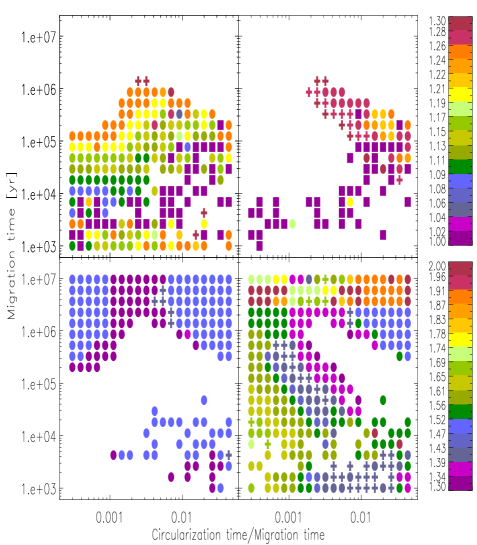
Figure 12: Final period ratios after the runs in the survey extended from $1{\rm AU}\_1\_4\_32$ that are shown in Fig. 11 were further extended for an additional time, $0.1t_{max},$ with a circularization time of $20$ orbits for both planets, are shown in the right hand panels. The upper and lower left hand panels show the period ratios at the commencement of the first extension of the runs (the result of the unextended survey $1{\rm AU}\_1\_4\_32$). The purple squares show simulations with collisions between the planets.

This is especially the case for small values of the ratio of the circularization time to the migration time (see the left hand sides of the panels). For example inspection of the two lower leftmost panels of Fig. 11 shows systems that were in 3:2 resonance increasing their period ratios in to the 1.52 - 1.56 domain for both surveys illustrated. However, changes are much smaller for longer circularization times. In addition the period ratio range $1.7-1.8$ is empty. This can be rectified if shorter circularization times are used so inducing a more rapid separation of the planetary systems. We note the phenomenon of wake-planet interaction discussed by Baruteau & Papaloizou (2013) that could lead to the same effect and was modelled through the introduction of orbital circularization.

To illustrate how the results depend on the amount of circularization (or wake-planet interaction) introduced we have perfomed a simplified illustrative calculation by extending the continuation of $1{\rm AU}\_1\_4\_32$ described above such that each run is extended for a further $0.1t_{max},$ where $t_{max}$ is the duration of the run in the unextended survey, during which the circularization time for each planet taken to be $20$ orbits, as was adopted in Baruteau & Papaloizou (2013). Results are shown in Fig. 12. It will be seen that period ratios throughout the range $1.7-2$ are obtained.

The criteria for a run to have terminated in a second order resonance were applied in the same way as for the other surveys and more are found after this doubly extended survey completes. However, as in this case they are formed from divergent migration, capture into libration is not expected. This is indeed found to be the case. Thus runs of the type illustrated in Fig. 7, which end with resonant angles librating, do not occur when the near second order commensurabilities are obtained as a result of divergent migration produced through the action of efficient orbital circularization.

5 Summary and conclusions

In order to investigate the possible consequences for potential architectures of low mass planetary systems, we have performed numerical simulations of a pair of coplanar migrating low-mass planets in the mass range $(1-4)\ \mathrm{M}_{\oplus}.$ In the surveys we conducted, the planets were initialised on circular coplanar orbits with the outer one being at 1 AU or 5 AU. Outside an inner cavity of radius $0.08\ {\rm AU}$, the orbital evolution was considered for a constant migration time, $\tau_{mig},$ in the range $(10^{3}-10^{7})(M_{\oplus}/m_{i})\ \mathrm{yr}$ and constant ratio of circularization time to migration time $\tau_{c}/\tau_{mig}$ in the range $3\times 10^{-4}-4.4\times 10^{-2}$. These could be viewed as possibly arising from interaction with a protoplanetary disc. The inner planet was initialised on an orbit which was close to and exterior to either the 2:1 or the 3:2 mean motion resonance. Note that the length and time scales we used can be scaled to other values using the standard scalings for systems governed by gravity (see Section 3.2).

In order to provide a simple model of phenomena producing an inner cavity boundary to a protoplanetary disc, such as rapid changes in disc viscosity or interaction with the stellar magnetic field, we considered migration to terminate inside the cavity but performed some extended surveys for which circularization was allowed to continue for one or both planets. We remark that the latter set up could be viewed as providing a heuristic modelling of phenomena such as wake-planet interactions, or planet-density wave interactions (e.g. Baruteau & Papaloizou, 2013) or even residual planetesimal migration (e.g. Minton & Levison, 2014) that can halt or turn around convergent migration of the planets. We remark that the work here is carried out in order to characterise the possible outcomes for migrating two planet systems under very simple assumptions about forces leading to migration and circularization. It does not constitute population synthesis studies.

Numerical simulations that terminated without an extended period of circularization resulted for the most part in, either collisions between the planets or, the formation of systems close to resonance. These were mostly first order with second order resonances occurring in a few $\%$ of cases. Those were found to occur for modest eccentricities $<\sim 0.1$ and all resonant angles librated (see Section 4.4.1). This is in contrast to the situation where the near commensurability resulted from divergent migration of the type encountered in the extended surveys. In those cases resonant trapping does not occur and the resonant angles circulate. Thus the behaviour of the resonant angles in systems near a second order commensurability can indicate the form of any migration that led to them.

An analytic description of planets migrating in second order resonances was given in Sections 2 - 2.6. There we derived expressions for the ratio of the eccentricities of the planets and the absolute values of the eccentricities as a function of the ratio of circularization time to migration time. The ratio of the eccentricities was subsequently evaluated correctly to fourth order in the eccentricities for several cases and was found to be in reasonable agreement with simulations. In a very small number of cases, period ratios corresponding to even higher order resonances were seen. These were discussed in Sections 2.7 and 4.5.

In order to obtain an extended range of final period ratios, it was necessary to extend the simulations so that the planet(s) underwent a period of circularization without migration. The important consequence of this is that there is a period of effective divergent migration that causes the period ratios to diverge. Depending on its effectiveness, the whole range of period ratios in $(1,2)$ could be obtained (see Section 4.6). Thus, in order to determine final outcomes of planetary systems, the study of their interaction with the inner parts of a protoplanetary disc is crucial. A better understanding of the detailed inner disc structure, the effects of any density waves launched by an interaction with the central star and the interaction of any residual planetesimal disc will be required. These issues will form the focus of future studies.

Appendix A The direct part of the disturbing function for second order resonances

In order to discuss the $(p+2):p$ resonance, the quantity $R_{D}$ is written in the compact general form

$$R_{D}=\sum_{n,i}F_{i}^{n}\cos(n\theta_{j}-i\varpi_{1}+(i-2n)\varpi_{2}),$$ (18)

where $\theta_{j}=(p+2)\lambda_{2}-p\lambda_{1}.$ Here the index of summation $n$ is a non negative integer and the index of summation, $i,$ is a positive or negative integer or zero. In addition terms that turn out to have the same cosine factor are collected together in the expressions given below. We take into account terms up to fourth order in the eccentricity such that $R_{D}$ takes the explicit form

$$R_{D}=F_{0}^{0}+F_{1}^{0}\cos(\varpi_{2}-\varpi_{1})+F_{2}^{0}\cos 2(\varpi_{2}-\varpi_{1})+$$

$$F_{2}^{1}\cos(\theta_{j}-2\varpi_{1})+F_{1}^{1}\cos(\theta_{j}-\varpi_{2}-\varpi_{1})+$$

$$F_{0}^{1}\cos(\theta_{j}-2\varpi_{2})+F_{3}^{1}\cos(\theta_{j}+\varpi_{2}-3\varpi_{1})+$$

$$F_{-1}^{1}\cos(\theta_{j}+\varpi_{1}-3\varpi_{2})+F_{4}^{2}\cos(2\theta_{j}-4\varpi_{1})+$$

$$F_{3}^{2}\cos(2\theta_{j}-3\varpi_{1}-\varpi_{2})+F_{2}^{2}\cos(2\theta_{j}-2\varpi_{1}-2\varpi_{2})+$$

$$F_{1}^{2}\cos(2\theta_{j}-\varpi_{1}-3\varpi_{2})+F_{0}^{2}\cos(2\theta_{j}-4\varpi_{2})\ ,$$ (19)

where

$$F_{0}^{0}=f_{0}+(e^{2}_{1}+e^{2}_{2})f_{2}+e_{1}^{4}f_{4}+e_{1}^{2}e_{2}^{2}f_{5}+e_{2}^{4}f_{6}$$

$$F_{1}^{0}=e_{1}e_{2}f_{10}+e^{3}_{1}e_{2}f_{11}+e_{1}e_{2}^{3}f_{12}$$

$$F_{2}^{0}=e_{1}^{2}e^{2}_{2}f_{17}$$

$$F_{2}^{1}=e^{2}_{1}f_{45}+e^{2}_{1}e^{2}_{2}f_{47}+e_{1}^{4}f_{46}$$

$$F_{1}^{1}=e_{1}e_{2}f_{49}+e_{1}^{3}e_{2}f_{50}+e_{1}e_{2}^{3}f_{51}$$

$$F_{0}^{1}=e_{2}^{2}f_{53}+e_{1}^{2}e_{2}^{2}f_{54}+e_{2}^{4}f_{55}$$

$$F_{3}^{1}=e_{1}^{3}e_{2}f_{68}$$

$$F_{-1}^{1}=e_{2}^{3}e_{1}f_{69}$$

$$F_{4}^{2}=e^{4}_{1}f_{90}$$

$$F_{3}^{2}=e^{3}_{1}e_{2}f_{91}$$

$$F_{2}^{2}=e^{2}_{1}e_{2}^{2}f_{92}$$

$$F_{1}^{2}=e_{1}e_{2}^{3}f_{93}$$

$$F_{0}^{2}=e_{2}^{4}f_{94}.$$ (20)

the quantities $f_{i}$ and $f_{ij}$ are functions only of $\alpha=a_{1}/a_{2}$ and their forms are tabulated in Appendix B of Murray & Dermott (1999).

References

- Baruteau & Papaloizou (2013) Baruteau, C., Papaloizou J.C.B., 2013, ApJ, 778, 7
- Batalha et al (2013) Batalha, N. M., Rowe, J. F., Bryson, S. T., et al., 2013, ApJS, 204, 24
- Goldreich & Schlichting (2014) Goldreich P. & Schlichting H. E., 2014, AJ, 147, 32
- Kley et al. (2004) Kley W., Peitz J., Bryden G., 2004, A&A, 414, 735
- Izidoro et al. (2014) Izidoro, A., Morbidelli, A., Raymond, S. N., ApJ., 794, 11
- Jenkins et al. (2013) Jenkins, J. S., Tuomi, M., Brasser, R., Ivanyuk, O., Murgas, F. , 2013, ApJ, 771, 41
- Jenkins & Tuomi (2014) Jenkins, J. S. & Tuomi, M., 2014, ApJ, 794, 110
- Lissauer et al. (2012) Lissauer, J. J., Marcy, G. W., Rowe, J. F., et al., 2012, ApJ, 750, 112
- Lee & Peale (2002) Lee, M.H., Peale S.J., 2002, ApJ, 567, 596
- Minton & Levison (2014) Minton D. A.,& Levison, H.F., 2014, Icarus, 232,118
- Murray & Dermott (1999) Murray, C.D., & Dermott, S. F., 1999, Solar System Dynamics, Cambridge Univ. Press, Cambridge
- Nelson & Papaloizou (2002) Nelson R. P. & Papaloizou J.C.B., 2002, MNRAS, 333, 26
- Papaloizou (2003) Papaloizou J.C.B., 2003, Cel. Mech. and Dynam. Astron., 87, 53
- Papaloizou (2011) Papaloizou J.C.B., 2011, Cel. Mech. and Dynam. Astron., 111, 83
- Paardekooper et al. (2010) Paardekooper, S.-J., Baruteau, C., Crida, A., Kley, W., 2010, MNRAS, 401,1950
- Papaloizou & Larwood (2000) Papaloizou J.C.B. & Larwood J.D., 2000, MNRAS, 315, 823
- Papaloizou & Szuszkiewicz (2005) Papaloizou J.C.B. & Szuszkiewicz, E., 2005, MNRAS, 363, 153
- Papaloizou & Szuszkiewicz (2009) Papaloizou J.C.B. & Szuszkiewicz, E., 2009, EAS, 42, 333
- Papaloizou & Terquem (2010) Papaloizou J.C.B. & Terquem, C., 2010, MNRAS, 405, 573
- Rein & Liu (2012) Rein H. & Liu S.-F., 2012, A&A, 537, A128
- Snellgrove et al. (2001) Snellgrove, M. D., Papaloizou, J. C. B., Nelson, R. P., 2001, A&A, 374,10029
- Steffen (2013) Steffen, J. H., 2013, MNRAS, 433, 32465