Nonlinear acoustic wave generation in a three-phase seabed

Abstract

Generation of an acoustic wave by two pump sound waves is studied in a three-phase marine sediment that consists of a solid frame and the pore water with air bubbles in it. To avoid shock-wave formation the interaction is considered in the frequency range where there is a significant amount of sound velocity dispersion. Nonlinear equations are obtained to describe the interaction of acoustic waves in the presence of air bubbles. An expression for the amplitude of the generated wave is obtained and numerical analysis of its dependence on distance and on the resonance frequency of bubbles is performed.

I Introduction

Marine sediments as porous media consisting of a solid frame and the pore water are known to exhibit strong elastic nonlinearity hov ; bel ; z1 ; z2 . In the present paper nonlinear sound wave generation by two pump acoustic waves is studied in a three-phase marine sediment, that is in a sediment that contains air bubbles in its liquid fraction. Nonlinear oscillations of gas bubbles in fluids lead to considerable enhancement of the nonlinearity of a homogeneous medium za ; wel ; zab ; wu as well as of the nonlinear properties of marine sediments that contain bubbles in the pore water don ; ch . In Ref. 2012 nonlinear interaction of three sound waves was studied in a two-phase marine sediment without air bubbles in the liquid phase. In the present paper the sound wave generation in a three-phase sediment is considered, as in Ref. 2012 , in the frequency range where there is a significant amount of wave velocity dispersion tur ; sto ; isak ; buch . Due to velocity dispersion no shock-wave formation would occur which allows observing more explicitly interaction of three waves propagating in three different directions.

II Theory

Our task is to find the amplitude of an acoustic wave $(\omega_{3},{\bf k}_{3})$ generated by two pump acoustic waves $(\omega_{1},{\bf k}_{1})$ and $(\omega_{2},{\bf k}_{2})$, the nonlinearity being due to oscillating bubbles. The frequencies and wave vectors satisfy the energy and momentum conservation laws,

$$\omega_{1}+\omega_{2}=\omega_{3},\qquad{\bf k}_{1}+{\bf k}_{2}={\bf k}_{3}.$$

The dependence of the wave $(\omega_{3},{\bf k}_{3})$ amplitude on the resonance bubble frequency and on distance will be analyzed along with the possibility of experimental observation of the process.

To solve the problem we are based on the well-known Biot model in the form of the equations of continuity and momentum conservation for the liquid and solid fractions nik ,

$$\frac{\partial\rho_{m}}{\partial t}+\rho_{0m}\frac{\partial v}{\partial x}=0,\,\,\,\,\,\,\,\,\,\rho_{0m}\frac{\partial v}{\partial t}=-\frac{\partial p}{\partial x},$$

$$\frac{\partial\rho_{s}}{\partial t}+\rho_{0s}\frac{\partial u}{\partial x}=0,\,\,\,\,\,\,\,\,\,(1-m)\rho_{0s}\frac{\partial u}{\partial t}=\frac{\partial\sigma_{xx}}{\partial x}-(1-m)\frac{\partial p}{\partial x}$$ (1)

In these equations we can limit ourselves for simplicity with one-dimensional case since the angles between the three waves are small enough. Indeed, numerical estimates 2012 show that for the experimental situation which is used here and which is described in Refs. tur ; buch the angles between the propagation directions of the waves $(\omega_{1},{\bf k}_{1}),(\omega_{2},{\bf k}_{2})$ and the propagation direction (let it be the $x$-axis) of the wave $(\omega_{3},{\bf k}_{3})$ are approximately $\theta_{1}\approx 25^{\circ}$ and $\theta_{2}\approx 18^{\circ}.$

In Eqs. (1) nonlinear hydrodynamic terms are omitted since as it was noted in Introduction nonlinear acoustic processes are governed mainly by nonlinear oscillations of bubbles contained in the pore water. In Eqs. (1) $\rho_{m}$ is the mean density of the mixture of water and air bubbles; $\rho_{s}$ is the solid phase density, (the subscript ”0” refers to the equilibrium values); $v$ and $u$ are the velocities of the liquid and solid phases; $p$ is the pressure in the water; $m$ is the porosity; $\sigma_{xx}$ denotes the effective stress in a porous medium (see nik ),

$$\sigma_{xx}=-\left[k+(4/3)\mu\right]\frac{\delta\rho_{s}}{\rho_{0s}}+\frac{k}{k_{s}}p,$$

$k$ and $\mu$ are the bulk and shear moduli of the frame of the porous medium.

Further calculations performed by one of the authors in Ref. eng lead to the equations

$$\frac{\partial^{2}p}{\partial t^{2}}-\frac{m}{\rho_{0f}G}\frac{\partial^{2}p}{\partial x^{2}}-\frac{\nu}{\rho_{0s}G}\frac{\partial^{2}\rho_{s}}{\partial t^{2}}=\frac{mn}{G}\frac{\partial^{2}V}{\partial t^{2}}$$

$$\frac{\partial^{2}\rho_{s}}{\partial t^{2}}(1-m)-\frac{k+(4/3)\mu}{\rho_{0s}}\frac{\partial^{2}\rho_{s}}{\partial x^{2}}-\nu\frac{\partial^{2}p}{\partial x^{2}}=0$$ (2)

Here $n$ is the bubble concentration and $V$ is the bubble volume. Eqs. (2) should be supplemented with the equation for the individual bubble motion zab ,

$$\ddot{V}+\omega_{0}^{2}V+f\dot{V}-\alpha V^{2}-\beta(2\ddot{V}V+\dot{V}^{2})=\epsilon p,$$ (3)

where $\omega_{0}$ is the resonance bubble frequency. The coefficients in Eq. (3) are expressed through the equilibrium bubble volume $V_{0}$, its radius $R_{0}$ and the adiabatic index $\gamma$,

$$\alpha=\omega_{0}^{2}(1+\gamma)/2V_{0},\,\,\,\,\,\,\,\beta=1/6V_{0},\,\,\,\,\,\,\epsilon=4\pi R_{0}/\rho_{0f},\,\,\,\,\,\,\,f=\delta\omega_{0},$$

$\delta$ is the dimensionless absorption coefficient of bubble oscillations.

As was mentioned in Introduction in order to observe three-wave interaction in a more explicit way we should use the frequency range with a noticeable velocity dispersion. It is preferable to choose the interval of the maximum velocity dispersion to ensure that the angles between the waves are not too small, otherwise they would fall in the dissipation spreading of the waves. As in Ref. 2012 , the data from tur listed in Fig. 2 of buch will be used. Basing on these data we choose the frequencies equal to $\omega_{1}=2\pi\cdot 2\cdot 10^{3}\,{\rm s}^{-1}$, $\omega_{2}=2\pi\cdot 3\cdot 10^{3}\,{\rm s}^{-1}$, for which the sum frequency equals   $2\pi\cdot 5\cdot 10^{3}\,{\rm s}^{-1}$. We shall seek for the solution to Eqs. (2), (3) in the form

$$p_{i}=1/2[P_{i}e^{i(k_{i}x-\omega_{i}t)}+{\rm c.c.}],\,\,\,\,\,\,\,\,\,\,V_{i}=1/2[V_{i}e^{i(k_{i}x-\omega_{i}t)}+{\rm c.c.}],\,\,\,\,\,\,i=1,2,3.$$

The only nonlinear term in Eqs. (2) that ensures the nonlinear process is the last term of the first equation. In fact this term is the sum of the linear $V^{l}$ and the nonlinear part $V^{n}$. The nonlinear part $V^{n}$ responsible for the generation of the wave $p_{3}$ by the waves $p_{1}$, $p_{2}$ can be obtained from Eq. (3) in the form

$$V^{n}=\frac{[\alpha-\beta(\omega_{1}^{2}+\omega_{2}^{2}+\omega_{1}\omega_{2})]\epsilon^{2}p_{1}p_{2}}{(-\omega_{3}^{2}+\omega_{0}^{2}-i\omega_{3}f)(\omega_{1}^{2}-\omega_{0}^{2}+i\omega_{1}f)(\omega_{2}^{2}-\omega_{0}^{2}+i\omega_{2}f)}.$$ (4)

In solving the equations (2) the so called approximation of a fixed field is used, that is the changes of the amplitudes $P_{1}$, $P_{2}$ because of nonlinearity are neglected, their changes being only due to linear bubble oscillations that cause dispersion in the medium. Using (4) we obtain the solution to Eqs. (2) for the amplitudes $P_{1},P_{2},P_{3}$ that are assumed to vary slowly at the distance of order of the wave length,

$$\frac{dP_{1}}{dx}=ib_{1}P_{1},\,\,\,\,\,\,\,\,\,\frac{dP_{2}}{dx}=ib_{2}P_{2},\,\,\,\,\,\,\,\,\,\frac{dP_{3}}{dx}=ib_{3}P_{3}-iaP_{1}P_{2}.$$ (5)

The following notations are used in Eqs. (5),

$$b_{j}=(\rho_{f}nV\omega_{j}cK/2\gamma P_{0}L)\left(1-\omega_{j}^{2}/\omega_{0}^{2}-i\delta_{j}\omega_{j}^{2}/\omega_{0}^{2}\right)^{-1},\,\,\,\,\,\,j=1,2,3,$$

where

$$K=1-m-\frac{k+(4/3)\mu}{\rho_{s}c^{2}},\,\,\,\,\,\,\,\,\,L=K-\frac{\nu^{2}}{m}\frac{\rho_{f}}{\rho_{s}}\left[\frac{k+(4/3)\mu}{\rho_{s}c^{2}}K^{-1}+1\right],\,\,\,\,\,\,\,\,\,\,\nu=1-m-k/k_{s}.$$

$P_{0}$ is the equilibrium pressure in the pore water, related to other equilibrium parameters of a bubble as $\omega_{0}^{2}=3\gamma P_{0}/\rho_{0}R_{0}^{2}$. The quantity $a$ in the last of Eqs. (5) is the vertex of the nonlinear interaction, it equals

$$a=\frac{\rho_{f}nV\omega_{3}cK\left[1+\gamma-(1/3\omega^{2}_{0})(\omega_{1}^{2}+\omega_{2}^{2}+\omega_{1}\omega_{2})\right]}{4\gamma^{2}P_{0}^{2}L(1-\omega_{1}^{2}/\omega_{0}^{2}-i\delta_{1}\omega_{1}^{2}/\omega_{0}^{2})(1-\omega_{2}^{2}/\omega_{0}^{2}-i\delta_{2}\omega_{2}^{2}/\omega_{0}^{2})(1-\omega_{3}^{2}/\omega_{0}^{2}-i\delta_{3}\omega_{3}^{2}/\omega_{0}^{2})}$$

As can be seen from Eqs. (5) the imaginary parts of the quantities $b_{j}$ define dissipation of the acoustic waves. This dissipation is caused by energy losses due to bubble oscillations. It grows significantly when the resonance bubble frequency $\omega_{0}$ approaches one of the frequencies of the interacting waves. Numerical estimates show that in the frequency range where $\omega_{0}$ is either much higher or much lower than the frequencies of the acoustic waves the wave attenuation caused by bubble oscillations is considerably less than acoustic dissipation of hydrodynamic nature. This dissipation does not enter Eqs. (5), but it is to be taken into account to estimate the real distance of the nonlinear interaction. The distance cannot exceed the dissipation lengths of the waves $(\omega_{1},{\bf k}_{1})$ and $(\omega_{2},{\bf k}_{2})$. The amplitude attenuation coefficients of these waves are equal correspondingly to $\alpha_{1}\approx 0.8\cdot 10^{-3}\,{\rm cm}^{-1}$ and to $\alpha_{2}\approx 3\cdot 10^{-3}\,{\rm cm}^{-1}$ (see Ref. buch ). This corresponds approximately to propagation distances $\sim 1250\,{\rm cm}$ and $\sim 330\,{\rm cm}$ which means, that the interaction length does not exceed the distance that is the order of $300\,{\rm cm}$.

If at $x=0$ the amplitude $|P_{3}|$ of the generated wave is at the fluctuation level, that is practically zero, the solution to Eqs. (5) can be represented in the form

$$|P_{3}|^{2}=\omega_{3}^{2}|P_{1}|^{2}|P_{2}|^{2}E\left[1+\gamma-(1/3\omega^{2}_{0})(\omega_{1}^{2}+\omega_{2}^{2}+\omega_{1}\omega_{2})\right]^{2}/4\gamma^{2}P_{0}^{2}D,$$ (6)

with

$$E(x)=e^{-2{\rm Im}b_{3}x}+e^{-2{\rm Im}(b_{1}+b_{2})x}-2e^{-2{\rm Im}(b_{1}+b_{2}+b_{3})x}\cos[{\rm Re}(b_{1}+b_{2}-b_{3})x],$$

$$D=\omega_{1}^{2}\Theta_{2}\Theta_{3}+\omega_{2}^{2}\Theta_{1}\Theta_{3}+\omega_{3}^{2}\Theta_{1}\Theta_{2}+2\omega_{1}\omega_{2}\Theta_{3}\Phi_{12}-2\omega_{1}\omega_{3}\Theta_{2}\Phi_{13}-2\omega_{2}\omega_{3}\Theta_{1}\Phi_{23}.$$ (7)

In the formula (7) the following notations are used,

$$\Theta_{j}=\alpha^{2}_{j}+\beta_{j}^{2},\,\,\,\,\,\,\,\,\,\,\,\,\Phi_{jk}=\alpha_{j}\alpha_{k}+\beta_{j}\beta_{k},\,\,\,\,\,\,\,\,j,k=1,2,3,$$

where

$$\alpha_{j}=1-\omega_{j}^{2}/\omega_{0}^{2},\,\,\,\,\,\,\,\,\,\,\,\beta_{j}=\delta_{j}\omega_{j}^{2}/\omega_{0}^{2}.$$

We shall analyze the obtained amplitude of the generated wave, namely its dependence on distance at different resonance bubble frequencies and on the resonance bubble frequency at a given distance. To perform this analysis and for numerical estimates the following quantities and experimental data will be used med ; buch ; tur ,

$$P_{0}\approx 3\times 10^{6}\,{\rm dyn/cm}^{2},\,\,\,\,\,\,\,\,\,P_{1}=P_{2}\approx 10^{5}\,{\rm dyn/cm}^{2},\,\,\,\,\,\,\,\,\gamma=1.4,\,\,\,\,\,\,\,\,\ nV=10^{-5},$$

$$\omega_{1}=4\pi\times 10^{3}\,{\rm s}^{-1},\,\,\,\,\,\,\,\omega_{2}=6\pi\times 10^{3}\,{\rm s}^{-1};\,\,\,\,\,\,\,\omega_{3}=10\pi\times 10^{3}\,{\rm s}^{-1},\,\,\,\,\,\,\,\,\delta_{j}\approx 4\times 10^{-2},$$

$$\rho_{f}=1\,{\rm g/cm}^{3},\,\,\,\,\,\,\,\,\,\rho_{s}=2.65\,{\rm g/cm}^{3},\,\,\,\,\,\,\,\,\,m=0.4,\,\,\,\,\,\,\,\,c\approx 1.7\times 10^{5}\,{\rm cm/s},$$

$$k=10^{9}{\rm dyn/cm}^{2},\,\,\,\,\,\,\,\,\,\,\mu=5\times 10^{8}\,{\rm dyn/cm}^{2},\,\,\,\,\,\,\,\,\,k_{s}=3.6\times 10^{11}\,{\rm dyn/cm}^{2}.$$

Since the obtained formula (6) is somewhat complicated computer simulation will be applied to investigate the behaviour of the sound-wave amplitude $|P_{3}|$ for various resonance bubble frequencies and various distances.

1. The dependence of the ratio $|P_{3}|/|P_{1}|$ on distance for the resonance bubble frequency $\omega_{0}$ that is less than the frequencies of the three waves, let it be $\omega_{0}=4\pi\times 10^{2}\,{\rm s}^{-1}$. The distance changes in the interval $100\,{\rm cm}<x<300\,{\rm cm}$. In this case the value of $|P_{3}|$ remains at any distance several orders of magnitude less than $|P_{1}|$.

2. The resonance bubble frequency equals one of the frequencies of the three waves. The dependence of the ratio $|P_{3}|/|P_{1}|$ on distance in the interval $100\,{\rm cm}<x<300\,{\rm cm}$ is the following,

a) $\omega_{0}=\omega_{1}$. The ratio $|P_{3}|/|P_{1}|$ is always rather small and is equal to $\approx(3.6-3.5)\times 10^{-3}$.

b) $\omega_{0}=\omega_{2}$. The ratio $|P_{3}|/|P_{1}|$ becomes higher, of the order of $\approx 3\times 10^{-2}$ and declines a little with distance because of dissipation due to bubble oscillations.

c) $\omega_{0}=\omega_{3}$. The ratio $|P_{3}|/|P_{1}|$ is a little higher than in the two preceding cases, it is of the order of $\approx 4\times 10^{-2}$, slightly decreasing with distance.

The decrease of the ratio $|P_{3}|/|P_{1}|$ with distance in the last three cases is associated with the fact that the resonance bubble frequency in these cases always falls in resonance with one of the interacting waves which leads to enhancement of the energy losses due to bubble oscillations. On the other hand this evidences as well that in this frequency range nonlinear interaction is too weak to overcome dissipation.

3. The resonance bubble frequency $\omega_{0}$ is higher than the frequencies of the three waves, let it be equal to $10\pi\times 10^{4}\,{\rm s}^{-1}$. The distance changes in the interval $100\,{\rm cm}<x<300\,{\rm cm}$. In this case the amplitude $|P_{3}|$ grows slowly starting from the value $\approx 0,17|P_{1}|$ up to the value $\approx 0.3|P_{1}|$. This means that nonlinear oscillations of bubbles with high resonance frequencies ensures an effective generation of the sum frequency sound wave.

In Fig. 1 the dependence of $|P_{3}|/|P_{1}|$ on the ratio $\omega_{0}/\omega_{3}$ at the distance $x=300\,\,{\rm cm}$ is presented for the whole range of $\omega_{0}$ starting from the frequency much lower than the frequencies of the interacting acoustic waves up to the frequencies that are much higher than the frequencies $\omega_{1}$, $\omega_{2}$, and $\omega_{3}$. For $\omega_{0}$ just between the frequencies $\omega_{1}$ and $\omega_{2}$ there is a narrow peak that can be attributed to the fact that at this point $\omega_{0}$ is equally far from the resonances with $\omega_{1}$ and $\omega_{2}$. For $\omega_{0}>\omega_{3}$ there starts practically steady rise of the amplitude of the generated wave $|P_{3}|$ up to the value $|P_{3}|\approx 0.3|P_{1}|$.

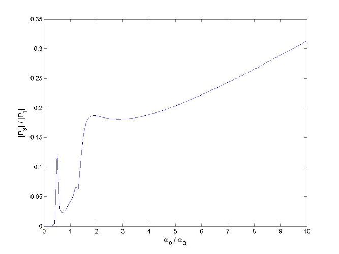
Figure 1: The dependence of $|P_{3}|/|P_{1}|$ on $\omega_{0}/\omega_{3}$ at the distance $x=300\,{\rm cm}$ (the interaction length).

III Summary

The presented results show that the considered nonlinear acoustic process ”feel” very slightly bubble oscillations with low resonance frequencies. Instead bubble oscillations with high resonance frequencies influence significantly nonlinear wave interaction. The generated wave amplitude in this case achieves a measurable value of the tenths of the pump amplitudes at a reasonable distance. The range where $\omega_{0}$ coincides with one of the frequencies of the interacting waves is not favorable for nonlinear acoustic interaction not only because of higher energy losses when bubble oscillations fall in resonance with the interacting acoustic waves, but also because $\omega_{0}$ is not sufficiently high in that interval.

References

• (1) J.M.Hovem, ”The Nonlinearity Parameter of Saturated Marine Sediments,”   J. Acoust. Soc. Am. 66(5), 1463 (1979).
• (2) I.Y.Belyaeva, V.Yu.Zaitsev, and E.M.Timanin, ”Experimental Study of Nonlinear Elastic Properties of Granual Media with Nonideal Packing,”   Acoust.Phys. 40, 789 (1994).
• (3) V.Yu.Zaitsev, A.B.Kolpakov, and V.E.Nazarov, ”Detection of Acoustic Pulses in River sand. Experiment,”   Acoust. Phys. 45,(2), 202 (1999).
• (4) V.Yu.Zaitsev, A.B.Kolpakov, and V.E.Nazarov, ”Detection of Acoustic Pulses in River Sand. Theory,”   Acoust. Phys. 45(2), 305 (1999).
• (5) E.A.Zabolotskaya and S.I.Soluyan, ”A Possible Approach to the Amplification of Sound Waves,”   Sov. Phys.-Acoust. 13, 254 (1967).
• (6) V.G.Welsby and M.H.Safar, ”Acoustic Non-Linearity due to Microbubbles in Water,”   Acustica 22, 177 (1969/70).
• (7) E.A.Zabolotskaya and S.I.Soluyan, ”Nonlinear Wave Propagation in a Fluid with Uniformly Spread Air Bubbles,”   Acoust. Zh. 19, 690 (1973).
• (8) Junru Wu and Zhemin Zhu, ”Measurements of the Effective Nonlinearity Parameter $B/A$ of Water Containing Trapped Cylindrical Bubbles,”   J. Acoust. Soc. Am. 89(6), 2634 (1991).
• (9) D.M.Donskoy and A.M.Sutin, ”Nonlinear Scattering and Propagation of Longitudinal Acoustic Waves in Porous Media,”   Sov. Phys.-Acoust. 30, 358 (1984).
• (10) F.A.Boyle and N.P.Chotiros, ”Nonlinear Acoustic Scattering from a Gassy Poroelastic Seabed,”   J. Acoust. Soc. Am. 103(5), 1328 (1998).
• (11) N.I.Pushkina, ”Nonlinear Three-wave Interaction in Marine Sediments,”   Phys. Wave Phen, 20(3), 1 (2012).
• (12) A.Turgut and T.Yamamoto, ”Measurements of Acoustic Wave Velocities and Attenuation in Marine Sediments,”   J. Acoust. Soc. Am. 87(6), 2376 (1990).
• (13) R.D.Stoll, ”Velocity Dispersion in Water-Saturated Granular Sediment,”  J. Acoust. Soc. Am. , 111(2), 785 (2002).
• (14) N.P.Chotiros and M.J.Isakson, ”A Broadband Model of Sandy Ocean Sediments: Biot-Stoll with Contact Squirt Flow and Shear Drag,”   J. Acoust. Soc. Am. 116(4), 2011 (2004).
• (15) J.L.Buchanan, ”A comparison of Broadband Models for Sand Sediments,”   J. Acoust. Soc. Am. 120(6) 3584 (2006).
• (16) V.G.Bykov and V.N.Nikolaevskii, ”Nonlinear Geoacoustic Waves in Sea Sediments,”  Sov. Phys.-Acoust. 36, 342 (1990).
• (17) N.I.Pushkina, ”Nonlinear Raman-Type Acoustic Scattering in Three-Phase Marine Sediments,”  Acoust. Phys. 47(2), 214 (2001).
• (18) H.Medwin, ”Counting Bubbles Acoustically: a Review,”  Ultrasonics 15(1), 7 (1977).