Plane correlations in small colliding systems

Abstract

I propose event-plane correlations as a test of collectivity in small colliding systems: In d-Au and ³He-Au collisions, I predict a strong anti-correlation between elliptic and triangular flow, generated by the geometry of the light projectile. A significant anti-correlation is also predicted in central p-Pb collisions at the LHC, which is solely generated by fluctuations. Similar, but stronger correlation patterns are predicted in correlations involving dipolar flow.

I Introduction

In high energy nucleus-nucleus collisions, collectivity is best manifested in the measured harmonic flow Heinz and Snellings (2013); Luzum and Petersen (2014). Defined as the Fourier harmonics of a single-particle spectrum,

$$\frac{dN}{d\phi_{p}}=\frac{N}{2\pi}[1+\sum_{n=1}^{\infty}V_{n}e^{-in\phi_{p}}+\text{complex conj.}]\,,$$ (1)

harmonic flow $V_{n}=v_{n}\exp(in\Psi_{n})$ characterises final state anisotropy in the momentum space. Recently, analyses of harmonic flow were extended to small colliding systems, regarding the striking observation of a ridge structure in long-range (in rapidity) two-particle correlations in high multiplicity events Chatrchyan et al. (2013a). At RHIC energy, substantial elliptic flow $v_{2}$ and triangular flow $v_{3}$ were extracted in d-Au and ³He-Au collisions Adare et al. (2013); Huang (2014). At the LHC, in $\sqrt{s_{\mbox{\tiny NN}}}=5.07$ TeV p-Pb collisions, it was also shown that harmonic flow can be as large as that measured in Pb-Pb collisions with $\sqrt{s_{\mbox{\tiny NN}}}=2.76$ TeV Chatrchyan et al. (2013b); Aad et al. (2014a); Abelev et al. (2013), provided that multiplicity yields in these events are comparable Başar and Teaney (2014). The observation of harmonic flow implies a possible collective expansion stage during the collisions of p-Pb, d-Au and ³He-Au, which is further supported by various theoretical simulations. With appropriate descriptions of the initial density profile, reasonable predictions on harmonic flow have been achieved for p-Pb Bozek (2012); Kozlov et al. (2014); Qin and Müller (2014), d-Au Qin and Müller (2014); Nagle et al. (2014) and ³He-Au Nagle et al. (2014); Bozek and Broniowski (2014) colliding systems with viscous hydrodynamics. In a transport approach, it is also found that the prediction of $v_{2}$ and $v_{3}$ requires sufficient interactions in the late stage Bzdak and Ma (2014).

However, the statement of collectivity in small colliding systems is still under debate. In particular, it is challenged by the fact that long-range correlations seen in the experimental data can originate alternatively from pre-equilibrium physics Gyulassy et al. (2014). A way to disentangle competing models, and especially to clarify the issue of collectivity, lies in the measurements of flow fluctuations and mixing between harmonics. The idea relies on the knowledge that medium collectivity associates harmonic flow with event-by-event fluctuations in the initial density profile. The CMS Collaboration has updated its measurements of $v_{2}$ fluctuations in terms of cumulants $v_{2}\{m\}$ from multi-particle correlations Wang (2014); Khachatryan et al. (2015). The observed pattern of $v_{2}\{m\}$ agrees with cumulants of initial ellipticity which is purely driven by fluctuations Yan and Ollitrault (2014); Bzdak et al. (2014), which coincides with the expectation from collective expansion.

This work is motivated in a similar manner, but with emphasis on the mixing of harmonic flow. Especially, event-by-event fluctuations in the initial density profile dominate the mixing between lower harmonics due to a linear eccentricity scaling  Aad et al. (2014b); Teaney and Yan (2014). This allows one to estimate the mixing between $V_{2}$ and $V_{3}$ for p-Pb, d-Au and ³He-Au, in terms of the mixing between initial ellipticity and triangularity. Analyses in this work are focused on central collision events, where the initial state geometries differ dramatically in p-Pb, d-Au and ³He-Au, with the background density profile azimuthally symmetric, dumbbell-shaped and triangle-shaped respectively. In addition, correlations of harmonics involving a dipolar flow $V_{1}$ are studied as well, based on initial mixing involving dipolar asymmetry.

In order to have a consistent comparison with experimental measurements, a series of correlation coefficients are specified in Section II. Collision events are simulated by PHOBOS Monte Carlo Glauber model, with details of the model simulation described in Section III. Correlations of initial anisotropies from simulations are presented in Section III. In Section IV, analytical analysis of the correlations is given based on an independent source approach, where initial state of the small colliding systems are modelled by a number of independent sources. Effects beyond linear eccentricity scaling are discussed with respect to the mixing between $V_{2}$ and $V_{3}$ in p-Pb collisions in Section V.

II Correlation coefficients

In this paper, to quantify correlations between $V_{n}$ and $V_{m}$ (i.e., phase mixing between $\Psi_{n}$ and $\Psi_{m}$ when $n\neq m$), we define the following correlation coefficient which has a similar structure as a Pearson correlation coefficient,

$$\mathcal{P}^{vv}_{nm}=\frac{Re\langle V_{n}^{a}(V_{m}^{*})^{b}\rangle}{\langle|V_{n}|^{2a}\rangle^{1/2}\langle|V_{m}|^{2b}\rangle^{1/2}}\,,$$ (2)

where $a$ and $b$ are integer numbers, satisfying $ma-nb=0$ due to a rotational symmetry. In Eq. (2) and throughout this paper, angular brackets $\langle\ldots\rangle$ are used to notate average over events. By definition one has $0\leq|\mathcal{P}_{nm}^{vv}|\leq 1$, with $1$ stands for an absolute correlation or anti-correlation and $0$ corresponds to pure randomness.

$\mathcal{P}_{nm}^{vv}$ has been studied through the measurements of event-plane correlations in Pb-Pb systems by the ATLAS collaboration Aad et al. (2014b), using the scalar-product method. In particular, the correlation between $V_{2}$ and $V_{3}$,

$$\mathcal{P}^{vv}_{23}=\frac{Re\langle V_{2}^{3}(V_{3}^{*})^{2}\rangle}{\langle|V_{2}|^{6}\rangle^{1/2}\langle|V_{3}|^{4}\rangle^{1/2}}\,,$$ (3)

was found negligibly weak for most of the centralities, except peripheral collisions. Unlike correlations involving higher harmonics, which receive significant contributions from non-linear flow response during medium expansion Teaney and Yan (2014), $\mathcal{P}^{vv}_{23}$ is mostly determined by the mixing between initial anisotropies. Anisotropies of initial state are quantified generally by eccentricities. In each single collision event, if one denotes average over transverse plane according to the initial density profile as $\{\ldots\}$, the first three eccentricities are

$$\mathcal{E}_{1}= \varepsilon_{1}e^{i\Phi_{1}}=-\frac{\{r^{3}e^{i\phi_{r}}\}}{\{r^{3}\}}\,,$$ (4)

$$\mathcal{E}_{2}= \varepsilon_{2}e^{i2\Phi_{2}}=-\frac{\{r^{2}e^{2i\phi_{r}}\}}{\{r^{2}\}}\,,$$ (5)

$$\mathcal{E}_{3}= \varepsilon_{3}e^{i3\Phi_{3}}=-\frac{\{r^{3}e^{3i\phi_{r}}\}}{\{r^{3}\}}\,.$$ (6)

In accordance with Eq. (1), complex notations have been applied in Eqs. (4), (5) and (6), so that both magnitude and phase of eccentricity are defined simultaneously. Approximately a linear eccentricity scaling can be assumed for lower harmonics, based on event-by-event hydrodynamic simulations Niemi et al. (2013),

$$V_{n}=\kappa_{n}\mathcal{E}_{n}\,,\qquad n\leq 3\,.$$ (7)

$\kappa_{n}$ in Eq. (7) is known as the medium response coefficient, which is determined by the property of medium collectivity. It is then obvious that correlations of final state between harmonics are identical to the corresponding correlations of initial anisotropies, e.g.,

$$\mathcal{P}_{23}^{vv}=\mathcal{P}_{23}^{\varepsilon\varepsilon}\,.$$ (8)

Note that the superscript with $\varepsilon$’s on the right hand side of Eq. (8) implies correlations of initial anisotropies.

Mixing between $\mathcal{E}_{2}$ and $\mathcal{E}_{3}$ (or equivalently $V_{2}$ and $V_{3}$) in small colliding systems is of particular interest for two reasons. First, geometrical fluctuations in the initial state are much more pronounced in p-Pb, d-Au and ³He-Au than those in nucleus-nucleus collisions. For instance, the multiplicity in central p-Pb is smaller roughly by a factor of 10 than in central Pb-Pb collisions, one expects initial state fluctuations to be larger by a factor of $\sqrt{10}$. Second, background geometries in d-Au and ³He-Au are generically deformed. For events in the most central collision bins of p-Pb, d-Au and ³He-Au, geometry of the system is dominated by the configuration of proton, deuteron and ³He respectively. Therefore, initial state background geometry of p-Pb is azimuthally symmetric. But for d-Au and ³He-Au, a dumbbell-shaped initial density and an intrinsic triangle-shaped initial density are expected respectively. Accordingly, non-trivial geometries lead to an intrinsic initial ellipticity $\bar{\mathcal{E}}_{2}$ in d-Au and an intrinsic initial triangularity $\bar{\mathcal{E}}_{3}$ in ³He-Au. Both fluctuations and background geometry will be shown essential for the generation of anisotropy correlations, later in Section III and Section IV. Similarly, one also expects fluctuations and geometric shape induce correlations involving a dipolar asymmetry, namely correlations of harmonics involving $V_{1}$. In this paper the following types of correlations are studied as well,

$$\mathcal{P}_{12}^{vv},\quad\mathcal{P}_{13}^{vv}\quad\mbox{and}\quad\mathcal{P}_{123}^{vvv}\,.$$ (9)

Note that $\mathcal{P}_{123}^{vvv}$ is defined as

$$\mathcal{P}_{123}^{vvv}=\frac{Re\langle V_{1}V_{2}V_{3}^{*}\rangle}{\langle|V_{1}V_{2}|^{2}\rangle^{1/2}\langle|V_{3}|^{2}\rangle^{1/2}}\,,$$ (10)

which is normalized differently from the three-plane event-plane correlations introduced by the ATLAS collaboration Aad et al. (2014b) with the scalar-product method.

III Monte Carlo Glauber simulations

In this work, we simulate initial state of heavy-ion collisions using the PHOBOS Monte Carlo Glauber model Alver et al. (2008a); Loizides et al. (2014). Additional modifications are taken into account with respect to small colliding systems. For instance, the wounding profile of two colliding nucleons is taken to be a Gaussian instead of a step function Bozek and Broniowski (2013). Regarding heavy-ion collisions, PHOBOS Glauber model captures the dominant geometric structure and effects of fluctuations of nucleons inside a colliding nucleus. On an event-by-event basis, fluctuations of nucleon positioning inside nucleus are introduced randomly in model simulations, resulting in a discrete distribution of number of participants $N_{part}$ and collisions $N_{coll}$. A Gaussian smearing centered at the location of each participant and collision is applied,

$$\frac{1}{2\pi\sigma^{2}}e^{-|\vec{x}_{\perp}|^{2}/2\sigma^{2}}\,.$$ (11)

The size of smearing is taken to be $\sigma=0.4$ fm and $0.8$ fm in this work for analysis. Initial entropy density is thus obtained by assuming a proper weight associated with each participant and collision,

$$s(x,y,\tau_{o})=C_{s}\left[\frac{1-\alpha}{2}N_{part}(x,y)+\alpha N_{coll}(x,y)\right]\,.$$ (12)

Instead of a constant weighting of $C_{s}$, a negative binomial distribution (NBD) weighting is known necessary to reproduce the measured multiplicity distributions Bozek and Broniowski (2013) in small colliding systems, which introduces extra fluctuations. Especially, probability of generating high multiplicity events is enhanced with a negative binomial weighting. In this work, following Refs.Bozek and Broniowski (2013); Qin and Müller (2014) and taking the same set of parameters for p-Pb at the LHC, and d-Au and ³He-Au at RHIC, ten million events are generated. Events are then classified with respect to number of participants $N_{part}$, which has a correspondence to the centrality classification used in experiments. For simulations with ten million events, the centrality of bin class with reliable statistics can be as small as 0.01%, which corresponds to the right most points in Fig. 1 and Fig. 2.

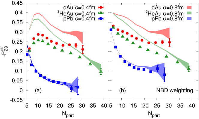
Figure 1: (Color online) Initial state mixing between $\mathcal{E}_{2}$ and $\mathcal{E}_{3}$ as a function of number of participants. Results in panel (a) are from PHOBOS Monte Carlo Glauber model with a constant weighting of $C_{s}$ in Eq. (12). Dashed line is analytical expectation from the independent-source model. Results with an extra NBD weighting is shown in Panel (b). Results from smearing with $\sigma=0.4$ fm are plotted with symbols, while shaded bands correspond to the case with $\sigma=0.8$ fm.

Anti-correlations between $\mathcal{E}_{2}$ and $\mathcal{E}_{3}$ in p-Pb, d-Au and ³He-Au are discovered via model simulations, with results shown in Fig. 1. Note that a minus sign is implied. Panel (a) of Fig. 1 is obtained based on PHOBOS Glauber model, without additional NBD weighting for the entropy production. Albeit less realistic, the case with a constant weighting is closer to the model of independent sources Bhalerao et al. (2011a); Bhalerao and Ollitrault (2006); Blaizot:2014wba, especially for the p-Pb system the correlation $\mathcal{P}_{23}^{\varepsilon\varepsilon}$ is found quantitatively consistent with predictions from independent sources (see discussions around Eq. (16) in Section IV). Simulations with NBD weighting which correspond to experiments carried out at RHIC and the LHC are presented in Fig. 1 (b). Errors of these results are estimated based on variance. Effect of smearing is investigated with $\sigma=0.4$ fm (symbols with error bars) and $\sigma=0.8$ fm (shaded bands). Larger smearing size leads to stronger correlations between $\mathcal{E}_{2}$ and $\mathcal{E}_{3}$, which is more significant for d-Au and ³He-Au systems.

In all three colliding systems, the correlation between $\mathcal{E}_{2}$ and $\mathcal{E}_{3}$ decreases towards central collisions. This decrease is associated with the decrease of fluctuations in the initial state. When extra fluctuations are introduced from a NBD weighting of entropy production, seen as changes from Fig. 1 (a) to Fig. 1 (b), correlations are enhanced as well. Especially for p-Pb, the correlation of the most central events reaches 10%, as shown in Fig. 1 (b). In addition, from Fig. 1 there is an apparent hierarchy relation of correlations among the three systems,

$$|\mathcal{P}_{23}^{\varepsilon\varepsilon}(\mbox{p-Pb})|<|\mathcal{P}_{23}^{\varepsilon\varepsilon}(^{3}\mbox{He-Au})|<|\mathcal{P}_{23}^{\varepsilon\varepsilon}(\mbox{d-Au})|$$ (13)

which reflects the differences in the background geometry of each system. One may naïvely understand this relation by noticing that $\mathcal{E}_{2}$ has one power higher than $\mathcal{E}_{3}$ in the original definition of $\mathcal{P}_{23}^{\varepsilon\varepsilon}$, which makes a backgound ellipticitiy more important than a background triangularity. More detailed discussion of this hierarchy relation are given in Section IV.

Figure 2: (Color online) Initial state mixing involving $\mathcal{E}_{1}$ as a function of number of participants, represented by (a) $\mathcal{P}^{\varepsilon\varepsilon}_{12}$, (b) -$\mathcal{P}^{\varepsilon\varepsilon}_{13}$, and (c) -$\mathcal{P}^{\varepsilon\varepsilon}_{123}$. All the results are obtained with an extra NBD weighting for the entropy production. Results with $\sigma=0.4$ fm are plotted with symbols, while shaded bands correspond to $\sigma=0.8$ fm.

Fig. 2 presents initial correlations involving $\mathcal{E}_{1}$, as predictions for the flow correlations involving $V_{1}$. Again, to have all results on the same scale a minus sign is applied when necessary. Irrespective of the detailed background geometry, in all the three systems a negative $\mathcal{P}_{12}^{\varepsilon\varepsilon}$ and a negative $\mathcal{P}_{123}^{\varepsilon\varepsilon\varepsilon}$ are obtained which indicate anti-correlations between $\mathcal{E}_{1}$ and $\mathcal{E}_{2}$, and among $\mathcal{E}_{1}$, $\mathcal{E}_{2}$ and $\mathcal{E}_{3}$ respectively, while $\mathcal{E}_{1}$ and $\mathcal{E}_{3}$ are found strongly correlated. Although these correlations are stronger than $\mathcal{P}_{23}^{\varepsilon\varepsilon}$, they exhibit very similar dependence on the background geometry of the system and fluctuations, i.e., similar hierarchy relations regarding the three systems. More detailed discussions are postponed to Section IV. It is also worth mentioning that for the most central events in d-Au systems, correlations from simulations are compatible with those expected in peripheral nucleus-nucleus collisions Bhalerao et al. (2011b); Teaney and Yan (2011); Jia and Mohapatra (2013), where the effects of fluctuations are comparable.

Measuring event-plane correlations in small collision systems is a challenging analysis. In Appendix A, we evaluate the order of magnitude of the statistical error. We find that in order to detect $\mathcal{P}_{23}^{vv}$ with a few percent accuracy in p-Pb central collisions at the LHC, one typically needs a million events per centrality bin.

IV Understanding of initial state correlations

Figure 3: (Color online) Alignment of anisotropies due to fluctuations on top of smooth background (solid blue shape) with a net ellipticity $\mathcal{E}_{2}$ (a) and a net triangularity $\mathcal{E}_{3}$ (b). Green dashed shapes correspond to anisotropies generated by one addition hot spot in the tip area of the background. Dipolar asymmetry is illustrated as green arrows.

The origin of anisotropy correlations in the initial state of heavy-ion collisions, with respect to the effects of fluctuations and a background geometry, can be understood qualitatively as follows. In heavy-ion collisions, a bumpy initial state density profile can be equivalently realized by randomly throwing additional spots on top of a smooth background. For a smooth background with a net ellipticity or triangularity, the area of tip is always larger than that of side, which is purely a consequence of geometric effect. Therefore, one expects the additional spots to appear more probably in the area of tip rather than side. Fig. 3 describes anisotropies induced by one additional hot spot in the tip area of an elliptic background (a), and a triangular background (b). In both cases, one can check that the induced anisotropies are aligned with the background shape in a specified way: $\Phi_{1}=\pi$, $\Phi_{2}=\pi/2$, and $\Phi_{3}=\pi/3$, which generates perfect anti-correlations between $\mathcal{E}_{2}$ and $\mathcal{E}_{3}$, $\mathcal{E}_{1}$ and $\mathcal{E}_{2}$, and among $\mathcal{E}_{1}$, $\mathcal{E}_{2}$ and $\mathcal{E}_{3}$, and perfect correlation between $\mathcal{E}_{1}$ and $\mathcal{E}_{3}$. For a more sophisticated density profile which fluctuates from event to event, correlations are weaken due to contributions from configurations with excessive density around sides of the background shape, but the sign of correlation should not be changed.

To a quantitative level, the effects of fluctuations and background geometry on correlations can be studied in the independent-source model Bhalerao et al. (2011a), in which an initial state density profile is modelled by N point-like independent sources on top of a specified background. Consequently, fluctuations of any quantity $f$ is characterized as

$$\delta_{f}=\{f\}-\langle f\rangle\,,$$ (14)

where $\{\ldots\}$ and $\langle\ldots\rangle$ are used in the similar way as in Eqs. (4) and (2), indicating average in the transverse plane for one single event and average over events respectively. Independency of sources allows one to write event averaged quantities in powers of $1/N$, i.e., fluctuations. For instance, the two-point function which quantifies event average of quadratic order of fluctuations, is of the order of $1/N$,

$$\langle\delta_{f}\delta_{g}\rangle=\frac{\langle fg\rangle-\langle f\rangle\langle g\rangle}{N}\,.$$ (15)

Event average of higher order of fluctuations leads to higher order dependence on $1/N$. More details of the model can be found in Bhalerao et al. (2011a) and in Appendix B. For p-Pb collisions, background is azimuthally symmetric and thus $\bar{\mathcal{E}}_{2}=\bar{\mathcal{E}}_{3}=0$. One accordingly finds that the dominant contribution is purely driven by fluctuations, and of the order of $1/N^{3/2}$,

$$\mathcal{P}_{23}^{\varepsilon\varepsilon}(\mbox{p-Pb})=-\frac{1}{N^{3/2}}\frac{\langle r^{12}\rangle+6\langle r^{6}\rangle^{2}-18\langle r^{4}\rangle\langle r^{8}\rangle}{\sqrt{12}\langle r^{4}\rangle^{3/2}\langle r^{6}\rangle}+O(1/N^{5/2})\,.$$ (16)

For a Gaussian smearing, the geometric factor in Eq. (16) is known explicitly ($\approx 1.22$) and thus an analytical description can be obtained. As shown as the blue dashed line in Fig. 1 (a), the prediction from independent sources naturally captures the correlation pattern if one assumes that the number of independent sources scales like $N_{part}\sim 0.55N$. Note also that in Eq. (16) the correlation is insensitive to a Gaussian smearing, which is indeed confirmed in Fig. 1 that smearing $\sigma$ has little influence on the simulated correlation $\mathcal{P}_{23}^{\varepsilon\varepsilon}(\mbox{p-Pb})$.

In principle, the generic correlations induced by the nuclear configurations of deuteron and ³He prevent applying the independent-source model to the collisions of d-Au and ³He-Au. Nevertheless, the effect of a non-trivial background geometry is worth analyzing, at least qualitatively. For ³He-Au collisions, the conditions $\bar{\mathcal{E}}_{2}=0$ and $\bar{\mathcal{E}}_{3}\neq 0$ allow terms of lower order in $1/N$ contribute. While for d-Au systems, a non-zero background ellipticity picks up even lower order terms in the expansion with respect to $1/N$. It can also be understood directly from the definition of $\mathcal{P}_{23}^{\varepsilon\varepsilon}\sim\langle\mathcal{E}_{2}^{3}(\mathcal{E}_{3}^{*})^{2}\rangle$, that $\mathcal{E}_{2}$ has one power higher than $\mathcal{E}_{3}$. In total, counting the extra suppression due to fluctuations, one finds

$$|\mathcal{P}_{23}^{\varepsilon\varepsilon}(^{3}\mbox{He-Au})|\sim O\left(\frac{1}{N^{1/2}}\right),\qquad|\mathcal{P}_{23}^{\varepsilon\varepsilon}(\mbox{d-Au})|\sim O(1)\,,$$ (17)

which is consistent with Eq. (13). It is also interesting to notice that the hierarchy relation in Eq. (13) disappears when $N_{part}$ is sufficiently small, as depicted in Fig. 1, where only one of the constituent nucleons in deuteron and ³He participates the collision.

For correlations involving a dipolar asymmetry, an ideal assumption would be taking $\mathcal{E}_{1}$ as a result of fluctuations in all the three small systems, then the similar argument leads to

$$|\mathcal{P}_{123}^{\varepsilon\varepsilon\varepsilon}(\mbox{d-Au})|\sim|\mathcal{P}_{123}^{\varepsilon\varepsilon\varepsilon}(^{3}\mbox{He-Au})|\sim O(1)\,,\qquad|\mathcal{P}_{123}^{\varepsilon\varepsilon\varepsilon}(\mbox{p-Pb})|\sim O\left(\frac{1}{\sqrt{N}}\right)\,,$$ (18)

due to the fact that $\mathcal{E}_{2}$ and $\mathcal{E}_{3}$ are of the same power in the definition of $\mathcal{P}_{123}^{\varepsilon\varepsilon\varepsilon}$. And indeed Eq. (18) agrees with the results depicted in Fig. 2 (c). However, when the role of $\mathcal{E}_{1}$ becomes more important, as in $\mathcal{P}_{12}^{\varepsilon\varepsilon}$ and $\mathcal{P}_{13}^{\varepsilon\varepsilon}$ which contain $\mathcal{E}_{1}^{2}$ and $\mathcal{E}_{1}^{3}$ respectively, one has to take into account the effect of an intrinsic $\bar{\mathcal{E}}_{1}$ in both d-Au and ³He-Au . Because a larger intrinsic $\bar{\mathcal{E}}_{1}$ is expected with repect to a dumbbell-shape than a triangular shape, the correlations $\mathcal{P}_{12}^{\varepsilon\varepsilon}$ and $\mathcal{P}_{13}^{\varepsilon\varepsilon}$ are stronger in d-Au than in ³He-Au.

V $\mathcal{P}_{23}^{vv}$ in proton-lead beyond linear eccentricity scaling

One must go beyond the approximate linear eccentricity scaling to have a more realistic estimate for the correlations of harmonics in experiments. For the central p-Pb collisions, non-linear flow response can still be ignored since background geometry is azimuthally symmetric, which case is similar to the ultra-central Pb-Pb. The most significant corrections come from fluctuations in hydro response. While detailed knowledge of event-by-event fluctuations of flow response requires a systematic analysis based on, e.g., event-by-event hydrodynamic simulations, it can be quantified by introducing an extra noise term in Eq. (7) Yan et al. (2015); Gardim et al. (2012)

$$V_{n}=\kappa_{n}\mathcal{E}_{n}+X_{n}\,,$$ (19)

where the noise $X_{n}$ is complex. I further model $X_{n}$ as a Gaussian noise, which is uncorrelated with the initial eccentricity. This noise breaks linear eccentricity scaling Niemi et al. (2013). The magnitude of the effect can be quantified by the Pearson correlation between the flow and the initial anisotropy,

$$\frac{\langle V_{n}\mathcal{E}_{n}^{*}\rangle}{\langle|V_{n}|^{2}\rangle^{1/2}\langle|\mathcal{E}_{n}|^{2}\rangle^{1/2}}=1-\lambda_{n}+O(\lambda_{n}^{2})\,,$$ (20)

where

$$\lambda_{n}=\frac{1}{2}\frac{\langle|X_{n}|^{2}\rangle}{\kappa_{n}^{2}\langle|\mathcal{E}_{n}|^{2}\rangle}\,,$$ (21)

is a small and positive quantity, characterizing the relative magnitude between fluctuations and average flow response. For the correlation between $V_{2}$ and $V_{3}$, substituting Eq. (19) into Eq. (3) results in

$$\mathcal{P}_{23}^{vv}=\mathcal{P}_{23}^{\varepsilon\varepsilon}\left[1-\frac{9\langle|\mathcal{E}_{2}^{4}|\rangle\langle|\mathcal{E}_{2}|^{2}\rangle}{\langle|\mathcal{E}_{2}|^{6}\rangle}\lambda_{2}-\frac{4\langle|\mathcal{E}_{3}|^{2}\rangle^{2}}{\langle|\mathcal{E}_{3}|^{4}\rangle}\lambda_{3}+O(\lambda^{2})\right]\,.$$ (22)

The factors before $\lambda_{2}$ and $\lambda_{3}$ in Eq. (22) are determined by fluctuations of $\mathcal{E}_{2}$ and $\mathcal{E}_{3}$ respectively. In p-Pb collisions, it was proposed that fluctuations of initial state eccentricities follow the so-called power distribution Yan and Ollitrault (2014), from which the ratios between moments of initial state eccentricity are known explicitly. In central collision events, approximately one has $9\langle|\mathcal{E}_{2}^{4}|\rangle\langle|\mathcal{E}_{2}|^{2}\rangle/\langle|\mathcal{E}_{2}|^{6}\rangle\approx 3$ and $4\langle|\mathcal{E}_{3}|^{2}\rangle^{2}/\langle|\mathcal{E}_{3}|^{4}\rangle\approx 2$.

An estimate of $\lambda_{2}$ and $\lambda_{3}$ in p-Pb collisions at the LHC can be made in terms of the breaking of two-particle correlations. Fluctuations in hydro response result in a breaking in the two-particle correlation function, which is characterised by the ratio Gardim et al. (2013),

$$r_{n}(p_{T}^{a},p_{T}^{b})=\frac{V_{n\Delta}(p_{T}^{a},p_{T}^{b})}{\sqrt{V_{n\Delta}(p_{T}^{a},p_{T}^{a})V_{n\Delta}(p_{T}^{b},p_{T}^{b})}}\,.$$ (23)

Taking into account noise in hydro response in Eq. (19), one obtains

$$r_{n}(p_{T}^{a},p_{T}^{b})=1-\lambda_{n}(p_{T}^{a})-\lambda_{n}(p_{T}^{b})+O(\lambda^{2}).$$ (24)

For the central collision events in the available $p_{T}$ range, $r_{2}(p_{T}^{a},p_{T}^{b})$ from event-by-event hydrodynamic simulations can reach as low as 97% Kozlov et al. (2014), depending on smearing size and shear viscosity over entropy ratio $\eta/s$ used in simulations. Consequently, one would expect that the integrated value of $\lambda_{2}$ to be smaller than 3%. Similarly, the upper bound of $\lambda_{3}$ can be taken as 5%.

In total, for the central events of p-Pb, correlation between $V_{2}$ and $V_{3}$ is expected with a value greater than 8% if late stage collective expansion indeed dominates the evolution.

VI Conclusions

In summary, I have studied correlations between harmonics in the small colliding systems: p-Pb, d-Au and ³He-Au. Emphasis is laid on the mixing between $V_{2}$ and $V_{3}$, in terms of mixing between ellipticity $\mathcal{E}_{2}$ and triangularity $\mathcal{E}_{3}$, by assuming linear eccentricity scaling. Significant anti-correlations are found between $\mathcal{E}_{2}$ and $\mathcal{E}_{3}$ in p-Pb systems from Monte Carlo Glauber simulations, with $|\mathcal{P}_{23}^{\varepsilon\varepsilon}|$ of the order of 10% in the central collision events. When the background geometry exhibits an intrinsic ellipticity, such as central d-Au collisions, or an intrinsic triangularity, such as central ³He-Au collisions, the correlation is even enhanced. Monte Carlo Glauber simulations present stronger anti-correlation of $\mathcal{P}_{23}^{\varepsilon\varepsilon}$ in d-Au than that in ³He-Au. Similar, but stronger correlation patterns are found when the dipolar asymmetry $\mathcal{E}_{1}$ is involved. The physical origin of initial state correlations is analytically studied in the independent-source model, from which fluctuations and intrinsic shape are recognized as the dominant effects.

Mixing between harmonic flow is basically considered equal to the corresponding mixing of initial anisotropies, due to an approximate linear eccentricity scaling. Effects beyond linear eccentricity scaling are discussed by including noises in the linear flow response, from which a more realistic estimate of $\mathcal{P}_{23}^{vv}$ is made for the central p-Pb collisions. Regarding measurements carried out by the CMS collaboration, statistics in experiment is discussed in Appendix A. Mixing between $V_{2}$ and $V_{3}$ is thus proposed as an accessible probe to detect the medium collectivity in experiments, if evolution in p-Pb collisions is dominated by the medium collective expansion. In d-Au and ³He-Au, especially in the most central events, medium collectivity is supposed to lead to sizable $\mathcal{P}_{23}^{vv}$ as well, although its patterns may be more involved due to other effects like non-linearities in the flow generation. However, geometries of p-Pb, d-Au and ³He-Au systems are expected to be revealed by comparing $\mathcal{P}_{23}^{vv}$ among these colliding systems. In a similar manner, correlations involving $V_{1}$ are proposed as probes as well, which are generated from initial correlations involving $\mathcal{E}_{1}$.

Appendix A Statistical errors of $\mathcal{P}_{23}^{vv}$ measurements in p-Pb

In this appendix, I briefly estimate the statistical error on $\mathcal{P}_{23}^{vv}$ in the central p-Pb collisions at the LHC. The order of magnitude of the number of events that is needed for the observation of $\mathcal{P}_{23}^{vv}$ in experiments can be inferred consequently. The measurement of $\mathcal{P}_{23}^{vv}$ involves a five-particle correlation,

$$\langle V_{2}^{3}(V_{3}^{*})^{2}\rangle$$ (25)

whose statistical error is determined by the total number of independent 5-plets which can be constructed. For a total number of events $N_{eve}$ and multiplicity $M$ in each single event, statistical fluctuations with respect to $\langle V_{2}^{3}(V_{3}^{*})^{2}\rangle$ are therefore of the order $1/(N_{eve}M^{5})^{1/2}$. Statistical errors on $\mathcal{P}_{23}^{vv}$ from measurements can be accordingly estimated as

$$\delta\mathcal{P}_{23}^{vv}\sim\frac{1}{\sqrt{N_{eve}}}\left(\frac{1}{v_{2}\sqrt{M}}\right)^{3}\left(\frac{1}{v_{3}\sqrt{M}}\right)^{2}\,.$$ (26)

The rule of thumb of writing Eq. (26) is that each $V_{n}$ contributes a factor $1/(|V_{n}|\sqrt{M})$. Similar analysis can be generalized to the measurements of other types of correlations between harmonics.

Referring to the measurements of p-Pb carried out by the CMS collaboration Chatrchyan et al. (2013b); Khachatryan et al. (2015), the resolution of $v_{2}$ and $v_{3}$ measurements for central collisions are approximately $(1/v_{2}\sqrt{M})\sim 1.25$ and $(1/v_{3}\sqrt{M})\sim 5$ respectively. In total, to observe $\mathcal{P}_{23}^{vv}$ with value at least 8%, a total number of one million events are roughly needed for each centrality bin. The LHC has already recorded an integrated luminosity of 35nb^-1(cf. Ref. Khachatryan et al. (2015)) in the p-Pb runs collected in 2012 and 2013, corresponding to a total events of the order of $10^{10}$. Therefore there are over one million events in the 0.01% most central bin, and the anti-correlation between $V_{2}$ and $V_{3}$ can be detected as a feasible probe for the test of medium collectivity.

Appendix B $\mathcal{P}_{23}^{\varepsilon\varepsilon}$ from independent sources

We take complex notations for simplicity in the following derivations, so that the transverse coordinate is expressed as $z=r\exp{(i\phi_{r})}$. In the independent-source model, azimuthal eccentricities of a fluctuating initial state can be analytically written. Taking into account of the re-centering corrections,

$$\mathcal{E}_{2}= \varepsilon_{2}e^{i2\Phi_{2}}=-\frac{\{(z-\delta_{z})^{2}\}}{\{r^{2}\}}\,,$$

$$\mathcal{E}_{3}= \varepsilon_{3}e^{i3\Phi_{3}}=-\frac{\{(z-\delta_{z})^{3}\}}{\{r^{3}\}}\,.$$ (27)

Eq. (B) can be expanded with respect to fluctuations order by order, which in turn gives rise to an expansion in terms of $1/N$. Therefore we have,

$$\mathcal{E}_{2}= -\frac{[\langle z^{2}\rangle+\delta_{z^{2}}+\delta_{z}^{2}]}{\langle r^{2}\rangle}+O(\delta^{3})\,,$$

$$\mathcal{E}_{3}= -\frac{[\langle z^{3}\rangle-3\langle z^{2}\rangle\delta_{z}+\delta_{z^{3}}-3\delta_{z}\delta_{z^{2}}]}{\langle r^{3}\rangle}+O(\delta^{3})\,.$$ (28)

Note that $\langle z^{2}\rangle=-\langle r^{2}\rangle{\bar{\mathcal{E}}}_{2}$ or $\langle z^{3}\rangle=-\langle r^{3}\rangle{\bar{\mathcal{E}}}_{3}$ in Eq. (B) vanishes when there is no corresponding intrinsic eccentricity from the background geometry. For simplicity, contributions from fluctuations of denominators in Eq. (B) are neglected, which does not affect the counting of power of fluctuations and is allowed quantitatively for p-Pb.

In the independent source model, in addition to the two-point function in Eq. (15) which is proportional to $1/N$, multi-point function can be evaluated using Wick’s theorem, and found to be suppressed by higher powers of $1/N$ Alver et al. (2008b). Implicitly, one has

$$\langle\delta^{3}\rangle\sim\langle\delta^{4}\rangle\sim O\left(\frac{1}{N^{2}}\right),\quad\langle\delta^{5}\rangle\sim\langle\delta^{6}\rangle\sim O\left(\frac{1}{N^{3}}\right),\ldots\,.$$ (29)

Pearson coefficients of initial state Eq. (2) can therefore be written order by order in powers of $1/N$. For the p-Pb systems, because all terms proportional to $\langle z^{2}\rangle$ or $\langle z^{3}\rangle$ vanish, one has

$$\mathcal{P}_{23}^{\varepsilon\varepsilon}=-\frac{\langle\delta_{z^{2}}^{3}\delta_{{\bar{z}}^{3}}^{2}\rangle+3\langle\delta_{z^{2}}^{2}\delta_{z}^{2}\delta_{{\bar{z}}^{3}}^{2}\rangle-6\langle\delta_{z^{2}}^{3}\delta_{\bar{z}}\delta_{{\bar{z}}^{2}}\delta_{{\bar{z}}^{3}}\rangle+O(\langle\delta^{7}\rangle)}{\left[\langle\delta_{z^{2}}^{3}\delta_{{\bar{z}}^{2}}^{3}\rangle+O(\langle\delta^{7}\rangle)\right]^{1/2}\left[\langle\delta_{z^{3}}^{2}\delta_{{\bar{z}}^{3}}^{2}\rangle+O(\langle\delta^{5}\rangle)\right]^{1/2}}\sim\frac{1}{N^{3/2}}\,.$$ (30)

The minus sign in Eq. (30) comes from convention used in the definition of anisotropies and $\mathcal{P}_{23}^{vv}$, which agrees with the analysis given in Section IV. Again, in evaluating multi-point functions, azimuthal symmetry in p-Pb demands that only terms of the type $\langle r^{2n}\rangle=\langle z^{n}{\bar{z}}^{n}\rangle$ left, which leads to the result in Eq. (16). For ³He-Au, terms containing $\langle z^{3}\rangle$ contribute. Besides, terms of the type $\langle z^{a}{\bar{z}}^{b}\rangle\neq 0$ also contribute if $|a-b|/3=0$, 1, etc., which leads to

$$\mathcal{P}_{23}^{\varepsilon\varepsilon}= -\frac{\langle{\bar{z}}^{3}\rangle^{2}\langle\delta_{z^{2}}^{3}\rangle+3\langle{\bar{z}}^{3}\rangle^{2}\langle\delta_{z^{2}}^{2}\delta_{z}^{2}\rangle+2\langle{\bar{z}}^{3}\rangle\langle\delta_{{\bar{z}}^{3}}\delta_{z^{2}}^{3}\rangle+O(\langle\delta^{5}\rangle)}{\left[\langle z^{3}\rangle^{2}\langle{\bar{z}}^{3}\rangle^{2}+O(\langle\delta^{2}\rangle)\right]^{1/2}\left[\langle\delta_{z^{3}}^{2}\delta_{{\bar{z}}^{3}}^{2}\rangle+O(\langle\delta^{5}\rangle)\right]^{1/2}}$$

$$= -\frac{\langle{\bar{z}}^{3}\rangle^{2}\langle z^{6}\rangle+6\langle z^{3}\rangle^{2}\langle{\bar{z}}^{3}\rangle^{2}}{\sqrt{6N}\langle z^{3}\rangle\langle{\bar{z}}^{3}\rangle\langle r^{4}\rangle^{3/2}}+O\left(\frac{1}{N^{3/2}}\right)\,.$$ (31)

For d-Au collisions, $\langle z^{2}\rangle\neq 0$ and accordingly all terms of the type $\langle z^{a}{\bar{z}}^{b}\rangle\neq 0$ if $|a-b|$ is a even integer. One finds that the lowest order term is independent of $1/N$,

$$\mathcal{P}_{23}^{\varepsilon\varepsilon}=-\frac{\langle z^{2}\rangle^{3}\left(9\langle{\bar{z}}^{2}\rangle^{3}+\langle{\bar{z}}^{6}\rangle-6\langle{\bar{z}^{2}}\rangle\langle{\bar{z}^{4}}\rangle\right)}{\left[81\langle z^{2}\rangle^{2}\langle{\bar{z}}^{2}\rangle^{2}\left(2\langle z{\bar{z}}\rangle^{2}+\langle z^{2}\rangle\langle{\bar{z}}^{2}\rangle\right)+2\langle z^{3}{\bar{z}}^{3}\rangle^{2}+\ldots\right]^{1/2}}+O\left(\frac{1}{\sqrt{N}}\right)$$ (32)

References

- Heinz and Snellings (2013) Ulrich Heinz and Raimond Snellings, “Collective flow and viscosity in relativistic heavy-ion collisions,” Ann.Rev.Nucl.Part.Sci. 63, 123–151 (2013), arXiv:1301.2826 [nucl-th] .
- Luzum and Petersen (2014) Matthew Luzum and Hannah Petersen, “Initial State Fluctuations and Final State Correlations in Relativistic Heavy-Ion Collisions,” J.Phys. G41, 063102 (2014), arXiv:1312.5503 [nucl-th] .
- Chatrchyan et al. (2013a) Serguei Chatrchyan et al. (CMS Collaboration), “Observation of long-range near-side angular correlations in proton-lead collisions at the LHC,” Phys.Lett. B718, 795–814 (2013a), arXiv:1210.5482 [nucl-ex] .
- Adare et al. (2013) A. Adare et al. (PHENIX Collaboration), “Quadrupole Anisotropy in Dihadron Azimuthal Correlations in Central Au Collisions at =200 GeV,” Phys.Rev.Lett. 111, 212301 (2013), arXiv:1303.1794 [nucl-ex] .
- Huang (2014) Shengli Huang, “Highlight of phenix results,” (2014), talk at Initial Stages 2014.
- Chatrchyan et al. (2013b) Serguei Chatrchyan et al. (CMS Collaboration), “Multiplicity and transverse momentum dependence of two- and four-particle correlations in pPb and PbPb collisions,” Phys.Lett. B724, 213–240 (2013b), arXiv:1305.0609 [nucl-ex] .
- Aad et al. (2014a) Georges Aad et al. (ATLAS Collaboration), “Measurement of long-range pseudorapidity correlations and azimuthal harmonics in TeV proton-lead collisions with the ATLAS detector,” Phys.Rev. C90, 044906 (2014a), arXiv:1409.1792 [hep-ex] .
- Abelev et al. (2013) Betty Bezverkhny Abelev et al. (ALICE Collaboration), “Long-range angular correlations of , K and p in p-Pb collisions at = 5.02 TeV,” Phys.Lett. B726, 164–177 (2013), arXiv:1307.3237 [nucl-ex] .
- Başar and Teaney (2014) Gökçe Başar and Derek Teaney, “Scaling relation between pA and AA collisions,” Phys.Rev. C90, 054903 (2014), arXiv:1312.6770 [nucl-th] .
- Bozek (2012) Piotr Bozek, “Collective flow in p-Pb and d-Pd collisions at TeV energies,” Phys.Rev. C85, 014911 (2012), arXiv:1112.0915 [hep-ph] .
- Kozlov et al. (2014) Igor Kozlov, Matthew Luzum, Gabriel Denicol, Sangyong Jeon, and Charles Gale, “Transverse momentum structure of pair correlations as a signature of collective behavior in small collision systems,” (2014), arXiv:1405.3976 [nucl-th] .
- Qin and Müller (2014) Guang-You Qin and Berndt Müller, “Elliptic and triangular flow anisotropy in deuteron-gold collisions at GeV at RHIC and in proton-lead collisions at TeV at the LHC,” Phys.Rev. C89, 044902 (2014), arXiv:1306.3439 [nucl-th] .
- Nagle et al. (2014) J. L. Nagle, A. Adare, S. Beckman, T. Koblesky, J. Orjuela Koop, et al., “Exploiting Intrinsic Triangular Geometry in Relativistic He3+Au Collisions to Disentangle Medium Properties,” Phys.Rev.Lett. 113, 112301 (2014), arXiv:1312.4565 [nucl-th] .
- Bozek and Broniowski (2014) Piotr Bozek and Wojciech Broniowski, “Collective flow in ultrarelativistic 3He-Au collisions,” Phys.Lett. B739, 308–312 (2014), arXiv:1409.2160 [nucl-th] .
- Bzdak and Ma (2014) Adam Bzdak and Guo-Liang Ma, “Elliptic and triangular flow in +Pb and peripheral Pb+Pb collisions from parton scatterings,” Phys.Rev.Lett. 113, 252301 (2014), arXiv:1406.2804 [hep-ph] .
- Gyulassy et al. (2014) M. Gyulassy, P. Levai, I. Vitev, and T.S. Biro, “Non-Abelian Bremsstrahlung and Azimuthal Asymmetries in High Energy Reactions,” Phys.Rev. D90, 054025 (2014), arXiv:1405.7825 [hep-ph] .
- Wang (2014) Quan Wang (CMS Collaboration), “Azimuthal anisotropy of charged particles from multiparticle correlations in pPb and PbPb collisions with CMS,” Nucl.Phys. A931, 997–1001 (2014).
- Khachatryan et al. (2015) Vardan Khachatryan, Albert M Sirunyan, Armen Tumasyan, Wolfgang Adam, Thomas Bergauer, et al., “Evidence for collective multi-particle correlations in pPb collisions,” (2015), arXiv:1502.05382 [nucl-ex] .
- Yan and Ollitrault (2014) Li Yan and Jean-Yves Ollitrault, “Universal fluctuation-driven eccentricities in proton-proton, proton-nucleus and nucleus-nucleus collisions,” Phys.Rev.Lett. 112, 082301 (2014), arXiv:1312.6555 [nucl-th] .
- Bzdak et al. (2014) Adam Bzdak, Piotr Bozek, and Larry McLerran, “Fluctuation induced equality of multi-particle eccentricities for four or more particles,” Nucl.Phys. A927, 15–23 (2014), arXiv:1311.7325 [hep-ph] .
- Aad et al. (2014b) Georges Aad et al. (ATLAS Collaboration), “Measurement of event-plane correlations in TeV lead-lead collisions with the ATLAS detector,” Phys.Rev. C90, 024905 (2014b), arXiv:1403.0489 [hep-ex] .
- Teaney and Yan (2014) D. Teaney and L. Yan, “Event-plane correlations and hydrodynamic simulations of heavy ion collisions,” Phys.Rev. C90, 024902 (2014), arXiv:1312.3689 [nucl-th] .
- Niemi et al. (2013) H. Niemi, G.S. Denicol, H. Holopainen, and P. Huovinen, “Event-by-event distributions of azimuthal asymmetries in ultrarelativistic heavy-ion collisions,” Phys.Rev. C87, 054901 (2013), arXiv:1212.1008 [nucl-th] .
- Alver et al. (2008a) B. Alver, M. Baker, C. Loizides, and P. Steinberg, “The PHOBOS Glauber Monte Carlo,” (2008a), arXiv:0805.4411 [nucl-ex] .
- Loizides et al. (2014) C. Loizides, J. Nagle, and P. Steinberg, “Improved version of the PHOBOS Glauber Monte Carlo,” (2014), arXiv:1408.2549 [nucl-ex] .
- Bozek and Broniowski (2013) Piotr Bozek and Wojciech Broniowski, “Collective dynamics in high-energy proton-nucleus collisions,” Phys.Rev. C88, 014903 (2013), arXiv:1304.3044 [nucl-th] .
- Bhalerao et al. (2011a) Rajeev S. Bhalerao, Matthew Luzum, and Jean-Yves Ollitrault, “Understanding anisotropy generated by fluctuations in heavy-ion collisions,” Phys.Rev. C84, 054901 (2011a), arXiv:1107.5485 [nucl-th] .
- Bhalerao and Ollitrault (2006) Rajeev S. Bhalerao and Jean-Yves Ollitrault, “Eccentricity fluctuations and elliptic flow at RHIC,” Phys.Lett. B641, 260–264 (2006), arXiv:nucl-th/0607009 [nucl-th] .
- Bhalerao et al. (2011b) Rajeev S. Bhalerao, Matthew Luzum, and Jean-Yves Ollitrault, “Determining initial-state fluctuations from flow measurements in heavy-ion collisions,” Phys.Rev. C84, 034910 (2011b), arXiv:1104.4740 [nucl-th] .
- Teaney and Yan (2011) Derek Teaney and Li Yan, “Triangularity and Dipole Asymmetry in Heavy Ion Collisions,” Phys.Rev. C83, 064904 (2011), arXiv:1010.1876 [nucl-th] .
- Jia and Mohapatra (2013) Jiangyong Jia and Soumya Mohapatra, “A Method for studying initial geometry fluctuations via event plane correlations in heavy ion collisions,” Eur.Phys.J. C73, 2510 (2013), arXiv:1203.5095 [nucl-th] .
- Yan et al. (2015) Li Yan, Jean-Yves Ollitrault, and Arthur M. Poskanzer, “Azimuthal Anisotropy Distributions in High-Energy Collisions,” Phys.Lett. B742, 290 (2015), arXiv:1408.0921 [nucl-th] .
- Gardim et al. (2012) Fernando G. Gardim, Frederique Grassi, Matthew Luzum, and Jean-Yves Ollitrault, “Mapping the hydrodynamic response to the initial geometry in heavy-ion collisions,” Phys.Rev. C85, 024908 (2012), arXiv:1111.6538 [nucl-th] .
- Gardim et al. (2013) Fernando G. Gardim, Frederique Grassi, Matthew Luzum, and Jean-Yves Ollitrault, “Breaking of factorization of two-particle correlations in hydrodynamics,” Phys.Rev. C87, 031901 (2013), arXiv:1211.0989 [nucl-th] .
- Alver et al. (2008b) B. Alver, B.B. Back, M.D. Baker, M. Ballintijn, D.S. Barton, et al., “Importance of correlations and fluctuations on the initial source eccentricity in high-energy nucleus-nucleus collisions,” Phys.Rev. C77, 014906 (2008b), arXiv:0711.3724 [nucl-ex] .