Evolution of magnetic helicity and energy spectra of solar active regions

Abstract

We adopt an isotropic representation of the Fourier-transformed two-point correlation tensor of the magnetic field to estimate the magnetic energy and helicity spectra as well as current helicity spectra of two individual active regions (NOAA 11158 and NOAA 11515) and the change of the spectral indices during their development as well as during the solar cycle. The departure of the spectral indices of magnetic energy and current helicity from $5/3$ are analyzed, and it is found that it is lower than the spectral index of the magnetic energy spectrum. Furthermore, the fractional magnetic helicity tends to increase when the scale of the energy-carrying magnetic structures increases. The magnetic helicity of NOAA 11515 violates the expected hemispheric sign rule, which is interpreted as an effect of enhanced field strengths at scales larger than $30$–$60\,{\rm Mm}$ with opposite signs of helicity. This is consistent with the general cycle dependence, which shows that around the solar maximum the magnetic energy and helicity spectra are steeper, emphasizing the large-scale field.

NORDITA-2015-25

1. Introduction

Many aspects of the continuous regeneration of the global (large-scale) magnetic field of the Sun can be explained by a helical turbulent dynamo, as originally suggested by Parker (1955) and Steenbeck et al. (1966). Attempts at finding evidence for a helical magnetic field in the Sun go back to Seehafer (1990), who found that the force-free alpha parameter as a proxy of the current helicity of the Sun is predominantly negative in the northern hemisphere and predominantly positive and the southern. This has been confirmed in many subsequent studies (Pevtsov et al., 1994; Abramenko et al., 1997; Bao & Zhang, 1998; Chae, 2001; Hagino & Sakurai, 2004; Zhang et al., 2010).

The magnetic field generation by a large-scale dynamo process is expected to have opposite signs at large and small length scales (Kleeorin & Ruzmaikin, 1982; Zeldovich et al., 1983; Seehafer, 1996; Ji, 1999). Such a field is called bihelical. Observational evidence for a bihelical field has been obtained by in situ measurements in the solar wind (Brandenburg et al., 2011), but the sign of the helicities at the large- and small-scale components turned out to have opposite signs to what was expected. This change of sign was confirmed in subsequent theoretical work by Warnecke et al. (2011, 2012), but it is unclear how close to the solar surface this change of sign occurs.

Here by large-scale fields we mean those parts that characterize the global or large-scale dynamo process in the Sun. The remaining parts are automatically referred to as small-scale fields. In mean-field dynamo theory (Parker, 1955; Steenbeck et al., 1966; Moffatt, 1978), the global field of the Sun can be described by azimuthal averaging, which immediately implies that most of the fields in active regions vanish under such averaging and would therefore constitute part of the small-scale field. In practice, however, one would like to replace azimuthal averaging by some kind of Fourier or spectral filtering. The relevant filtering scale is not known a priori, but it would roughly coincide with the scale at which the magnetic helicity changes sign. The results of the present paper suggest that this scale might be $30$–$60\,{\rm Mm}$, corresponding to wavenumbers in the range $k=2\pi/(30$–$60\,{\rm Mm})=0.1$–$0.2\,{\rm Mm}^{-1}$. In this sense, small scales refer to the scale of active regions and, of course, all smaller scales down to the dissipation scale (Stenflo, 2012).

The technique used to obtain the scale dependence of magnetic helicity through observations goes back to Matthaeus et al. (1982), who made the assumption of isotropy to express the Fourier transform of the two-point correlation tensor of the magnetic field in terms of magnetic energy and helicity spectra. Their approach made use of one-dimensional spectra obtained from timeseries of measurements of all three magnetic field components. The Taylor hypothesis was therefore used to relate the two-point correlation function in time to one in space (Taylor, 1938). In the work of Zhang et al. (2014), again the assumption of isotropy was made, but a full two-dimensional array of magnetic field vectors was used, so no Taylor hypothesis was invoked. Zhang et al. (2014) applied this technique to the active region NOAA 11158 to determine magnetic energy and helicity spectra. The current helicity spectrum has been estimated from the magnetic helicity spectrum, again under the assumption of isotropy, and its modulus shows a $k^{-5/3}$ spectrum at intermediate wavenumbers. A similar power law is also obtained for the magnetic energy spectrum. Both were found to be consistent with turbulence simulations (Brandenburg & Subramanian, 2005).

The variation of magnetic energy and helicity spectra of active regions with the solar cycle is another important aspect. Observational evidence for changes of the integrated current helicity of active regions with the solar cycle has been studied before (cf. Zhang et al., 2010; Yang & Zhang, 2012; Zhang & Yang, 2013; Pipin & Pevtsov, 2014), but changes of their spectral properties with the solar cycle still remain an open question.

In the present paper we consider the evolution of the spectrum of magnetic helicity and its relationship with the magnetic energy from photospheric vector magnetograms of two solar active regions, NOAA 11158 and NOAA 11515. We also present the change of statistical properties of magnetic energy and helicity spectra, the mean magnetic helicity and energy densities, as well as the typical length scales of active regions over the solar cycle.

2. Basic formalism

As explained in Zhang et al. (2014), we introduce the two-point correlation tensor of the magnetic field $\bm{B}({\bm{x}},t)$, $\langle B_{i}({\bm{x}},t)B_{j}({\bm{x}}+{\bm{\xi}},t)\rangle$, and write its Fourier transform with respect to ${\bm{\xi}}$ as

$$\left\langle\tilde{B}_{i}({\bm{k}},t)\tilde{B}_{j}^{*}\!({\bm{k}}^{\prime},t)\right\rangle=\Gamma_{ij}({\bm{k}},t)\delta^{2}({\bm{k}}-{\bm{k}}^{\prime}),$$ (1)

where the tildes indicate Fourier transformation, i.e., $\hat{B}_{i}({\bm{k}},t)=\int B_{i}({\bm{x}},t)\,e^{i{\bm{k}}\cdot{\bm{\xi}}}d^{2}\xi$ and the asterisk denotes complex conjugation. Under isotropic conditions, the spectral correlation tensor $\Gamma_{ij}({\bm{k}},t)$ takes the form (Zhang et al., 2014)

$$\Gamma_{ij}(\bm{k},t)=\frac{2E_{M}(k,t)}{4\pi k}(\delta_{ij}-\hat{k}_{i}\hat{k}_{j})+\frac{iH_{M}(k,t)}{4\pi k}\varepsilon_{ijk}k_{k},$$ (2)

where $E_{M}(k,t)$ and $H_{M}(k,t)$ are the magnetic energy and helicity spectra, respectively, hats denote unit vectors, and $k=(k_{x}^{2}+k_{y}^{2})^{1/2}$ is the wavenumber. We have ignored the permeability factor in the definition of $E_{M}(k,t)$, which is here measured in units of $\,{\rm G}^{2}\,{\rm Mm}=10^{8}\,{\rm G}^{2}\,{\rm cm}$. Note that the expression for $\Gamma_{ij}({\bm{k}},t)$ differs from that of Moffatt (1978) by a factor $2k$, because in two dimensions the differential for the integration over shells in wavenumber space changes from $4\pi k^{2}\,dk$ to $2\pi k\,dk$.

As shown in Zhang et al. (2014), $E_{M}(k,t)$ and $H_{M}(k,t)$ are obtained as

$$2E_{M}(k,t) = 2\pi k\,\mbox{Re}\left\langle\Gamma_{xx}+\Gamma_{yy}+\Gamma_{zz}\right\rangle_{\phi_{k}},$$ (3)

$$kH_{M}(k,t) = 4\pi k\,\mbox{Im}\left\langle\cos\phi_{k}\Gamma_{yz}-\sin\phi_{k}\Gamma_{xz}\right\rangle_{\phi_{k}},$$ (4)

where the angle brackets with subscript $\phi_{k}$ denote averaging over annuli in wavenumber space.

Of particular importance in turbulence theory is the scale of the energy-carrying eddies or in this case the energy-carrying magnetic structures. It is defined as a weighted average of the inverse wavenumber over the magnetic energy spectrum, i.e.,

$$l_{M}=\left.\int k^{-1}E_{M}(k)\,dk\right/\int E_{M}(k)\,dk.$$ (5)

and is in turbulence theory commonly referred to as the integral scale. The realizability condition $k|H_{M}(k,t)|\leq 2E_{M}(k,t)$ (cf. Moffatt, 1969) can be rewritten in integrated form (e.g. Tevzadze et al., 2012) as

$$|{\cal H}_{M}(t)|\leq 2l_{M}{\cal E}_{M}(t),$$ (6)

where ${\cal E}_{M}(t)=\int_{0}^{\infty}E_{M}(k,t)\,dk$ is the mean magnetic energy density and ${\cal H}_{M}(t)=\int_{0}^{\infty}H_{M}(k,t)\,dk$ is the mean magnetic helicity density. The integrated realizability condition allows to then define the fractional (nondimensional) magnetic helicity density as

$$r_{M}={\cal H}_{M}/2l_{M}{\cal E}_{M},$$ (7)

which varies between $-1$ and $1$ and is therefore sometimes also referred to as the relative helicity. It must not be confused with the gauge-invariant magnetic helicity of Berger & Field (1984), which is sometimes also called relative magnetic helicity. Because of the conservation of magnetic helicity (Woltjer, 1958), if the turbulence is left to decay, $|r_{M}|$ will tend to unity (Taylor, 1986) after a time that depends on its initial value as was demonstrated in simulations (Tevzadze et al., 2012).

3. Magnetic Helicity and Energy Spectra of Individual Active Regions

3.1. Active Region NOAA 11158

We have analyzed data from the solar active region NOAA 11158 from 2011 February 12 to 16 at approximately $13\arcdeg$ southern latitude, which was taken by the Helioseismic and Magnetic Imager (HMI) on board the Solar Dynamics Observatory (SDO). The pixel resolution of the magnetograms is about $0^{\prime\prime}\!\!.5$, and the field of view is $250^{\prime\prime}\times 150^{\prime\prime}$ in Figure 1. In our study 600 vector magnetograms of the active region have been used.

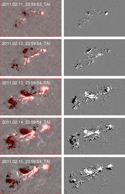
Figure 1.— Photospheric vector magnetograms (left) and maps of $J_{z}B_{z}$ (right) of the active region NOAA 11158 between 2011 February 11 to 15. The arrows indicate the transverse component of the magnetic field. Light (dark) shades indicate positive (negative) values of $B_{z}$ on the left and $J_{z}B_{z}$ on the right.

Figure 1 shows the photospheric vector magnetograms and the corresponding distribution of $h_{C}^{(z)}=J_{z}B_{z}$ from the vector magnetograms of that active region on different days. Here $J_{z}=\partial B_{y}/\partial x-\partial B_{x}/\partial y$ is proportional to the vertical component of the current density. The superscript ‘$(z)$’ on $h_{C}^{(z)}$ indicates that only the vertical contribution to the current helicity density are available.

We now consider the magnetic energy and helicity spectra for a field of view of $256^{\prime\prime}\times 256^{\prime\prime}$ (i.e., $512\times 512$ pixels). We average the resulting spectra from 600 vector magnetograms from 2011 February 12 to 16; see Figure 2. These are comparable with that of Zhang et al. (2014) except that the fluctuations in the calculation of individual samples are now reduced by the averaging. This provides a basic estimate of the spectra of magnetic energy and helicity of this active region.

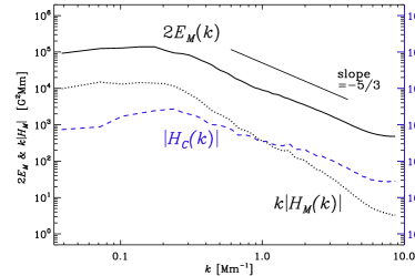
Figure 2.— $2E_{M}(k)$ (solid line), $k|H_{M}(k)|$ (dotted line), and $|H_{C}(k)|$ (dashed line) obtained by averaging over 600 vector magnetograms of active region NOAA 11158 from 2011 February 12 to 16.

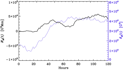
Figure 3.— Evolution of mean photospheric magnetic helicity density ${\cal H}_{M}(t)$ (solid line) and mean magnetic energy density ${\cal E}_{M}(t)$ (dotted line) of active region NOAA 11158.

Figure 3 shows the evolution of the mean magnetic helicity and energy densities for NOAA 11158, obtained by integrating over all $k$. It is found that the mean magnetic helicity and energy densities first increase and then continue to change as the active region develops. An intermediate decrease of the mean magnetic helicity density of the active region occurred on 2011 Feb. 14, while the mean magnetic energy density did not decrease. This shows that the mean magnetic helicity density in the active region does not always have a monotonous relationship with the mean magnetic energy density. This is also consistent with the trends found by Gao et al. (2012) for the current and kinetic helicity densities for NOAA 11158 using vector magnetograms and subsurface velocity fields.

According to the theory of hydromagnetic turbulence by Goldreich & Sridhar (1995), the magnetic energy spectrum has a power-law inertial range of $\propto k^{-\alpha}$, where the spectral index $\alpha$ is compatible with 5/3 (about 1.67) and is dominated by contributions from wave vectors in the direction that is perpendicular to the local magnetic field. These spectral properties were confirmed by Abramenko (2005) and Stenflo (2012) based on solar magnetic field observations.

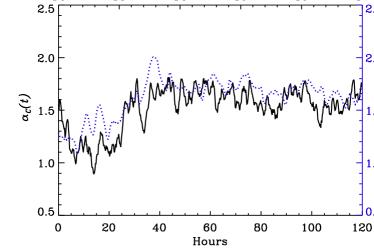
Figure 4.— Evolution of $\alpha_{C}$ (solid line) and $\alpha_{E}$ (dotted line) of active region NOAA 11158.

We estimate the spectral indices $\alpha_{i}$ with $i=E$ for magnetic energy and $i=C$ for current helicity within the wavenumber interval $1\,{\rm Mm}^{-1}<k<6\,{\rm Mm}^{-1}$, which should capture the spectral behavior in the inertial range of the turbulent magnetic field (we postpone the discussion of different wavenumber intervals to Section 5). Figure 4 shows the evolution of $\alpha_{i}$ for NOAA 11158. It is found that the minimum $\alpha_{E}$ is 1.1 and the maximum is 2.0. After 2011 February 13 as the active region became more developed, the mean value was about 1.65.

Under isotropic conditions, $H_{C}(k,t)$ is related to $H_{M}(k,t)$ via $H_{C}(k,t)\approx k^{2}H_{M}(k,t)$. Figure 4 shows the evolution of $\alpha_{C}$ for NOAA 11158. It is found that the minimum $\alpha_{C}$ is 0.9 and the maximum is 1.8. After 2011 February 13, the mean value was about 1.7. This implies that the value of $\alpha_{C}$ of this active region is of the order of 5/3 and consistent with our previous study (Zhang et al., 2014). Furthermore, the mean values of $\alpha_{E}$ and $\alpha_{C}$ of this active region at the solar surface are roughly consistent with a $k^{-5/3}$ power law. We also consider the spectrum $kH_{M}(k)$ and the corresponding spectral index $\alpha_{kH}$. If we had perfect power-law scaling, then $\alpha_{kH}=\alpha_{C}+1$, but the actual fits tend to give slightly larger values: its minimum value is 1.9, the maximum is 2.8, and the mean value is 2.65 as the active region develops.

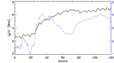
Figure 5.— Evolution of $l_{M}$ (solid line) and $r_{M}$ (dotted line) for the active region NOAA 11158.

The evolution of $l_{M}$ and $r_{M}$ in NOAA 11158 is shown in Figure 5. The average value of $r_{M}$ is about $+0.05$, while that of $l_{M}$ is about $6\,{\rm Mm}$ in the developed stage of the active region. These values are consistent with those quoted by Zhang et al. (2014). Being at $20^{\circ}$ southern heliographic latitude, the magnetic helicity was found to obey the expected hemispheric sign rule (positive in the south and negative in the north). It is found that the fractional magnetic helicity $r_{M}$ shows a relatively complex relationship with the temporal development of the active region and it shows a similar tendency with ${\cal H}_{M}$ in Figure 3.

3.2. Active Region NOAA 11515

To study the evolution of magnetic energy and helicity spectra in solar active regions, we have also analyzed HMI data from the active region NOAA 11515 from 2012 June 30 to July 6 at approximately $18\arcdeg$ southern latitude. The pixel resolution of magnetograms is about $0.5^{\prime\prime}$, and the field of view is $250^{\prime\prime}\times 150^{\prime\prime}$ in Figure 6. In our study about 840 vector magnetograms have been used.

Figure 6 shows the photospheric vector magnetograms and the corresponding distribution of $h_{C}^{(z)}=J_{z}B_{z}$ from the vector magnetograms of this active region on different days. It shows the spatial distribution of the magnetic field and the current helicity density of this active region at the solar surface.

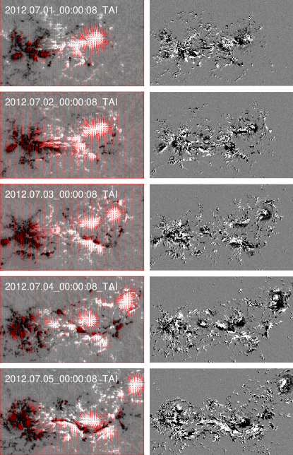
Figure 6.— Photospheric vector magnetograms (left) and maps of $J_{z}B_{z}$ (right) for the active region NOAA 11515 on 30 June – 4 July 2012. The arrows show the transverse component of the magnetic field. Light (dark) shades indicate positive (negative) values of $B_{z}$ on the left and $J_{z}B_{z}$ on the right.

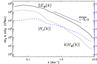
Figure 7.— Mean spectra of $2E_{M}(k)$ (solid line), $k|H_{M}(k)|$ (dotted line), and $|H_{C}(k)|$ (dashed line) obtained by averaging over 840 vector magnetograms of active region NOAA 11515 on 2012 June 30 – July 6.

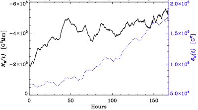
Figure 8.— Evolution of mean photospheric magnetic helicity density ${\cal H}_{M}(t)$ (solid line) and mean magnetic energy density ${\cal E}_{M}(t)$ (dotted line) of active region NOAA 11515. Note that the ordinate for ${\cal H}_{M}(t)$ shows negative values increasing upwards.

To analyze some basic properties of the magnetic energy and helicity spectra of this active region, we show in Figure 7 the averaged spectra that were inferred from the vector magnetograms from 2012 June 30 to July 6. These are comparable with the results of Zhang et al. (2014) and the average spectrum of NAOO 11158 in Figure 2. Comparing the two active regions NOAA 11158 and 11515, we find that the magnetic energy and helicity spectra are steeper in the latter case.

Figure 8 shows the evolution of mean magnetic helicity and energy densities of NOAA 11515, again obtained by integrating over all $k$. First note that ${\cal H}_{M}(t)$ is negative even though NOAA 11515 is located at a southern heliographic latitude. This is particularly surprising because $|{\cal H}_{M}(t)|$ is rather large, about 10 times larger than for NOAA 11158. It is therefore unlikely that the surprising sign is a consequence of fluctuations of a weak signal. The mean magnetic energy density is about three to five times larger than for NOAA 11158. Similar to NOAA 11158, there is an intermediate phase (50–100 hr after emergence) when ${\cal E}_{M}(t)$ still increases, but the increase of $|{\cal H}_{M}(t)|$ is interrupted by a phase of varying mean magnetic helicity density.

To understand the origin of the unconventional sign of helicity in this active region, we now consider the signed magnetic helicity spectra for 2012 July 3 where positive (negative) values are indicated by open (closed) symbols. It turns out that similar to NOAA 11158 where the signed magnetic helicity spectrum was shown in Figure 2 of Zhang et al. (2014), there is an intermediate range of $0.2\,{\rm Mm}^{-1}\leq k\leq 0.5\,{\rm Mm}^{-1}$, where $H_{M}(k)$ consistently shows a positive sign just as expected for the small-scale magnetic field in the southern hemisphere. However, for $k<0.2\,{\rm Mm}^{-1}$, the sign of $H_{M}(k)$ is in NOAA 11515 consistently negative (see Figure 9), which agrees with the sign expected for the large-scale field; see also Blackman & Brandenburg (2003). Again, this is not so different from the case of NOAA 11158, which also shows negative $H_{M}(k)$ for small $k$, but for NOAA 11515, the spectral slope is much larger, which is the reason for the dominance of the negative sign in the (integrated) mean magnetic helicity density.

By contrast, the current helicity, $\int k^{2}H_{M}(k,t)\,dk$, is dominated by the high wavenumber end of the spectrum. It is much noisier, so the hemispheric sign rule is often not obeyed. Furthermore, as shown by Xu et al. (2015), the isotropic approximation usually fails in such a case. While this must also be a concern for our present analysis, we should emphasize that the systematic sign changes that are a function of $k$ are certainly plausible and in agreement with theory (Blackman & Brandenburg, 2003).

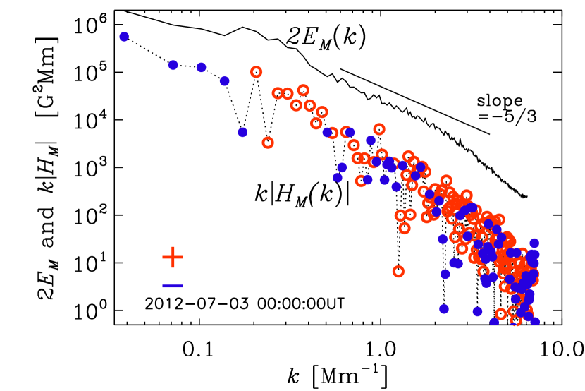
Figure 9.— $2E_{M}(k)$ (solid line) and $k|H_{M}(k)|$ (dotted line) for NOAA 11515 at 0:00:00 UT on 2012 July 3. Positive (negative) values of $H_{M}(k)$ are indicated by open (closed) symbols, respectively.

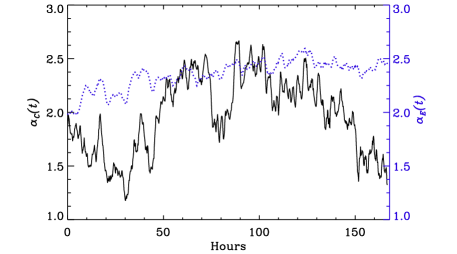
Figure 10.— Evolution of the spectral exponent $\alpha$ of the photospheric current helicity spectrum (solid line) and the magnetic energy spectrum (dotted line) of active region NOAA 11515.

Figure 10 shows the evolution of the mean spectral indices $\alpha_{E}$ and $\alpha_{C}$ for NOAA 11515 using the same wavenumber interval as before, i.e., $1\,{\rm Mm}^{-1}<k<6\,{\rm Mm}^{-1}$. The minimum of $\alpha_{C}$ is 1.2, the maximum is 2.7, and the mean value is about 2.0. The minimum of $\alpha_{E}$ is 2.0, the maximum is 2.6, and the mean value is about 2.4. These values are larger than those of NOAA 11158 and exceed the expected $5/3$ value.

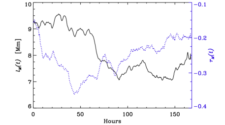
Figure 11.— Evolution of $l_{M}$ (solid line) and $r_{M}$ (dotted line) for active region NOAA 11515.

The evolution of $r_{M}$ and $l_{M}$ is shown in Figure 11. The average value of $r_{M}$ is about $-0.26$ while that of $l_{M}$ is about $8\,{\rm Mm}$ during the evolution of the active region. Thus, the strength of $r_{M}$ is about five times larger than it is for NOAA 11158. We see that the integral scale of the magnetic field decreases during the evolution of the active region even though the area of the active region increases. This is caused by a strong decrease of the mean magnetic energy density and could be interpreted as a saturation mechanism whereby this active region redistributes its rather large magnetic helicity over a larger area.

4. Magnetic Helicity and Energy Spectra of Active Regions with the Solar Cycle

Long-term statistical analyses of vector magnetograms at Huairou Solar Observing Station have been obtained over recent years (Bao & Zhang, 1998; Gao et al., 2008; Zhang et al., 2010), covering the epochs of cycles 22 and 23. These also provide an opportunity to analyze the evolution of the variation of the spectra of magnetic fields of active regions and the relationship with the solar activity cycle. The averaged effect of active regions is important for the theoretical interpretation and analysis of the solar cycle. Figure 12 shows the averaged spectra of $kH_{M}$ (dotted line), the current helicity $H_{c}$ (solid line), and the magnetic energy $E_{M}$ (dashed line) using 6629 Huairou vector magnetograms of the solar active regions observed from 1988 to 2005. The method is equivalent to that for individual active regions above. For consistency with the calculation of the long-term evolution of the magnetic field of active regions by means of a series of Huairou vector magnetograms, the spatial resolution of Huairou vector magnetograms has been downsampled to $2^{\prime\prime}\times 2^{\prime\prime}$ to reduce the influence of the different seeing conditions in the observations. Due to the relatively low spatial resolution, the spectra shown in Figure 12 become unreliable at large wavenumbers. To substantiate this, we compare the estimated energy spectra based solely on the horizontal fields as we did in Zhang et al. (2014).

$$2E_{M}^{(h)}(k,t)=4\pi k\,\mbox{Re}\left\langle\Gamma_{xx}+\Gamma_{yy}\right\rangle_{\phi_{k}},$$ (8)

with those based solely on the vertical ones,

$$2E_{M}^{(v)}(k,t)=4\pi k\,\mbox{Re}\left\langle\Gamma_{zz}\right\rangle_{\phi_{k}}.$$ (9)

Note the factor $4\pi$ on the right-hand sides of the two expressions above compared to only $2\pi$ in Equation (3). This accounts for why the two contributions should give an estimate of the full spectrum $2E_{M}(k,t)$. The shallow slope of the spectra of magnetic energy at high wavenumbers is an artifact of the lower resolution and is found to mainly concern the transverse components of the magnetic field. While this may in fact be physical at least for the Huairou vector magnetograms, the shallow spectral tails must be artifacts because they are not reproduced with HMI at a higher resolution. For more information about Huairou vector magnetograms we refer to the papers by Ai & Hu (1986), Su & Zhang (2004a, b), and Gao et al. (2008).

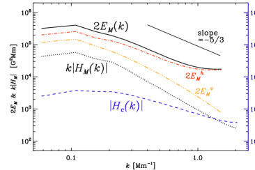
Figure 12.— Averaged magnetic energy spectrum (solid line) together with magnetic helicity (dotted line) and current helicity spectra (dashed line) obtained from 6629 Huairou vector magnetograms of solar active regions during 1988–2005. $2E_{M}^{(h)}(k)$ (red, dash-dotted) and $2E_{M}^{(v)}(k)$ (orange, dash-triple-dotted) are shown for comparison.

Table 1 Properties of active regions NOAA 11158 and 11515, and average properties from Huairou Solar Observing Station.

Time Latitude $\alpha_{E}$ $\alpha_{C}$ $r_{M}$ $l_{M}$ NOAA 11158 2011 February 12 to 17 $-13^{\circ}$     1.1 … 1.7 … 2.0 0.9 … 1.6 … 1.7 0.05 $6\,{\rm Mm}$ NOAA 11515 2012 June 30 to July 7 $-18^{\circ}$     2.0 … 2.4 … 2.6 1.2 … 2.0 … 2.7 $-0.26$ $8\,{\rm Mm}$ Huairou 1980 to 2005 —     1.6 1.0 $6$–$8\,{\rm Mm}$

We find similar magnetic helicity and energy spectra as for the individual active regions observed by HMI and the averaged ones inferred from the active regions observed at Huairou Solar Observing Station. The variation of the mean current helicity of active regions inferred from the Huairou vector magnetograms with sunspot butterfly diagrams has been studied by Zhang et al. (2010). It shows the same tendency as the variation of helicity and energy spectra for the individual active regions observed by HMI and the averaged ones inferred from the active regions observed at the Huairou Solar Observing Station; see Table LABEL:Tsummary for a more detailed comparison of the values quoted in Sections 3 and 4.

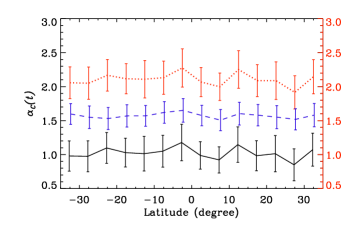
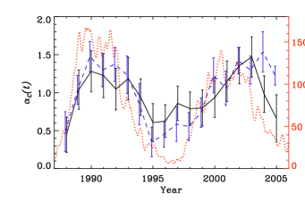
Figure 13.— Top: variation of $\alpha_{C}$ (solid line) and $\alpha_{E}$ (dashed line) with latitude (upper panel) and time (lower panel) inferred from 6629 Huairou vector magnetograms of solar active regions from 1988 to 2005. The dotted line shows $\alpha_{kH}$ in the top panel and sunspot number in the bottom panel. The error bars are $0.3\sigma$.

To analyze the evolution of the averaged magnetic helicity and energy spectra of solar active regions, Figure 13 shows the latitudinal and temporal dependence of $\alpha_{C}$ and $\alpha_{E}$ with the solar cycle in the spectral range of $0.2\,{\rm Mm}^{-1}<k<0.6\,{\rm Mm}^{-1}$. The slopes of the spectra do not change systematically with latitude when one averages the spectra of active regions for 1988 to 2005. This suggests that the underlying mechanism for producing these fields could be local small-scale dynamo action, which should operate equally at all latitudes. We emphasize that a small-scale dynamo is thought to operate independently of the large-scale dynamo, i.e., equally well on all latitudes. It is expected to produce scales that are smaller than those of the energy-carrying eddies or the energy-carrying magnetic structures $l_{M}$ (Brandenburg et al., 2012). This scale is of the order of a megameter and thus much smaller than the scale of active regions. In reality both dynamos are coupled, and the small-scale dynamo could even show a weak anticorrelation with the large-scale field (Karak & Brandenburg, 2016). Conversely, if we accept the local small-scale dynamo interpretation, the constancy of the slopes would demonstrate the robustness of our method in producing spectral slopes independent of seeing conditions and overall magnetic field strength, which would be largest at low latitudes. The mean spectral indices are $\alpha_{kH}\approx 2.1$, $\alpha_{C}\approx 1.0$, and $\alpha_{E}\approx 1.6$.

Figure 13 shows the temporal variation of the slopes of the spectra of magnetic energy and helicity of active regions between 1988 and 2000. These slopes show significant correlation with the sunspot number. High values occurred from 1990 to 1992 and from 2000 to 2003, while low values occurred during 1995. These are consistent with the periods of solar maximum and minimum, respectively. The correlation coefficient between the slopes of the current helicity spectra and sunspot numbers is 0.79 and that between the magnetic energy spectrum and sunspot number is 0.77. Note also that the mean magnetic energy density during the solar maximum is high. Furthermore, the maximum values of $\alpha_{E}$ and $\alpha_{C}$ tend to occur later than the maxima of the sunspot number. This is consistent with the observational result by Zhang et al. (2010) that the maximum in the butterfly diagram of the mean current helicity of active regions tends to be delayed compared with that of the sunspot number. A similar indication is that the complex magnetic configuration of active regions tends to occur in the decaying phase of solar cycle 23 (after 2002); see also Guo et al. (2010).

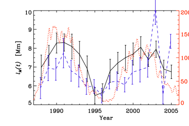
Figure 14.— Solid line shows the temporal evolution of the integral scale $l_{M}$ of the magnetic field and the dashed line shows that of the photospheric fractional magnetic helicity $|r_{M}|$ inferred by the 6629 Huairou vector magnetograms of the solar active regions during 1988–2005. The error bars are $0.3\sigma$. The dotted line shows the sunspot numbers.

Figure 14 shows the temporal evolution of the integral scale $l_{M}$ of the magnetic field of solar active regions inferred from 6629 Huairou vector magnetograms during 1988–2005. The correlation coefficient between the integral scale of the magnetic field, inferred from Equation (5) and the sunspot numbers, is 0.80. The average value of the integral scale of the magnetic field is about $8\,{\rm Mm}$ during solar maximum and $6\,{\rm Mm}$ during solar minimum for our calculated active regions. These dependencies are consistent with the finding that large-scale magnetic patterns of active regions tend to occur near solar maximum.

Figure 14 shows that the averaged absolute values, $\langle|r_{M}|\rangle$, of the photospheric fractional magnetic helicity of active regions obtained from Equation (7) correlate with the solar cycle as measured by the sunspot number except after 2003. The peak in the mean relative magnetic helicity during 2003–2005 is somewhat surprising, so we must ask about its physical significance. In this connection it is interesting to recall that based on analyses of MDI longitudinal magnetograms, thus using different data sets, Guo et al. (2010) reported an unusual magnetic field distribution dominated by a few very strong active regions during the declining phase of cycle 23. In support of the physical significance of the peak, it should be emphasized that there were several “superactive” regions such as NOAA 10484, 10486, and 10488, especially near the end of 2003. Of these, NOAA 10486 is generally associated with the famous Halloween flare of 2003 October 28 (e.g. Hady, 2009; Kazachenko et al., 2010). However, all three of these active regions showed high nonpotentiality (cf. Liu & Zhang, 2006; Zhou et al., 2007; Zhang et al., 2008). This is the reason for the high fractional magnetic helicity $|r_{M}|$ occurring statistically during this period.

5. Resolution dependence

In this study, the HMI and Huairou vector magnetograms have been used to estimate the spectra of magnetic energy and helicity of solar active regions. In addition, temporal changes of the magnetic energy spectra of active regions and the evolution with the solar cycle have been found. Since we use vector magnetograms of different spatial resolutions to analyze the evolution of the spectral distributions of magnetic energy at the different times, we now address the possible uncertainty regarding the relationship between the observational resolution of the magnetic field and the spectral shape at large wavenumbers. The lower spatial resolution of vector magnetograms of ground-based observations implies a source of error in the spectrum of the magnetic field at high wavenumbers.

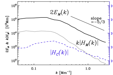
Figure 15.— Same as Figure 2, but with pixels compressed from 512$\times$512 to 128$\times$128.

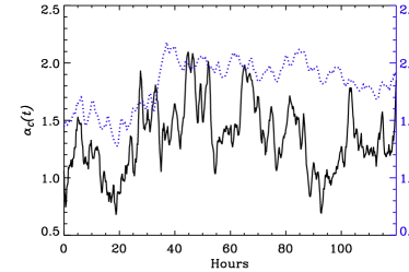
Figure 16.— Same as Figure 4, but with pixels compressed from 512$\times$512 to 128$\times$128.

To estimate the possible errors in the calculation of the magnetic spectrum due to the low spatial resolution of the observational magnetic fields by the Huairou vector magnetograms, Figure 15 shows the mean spectra of magnetic energy as well as magnetic and current helicity. Figure 16 shows the evolution of the spectral indices $\alpha_{C}$ and $\alpha_{E}$ for wavenumbers in the active region NOAA 11158, whose pixel size of the analyzed region of the HMI vector magnetograms have been downsampled from $512\times 512$ to $128\times 128$. The pixel resolution is $2^{\prime\prime}\times 2^{\prime\prime}$, which is almost the same as that of the Huairou vector magnetograms. The same tendency is found for the magnetic energy spectra as in Figure 2. The high noise in the timeseries of $\alpha_{C}$ and $\alpha_{E}$ in Figure 4 is now reduced. From 2011 February 12 to 16, the mean value of $\alpha_{E}$ is about 1.82 and that of $\alpha_{C}$ is about 1.34 for $0.4\,{\rm Mm}^{-1}<k<2.0\,{\rm Mm}^{-1}$, while the values obtained for the original resolution in Figure 4 are 1.52 and 1.62, respectively (the lower value of $\alpha_{E}$ given in Table LABEL:Tsummary is due to including the rapid growth during the emerging stage of the active region on 2011 February 12). For the detailed analysis we also have reversed the HMI vector magnetograms to Stokes parameters ($Q$, $U$, and $V$) in the approximation of the weak field with Gaussian smoothing for reducing to the forms of the lower spatial resolution, compressing them to the lower pixel resolution of the Stokes parameters, and then reverting to vector magnetograms again. We found almost the same tendency for the spectrum of magnetic fields such as shown in Figure 15, although the amplitudes of the slopes of the spectra of the magnetic fields changed slightly. We notice that we still cannot imitate the real case of the lower observational spatial resolution completely, such as the shallow slope of the spectra of magnetic energy at high wavenumbers in Figure 12. The difference with the degraded data implies that the resolution of the observational vector magnetograms might still be problematic in the diagnostics of the spectra of the magnetic field in the detail study. This may affect some of the analyses regarding the changes of the spectral slopes with the solar cycle when using the Huairou vector magnetograms, although one should keep in mind that our conclusions from the temporal variations are compatible with those found for individual active regions.

6. Conclusions

We have applied the technique of Zhang et al. (2014) to estimate the magnetic energy and helicity spectra using vector magnetogram data at the solar surface. We have made use of the assumption that the spectral two-point correlation tensor of the magnetic field can be approximated by its isotropic representation. In this paper we have analyzed the evolution of magnetic energy and helicity spectra in active regions and have also analyzed the changes during the solar cycle. Our major results are the following.

1. The values of $\alpha_{E}$ and $\alpha_{C}$ of solar active regions are of the order of $5/3$, although $\alpha_{C}$ is slightly smaller than $\alpha_{E}$, i.e., the current helicity spectrum is slightly shallower than the magnetic energy spectrum. We have also found a systematic change of $\alpha_{E}$ and $\alpha_{C}$ with the temporal development of active regions, which reflects their structural changes.

2. There is not necessarily an obvious relationship between the change of the photospheric fractional magnetic helicity $r_{M}$ and the integral scale of the magnetic field $l_{M}$ of individual active regions. Nevertheless, Figures 5 and 11 show that $r_{M}$ and $l_{M}$ tend to be correlated most of the time, which is also true for the cyclic variation shown in Figure 14. Looking at Equation 7, this might be somewhat surprising because it shows that $r_{M}$ and $l_{M}$ should be anticorrelated if ${\cal H}_{M}$ and ${\cal E}_{M}$ were constant. However, neither of them are constant and both show significant variations (see Figures 3 and 8).

3. We have found that there is a statistical correlation between the variation of the spectra of magnetic energy and helicity of solar active regions with the solar cycle. This implies that there is a trend for the characteristic scales and the intensity of the magnetic field of the active regions to increase statistically with the solar cycle.

4. Interestingly, even through the mean $\alpha_{E}$ and $\alpha_{C}$ of active regions vary with the cycle and increase with increasing mean magnetic energy density, they do not change with latitude even though the mean magnetic energy density does change with latitude.

   This suggests that the underlying magnetic field represents a part that is independent of the global cyclic magnetic field and possibly a signature of what is often referred to as local small-scale dynamo.

5. In NOAA 11515, where the fractional magnetic helicity is rather large (with a peak value of 35% and 26% on average), the integrated mean magnetic helicity density has the opposite sign of what is expected for its hemisphere. This is associated with a steepening of the magnetic helicity spectrum at large scales, therefore giving a preference to the contributions of the large-scale field whose magnetic helicity is indeed expected to have the opposite sign.

Values of $\alpha_{E}$ and $\alpha_{C}$ of the order of $5/3$ are roughly compatible with a Kolmogorov-like forward cascade (Kolmogorov, 1941; Obukhov, 1941), which is expected from the theory of nonhelical hydromagnetic turbulence when the magnetic field is moderately strong (Goldreich & Sridhar, 1995). However, for decaying turbulence Lee et al. (2010) found that the scaling depends on the field strength and takes on a shallower Iroshnikov–Kraichnan $k^{-3/2}$ spectrum (Iroshnikov, 1963; Kraichnan, 1965) for weaker fields and a steeper $k^{-2}$ weak-turbulence spectrum for stronger fields; see Brandenburg & Nordlund (2011) for the respective phenomenologies in the three cases. The steeper $k^{-2}$ spectrum has also recently been found in decaying turbulence simulations where the flow is driven entirely by the magnetic field (Brandenburg et al., 2015). It is thus tempting to associate the changes in the values of $\alpha_{E}$ and $\alpha_{C}$ with corresponding changes between these different scaling laws.

References

- Abramenko (2005) Abramenko, V. I. 2005, ApJ, 629, 1141
- Abramenko et al. (1997) Abramenko, V. I., Wang, T., & Yurchishin, V. B. 1997, SoPh, 174, 291
- Ai & Hu (1986) Ai, G. X., & Hu, Y. F. 1986, Publ. Beijing Astron. Obs., 8, 1
- Bao & Zhang (1998) Bao, S., & Zhang, H. 1998, ApJL, 496, L43
- Berger & Field (1984) Berger, M. A., & Field, G. B. 1984, JFM 147, 133
- Blackman & Brandenburg (2003) Blackman, E. G., & Brandenburg, A. 2003, ApJL, 584, L99
- Brandenburg & Subramanian (2005) Brandenburg, A., & Subramanian, K. 2005, A&A, 439, 835
- Brandenburg & Nordlund (2011) Brandenburg, A., & Nordlund, Å. 2011, Rep. Prog. Phys., 74, 046901
- Brandenburg et al. (2012) Brandenburg, A., Sokoloff, D., & Subramanian, K. 2012, Spa. Sci. Rev., 169, 123
- Brandenburg et al. (2011) Brandenburg, A., Subramanian, K., Balogh, A., & Goldstein, M. L. 2011, ApJ, 734, 9
- Brandenburg et al. (2015) Brandenburg, A., Kahniashvili, T., & Tevzadze, A. G. 2015, PhRvL, 114, 075001
- Chae (2001) Chae, J. 2001, ApJL, 560, L95
- Gao et al. (2008) Gao, Y., Su, J., Xu, H., & Zhang, H. 2008, MNRAS, 386, 1959
- Gao et al. (2012) Gao, Y., Zhao, J., & Zhang, H. 2012, ApJ, 761, L9
- Goldreich & Sridhar (1995) Goldreich, P., & Sridhar, S. 1995, ApJ, 438, 763
- Guo et al. (2010) Guo, J., Zhang, H. Q., Chumak, O. V., & Lin, J. B. 2010, MNRAS, 405, 111
- Hady (2009) Hady, A. A. 2009, J. Atmos. Solar-Terrestrial Phys., 71, 1711
- Hagino & Sakurai (2004) Hagino, M., & Sakurai, T.: 2004, Pub. Astron. Soc. Japan, 56, 831
- Iroshnikov (1963) Iroshnikov R. S. 1963, Astron Zh 40, 742 (English translation: 1964, Sov Astron 7, 566)
- Ji (1999) Ji, H. 1999, PhRvL, 83, 3198
- Karak & Brandenburg (2016) Karak, B. B., & Brandenburg, A. 2016, ApJ, 816, 28
- Kazachenko et al. (2010) Kazachenko, M. D., Canfield, R. C., Longcope, D. W., & Qiu, J. 2010, ApJ, 722, 1539
- Kleeorin & Ruzmaikin (1982) Kleeorin, N. I., & Ruzmaikin, A. A. 1982, Magnetohydrodynamics, 18, 116
- Kolmogorov (1941) Kolmogorov, A. N. 1941, Dokl. A N SSSR, 30, 299
- Kraichnan (1965) Kraichnan R. H. 1965, Phys Fluids, 8, 1385
- Lee et al. (2010) Lee, E., Brachet, M. E., Pouquet, A., Mininni, P. D., & Rosenberg, D. 2010, PhRvE, 81, 016318
- Liu & Zhang (2006) Liu, J. H., & Zhang, H. Q. 2006, Sol. Phys., 234, 21
- Matthaeus et al. (1982) Matthaeus, W. H., Goldstein, M. L., & Smith, C. 1982, PhRvL, 48, 1256
- Moffatt (1969) Moffatt, H. K. 1969, JFM, 35, 117
- Moffatt (1978) Moffatt, H. K. 1978, Magnetic Field Generation in Electrically Conducting Fluids, (Cambridge: Cambridge Univ. Press)
- Obukhov (1941) Obukhov, A. M. 1941, Dokl. A N SSSR, 32, 22
- Parker (1955) Parker, E. N. 1955, ApJ, 122, 293
- Pevtsov et al. (1994) Pevtsov, A. A., Canfield, R. C., & Metcalf, T. R. 1994, ApJL, 425, L117
- Pipin & Pevtsov (2014) Pipin, V. V., & Pevtsov, A. A. 2014, ApJ, 789, 21
- Seehafer (1990) Seehafer, N. 1990, SoPh, 125, 219
- Seehafer (1996) Seehafer, N. 1996, PhRvE, 53, 1283
- Steenbeck et al. (1966) Steenbeck, M., Krause, F., & Rädler, K.-H. 1966, Z. Naturforsch., 21a, 369
- Stenflo (2012) Stenflo, J. O. 2012, A&A, 541, A17
- Su & Zhang (2004a) Su, J. T., & Zhang, H. Q. 2004a, Chinese J. Astron. Astrophys., 4, 365
- Su & Zhang (2004b) Su, J. T., & Zhang, H. Q. 2004b, Solar Phys., 222, 17
- Taylor (1938) Taylor, G. I. 1938, Proc. Roy. Soc. London A, 164, 476
- Taylor (1986) Taylor, J. B. 1986, RvMP, 58, 741
- Tevzadze et al. (2012) Tevzadze, A. G., Kisslinger, L., Brandenburg, A., & Kahniashvili, T. 2012, ApJ, 759, 54
- Warnecke et al. (2011) Warnecke, J., Brandenburg, A., & Mitra, D. 2011, A&A, 534, A11
- Warnecke et al. (2012) Warnecke, J., Brandenburg, A., & Mitra, D. 2012, JSWJC, 2, A11
- Woltjer (1958) Woltjer, L. 1958, PNAS, 44, 833
- Xu et al. (2015) Xu, H., Stepanov, R., Kuzanyan, K., Sokoloff, D., Zhang, H., & Gao, Y. 2015, MNRAS, 454, 1921
- Yang & Zhang (2012) Yang, S., & Zhang, H. 2012, ApJ, 758, 61
- Zeldovich et al. (1983) Zeldovich, Y. B., Ruzmaikin, A. A., & Sokoloff, D. D, 1983, Magnetic fields in astrophysics, New York, Gordon and Breach
- Zhang et al. (2008) Zhang, Y., Liu, J. H., & Zhang, H. Q. 2008, Sol. Phys., 247, 39
- Zhang et al. (2010) Zhang, H., Sakurai, T., Pevtsov, A., Gao, Y., Xu, H., Sokoloff, D., & Kuzanyan, K. 2010, MNRAS, 402, L30
- Zhang & Yang (2013) Zhang, H., & Yang, S. 2013, ApJ, 763, 105
- Zhang et al. (2014) Zhang, H., Brandenburg A., & Sokoloff D. 2014, ApJ, 784, L45
- Zhou et al. (2007) Zhou, G., Wang, J., Wang, Y., & Zhang, Y. 2007, Sol. Phys., 244, 13