Quantifying Non-Markovianity with Temporal Steering

Abstract

Einstein-Podolsky-Rosen (EPR) steering is a type of quantum correlation which allows one to remotely prepare, or steer, the state of a distant quantum system. While EPR steering can be thought of as a purely spatial correlation there does exist a temporal analogue, in the form of single-system temporal steering. However, a precise quantification of such temporal steering has been lacking. Here we show that it can be measured, via semidefinite programming, with a temporal steerable weight, in direct analogy to the recently proposed EPR steerable weight. We find a useful property of the temporal steerable weight in that it is a non-increasing function under completely-positive trace-preserving maps and can be used to define a sufficient and practical measure of strong non-Markovianity.

Quantum entanglement, Einstein-Podolsky-Rosen (EPR) steering, and Bell non-locality are three of the most intriguing phenomena in quantum physics and, in varying degrees, are thought to act as resources; fuel that powers a range of quantum technologies. Entanglement Horodecki et al. (2009); Wiseman et al. (2007); Jones et al. (2007) comes in hand-in-hand with the complexity of quantum systems, and may be behind the potential speed-up of quantum computation. Bell non-locality and EPR steering are thought to be the driving power of quantum cryptography, and have both been recast in that language. For example, in a quantum key distribution scenario, two parties wish to generate a secret key using shared quantum states as a resource. If one party (Bob) trusts his own experimental apparatus but not that of the other party (Alice), a violation of a steering inequality Cavalcanti et al. (2009); Wiseman et al. (2007); Jones et al. (2007) can be used to certify that true quantum correlations exist between their shared states. In stricter terms, such a test proves to Bob that the correlations he observes between his measurement results and Alice’s cannot be described by a local hidden state model; his state is truly being influenced by Alice’s measurements in a non-local manner. As with entanglement, one quantify the amount of steering that is possible with a given shared state via a range of possible measures Jevtic et al. (2014); Kogias et al. (2015); He et al. (2015); Piani and Watrous (2015). Very recently, a powerful example of such a measure, the steerable weight, was proposed by Skrzypczyk et al. Skrzypczyk et al. (2014); Pusey (2013).

In EPR steering the notion of non-locality, via space-like separations between parties, plays an important role. If we relax this constraint, and consider time-like separation of measurement events, can the concept of steering still be used in a meaningful way? We can find inspiration in the fact that there do already exist other types of non-trivial temporal quantum correlations complementary to both Bell non-locality and entanglement. For the former, one of the most well-known examples is the Leggett-Garg (LG) inequality Leggett and Garg (1985), which can be used to test the assumption of “macroscopic realism”, in contrast to the non-local realism tested by Bell’s Inequality, and for which experimental violations have been observed in a large range of systems Palacios-Laloy et al. (2010); Knee et al. (2012); Emary et al. (2014). For the latter, motivated by the Choi-Jamiolkowski (CJ) isomorphism Jamiołkowski (1972), which equates the correlations in a bi-partite quantum system with two-time correlations of a single quantum system, the notion of temporal entanglement has been proposed in various forms Brukner et al. (2004); Fritz (2010); Olson and Ralph (2011, 2012); Sabín et al. (2012); Megidish et al. (2013); Fitzsimons et al. (2013). Returning to steering, the concept of temporal steering, and a temporal steering inequality, was recently introduced by Chen et al. Chen et al. (2014). Also inspired by the CJ isomorphism, they showed that, even without the assumption of non-locality, the concept of one party not trusting the earlier measurements made by another party delineates between certain classical and quantum correlations. Not only does this have direct practical applications in verifying a quantum channel for quantum key distribution (QKD), it was recently shown that temporal steering, like EPR steering Quintino et al. (2014); Uola et al. (2014), is intimately linked to the concepts of realism and joint measurability Li et al. (2014); Pusey (2015); Piani (2015); Karthik et al. (2015).

Still lacking however is a measure to quantify these “temporal steering” quantum correlations. Here, in analogy to the EPR steerable weight Skrzypczyk et al. (2014); Pusey (2013), we define the temporal-steerable-weight (temporal-SW) as a measure of temporal steering. We prove that the temporal-SW is non-increasing under a completely-positive trace-preserving (CPT) map and can be used to define a sufficient but not necessary measure of non-Markovianity. In the same way that the spatial steerable weight can be considered a measure of strong entanglement, since not every entangled state is steerable, we define the temporal-SW as a measure of strong non-Markovianity because it vanishes for weak non-Markovian process. (This is also in analogy to, e.g., the phenomenon of strong non-classicality, which can be detected and quantified by a weaker criterion of non-classicality Dodonov and Man’ko (2002); Arvind et al. (1997)). We show this by comparing the non-Markovianity measured by the temporal-SW to an existing entanglement-based measure Rivas et al. (2010), and find that it is, as expected, less-sensitive. However, the temporal-SW is, in principle, easier to implement experimentally, as it does not require the use of an ancilla, nor full process tomography. These results, together with with a few illustrative examples discussed mainly in the Supplementary Material Supplement , suggest that temporal steering can serve as a unique and useful quantum resource.

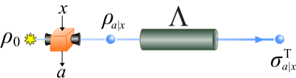
Figure 1: (Color online) Schematic diagram of temporal steering. In the beginning, Alice performs the measurement $F_{a|x}=M_{a|x}^{\dagger}M_{a|x}$ on an initial state $\rho_{0}$. Then, $\rho_{0}$ is mapped to $\rho_{a|x}$ and sent into a quantum channel $\Lambda$. Finally, Bob receives the assemblage $\{\sigma_{a|x}^{\text{T}}\}$ at time $t$.

Temporal steerable weight.— Now we introduce the concept of a temporal steerable weight in analogy to the spatial steerable weight introduced recently by Skrzypczyk et al. Skrzypczyk et al. (2014); Pusey (2013). In the standard (spatial) EPR steering scenario, Alice performs a POVM (positive-operator valued measure) measurement $F_{a|x}=M_{a|x}^{\dagger}M_{a|x}$, $\sum_{a}F_{a|x}=\openone$, on a state $\rho_{AB}$ shared with Bob and creates the assemblage $\{\sigma_{a|x}\}$, where $a$ is the measurement result and $x$ is the basis of the measurement. In defining a steering inequality, or a steerable weight, one assumes that Bob does not trust Alice, nor her experimental apparatus, and wishes to distinguish between true manipulation of his local state via quantum correlations and correlations that cannot be distinguished from some classical theory, typically a local hidden state model. In temporal steering, we also let Alice perform a POVM measurement $F_{a|x}=M_{a|x}^{\dagger}M_{a|x}$ but on a single system in an initial state $\rho_{0}$ at time $t=0$. After the measurement, the initial state is mapped to $\rho_{a|x}$ (see Fig. 1):

$$\rho_{0}\mapsto\rho_{a|x}=\frac{M_{a|x}\;\rho_{0}\;M_{a|x}^{\dagger}}{p(a|x)},$$ (1)

with the probability $p(a|x)=\text{tr}(M_{a|x}\rho_{0}M_{a|x}^{\dagger})$. After this initial measurement, the state $\rho_{a|x}$ is sent into a quantum channel $\Lambda$ for a time $t$. At time $t$, Bob receives the system and performs quantum tomography to obtain the state $\sigma_{a|x}$, i.e., $\Lambda(\rho_{a|x})=\sigma_{a|x}$. To mimic the unnormalized assemblage Skrzypczyk et al. (2014); Pusey (2013) in standard EPR-steering, we define the unnormalized states in temporal steering

$$\sigma_{a|x}^{\text{T}}\equiv p(a|x)\;\sigma_{a|x},$$ (2)

where the superscript T reminds one that the assemblage $\{\sigma_{a|x}^{\text{T}}\}$ is for temporal steering.

However, the quantum channel may be noisy, obliterating the influence of Alice’s measurement choice, or Alice’s measurement results could have been fabricated via classical strategies. In these cases, $\sigma_{a|x}^{\text{T}}$ may include, or be entirely described by, an unsteerable assemblage which we define as

$$\sigma_{a|x}^{\text{T,US}}=\sum_{\lambda}\;P(\lambda)\;P(a_{|x}|\lambda)\;\sigma_{\lambda}$$ (3)

where $\sum_{\lambda}P(\lambda)=1$. We have written the result $a$, conditional on the basis $x$, with a subscript notation $a_{|x}\equiv a|x$. In the EPR setting $\lambda$ represents a local hidden variable which determines the possible correlations between Alice’s and Bob’s measurement results from a source which obeys classical realism. As in that case, when Alice reveals her measurement results, Bob can update his knowledge of his state, as indicated by two equal forms (by applying the chain rule), $\sum_{\lambda}P(\lambda)P(a_{|x}|\lambda)\sigma_{\lambda}=\sum_{\lambda}P(a|x)P(\lambda|a_{|x})\sigma_{\lambda}.$ Then the unsteerable states are those states which obey the classical (realism) chain rule for Alice’s joint measurement results, as shown in a recent work on steering witnesses Li et al. (2014). No matter what happens during the transmission, Bob’s task is to check whether the assemblage he receives can be written in the hidden-state form [Eq. (3)] or not. If he can, this means the state Bob receives is independent of the basis $x$ Alice chooses to measure in. As mentioned above, this may be because the quantum channel is too noisy, such that the influence of Alice’s measurements is no longer discernable, or Alice’s measurement results could have been fabricated via classical strategies. On the other hand, if the assemblage Bob receives cannot be written in the form of Eq. (3), he is convinced that Alice has influenced his state by her choice of measurement. In this case, we call the assemblage Bob receives “temporally steerable” and is symbolized as $\{\sigma_{a|x}^{\text{T,S}}\}$.

To determine the steerable weight, one considers the overlap between the state Bob receives and the unsteerable assemblage, such that his state can be written as a mixture

$$\sigma_{a|x}^{\text{T}}=\mu\>\sigma_{a|x}^{\text{T,US}}+(1-\mu)\sigma_{a|x}^{\text{T,S}}.$$ (4)

To quantify the “steerability in time” for a given assemblage $\{\sigma_{a|x}^{\text{T}}\}$, one has to maximize $\mu$, i.e., maximize the proportion of $\sigma_{a|x}^{\text{T,US}}$. Then, the “temporal steerable weight” can be defined as $\text{TSW}=1-\mu^{\ast}$, in which $\mu^{\ast}$ is the maximum of $\mu$ and can be obtained from semidefinite programming Vandenberghe and Boyd (1996); Skrzypczyk et al. (2014); Pusey (2013):

$$\mu^{\ast}=~{}\text{max }{}{} \text{tr}\sum_{\lambda}\tilde{\sigma}_{\lambda}$$ (5)

subject to $$\sigma_{a|x}^{\text{T}}-\sum_{\lambda}D_{\lambda}(a|x)\tilde{\sigma}_{\lambda}\geq 0~{}~{} \forall~{}a,x$$

$$\tilde{\sigma}_{\lambda}\geq 0 \forall~{}\lambda,$$

where $\tilde{\sigma}_{\lambda}=\mu\sigma_{\lambda}$, and $D_{\lambda}(a|x)$ are the extremal deterministic values Skrzypczyk et al. (2014) of the conditional probability distributions $P(a_{|x}|\lambda)$. Equation (5), which is formulated as a semi-definite program (SDP), can be numerically implemented in various convex optimization packages, e.g., Refs. Grant and Boyd (2008); Andersen14 .

So far, the formalism is parallel to the standard EPR steerable weight Skrzypczyk et al. (2014). The primary difference is that $\{{\sigma}_{a|x}\}$ in Ref. Skrzypczyk et al. (2014) is created through the entanglement between Alice and Bob. Here, $\{\sigma_{a|x}^{\text{T}}\}$ is created through Alice’s measurement and the influence of the quantum channel $\Lambda$. In the Supplementary Material Supplement , we give an explicit pedagogical example of how to evaluate the temporal steerable weight.

Measure of non-Markovianity.— Now we apply the introduced temporal steering weight as a measure of non-Markovianity. Non-Markovianity is a term used to describe the situation when an environment surrounding a quantum system has memory of its past evolution. It is an important concept both because many natural and man-made quantum systems exist in a regime where the assumption of a Markovian (memory-less) environment fails, but also because it can lead to counter-intuitive results regarding the decay of quantum effects, particularly when the quantum system is strongly coupled to the surrounding environment. There has been a range of efforts at constructing measures of non-Markovianity, typically based on a scenario where the time evolution of a quantum system is analysed for non-Markovian properties. Arguably, the most popular measures of non-Markovianity were introduced in Refs. Breuer et al. (2009); Rivas et al. (2010). Recently, an attempt to classify these non-Markovianity measures in a unified framework was described in Ref. Chruściński and Maniscalco (2014). Useful for us here is the approach taken in  Breuer et al. (2009), which is based on observing the behavior of the trace distance between two quantum states. They derived a measure of non-Markovianity by noting that all CPT maps $\Phi$ are contractions of the trace distance metric, and a given dynamic processs is defined as Markovian if the map is divisible, i.e. $\Phi(\tau+t,0)=\Phi(\tau+t,t)\Phi(t,0)$, for all positive $t$ and $\tau$. These two properties lead to the monotonicity of the trace distance, and violations of this monotonicity indicate the occurrence of non-Markovian dynamics. In a similar way, below we prove that the temporal-SW of a system undergoing a CPT map is also a non-increasing function, i.e.,

$$\text{TSW}_{\rho}\geq\text{TSW}_{\Phi(\tau)\rho}$$ (6)

for a CPT map $\Phi(\tau)$. Together with the property of divisibility, one can conclude that the temporal-SW decreases monotonically under Markovian dynamics. Therefore our measure of non-Markovianity is defined by integrating the positive slope of the temporal-SW

$$\mathcal{N}_{\text{TSW}}\equiv\int_{\sigma_{\text{TSW}}>0}\!\!\!dt\,\sigma_{\text{TSW}}(t,\rho_{0},\Phi),$$ (7)

where $\sigma_{\text{TSW}}(t,\rho_{0},\Phi)=\frac{d}{dt}$TSW${}_{\Phi(t)\rho_{0}}$ is the rate of change of the temporal steerable weight. In the examples discussed in the Supplementary Material Supplement , we demonstrate explicitly how one can use this as a practical measure of strong non-Markovianity. Here we discuss only the following example.

Proof of the monotonicity of temporal-SW under Markovian dynamics.— First, we prove that the temporal-SW of a system undergoing a CPT map is a non-increasing function, as given by Eq. (6). To obtain the temporal-SW of a qubit at time $t_{1}$, one needs the quantity, $\sigma_{a|x}^{\text{T}}(t_{1})-\sum_{\lambda_{1}}D_{\lambda_{1}}(a|x)\tilde{\sigma}_{\lambda_{1}}$, in which the set $\{\tilde{\sigma}_{\lambda_{1}}\}$ is chosen to maximize Tr$(\sum_{\lambda_{1}}\tilde{\sigma}_{\lambda_{1}})$ at time $t_{1}$. Summing all the measurement outcomes $a$ and taking the trace, we have

$$\text{Tr}\left[\sum_{a}\sigma_{a|x}^{\text{T}}(t_{1})-\sum_{a}\sum_{\lambda_{1}}D_{\lambda_{1}}(a|x)\tilde{\sigma}_{\lambda_{1}}\right]$$ (8)

$$=\text{Tr}\left[\sum_{a}\sigma_{a|x}^{\text{T}}(t_{1})-\sum_{\lambda_{1}}\tilde{\sigma}_{\lambda_{1}}\right]=1-\mu_{1}^{\ast},$$

where we have used the properties $\sum_{a}D_{\lambda}(a|x)=1$, and Tr$\left[\sum_{a}\sigma_{a|x}^{\text{T}}(t_{1})\right]=1$. Similarly, to obtain the temporal-SW of the qubit at a later time $t_{2}=t_{1}+\tau$, one also has

$$\text{Tr}\left[\sum_{a}\sigma_{a|x}^{\text{T}}(t_{2})-\sum_{a}\sum_{\lambda_{2}}D_{\lambda_{2}}(a|x)\tilde{\sigma}_{\lambda_{2}}\right]=1-\mu_{2}^{\ast},$$ (9)

where $\{\tilde{\sigma}_{\lambda_{2}}\}$ is chosen to maximize Tr$(\sum_{\lambda_{2}}\tilde{\sigma}_{\lambda_{2}})$ at time $t_{2}$. One can also perform a CPT map $\Phi(\tau)$ to Eq. (8), giving

$$\text{Tr}\left[\sum_{a}\Phi(\tau)\sigma_{a|x}^{\text{T}}(t_{1})-\sum_{a}\sum_{\lambda_{1}}\Phi(\tau)D_{\lambda_{1}}(a|x)\tilde{\sigma}_{\lambda_{1}}\right]$$

$$\hskip 14.22636pt=\text{Tr}\left[\sum_{a}\sigma_{a|x}^{\text{T}}(t_{2})-\sum_{a}\sum_{\lambda_{1}}D_{\lambda_{1}}(a|x)(\Phi(\tau)\tilde{\sigma}_{\lambda_{1}})\right].$$ (10)

Since $\Phi(\tau)$ is a trace-preserving map, the value of Eq. (10) is still $1-\mu_{1}^{\ast}$. However, we know that the set $\{\tilde{\sigma}_{\lambda_{2}}\}$ is the optimal way to maximize Tr$(\sum_{\lambda_{2}}\tilde{\sigma}_{\lambda_{2}})$ at time $t_{2}$ for Eq. (9). Therefore, comparing Eq. (9) with Eq. (10) would give

$$1-\mu_{1}^{\ast}\geq 1-\mu_{2}^{\ast},$$ (11)

This proves the theorem given in Eq. (6). Employing the divisibility of Markovian dynamics leads to the monotonicity of the temporal-SW:

$$\text{TSW}\{\Phi(\tau+t,0)\sigma_{a|x}\} =\text{TSW}\{\Phi(\tau+t,t)\Phi(t,0)\sigma_{a|x}\}$$ (12)

$$\leq\text{TSW}\{\Phi(t,0)\sigma_{a|x}\}$$

An example of non-Markovianity of a spin-boson problem.— Exact solutions to the general spin-boson problem have applications in a huge range of systems, from quantum computing to physical chemistry and photosynthesis Ishizaki and Fleming (2009). Various techniques and methods exist to numerically acquire such solutions, one of the most powerful of which is the hierarchy equations of motion Tanimura (1990); Yoshitaka and Ryogo (1989). Here we use those equations to model a two-level system coupled to a bosonic environment or reservoir. The general Hamiltonian is written as

$$H_{\text{SB}}=\frac{E}{2}\sigma_{z}+\Delta\sigma_{x}+\sum_{\mathbf{k}}\omega_{\mathbf{k}}a_{\mathbf{k}}^{\dagger}a_{\mathbf{k}}+\sum_{\mathbf{k}}\sigma_{z}\otimes l_{\mathbf{k}}\left(a_{\mathbf{k}}^{\dagger}+a_{\mathbf{k}}\right),$$ (13)

where $\Delta$ is the two-level system tunneling amplitude, and $E$ is the two-level system splitting. The environment modes are described with creation ($a_{\mathbf{k}}^{\dagger}$) and annihilation operators ($a_{\mathbf{k}}$) with energy $\omega_{\mathbf{k}}$, which couple to the system, described by the Pauli operators $\sigma_{z}$ and $\sigma_{x}$, with strength $l_{\mathbf{k}}$. By assuming that the environment modes are well-described by a Drude-Lorentz spectral density, $J(\omega)=2\alpha\omega_{c}\frac{\omega}{\omega^{2}+\omega_{c}^{2}}$, where $\alpha$ is the system-reservoir coupling strength and $\omega_{c}$ is the bath cut-off frequency, we can exactly solve the dynamics of the two-level system (details can be found in Ref. Ishizaki and Fleming (2009); Tanimura (1990); Yoshitaka and Ryogo (1989)). We can then compare the non-Markovianity as measured via the temporal-SW to that given by the non-monotonic behavior of the entanglement, as given by the concurrence Horodecki et al. (2009), between the two-level system and an isolated ancilla Rivas et al. (2010). One important difference in the two approaches is that in the temporal-SW case there is no ancilla. In the ancilla case, the initial condition between the system and ancilla is that of a maximally-entangled state; to mimic that in the temporal-SW case we assume the two-level system is initially in a maximally-mixed state. We then evolve the entire system-reservoir equations of motion, using parameters relevant to energy transfer in photosynthesis Ishizaki and Fleming (2009), and plot both measures in Fig. 2.

For both measures we see similar behavior, particularly as a function of reservoir cut-off frequency and reservoir temperature. However, as a function of system-reservoir coupling, the entanglement measure has a larger window of detection. This may be attributed to the hierarchical relationship between EPR steering and entanglement. For example, Ref. Wiseman et al. (2007) has shown that EPR steerable states are a superset of Bell nonlocal states, and a subset of entangled states. This hierarchy links together these three different notions of quantum correlations. Therefore, the fact that the concurrence-based measure of non-Markovianity is more sensitive to the non-Markovianity than the temporal-SW measure seems linked, intuitively, to the notion that steering, in its EPR form, is a subset of entangled states. Also note that, the sharp features in both measures are typical, and arise because of the sudden vanishing and reappearance of both quantities in the temporal domain. Note that here, for consistency with Ref. Rivas et al. (2010), we plot $\mathcal{N}_{{\rm TSW}}$ and $\mathcal{N}_{{\rm C}}$ using

$$\mathcal{N}_{i}=\int_{t_{0}}^{t_{f}}\left|\frac{df_{i}[\rho(t)]}{dt}\right|dt+f_{i}[\rho(t_{f})]-f_{i}[\rho(t_{0})],$$ (14)

where for the temporal-SW measure $i={\rm TSW}$, the function $f_{i}[\rho(t)]$ is the temporal-SW at time $t$, while for the concurrence measure, $i={\rm C}$, the function $f_{i}[\rho(t)]$ is the concurrence between system and ancilla at time $t$. This definition for the integral differs from Eq. (7) by a trivial factor of $1/2$.

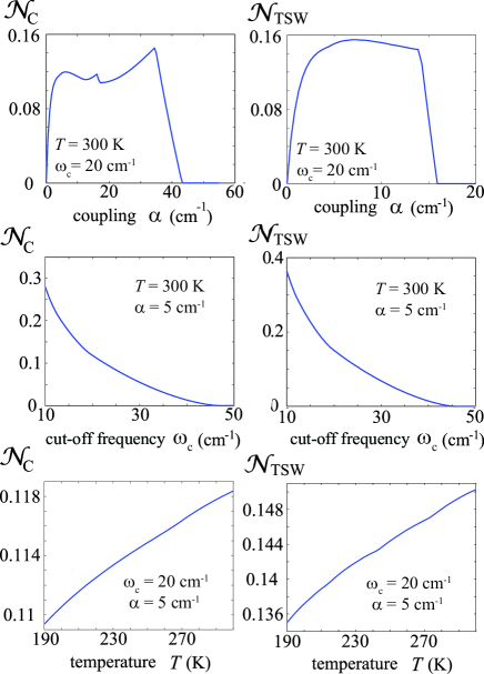
Figure 2: (Color online) The non-Markovianity measures, $\mathcal{N}_{\text{TSW}}$ (based on the temporal steerable weight) and $\mathcal{N}_{\text{C}}$ (based on the entanglement with an ancilla), as a function of system-reservoir coupling $\alpha$, reservoir cut-off frequency $\omega_{c}$ and temperature $T$, for a two-level system coupled to a bosonic reservoir with Drude-Lorentz spectral density. The system parameters are chosen to maximize the affect of the reservoir memory, with $E=0$ and $\Delta=100$cm^-1. The magnitude of these parameters are typical for excitation energy transfer in photosynthesis Ishizaki and Fleming (2009), where the memory effect and structure of the environment is thought to play an important role.

Conclusions.— To summarize, we have discussed the concepts of “temporal” steering and how this can be quantified in a similar way to that of the original spatial EPR-steering. We further proved that the temporal steerable weight decreases monotonically under a CPT map and can be used as a measure of non-Markovianity, suggesting that both forms of steering can act as a quantum resource, similar to entanglement. Finally we note that, in parallel, the temporal steerable weight has been recently implemented experimentally Bartkiewicz et al. (2015).

Acknowledgement.— The concept of a temporal steerable weight was developed here independently of the parallel work Bartkiewicz et al. (2015). S.-L. C. thanks H.-B. Chen for the discussion on quantum non-Markovianity. This work is supported partially by the National Center for Theoretical Sciences and Ministry of Science and Technology, Taiwan, grant number MOST 103-2112-M-006-017-MY4. A. M. is supported by the Polish National Science Centre under Grants DEC-2011/03/B/ST2/01903 and DEC-2011/02/A/ST2/00305. A. M. gratefully acknowledges a long-term fellowship from the Japan Society for the Promotion of Science (JSPS). F. N. is partially supported by the RIKEN iTHES Project, the MURI Center for Dynamic Magneto-Optics via the AFOSR award number FA9550-14-1-0040, the IMPACT program of JST, and a Grant-in-Aid for Scientific Research (A).

References

- Horodecki et al. (2009) R. Horodecki, P. Horodecki, M. Horodecki, and K. Horodecki, “Quantum entanglement,” Rev. Mod. Phys. 81, 865 (2009).
- Wiseman et al. (2007) H. M. Wiseman, S. J. Jones, and A. C. Doherty, “Steering, entanglement, nonlocality, and the Einstein-Podolsky-Rosen paradox,” Phys. Rev. Lett. 98, 140402 (2007).
- Jones et al. (2007) S. J. Jones, H. M. Wiseman, and A. C. Doherty, “Entanglement, einstein-podolsky-rosen correlations, bell nonlocality, and steering,” Phys. Rev. A 76, 052116 (2007).
- Cavalcanti et al. (2009) E. G. Cavalcanti, S. J. Jones, H. M. Wiseman, and M. D. Reid, “Experimental criteria for steering and the Einstein-Podolsky-Rosen paradox,” Phys. Rev. A 80, 032112 (2009).
- Jevtic et al. (2014) S. Jevtic, M. Pusey, D. Jennings, and T. Rudolph, “Quantum steering ellipsoids,” Phys. Rev. Lett. 113, 020402 (2014).
- Kogias et al. (2015) I. Kogias, A. R. Lee, S. Ragy, and G. Adesso, “Quantification of Gaussian quantum steering,” Phys. Rev. Lett. 114, 060403 (2015).
- He et al. (2015) Q. Y. He, Q. H. Gong, and M. D. Reid, “Classifying directional gaussian entanglement, einstein-podolsky-rosen steering, and discord,” Phys. Rev. Lett. 114, 060402 (2015).
- Piani and Watrous (2015) M. Piani and J. Watrous, “Necessary and sufficient quantum information characterization of Einstein-Podolsky-Rosen steering,” Phys. Rev. Lett. 114, 060404 (2015).
- Skrzypczyk et al. (2014) P. Skrzypczyk, M. Navascués, and D. Cavalcanti, “Quantifying Einstein-Podolsky-Rosen steering,” Phys. Rev. Lett. 112, 180404 (2014).
- Pusey (2013) M. F. Pusey, “Negativity and steering: A stronger Peres conjecture,” Phys. Rev. A 88, 032313 (2013).
- Leggett and Garg (1985) A. J. Leggett and A. Garg, “Quantum mechanics versus macroscopic realism: Is the flux there when nobody looks?” Phys. Rev. Lett. 54, 857 (1985).
- Palacios-Laloy et al. (2010) A. Palacios-Laloy, F. Mallet, F. Nguyen, P. Bertet, D. Vion, D. Esteve, and A. N. Korotkov, “Experimental violation of a Bell’s inequality in time with weak measurement,” Nat. Phys. 6, 442 (2010).
- Knee et al. (2012) G. C. Knee, S. Simmons, E. M. Gauger, J. J. L. Morton, H. Riemann, N. V. Abrosimov, P. Becker, H. J. Pohl, K. M. Itoh, M. L.W. Thewalt, G. A. D. Briggs, and S. C. Benjamin, “Violation of a Leggett-Garg inequality with ideal non-invasive measurements,” Nat. Commun. 3, 606 (2012).
- Emary et al. (2014) C. Emary, N. Lambert, and F. Nori, “Leggett-Garg inequalities,” Rep. Prog. Phys. 77, 016001 (2014).
- Jamiołkowski (1972) A. Jamiołkowski, “Linear transformations which preserve trace and positive semidefiniteness of operators,” Rep. Math. Phys. 3, 275 (1972).
- Brukner et al. (2004) Č. Brukner, S. Taylor, S. Cheung, and V. Vedral, “Quantum Entanglement in Time,” arXiv:quant-ph/0402127 (2004).
- Fritz (2010) T. Fritz, “Quantum correlations in the temporal Clauser-Horne-Shimony-Holt (CHSH) scenario,” New J. Phys. 12, 083055 (2010).
- Olson and Ralph (2011) S. J. Olson and T. C. Ralph, “Entanglement between the future and the past in the quantum vacuum,” Phys. Rev. Lett. 106, 110404 (2011).
- Olson and Ralph (2012) S. J. Olson and T. C. Ralph, “Extraction of timelike entanglement from the quantum vacuum,” Phys. Rev. A 85, 012306 (2012).
- Sabín et al. (2012) C. Sabín, B. Peropadre, M. del Rey, and E. Martín-Martínez, “Extracting past-future vacuum correlations using circuit qed,” Phys. Rev. Lett. 109, 033602 (2012).
- Megidish et al. (2013) E. Megidish, A. Halevy, T. Shacham, T. Dvir, L. Dovrat, and H. S. Eisenberg, “Entanglement swapping between photons that have never coexisted,” Phys. Rev. Lett. 110, 210403 (2013).
- Fitzsimons et al. (2013) J. Fitzsimons, J. Jones, and V. Vedral, “Quantum correlations which imply causation,” arXiv:1302.2731 (2013).
- Chen et al. (2014) Y.-N. Chen, C.-M. Li, N. Lambert, S.-L. Chen, Y. Ota, G.-Y. Chen, and F. Nori, “Temporal steering inequality,” Phys. Rev. A 89, 032112 (2014).
- Quintino et al. (2014) M. T. Quintino, T. Vértesi, and N. Brunner, “Joint measurability, Einstein-Podolsky-Rosen steering, and Bell nonlocality,” Phys. Rev. Lett. 113, 160402 (2014).
- Uola et al. (2014) R. Uola, T. Moroder, and O. Gühne, “Joint measurability of generalized measurements implies classicality,” Phys. Rev. Lett. 113, 160403 (2014).
- Li et al. (2014) C.-M. Li, Y.-N. Chen, N. Lambert, C.-Y. Chiu, and F. Nori, “Certifying single-system steering for quantum-information processing,” Phys. Rev. A 92, 062310 (2015).
- Pusey (2015) M. F. Pusey, “Verifying the quantumness of a channel with an untrusted device,” J. Opt. Soc. Am. B 32, A56 (2015).
- Piani (2015) M. Piani, “Channel steering,” J. Opt. Soc. Am. B 32, A1 (2015).
- Karthik et al. (2015) H. S. Karthik, J. Prabhu Tej, A. R. Usha Devi, and A. K. Rajagopal, “Joint measurability and temporal steering,” J. Opt. Soc. Am. B 32, A34 (2015).
- Dodonov and Man’ko (2002) V. V. Dodonov and V. I. Man’ko, eds., Theory of Nonclassical States of Light (Taylor & Francis, London, 2002).
- Arvind et al. (1997) Arvind, N. Mukunda, and R. Simon, “Gaussian-wigner distributions and hierarchies of nonclassical states in quantum optics: The single-mode case,” Phys. Rev. A 56, 5042 (1997).
- Rivas et al. (2010) A. Rivas, S. F. Huelga, and M. B. Plenio, “Entanglement and non-Markovianity of quantum evolutions,” Phys. Rev. Lett. 105, 050403 (2010).
- (33) For a few illustrative examples, see Supplemental Material [url], which includes Refs. Laine et al. (2010); Boyd04 .
- Laine et al. (2010) E.-M. Laine, J. Piilo, and H.-P. Breuer, “Measure for the non-Markovianity of quantum processes,” Phys. Rev. A 81, 062115 (2010).
- (35) S. Boyd and L. Vandenberghe, Convex Optimization (Cambridge University Press, Cambridge, 2004).
- Vandenberghe and Boyd (1996) L. Vandenberghe and S. Boyd, “Semidefinite programming,” SIAM Review 38, 49 (1996).
- Grant and Boyd (2008) M. Grant and S. Boyd, “CVX: Matlab software for disciplined convex programming,” (2008).
- (38) M. Andersen, J. Dahl, and K. Vandenberghe, CVXOPT: Python software for convex optimization (2014). url:http://cvxopt.org/.
- Breuer et al. (2009) H.-P. Breuer, E.-M. Laine, and J. Piilo, “Measure for the degree of non-Markovian behavior of quantum processes in open systems,” Phys. Rev. Lett. 103, 210401 (2009).
- Chruściński and Maniscalco (2014) D. Chruściński and S. Maniscalco, “Degree of non-markovianity of quantum evolution,” Phys. Rev. Lett. 112, 120404 (2014).
- Ishizaki and Fleming (2009) A. Ishizaki and G. R. Fleming, “Theoretical examination of quantum coherence in a photosynthetic system at physiological temperature,” J. Chem. Phys. 130, 234111 (2009).
- Tanimura (1990) Y. Tanimura, “Nonperturbative expansion method for a quantum system coupled to a harmonic-oscillator bath,” Phys. Rev. A 41, 6676 (1990).
- Yoshitaka and Ryogo (1989) T. Yoshitaka and K. Ryogo, “Time evolution of a quantum system in contact with a nearly Gaussian-Markoffian noise bath,” J. Phys. Soc. Japan 58, 101 (1989).
- Bartkiewicz et al. (2015) K. Bartkiewicz, A. Černoch, K. Lemr, A. Miranowicz, and F. Nori, “Experimental temporal steering and security of quantum key distribution with mutually-unbiased bases,” arxiv:1503.00612 (2015).