Abnormal Synchronizing Path of Delay-coupled Chaotic Oscillators on the Edge of Stability

Abstract

In this paper, the transition of synchronizing path of delay-coupled chaotic oscillators in a scale-free network is highlighted. Mainly, through the critical transmission delay makes chaotic oscillators be coupled on the edge of stability, we find that the transition of synchronizing path is abnormal, which is characterized by the following evidences: (a) synchronization process starts with low-degree rather than high-degree ones; (b) the high-degree nodes don’t undertake the role of hub; (c) the synchronized subnetworks show a poor small-world property as a result of hubs absence; (d) the clustering synchronization behavior emerges even community structure is absent in the scale-free network. This abnormal synchronizing path suggests that the diverse synchronization behaviors occur in the same topology, which implies that the relationship between dynamics and structure of network is much more complicated than the common sense that the structure is the foundation of dynamics. Moreover, it also reveals the potential connection from the transition of synchronization behavior to disorder in real complex networks, e.g. Alzheimer disease

1 Introduction

Synchronization, which is referred to as the uniform activities of interacting units, is ubiquitous in nature and plays an important role in physics, biology, sociology, technology and neural systems [1, 2]. Generally, real-world systems are often represented by networks, of which the nodes are units and edges indicate their interactions [3, 4, 5, 6]. A networked system consisting of $N$ coupled oscillators (i.e., nodes) thus can be simply described by $\dot{\mathbf{x}}_{i}=\mathbf{F}(\mathbf{x}_{i})-c\sum_{i}l_{ij}\mathbf{H}(\mathbf{x}_{j})$, where $\mathbf{x}_{i}$ describes the the $m$-dimensional state of node $i$ ($i=1,2,...,N$), $\mathbf{F}$ indicates nodes’ dynamics, $c$ and $F$ are the coupling strength and function, and $\mathbf{L}=(l_{ij})_{N\times N}$ is the Laplacian matrix of network. It reaches synchronization if all oscillators satisfy $\mathbf{x}_{1}(t)\equiv\mathbf{x}_{2}(t)\equiv...\equiv\mathbf{x}_{N}(t)$.

The synchronizability of network usually emphasizes whether its synchronization is achievable. Pecora and Carroll [7] varied coupling strength and firstly unraveled that the synchronizability of network could be evaluated by the eigenratio $\lambda_{max}/\lambda_{2}$, where $\lambda_{max}$ and $\lambda_{2}$ were the maximum and minimum non-trivial eigenvalue of $\mathbf{L}$. The smaller the eigenratio is, the stronger synchronizability the network has, and vise versa. Following this pioneering work, many researches have comprehensive investigated how to improve synchronizability of network via edge betweenness [8], topology modification [9, 10], optimization [11, 12, 13], adaptive evolution [14], and so on. Besides the network structure, Li and Chen [15] found that transmission delay between oscillators also influenced synchronizability of network deeply due to the signals traveling in limited speed, such as neural oscillators [16].

Moreover, the temporal characteristics shown in synchronization process can provide more information of the structure and function of system. For examples, the temporal correlations between interacting neural oscillators represent the clustering structure of coupling topology [17, 18], and clustering synchronization has been applied in community detection [19, 20] and data clustering [21, 22]. It is also worthy to discuss one of the most attractive temporal characteristics, synchronizing path that describes how the synchronized state diffuses to whole network. Gómez-Gardeñes et al [23] studied the synchronization path based on Kuramoto model, and showed it behave difference from Barabási-Albert scale-free (BA) network to Erdös-Rényi random (ER) network. Especially, the high-degree nodes in BA network were more likely to be synchronized into the central cluster than low-degree ones. And, Stout et al [24] proved that the synchronizing path observed in Ref. [23] was robust to increasing oscillator number and changing the distribution function of the Kuramoto oscillators’ natural frequencies. Recently, Zhou et.al [25] studied the influence of the mixing pattern on synchronizing path and found that the disassortative BA networks synchronize via a merging process rather than the typical growth process on BA network.

In this paper, we mainly investigate how the transmission delay affects the synchronization of chaotic oscillators. Based on a BA network consisting of Rössler oscillators, two distinct types of synchronizing paths are found via controlling transmission delay. Especially, when transmission delay achieves a critical value, the synchronizing path shows abnormal evidences that (a) these low-degree nodes rather than high-degree ones firstly synchronized, (b) the high-degree nodes no longer act as hubs in synchronization process because they join the largest synchronized cluster very late, (c) the largest synchronized cluster show poor small-world property as a result of absent hubs, (d) the clustering synchronization behaviors appears even the BA network is in absence of community. These features make the abnormal synchronizing path on the edge of stability (i.e., critical transmission delay) obviously differ from that on the stable region, and also reveal the disagreement between structure and dynamics of network. Meanwhile, this transition of synchronizing path suggests that the same topology can display diverse synchronization behaviors, which may provide a deep insight to understand the Alzheimer disease.

2 Synchronization of Delay-coupled Chaotic Oscillators

The network consisting of $N$ delay-coupled oscillators is represented by

$$\dot{\mathbf{x}}_{i}(t)=\mathbf{F}[\mathbf{x}_{i}(t)]-c\Sigma^{N}_{j=1}l_{ij}\mathbf{H}[\mathbf{x}_{j}(t-\tau)],$$ (1)

where $\tau$ is the transmission delay, $c$ is the coupling strength, and $l_{ij}$ is the entry of $\mathbf{L}$ at the $i$-th line and $j$-th column. The coupling function $\mathbf{H(\mathbf{x})}$ is set in the linear form as $\mathbf{H(\mathbf{x})}=\mathbf{x}$. As proved in Ref. [26], there exists a critical transmission delay $\tau_{c}$ that the synchronization is stable (unstable) if $\tau<\tau_{c}$($\tau>\tau_{c}$). The synchronization error $W(t)$ is adopted to measure the degree of synchronization,

$$W(t)=\frac{1}{N}\Sigma_{i=1}^{N}|\mathbf{x}_{i}-\langle\mathbf{x}_{i}\rangle|^{2},$$ (2)

where $\langle...\rangle$ denotes averaging over all nodes. Then the logarithmic synchronizing speed is defined as

$$\mu(t)=-\frac{d\ln[W(t)]}{dt}.$$ (3)

Positive synchronizing speed means that the $W(t)$ vanishes and the synchronization is stable. Thus, the critical transmission delay can be found by checking the sign of synchronizing speeds.

The Rössler oscillator is chosen for the numeric estimation of synchronous behaviors, which reads as

$$\left\{\begin{aligned} &\dot{x}_{i1}=-x_{i2}-x_{i3},\\ &\dot{x}_{i2}=x_{i1}+0.2x_{i2},\\ &\dot{x}_{i3}=0.2+x_{i3}(x_{i1}-12).\\ \end{aligned}\right.$$ (4)

We use the Barabási-Albert (BA) model with node number $N=1000$ and mean degree $\bar{k}=10$ as the coupling topology and set coupling strength as $c=3$. The synchronization processes are carried out by fourth-order Ronge-Kutta method with fixed step $\delta t=1.0\times 10^{-4}$.

The synchronizing speeds with varying transmission delays are obtained by the first-order polynomial fitting of $ln[W(t)]$ after transient time of $10^{4}$ steps, which is shown in Fig. 1. It can be seen that the critical transmission delay is around $4.2\times 10^{-3}$. Then the synchronization with $\tau_{c}=4.2\times 10^{-3}$ act as an example of collective dynamics on the edge of stability and the one with $\tau=2.0\times 10^{-3}$ as that in the stable region to be compared with. Both of the temporal evolutions of $W(t)$ are shown in the inset plot of Fig .1. In order to study the temporal synchronization behavior, we capture a serial snapshots of network state. Since the $W(t)$ for critical transmission delay is the combination of a decreasing trend and periodic fluctuation (see Fig. 1), the times series $[t_{1},t_{2},...,t_{m}]$ are chosen as $W(t_{i})$ is the local maximum. For simplicity to compare the temporal synchronization behaviors, snapshots of synchronization process in the stable region, whose synchronization degree is indicated by $W^{\prime}(t)$, are chosen at the time series $[t^{\prime}_{1},t^{\prime}_{2},...,t^{\prime}_{m}]$ satisfying $W(t_{i})=W^{\prime}(t^{\prime}_{i})$. Only snapshots of $t_{i}$ after $3\times 10^{4}$ steps are considered to avoid the disturbance in the transient time. Total $M=356$ snapshots are selected in each synchronization, part of which is shown in Fig. 1.

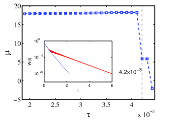
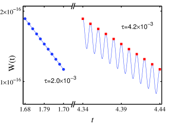
Figure 1: (Color online) (a) The logarithmic synchronizing speed of delay-coupled oscillates. The critical transmission delay $\tau_{c}=4.2\times 10^{-3}$ is marked by the dashed line. For the inner plot, it gives temporal evolutions of $W(t)$ when $\tau$ is $2.0\times 10^{-3}$ (blue line) and $4.3\times 10^{-3}$ (red line). (b) Part of the snapshots of synchronization process. $\blacksquare$ indicates snapshot of synchronization on the edge of stability and $\bullet$ describes the corresponding one of synchronization on the stable region, which shows the same synchronization error. Note the break in $x$-axis.

3 Synchronizing Path on the Edge of Stability

According to the method in Ref. [23], we investigate the synchronizing path via examining how the synchronized clusters grow in the snapshots. The synchronized clusters are extracted as follows. The edge linking node $i$ and $j$ is weighted by the Euclidean distance between the nodes

$$w_{\{i,j\}\in E}=|\mathbf{x}_{i}-\mathbf{x}_{j}|^{2}.$$ (5)

Then a threshold $T$ is set and the edges associated to weights less than the threshold are preserved to form a new network for each snapshot. In this new networks, two connected nodes are considered as synchronized. The largest synchronized cluster is defined as the giant component (GC) of the new network. Here we choose the synchronization error of the last snapshot $W(t_{M})=W^{\prime}(t^{\prime}_{M})$ as the threshold. The percents $p(t)$ of preserved edges and sizes of GCs $S(t)$ as a function of synchronization error $W(t)$ for two synchronization processes are show in Fig. 2 and 2, respectively. Note that the decreasing order in $x$-axis of both figures is in correspondence to the increase of time and decrease of synchronization error. One can see that at the same degree of synchronization, more edges are preserved and the GCs are larger in the snapshots of synchronization with the critical transmission delay than those in the snapshots of synchronization on the stable region. This result suggests that at the same degree of synchronization the network is more synchronized on the edge of stability and imply a different synchronizing path.

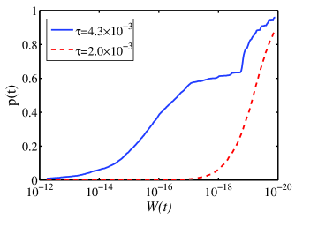
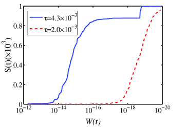
Figure 2: (Color online) (a) The percent of preserved edges. (b) The size of GC. Both of them imply the difference of synchronizing path between these two synchronization processes. Note that in both figures, the decreasing order in $x$-axis indicates the increase of time and decrease of synchronization error.

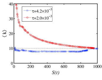
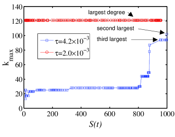
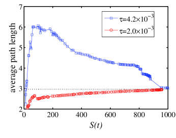
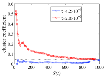
Figure 3: (Color online) (a) The mean degree $\langle k\rangle$ of nodes in the GC, (b) The largest degree $k_{max}$ of nodes in the GC, (c) the average path length of GC, and (d) the cluster coefficient of GC as function of its size $S(t)$. The dotted line indicates the mean degree, largest degree, average path length and cluster coefficient of network in (a), (b), (c) and (d), respectively. Note that in all figures, the increasing order in $x$-axis indicates the increase of time and decrease of synchronization error.

It has been observed that nodes’ degrees are tightly connected to the synchronization process, e.g. phase synchronization starts at high-degree nodes [23] and explosive synchronization emergences if the natural frequencies of oscillators depend on their degrees [27, 28]. Naturally, we examine the degrees (corresponding to BA network) of nodes in the GC to give a details of synchronizing path. In Fig. 3, it shows the mean degree $\langle k\rangle$ of nodes in the GC as function of its size $S(t)$. The referred baseline is the mean degree $\bar{k}=10$ of the BA network. Concretely, when the size of GC is small, the mean degrees of the synchronization on the stable region are much higher than $\bar{k}=10$, which suggests that the synchronization starts at the high-degree nodes. As the size of GC grows, the the mean degree decreases to $\bar{k}=10$ because of the join of low-degree nodes. on the contrary, the synchronization on the edge of stability starts with some low-degree nodes since the mean degree is around $\bar{k}$ at the beginning, then the mean degree further decreases to smaller than $\bar{k}$ because more low-degree nodes join. It starts to increase till the GC is relevantly large which implies that the high-degree nodes join the GC very late. To further determine the result, we present the largest degree $k_{max}$ in the GC as a function of $S(t)$, shown in Fig. 3. It can be seen that the largest degree $K_{max}=121$ of the BA network join the GC at the very beginning for transmission delay $\tau=2.0\times 10^{-3}$, while it is isolated for critical transmission delay. In the BA network, high-degree nodes act as structural hubs and play an important role in dynamic processes such as pinning control [29] and synchronization [30]. However, they lost their roles as hubs in the abnormal synchronizing path, which suggests the disagreement between structure and dynamics of network. As it’s unambiguously agreed that many networks realize their functions via dynamical processes, the disagreement will lead to disorder of system.

As a result of the hubs’ absence, the GCs in the synchronization on the edge of stability display poor small-world properties. As shown in Figs.3 and 3, it is characterized by the larger average path lengths and lower cluster coefficients compared with their baselines of the BA network. However, for the synchronization on the stable region, the average path lengths are shorter and cluster coefficients are higher in the normal synchronizing path. This variation of small-world property is also observed in the collective dynamics of real complex systems, e.g. the brain, which usually suggests disorders in the neural activities. In an study based on fMRI of Alzheimer disease (AD), clustering was significantly reduced in brain functional networks and the loss of small-world property is able to discriminate AD patients from age-matched comparison subjects with high specificity and sensitivity [31]. In another EEG study of AD, path lengths in brain functional networks constructed by $\beta$-band ($15-35$ Hz) waves were significantly increased in AD patients [32]. Therefore, the observation of small-world properties further suggests the abnormal synchronizing path is potentially related to disorders in real complex systems.

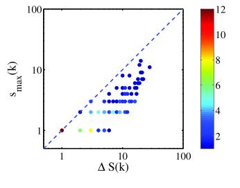
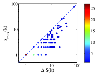
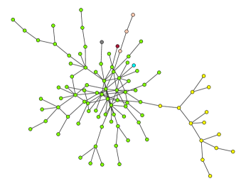
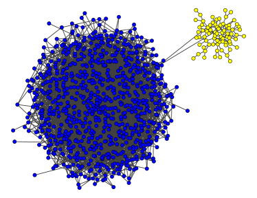
Figure 4: (Color online) (a) $\Delta S(k)$ vs. $s_{max}$ of normal synchronizing path (b) $\Delta S(k)$ vs. $s_{max}(k)$ of abnormal synchronizing path (c) the growth of GC in normal synchronizing path, $\Delta S(k)=20$, $s_{max}(k)=14$ and $k=259$. The size of GC increases from $74$ to $94$. (d) the growth of GC in abnormal synchronizing path, $\Delta S(k)=s_{max}(k)=76$ and $k=301$. The size of GC increases from $878$ to $954$.

To investigate how the GCs diffuse to the whole network in synchronization with transmission delay, we examine whether the nodes newly joining the GC at each snapshot are isolated ones or in synchronized clusters at the previous snapshot. Assuming $V(k)$ is the set of the nodes newly joining the GC at the $k$-th snapshot and $V^{\prime}(k,c_{i})$ is the subset of $V(k)$ containing the nodes that belong to synchronized clusters labeled by $c_{i}$ at the $(k-1)$th snapshot. Denote the number of newly joined nodes as $\Delta S(k)=|V(k)|$ and the maximum size of subsets as $s_{max}(k)=\max_{i}|V^{\prime}(k,c_{i})|$. The points of ($\Delta S(k)$,$s_{max}(k)$) of two synchronizing paths are shown in Fig. 4 and 4 respectively. Color of points indicates their number of occurrence. Small ($\Delta S(k)$, $s_{max}(k)$) pairs represent the nodes connect to GC as isolated ones, which takes most parts of ($\Delta S(k)$, $s_{max}(k)$) pairs in normal synchronizing path (see Fig. 4). High $\Delta S(k)$ and $\Delta S(k)\approx s_{max}(k)$ imply the nodes join the GC as one synchronized cluster, which can be found in the abnormal synchronizing path (see Fig. 4). Fig. 4 and 4 respectively show two examples of GC’s growth , whose $\Delta S(k)$ and $s_{max}(k)$ are both large, in normal and abnormal synchronizing paths via drawing network using Pajek [33]. In both figures, the separated clusters in the previous snapshot are indicated by different colors. The clustering synchronization behavior is clearly demonstrated in Fig. 4, though the communities don’t exist in the BA network. The result further supports the disagreement between structure and dynamics in abnormal synchronizing path.

4 Conclusion

In summary, we have shown that transmission delay can deeply influence the temporal synchronization behavior. Even the synchronization processes are all exponential convergence on the edge of stability and on the stable region, they display completely different synchronizing paths. In the synchronization with critical transmission delay, the high-degree nodes loss their roles as hubs in the collective dynamics. As a result, the synchronized part of network displays poor small-world properties in the abnormal synchronizing path. In further, a detailed investigation of the growth of the largest synchronized clusters suggests that the clustering synchronization behaviors are contained in abnormal synchronizing path though the communities don’t exist in BA model. Our work demonstrates that the same network structure can display different dynamic behaviors with varying transmission delay, and the transition of synchronizing path leads to disagreement between structure and dynamics, which is probably related to the disorder of real complex systems, e.g. the disease of human brain.

5 Acknowledgements

This work is jointly supported by the National Nature Science Foundation of China (Nos. 60974079 and 61004102), China Postdoctoral Science Foundation (No. 2013M541840), and the Fundamental Research Funds for the Central Universities (No. ZYGX2012J075)

References

- [1] A. Pikovsky, M. Rosenblum, J. Kurths, Synchronization: A Universal Concept in Nonlinear Science, Cambridge University Press, New York, (2002).
- [2] A. Arenas, A. Díaz-Guilera, J. Kurths, Y. Moreno, C. Zhou, Phys. Rep. 469 (2008) 93.
- [3] D. J. Watts, S. H. Strogatz, Nature, 393 (1998) 440.
- [4] R. Albert, A. L. Barabási, Rev. Mod. Phys. 74 (2002) 47.
- [5] M. E. J. Newman, SIAM Rev. 45 (2003) 167.
- [6] S. Boccaletti, V. Latora, Y. Moreno, M. Chavez, D. U. Hwang, Phys. Rep. 424 (2006) 175.
- [7] L. M. Pecora, T. L. Carroll, Phys. Rev. Lett. 80 (1998) 2109.
- [8] M. Chavez, D. U. Hwang, A. Amann, H. G. E. Hentschel, S. Boccaletti, Phys. Rev. Lett. 94 (2005) 218701.
- [9] M. Zhao, T. Zhou, B. H. Wang, W. X. Wang, Phys. Rev. E 72 (2005) 057102.
- [10] C. Y. Yin, W. X. Wang, G. Chen, B. H. Wang, Phys. Rev. E 74 (2006) 047102.
- [11] L. Donetti, P. I. Hurtado, M. A. Muñoz, Phys. Rev. Lett. 95 (2005) 188701.
- [12] T. Nishikawa, A. E. Motter, Physica D. 224 (2006) 77.
- [13] T. Nishikawa, A. E. Motter, Phys. Rev. E 73 (2006) 065106(R).
- [14] C. Zhou, J. Kurths, Phys. Rev. Lett. 96 (2006) 164102.
- [15] C. Li and G. Chen, Physica A. 343 (2004): 263.
- [16] M. Dhamala, V. K. Jirsa, and M. Ding. Phys. Rev. Lett. 92(7) (2004) 074104.
- [17] C. Zhou, L. Zemanová, G. Zamora, C.C. Hilgetag, J. Kurths, Phys. Rev. Lett. 97(23) (2006) 238103.
- [18] Z. Zhuo, S. M. Cai, F. Z. Qian, J. Zhang, Phys. Rev. E 84 (2011) 031923.
- [19] A. Arenas, A. Díaz-Guilera, C. J. Pérez-Vicente, Phys. Rev. Lett. 96(11) (2006) 114102.
- [20] M. Y. Zhou, Z. Zhuo, S. M. Cai, Z. Q.Fu, Chaos 24 (2014) 033128.
- [21] C. Böhm, C. Plant, J. Shao, Q. Yang, Clustering by synchronization, In Proceedings of the 16th ACM SIGKDD international conference on Knowledge discovery and data mining, pp. 583-592, ACM, 2010.
- [22] L. Hong, S. M. Cai, J. Zhang, Z. Zhuo, Z. Q. Fu, P. L. Zhou, Chaos 22 (2012) 033128.
- [23] J. Gómez-Gardeñes, Y. Moreno, A. Arenas, Phys. Rev. Lett. 98 (2007) 034101.
- [24] J. Stout, M. Whiteway, E. Ott, M. Girvan, T. M. Antonsen, Chaos 21 (2011) 025109.
- [25] M. Y. Zhou, S. M. Cai, Z. Zhuo, Z. Q. Fu, The influence of degree mixing patterns on synchronization paths. In Control Conference (ASCC), 2013 9th Asian pp. 1-6. IEEE, (2013).
- [26] G. Yan, G. Chen, J. Lü, Z. Q. Fu, Phys. Rev. E 80(5) (2009) 056116.
- [27] I. Leyva, R. Sevilla-Escoboza, J. M. Buldú, I. Sendina-Nadal, J. Gómez-Gardeñes, A. Arenas, Y. Moreno, S. Gómez, R. Jaimes-Reátegui, S. Boccaletti, Phys. Rev. Lett. 108 (2012) 168702.
- [28] P. Li, K Zhang, X. K. Xu, J. Zhang, M. Small, Phys. Rev. E, 87 (2013) 042803.
- [29] X. F. Wang, G. Chen, Physica A 310(3) (2002) 521-531.
- [30] T. Pereira, Phys. Rev. E 82(3) (2010) 036201.
- [31] K. Supekar, V. Menon, D. Rubin, M. Musen, M. D. Greicius, PLoS Comput. Biol. 4 (2008) e1000100. e1000100.
- [32] C. J. Stam, B. E. Jones, G. Nolte, M. Breakspear, P. Scheltens, Cereb. Cortex 17 (2007) 92.
- [33] http://vlado.fmf.uni-lj.si/pub/networks/pajek/