A Distributed Algorithm for Solving a Linear Algebraic Equation

Abstract

A distributed algorithm is described for solving a linear algebraic equation of the form $Ax=b$ assuming the equation has at least one solution. The equation is simultaneously solved by $m$ agents assuming each agent knows only a subset of the rows of the partitioned matrix $\left[\matrix{A&b}\right]$, the current estimates of the equation’s solution generated by its neighbors, and nothing more. Each agent recursively updates its estimate by utilizing the current estimates generated by each of its neighbors. Neighbor relations are characterized by a time-dependent directed graph $\mathbb{N}(t)$ whose vertices correspond to agents and whose arcs depict neighbor relations. It is shown that for any matrix $A$ for which the equation has a solution and any sequence of “repeatedly jointly strongly connected graphs” $\mathbb{N}(t)$, $t=1,2,\ldots$, the algorithm causes all agents’ estimates to converge exponentially fast to the same solution to $Ax=b$. It is also shown that the neighbor graph sequence must actually be repeatedly jointly strongly connected if exponential convergence is to be assured. A worst case convergence rate bound is derived for the case when $Ax=b$ has a unique solution. It is demonstrated that with minor modification, the algorithm can track the solution to $Ax=b$, even if $A$ and $b$ are changing with time, provided the rates of change of $A$ and $b$ are sufficiently small. It is also shown that in the absence of communication delays, exponential convergence to a solution occurs even if the times at which each agent updates its estimates are not synchronized with the update times of its neighbors. A modification of the algorithm is outlined which enables it to obtain a least squares solution to $Ax=b$ in a distributed manner, even if $Ax=b$ does not have a solution.

I Introduction

Certainly the most well known and probably the most important of all numerical computations involving real numbers is solving a system of linear algebraic equations. Efforts to develop distributed algorithms to solve such systems have been under way for a long time especially in the parallel processing community where the main objective is to achieve efficiency by somehow decomposing a large system of linear equations into smaller ones which can be solved on parallel processers more accurately or faster than direct solution of the original equations would allow [2, 3, 4, 5, 6]. In some cases, notably in sensor networking [7, 8] and some filtering applications [9], the need for distributed processing arises naturally because processors onboard sensors or robots are physically separated from each other. In addition, there are typically communication constraints which limit the flow of information across a robotic or sensor network and consequently preclude centralized processing, even if efficiency is not the central issue. It is with these thoughts in mind that we are led to consider the following problem.

II The Problem

We are interested in a network of $m>1$ {possibly mobile} autonomous agents which are able to receive information from their “neighbors” where by a neighbor of agent $i$ is meant any other agent within agent $i$’s reception range. We write ${\cal N}_{i}(t)$ for the labels of agent $i$’s neighbors at time $t$, and we always take agent $i$ to be a neighbor of itself. Neighbor relations at time $t$ can be conveniently characterized by a directed graph $\mathbb{N}(t)$ with $m$ vertices and a set of arcs defined so that there is an arc in $\mathbb{N}(t)$ from vertex $j$ to vertex $i$ just in case agent $j$ is a neighbor of agent $i$ at time $t$. Thus the directions of arcs represent the directions of information flow. Each agent $i$ has a real-time dependent state vector $x_{i}(t)$ taking values in $\mathbb{R}^{n}$, and we assume that the information agent $i$ receives from neighbor $j$ at time $t$ is $x_{j}(t)$. We also assume that agent $i$ knows a pair of real-valued matrices $(A_{i}^{n_{i}\times n},b_{i}^{n_{i}\times 1})$. The problem of interest is to devise local algorithms, one for each agent, which will enable all $m$ agents to iteratively and asynchronously compute solutions to the linear equation $Ax=b$ where $A={\rm column}\;\{A_{1},A_{2},\ldots,A_{m}\}_{\bar{n}\times n}$, $b={\rm column}\;\{b_{1},b_{2},\ldots,b_{m}\}_{\bar{n}\times n}$ and $\bar{n}=\sum_{i=1}^{m}n_{i}$. We shall require these solutions to be exact up to numerical round off and communication errors. In the first part of this paper we will focus on the synchronous case and we will assume that $Ax=b$ has a solution although we will not require it to be unique. A restricted version of the asynchronous problem in which communication delays are ignored, is addressed in §VIII; a more general version of the asynchronous problem in which communication delays are explicitly taken into account, is treated in [10].

The problem just formulated can be viewed as a distributed parameter estimation problem in which the $b_{i}$ are observations available to the sensors and $x$ is a parameter to be estimated. In this setting, the observation equations are sometimes of the form $b_{i}=A_{i}x+\eta_{i}$ where $\eta_{i}$ is a term modeling measurement noise [8]. The most widely studied version of the problem is when $m=n$, the $A_{i}$ are linearly independent row vectors $a_{i}$, the $b_{i}$ are scalars, and $\mathbb{N}(t)$ is a constant, symmetric and strongly connected graph. For this version of the problem, A is therefore an $n\times n$ nonsingular matrix, $b$ is an $n$ vector and agent $i$ knows the state $x_{j}(t)$ of each of its neighbors as well as its own state. The problem in this case is thus for each agent $i$ to compute $A^{-1}b$, given $a_{i},b_{i}$ and $x_{j}(t),\;j\in{\cal N}_{i},\;\;t\geq 0$. In this form, there are several classical parallel algorithms which address closely related problems. Among these are Jacobi iterations [2], so-called “successive over-relaxations” [5] and the classical Kaczmart method [6]. Although these are parallel algorithms, all rely on “relaxation factors” which cannot be determined in a distributed way unless one makes special assumptions about $A$. Additionally, the implicitly defined neighbor graphs for these algorithms are generally strongly complete; i.e., all processors can communicate with each other.

This paper breaks new ground by providing an algorithm which is

1. applicable to any pair of real matrices $(A,b)$ for which $Ax=b$ has at least one solution.

2. capable of finding a solution at least exponentially fast {Theorem 1}.

3. applicable to the largest possible class of time-varying directed neighbor graphs $\mathbb{N}(t)$ for which exponential convergence can be assured {Theorem 2}.

4. capable of finding a solution to $Ax=b$ which, in the absence of round off and communication errors, is exact.

5. capable of finding a solution using at most an $n$ dimensional state vector received at each clock time from each of its neighbors.

6. applicable without imposing restrictive or unrealistic requirements such as (a) the assumption that each agent is constantly aware of an upper bound on the number of neighbors of each of its neighbors or (b) the assumption that all agents are able to share the same time-varying step size.

7. capable of operating asynchronously.

An obvious approach to the problem we’ve posed is to reformulate it as a distributed optimization problem and then try to use existing algorithms such as those in [11, 12, 13, 14, 15, 16, 17, 18, 19, 20, 21] to obtain a solution. Despite the fact that there is a large literature on distributed optimization, we are not aware of any distributed optimization algorithm which, if applied to the problem at hand, would possess all of the attributes mentioned above, even if the capability of functioning asynchronously were not on the list. For the purpose of solving the problem of interest here, existing algorithms are deficient in various ways. Some can only find approximate solutions with bounded errors [11]; some are only applicable to networks with bi-directional communications {ie, undirected graphs} and/or networks with fixed graph topologies [12, 13, 14, 17]; many require all agents to share a common, time varying step size [15, 16, 12, 17, 14, 18, 19]; many introduce an additional scalar or vector state [19, 20, 13, 14, 18, 16, 21] for each agent to update and transmit; none have been shown to generate solutions which converge exponentially fast, although it is plausible that some may exhibit exponential convergence when applied to the type of quadratic optimization problem one would set up to solve the linear equation which is of interest here.

One limitation common to many distributed optimization algorithms is the requirement that each agent must be aware of an upper bound on the number of neighbors of each of its neighbors. This means that there must be bi-directional communications between agents. This requirement can be quite restrictive, especially if neighbor relations change with time. The requirement stems from the fact that most distributed optimization algorithms depend on some form of “distributed averaging.” Distributed averaging is a special type of consensus seeking for which the goal is for all $n$ agents to ultimately compute the average of the initial values of their consensus variables. In contrast, the goal of consensus seeking is for all agents to ultimately agree on a common value of their consensus variable, but that value need not be the average of their initial values. Because distributed averaging is a special form of consensus seeking, the methods used to obtain a distributed average are more specialized than those needed to reach a consensus. There are three different approaches to distributed averaging: linear iterations[22, 7], gossiping[23, 24], and double linear iterations [25] which are also known as push-sum algorithms [26, 27, 16] and scaled agreement algorithms [28].

Linear iterations for distributed averaging can be modeled as a linear recursion equation in which the {possibly time-varying} update matrix must be doubly stochastic [23]. The doubly stochastic matrix requirement cannot be satisfied without assuming that each agent knows an upper bound on the number of neighbors of each of its neighbors. A recent exception to this is the paper [29] where the idea is to learn weights within the requisite doubly stochastic matrix in an asymptotic fashion. Although this idea is interesting, it also adds complexity to the distributed averaging process; in addition, its applicability is limited to time invariant graphs.

Gossiping is a very widely studied approach to distributed averaging in which each agent is allowed to average its consensus variable with at most one other agent at each clock time. Gossiping protocols can lead to deadlock unless specific precautions are taken to insure that they do not and these precautions generally lead to fairly complex algorithms [24] unless one is willing to accept probabilistic solutions.

Push-sum algorithms are based on a quite clever idea first apparently proposed by in [26]. Such algorithms are somewhat more complicated than linear iterations, and generally require more data to be communicated between agents. They are however attractive because, at least for some implementations, the requirement that each agent know the number of neighbors of each of its neighbors is avoided [25].

Another approach to the problem we have posed is to reformulate it as a least squares problem. Distributed algorithms capable of solving the least squares problem have the advantage of being applicable to $Ax=b$ even when this equation has no solution. The authors of [30, 31] develop several algorithms for solving this type of problem and give sufficient conditions for them to work correctly; a limitation of their algorithms is that each agent is assumed to know the coefficient matrix $A_{j}$ of each of its neighbors. In [32], it is noted that the distributed least squares problem can be solved by using distributed averaging to compute the average of the matrix pairs $(A_{i}^{\prime}A_{i},A_{i}^{\prime}b_{i})$. The downside of this very clever idea is that the amount of data to be communicated between agents does not scale well as the number of agents increases. In §IX of this paper an alternative approach to the distributed least squares problem is briefly outlined; it too has scaling problems, but also appears to have the potential of admitting a modification which will to some extent overcome the scaling problem.

Yet another approach to the problem of interest in this paper, is to view it as a consensus problem in which the goal is for all $m$ agents to ultimately attain the same value for their states subject to the requirement that each $x_{i}$ satisfies the convex constraint $A_{i}x_{i}=b_{i}.$ An algorithm for solving a large class of constrained consensus problems of this type in a synchronous manner, appears in [15]. Specialization of that algorithm to the problem of interest here, yields an algorithm similar to synchronous version of the algorithm which we will consider. The principle difference between the two - apart from correctness proofs and claims about speed of convergence - is that the algorithm stemming from [15] is based on distributed averaging and consequently relies on convergence properties of doubly stochastic matrices whereas the synchronous version of the algorithm developed in this paper does not. As a consequence, the algorithm stemming from [15] cannot be implemented without assuming that each agent knows as a function of time, at least an upper bound on the number of neighbors of each of its current neighbors, whereas the algorithm under consideration here can. Moreover, limiting the consensus updates to distributed averaging via linear iterations almost certainly limits the possible convergence rates which might be achieved, were one not constrained by the special structure of doubly stochastic matrices. We see no reason at all to limit the algorithm we are discussing to doubly stochastic matrices since, as this paper demonstrates, it is not necessary to. In addition, we mention that a convergence proof for the constrained consensus algorithm proposed in [15] which avoids doubly stochastic matrices is claimed to have been developed in [33] but the correctness of the proof presented there is far from clear.

Perhaps the most important difference between the results of [15] and the results to be presented here concerns speed of convergence. In this paper exponential convergence is established for any sequence of repeatedly strongly connected neighbor graphs. In [15], asymptotic convergence is proved under the same neighbor graph conditions, but exponential convergence is only proved in the special case when the neighbor graph is fixed and complete. It is not obvious how to modify the analysis given in [15] to obtain a proof of exponential convergence under more relaxed conditions.

In contrast with earlier work on distributed optimization and distributed consensus, the approach taken in this paper is based on a simple observation, inspired by [15], which has the potential on being applicable to a broader class of problems than being considered here. Suppose that one is interested in devising a distributed algorithm which can cause all members of a group of $m$ agents to find a solution $x$ to the system of equations $\alpha_{i}(x)=0,\;i\in\{1,2,\ldots,m\}$ where $\alpha_{i}:\mathbb{R}^{n}\rightarrow\mathbb{R}^{n_{i}}$ is a “private” function know only to agent $i$. Suppose each agent $i$ is able to find a solution $x_{i}$ to its private equation $\alpha_{i}(x_{i})=0$, and in addition, all of the $x_{i}$ are the same. Then all $x_{i}$ must satisfy $\alpha_{j}(x_{i})=0,\;j\in\{1,2,\ldots,m\}$ and thus each constitutes a solution to the problem. Therefore to solve such a problem, one should try to craft an algorithm which, on the one hand causes each agent to satisfy its own private equation and on the other causes all agents to reach a consensus. We call this the agreement principle. We don’t know if it has been articulated before although it has been used before without special mention [34]. As we shall see, the agreement principle is the basis for three different versions of the problem we are considering.

III The Algorithm

Rather than go through the intermediate step of reformulating the problem under consideration as an optimization problem or as a constrained consensus problem, we shall approach the problem directly in accordance with the agreement principle. This was already done in [34] for the case when neighbors do not change and the algorithm obtained was the same one as the one we are about to develop here. Here is the idea assuming that all agents act synchronously. Suppose time is discrete in that $t$ takes values in $\{1,2,\ldots\}$. Suppose that at each time $t\geq 1$, agent $i$ picks as a preliminary estimate of a solution to $Ax=b$, a solution $z_{i}(t)$ to $A_{i}x=b_{i}$. Suppose that $K_{i}$ is a basis matrix for the kernel of $A_{i}$. If we set $x_{i}(1)=z_{i}(1)$ and restrict the updating of $x_{i}(t)$ to iterations of the form $x_{i}(t+1)=z_{i}(t)+K_{i}u_{i}(t),\;\;t\geq 1$, then no matter what $u_{i}(t)$ is, each $x_{i}(t)$ will obviously satisfy $A_{i}x_{i}(t)=b_{i},\;t\geq 1$. Thus, in accordance with the agreement principle, all we need to do to solve the problem is to come up with a good way to choose the $u_{i}$ so that a consensus is ultimately reached. Capitalizing on what is known about consensus algorithms [35, 36, 37], one would like to choose $u_{i}(t)$ so that $x_{i}(t+1)=\frac{1}{m_{i}(t)}\left(\sum_{j\in{\cal N}_{i}(t)}x_{j}(t)\right)$ where $m_{i}(t)$ is the number of neighbors of agent $i$ at time $t$, but this is impossible to do because $-z_{i}(t)+\frac{1}{m_{i}(t)}\sum_{j\in{\cal N}_{i}(t)}x_{j}(t)$ is not typically in the image of $K_{i}$. So instead one might try choosing each $u_{i}(t)$ to minimize the difference $\left(z_{i}(t)+K_{i}u_{i}(t)\right)-\frac{1}{m_{i}(t)}\left(\sum_{j\in{\cal N}_{i}(t)}x_{j}(t)\right)$ in the least squares sense. Thus the idea is to choose $x_{i}(t+1)$ to satisfy $A_{i}x_{i}(t+1)=b_{i}$ while at the same time making $x_{i}(t+1)$ approximately equal to the average of agent $i$’s neighbors’ current estimates of the solution to $Ax=b$. Doing this leads at once to an iteration for agent $i$ of the form

$$x_{i}(t+1)=z_{i}(t)-\frac{1}{m_{i}(t)}P_{i}\left(m_{i}(t)z_{i}(t)-\sum_{j\in{\cal N}_{i}(t)}x_{j}(t)\right),\;\;t\geq 1$$ (1)

where $P_{i}$ is the readily computable orthogonal projection on the kernel of $A_{i}$. Note right away that the algorithm does not involve a relaxation factor and is totally distributed. While the intuition upon which this algorithm is based is clear, the algorithm’s correctness is not.

It is easy to see that $(I-P_{i})z_{i}(t)$ is fixed no matter what $z_{i}(t)$ is, just so long as it is a solution to $A_{i}x=b_{i}$ . Since $x_{i}(t)$ is such a solution, (1) can also be written as

$$x_{i}(t+1)=x_{i}(t)-\frac{1}{m_{i}(t)}P_{i}\left(m_{i}(t)x_{i}(t)-\sum_{j\in{\cal N}_{i}(t)}x_{j}(t)\right),\;\;t\geq 1$$ (2)

and it is this form which we shall study. Later in §VII when we focus on a generalization of the problem in which $A$ and $b$ change slowly with time, the corresponding generalizations of (1) and (2) are not quite equivalent and it will be more convenient to focus on the generalization corresponding to (1).

As mentioned in the preceding section, by specializing the constrained consensus problem treated in [15] to the problem of interest here, one can obtain an update rule similar to (2). Thus the arguments in [15] can be used to establish asymptotic convergence in the case of synchronous operation. Of course using the powerful but lengthy and intricate proofs developed in [15] to address the specific constrained consensus problem posed here, would seem to be a round about way of analyzing the problem, were there available a direct and more transparent method. One of the main contributions of this paper is to provide just such a method. The method closely parallels the well-known approach to unconstrained consensus problems based on nonhomogeneous Markov chains [38, 36]. The standard unconstrained consensus problem is typically studied by looking at the convergence properties of infinite products of $S_{m\times m}$ stochastic matrices. On the other hand, the problem posed in this paper is studied by looking at infinite products of matrices of the form $P(S\otimes I)P$ where $P$ is a block diagonal matrix of $m$, $n\times n$ orthogonal matrices, $S$ is an $m\times m$ stochastic matrix, $I$ is the $n\times n$ identity, and $\otimes$ is the Kronecker product. For the standard unconstrained consensus problem, the relevant measure of the distance of a stochastic matrix $S$ from the desired limit of a rank one stochastic matrix is the infinity matrix semi-norm [24] which is also the same thing as the well known coefficient of ergodicity [38]. For the problem posed in this paper, the relevant measure of the distance of a matrix of the form $P(S\otimes I)P$ from the desired limit of the zero matrix, is a somewhat unusual but especially useful concept called a “mixed-matrix” norm §VI-A.

IV Organization

The remainder of this paper is organized as follows. The discrete-time synchronous case is treated first. We begin in Section V by stating conditions on the sequence of neighbor graphs $\mathbb{N}(1),\mathbb{N}(2),\ldots$ encountered along a “trajectory,” for the overall distributed algorithm based on (2) to converge exponentially fast to a solution to $Ax=b$. The conditions on the neighbor graph sequence are both sufficient {Theorem 1} and necessary {Theorem 2}. A worst case geometric convergence rate is then given {Corollary 1} for the case when $Ax=b$ has a unique solution.

Analysis of the synchronous case is carried out in §VI. After developing the relevant linear iteration (8), attention is focused in §VI-A on proving that repeatedly jointly strongly connected neighbor graph sequences are sufficient for exponential convergence. For the case when $Ax=b$ has a unique solution, the problem reduces to finding conditions {Theorem 11} on an infinite sequence of $m\times m$ stochastic matrices $S_{1},S_{2},\ldots$ with positive diagonals under which an infinite sequence of matrix products of the form $(P(S_{k}\otimes I)P)(P(S_{k-1}\otimes I)P)\cdots(P(S_{1}\otimes I)P),\;k\geq 1$ converges to the zero matrix. The problem is similar to problem of determining conditions on an infinite sequence of $m\times m$ stochastic matrices $S_{1},S_{2},\ldots$ with positive diagonals under which an infinite sequence of matrix products of the form $(S_{k}S_{k-1}\cdots S_{1}),\;k\geq 1$ converges to a rank one stochastic matrix. The latter problem is addressed in the standard consensus literature by exploiting several facts:

1. The induced infinity matrix semi-norm [24] {i.e., the coefficient of ergodicity [38]} is sub-multiplicative on the set of $m\times m$ stochastic matrices.

2. Every finite product of stochastic matrices is non-expansive in the induced infinity matrix semi-norm [24].

3. Every sufficiently long product of stochastic matrices with positive diagonals is a semi-contraction in the infinity semi-norm provided the graphs of the stochastic matrices appearing in the product are all rooted [35, 39, 24].

There are parallel results for the problem of interest here:

1. The mixed matrix norm defined by (10) is sub-multiplicative on $\mathbb{R}^{mn\times mn}$ {Lemma 3}.

2. Every finite matrix product of the form $(P(S_{k}\otimes I)P)(P(S_{k-1}\otimes I)P)\cdots(P(S_{q}\otimes I)P)$ is non-expansive in the mixed matrix norm {Proposition 1}.

3. Every sufficiently product of such matrices is a contraction in the mixed matrix norm provided the stochastic matrices appearing in the product have positive diagonals and graphs which are all strongly connected {Proposition 2}.

While there are many similarities between the consensus problem and the problem under consideration here, one important difference is that the set of $m\times m$ stochastic matrices is closed under multiplication whereas the set of matrices of the form $(P(S\otimes I)P)$ is not. To deal with this, it is necessary to introduce the idea of a “projection block matrix” §VI-C2. A projection block matrix is a partitioned matrix whose specially structured blocks are called “projection matrix polynomials” §VI-C1. What is important about this concept is that the set of projection block matrices is closed under multiplication and contains every matrix product of the form $(P(S_{k}\otimes I)P)(P(S_{k-1}\otimes I)P)\cdots(P(S_{q}\otimes I)P)$. Moreover, it is possible to give conditions under which a projection block matrix is a contraction in the mixed matrix norm {Proposition 1}. Specialization of this result yields a characterization of the class of matrices of the form $(P(S_{k}\otimes I)P)(P(S_{k-1}\otimes I)P)\cdots(P(S_{q}\otimes I)P)$ which are contractions { Proposition 2}. This, in turn is used to prove Theorem 11 which is the main technical result of the paper.

The proof of Theorem 1 is carried out in two steps. The case when $Ax=b$ has a unique solution is treated first. Convergence in this case is an immediate consequence of Theorem 11. The general case without the assumption of uniqueness is treated next. In this case, Lemma 1 is used to decompose the problem into two parts - one to which the results for the uniqueness case are directly applicable and the other to which standard unconstrained consensus results are applicable.

It is well known that the necessary condition for a standard unconstrained consensus algorithm to generate an exponentially convergent solution is that the sequence of neighbor graphs encountered be “repeatedly jointly rooted” [40]. Since a “repeatedly jointly strongly connected sequence” is always a repeatedly jointly rooted sequence, but not conversely, it may at first glance seem surprising that for the problem under consideration in this paper, repeatedly jointly strongly connected sequences are in fact necessary for exponential convergence. Nonetheless they are and a proof of this claim is given in Section VI-B. The proof relies on the concept of an “essential vertex” as well as the idea of “a mutual reachable equivalence class.” These ideas can be found in [38] and [41] under different names.

Theorem 11 is proved in §VI-C. The proof relies heavily on a number of concepts mentioned earlier including the mixed matrix norm, projection matrix polynomials {§VI-C1}, and projection block matrices {§VI-C2}. These concepts also play an important role in §VI-D where the worst case convergence rate stated in Corollary 1 is justified. To underscore the importance of exponential convergence, it is explained in §VII why that with minor modification, the algorithm we have been considering can track the solution to $Ax=b$, if $A$ and $b$ are changing with time, provided the rates of change of $A$ and $b$ are sufficiently small. Finally, the asynchronous version of the problem is addressed in Section VIII.

A limitation of the algorithm we have been discussing is that it is only applicable to linear equations for which there are solutions. In §IX we explain how to modify the algorithm so that it can obtain least squares solutions to $Ax=b$ even in the case when $Ax=b$ does not have a solution. As before, we approach the problem using standard consensus concepts rather than the more restrictive concepts based on distributed averaging.

IV-A Notation

If $M$ is a matrix, ${\cal M}$ denotes its column span. If $n$ is a positive integer, $\mathbf{n}=\{1,2,\ldots,n\}$. Throughout this paper ${\cal G}_{sa}$ denotes the set of all directed graphs with $m$ vertices which have self-arcs at all vertices. The graph of an $m\times m$ matrix $M$ with nonnegative entries is an $m$ vertex directed graph $\gamma(M)$ defined so that $(i,j)$ is an arc from $i$ to $j$ in the graph just in case the $ji$th entry of $M$ is nonzero. Such a graph is in ${\cal G}_{sa}$ if and only if all diagonal entries of $M$ are positive.

V Synchronous Operation

Obviously conditions for convergence of the $m$ iterations defined by (2) must depend on neighbor graph connectivity. To make precise just what is meant by connectivity in the present context, we need the idea of “graph composition” [35]. By the the composition of a directed graph $\mathbb{G}_{p}\in{\cal G}_{sa}$ with a directed graph $\mathbb{G}_{q}\in{\cal G}_{sa}$, written $\mathbb{G}_{q}\circ\mathbb{G}_{p}$ is meant that directed graph in ${\cal G}_{sa}$ with arc set defined so that $(i,j)$ is an arc in the composition just in case there is a vertex $k$ such that $(i,k)$ is an arc in $\mathbb{G}_{p}$ and $(k,j)$ is an arc in $\mathbb{G}_{q}$ . It is clear that ${\cal G}_{sa}$ is closed under composition and composition is an associative binary operation; because of this, the definition extends unambiguously to any finite sequence of directed graphs in ${\cal G}_{sa}$. Composition is defined so that for any pair of nonnegative $m\times m$ matrices $M_{1},M_{2}$, with graphs $\gamma(M_{1}),\gamma(M_{2})\in{\cal G}_{sa}$, $\gamma(M_{2}M_{1})$ =$\gamma(M_{2})\circ\gamma(M_{1})$.

To proceed, let us agree to say that an infinite sequence of graphs $\mathbb{G}_{1},\mathbb{G}_{2},\ldots$ in ${\cal G}_{sa}$ is repeatedly jointly strongly connected, if for some finite positive integers $l$ and $\tau_{0}$ and each integer $k>0$, the composed graph $\mathbb{H}_{k}=\mathbb{G}_{kl+\tau_{0}-1}\circ\mathbb{G}_{kl+\tau_{0}-2}\circ\cdots$ $\circ\mathbb{G}_{(k-1)l+\tau_{0}},$ is strongly connected. Thus if $\mathbb{N}_{1},\mathbb{N}_{2},\ldots$ is a sequence of neighbor graphs which is repeatedly jointly strongly connected, then over each successive interval of $l$ consecutive iterations starting at $\tau_{0}$, each proper subset of agents receives some information from the rest. The first of the two main results of this paper for synchronous operation is as follows.

Theorem 1

Suppose each agent $i$ updates its state $x_{i}(t)$ according to rule (2). If the sequence of neighbor graphs $\mathbb{N}(t),\;t\geq 1$, is repeatedly jointly strongly connected, then there exists a positive constant $\lambda<1$ for which all $x_{i}(t)$ converges to the same solution to $Ax=b$ as $t\rightarrow\infty$, as fast as $\lambda^{t}$ converges to $0$.

In the next section we explain why this theorem is true.

The idea of a repeatedly jointly strongly connected sequence of graphs is the direct analog of the idea of a “repeatedly jointly rooted” sequence of graphs; the repeatedly jointly rooted condition, which is weaker than the repeatedly jointly strongly connected condition, is known to be not only a sufficient condition but also a necessary one on an infinite sequence of neighbor graphs in ${\cal G}_{sa}$ for all agents in an unconstrained consensus process to reach a consensus exponentially fast [40]. The question then, is repeatedly jointly strongly connected strong connectivity necessary for exponential convergence of the $x_{i}$ to a solution to $Ax=b$? Obviously such a condition cannot be necessary in the special case when $A=0$ and {and consequently $b=0$} because in the case the problem reduces to an unconstrained consensus problem. The repeatedly jointly strongly connected condition also cannot be necessary if a distributed solution to $Ax=b$ can be obtained by only a proper subset of the full set of $m$ agents. Prompted by this, let us agree to say that agents with labels in ${\cal V}=\{i_{1},i_{2},\ldots,i_{q}\}\subset\mathbf{m}$ are redundant if any solution to the equations $A_{i}x=b_{i}$ for all $i$ in the complement of ${\cal V}$, is a solution to $Ax=b$. To derive an algebraic condition for redundancy, suppose that $z$ is a solution to $Ax=b$. Write $\bar{{\cal V}}$ for the complement of ${\cal V}$ in $\mathbf{m}$. Then any solution $w$ to the equations $A_{i}x=b_{i},i\in\bar{{\cal V}}$ must satisfy $w-z\in\bigcap_{i\in\bar{{\cal V}}}{\cal P}_{i}$, where for $i\in\mathbf{m}$, ${\cal P}_{i}={\rm image}\;P_{i}$. Thus agents with labels in ${\cal V}$ will be redundant just in case $w-z\in\bigcap_{i\in{\cal V}}{\cal P}_{i}$. Therefore agents with labels in ${\cal V}$ will be redundant if and only if

$$\bigcap_{i\in\bar{{\cal V}}}{\cal P}_{i}\subset\bigcap_{i\in{\cal V}}{\cal P}_{i}.$$

We say that $\{P_{1},P_{2},\ldots,P_{m}\}$ is a non-redundant set if no such proper subset exists. We can now state the second main result of this paper for synchronous operation.

Theorem 2

Suppose each agent $i$ updates its state $x_{i}(t)$ according to rule (2). Suppose in addition that $A\neq 0$ and that $\{P_{1},P_{2},\ldots,P_{m}\}$ is a non-redundant set. If there exists a positive constant $\lambda<1$ for which all $x_{i}(t)$ converges to the same solution to $Ax=b$ as $t\rightarrow\infty$ as fast as $\lambda^{t}$ converges to $0$, then the sequence of neighbor graphs $\mathbb{N}(t),\;t\geq 1$, is repeatedly jointly strongly connected.

In the §VI-B we explain why this theorem is true.

For the case when $Ax=b$ has a unique solution and each of the neighbor graphs $\mathbb{N}(t),\;t\geq 1$ is strongly connected, it is possible to derive an explicit worst case bound on the rate at which the $x_{i}$ converge. As will be explained at the beginning of §VI-A, the uniqueness assumption is equivalent to the assumption that $\bigcap_{i\in\mathbf{m}}{\cal P}_{i}=0$. This and Lemma 17 imply that the induced two-norm $|\cdot|_{2}$ of any finite product of the form $P_{j_{1}}P_{j_{2}}\cdots P_{j_{k}}$ is less than $1$, provided each of the $P_{i},\;i\in\mathbf{m}$, occur in the product at least once. Thus if $q\stackrel{{\scriptstyle\Delta}}{{=}}(m-1)^{2}$ and ${\cal C}$ is the set of all such products of length $q+1$, then ${\cal C}$ is compact and

$$\rho=\max_{{\cal C}}|P_{j_{1}}P_{j_{2}}\cdots P_{j_{q+1}}|_{2}$$ (3)

is a number less than $1$. So therefore is

$$\lambda=\left(1-\frac{(m-1)(1-\rho)}{m^{q}}\right)^{\frac{1}{q}}.$$ (4)

We are led to the following result.

Corollary 1

Suppose that $Ax=b$ has a unique solution $x^{*}$. Let $\lambda$ be given by (4). If each of the neighbor graphs $\mathbb{N}(t),\;t\geq 1$ mentioned in the statement of Theorem 1 is strongly connected, then all $x_{i}(t)$ converge to $x^{*}$ as $t\rightarrow 0$ as fast as $\lambda^{t}$ converges to $0$.

A proof of this corollary will be given in section VI-D. The extension of this result to the case when $Ax=b$ has more than one solution can also be worked out, but this will not be done here. It is likely that $\rho$ can be related to a conditioning number for $A$, but this will not be done here.

In the consensus literature [37], researchers have also looked at algorithms using convex combination rules rather than straight average rule which we have exploited here. Applying such rules to the problem at hand leads to update equations of the more general form

$$x_{i}(t+1)=x_{i}(t)-P_{i}\left(x_{i}(t)-\sum_{j\in{\cal N}_{i}(t)}w_{ij}(t)x_{j}(t)\right)\;\;\;\;i\in{\bf m}$$ (5)

where the $w_{ij}(t)$ are nonnegative numbers summing to $1$ and uniformly bounded from below by a positive constant. The extension of the analysis which follow to encompass this generalization is straightforward. It should be pointed out however, that innocent looking generalizations of these update laws which one might want to consider, can lead to problems. For example, problems can arise if the same value of $w_{ij}$ is not used to weigh all of the components of agent $j$’s state in agent $i$’s update equation. To illustrate this, consider a network with a fixed two agent strongly connected graph and $A_{1}=\left[\matrix{1&1}\right]$ and $A_{2}=\left[\matrix{-a&-1}\right]$. Suppose agent $1$ uses weights $w_{1j}=.5.$ to weigh both components of $x_{j},\;j\in\mathbf{2}$ but agent $2$ weights the first components of state vectors $x_{1}$ and $x_{2}$ with $.25$ and $.75$ respectively while weighing the second components of both with $.5$. A simple computation reveals that the spectral radius of the relevant update matrix for the state of the system determined by (5) will exceed $1$ for values of $a$ in the open interval $(.5,1)$.

VI Analysis

In this section we explain why Theorems 1 and 2 are true. As a first step, we translate the state $x_{i}$ of (2) to a new shifted state $e_{i}$ which can be interpreted as is the error between $x_{i}$ and a solution to $Ax=b$; as we shall see, this simplifies the analysis. Towards this end, let $x^{*}$ be any solution to $Ax=b$. Then $x^{*}$ must satisfy $A_{i}x^{*}=b_{i}$ for $i\in\mathbf{m}$. Thus if we define

$$e_{i}(t)=x_{i}(t)-x^{*},\;\;\;i\in\mathbf{m},\;\;t\geq 1$$ (6)

then $e_{i}(t)\in{\cal P}_{i},\;t\geq 1$, because ${\cal P}_{i}=\ker A_{i}$. Therefore $P_{i}e_{i}(t)=e_{i}(t),\;i\in\mathbf{m},\;\;t\geq 1$. Moreover from (2),

$$e_{i}(t+1)=P^{2}_{i}e_{i}(t)-\frac{1}{m_{i}(t)}P_{i}\left(m_{i}(t)P_{i}e_{i}(t)-\sum_{j\in{\cal N}_{i}(t)}P_{j}e_{j}(t)\right)$$

for $t\geq 1,\;\;i\in\mathbf{m}$, which simplifies to

$$e_{i}(t+1)=\frac{1}{m_{i}(t)}P_{i}\sum_{j\in{\cal N}_{i}(t)}P_{j}e_{j}(t),\;\;t\geq 1,\;\;i\in\mathbf{m}.$$ (7)

As a second step, we combine these $m$ update equations into one linear recursion equation with state vector $e(t)={\rm column}\{e_{1}(t),e_{2}(t),\ldots,e_{m}(t)\}$. To accomplish this, write $A_{\mathbb{N}(t)}$ for the adjacency matrix of $\mathbb{N}(t)$, $D_{\mathbb{N}(t)}$ for the diagonal matrix whose $i$th diagonal entry is $m_{i}(t)$ {$m_{i}(t)$ is also the in-degree of vertex $i$ in $\mathbb{N}(t)$}, and let $F(t)=D^{-1}_{\mathbb{N}(t)}A^{\prime}_{\mathbb{N}(t)}$. Note that $F(t)$ is a stochastic matrix; in the literature it is sometimes referred to as a flocking matrix. It is straightforward to verify that

$$e(t+1)=P(F(t)\otimes I)Pe(t),\;\;t\geq 1$$ (8)

where $P$ is the $mn\times mn$ matrix $P={\rm diagonal}\{P_{1},P_{2},\ldots,P_{m}\}$ and $F(t)\otimes I$ is the $mn\times mn$ matrix which results when each entry $f_{ij}(t)$ of $F(t)$ is replaced by $f_{ij}(t)$ times the $n\times n$ identity. Note that $P^{2}=P$ because each $P_{i}$ is idempotent. We will use this fact without special mention in the sequel.

VI-A Repeatedly Jointly Strongly Connected Sequences are Sufficient

In this section we shall prove Theorem 1. In other words we will show that repeatedly jointly strongly connected sequences of graphs are sufficient for exponential convergence of the $x_{i}$ to a solution to $Ax=b$. We will do this in two parts. First we will consider the special case when $Ax=b$ has a unique solution. This case is exactly when $\cap_{i=1}^{m}\ker A_{i}=0$. Since $\ker A_{i}={\cal P}_{i},\;i\in\mathbf{m}$, the uniqueness assumption is equivalent to the condition

$$\bigcap_{i=1}^{m}{\cal P}_{i}=0.$$ (9)

Assuming $Ax=b$ has a unique solution, our goal is to derive conditions under which $e\rightarrow 0$ since, in view of (6), this will imply that all $x_{i}$ approach the desired solution $x^{*}$ in the limit at $t\rightarrow\infty$. To accomplish this it is clearly enough to prove that the matrix product $(P(F(t)\otimes I)P)\dots(P(F(2)\otimes I)P)(P(F(1)\otimes I)P)$ converges to the zero matrix exponentially fast under the hypothesis of Theorem 1. Convergence of such matrix products is an immediate consequence of the main technical result of this paper, namely Theorem 11, which we provide below.

To state Theorem 11, we need a way to quantify the sizes of matrix products of the form $(P(F(t)\otimes I)P)\dots(P(F(2)\otimes I)P)(P(F(1)\otimes I)P)$. For this purpose we introduce a somewhat unusual but very useful concept, namely a special “mixed-matrix” norm: Let $|\cdot|_{2}$ and $|\cdot|_{\infty}$ denote the standard induced two norm and infinity norm respectively and write $\mathbb{R}^{mn\times mn}$ for the vector space of all $m\times m$ block matrices $Q=\left[\matrix{Q_{ij}}\right]$ whose $ij$th entry is a matrix $Q_{ij}\in\mathbb{R}^{n\times n}$. We define the mixed matrix norm of $Q\in\mathbb{R}^{mn\times mn}$, written $||Q||$, to be

$$||Q||=|\langle Q\rangle|_{\infty}$$ (10)

where $\langle Q\rangle$ is the matrix in $\mathbb{R}^{m\times m}$ whose $ij$th entry is $|Q_{ij}|_{2}$. It is very easy to verify that $||\cdot||$ is in fact a norm. It is even sub-multiplicative {cf. Lemma 3}.

To state Theorem 11, we also need the following idea. Let $l$ be a positive integer. A compact subset ${\cal C}$ of $m\times m$ stochastic matrices with graphs in ${\cal G}_{sa}$ is l-compact if the set ${\cal C}_{l}$ consisting of all sequences $S_{1},S_{2},\ldots,S_{l},\;S_{i}\in{\cal C},$ for which the graph $\gamma(S_{l}S_{l-1}\cdots S_{1})$ is strongly connected, is nonempty and compact. Thus any nonempty compact subset of $m\times m$ stochastic matrices with strongly connected graphs in ${\cal G}_{sa}$ is $1$-compact. Some examples of compact subsets which are $l$-compact are discussed on page 595 of [35].

The key technical result we will need is as follows.

Theorem 3

Suppose that (9) holds. Let $l$ be a positive integer. Let ${\cal C}$ be an $l$-compact subset of $m\times m$ stochastic matrices and define

$$\lambda=(\sup_{{\cal H}_{\omega}\in{\cal C}_{l}}\;\sup_{{\cal H}_{\omega-1}\in{\cal C}_{l}},\cdots\;\sup_{{\cal H}_{1}\in{\cal C}_{l}}||P(Q_{\omega l}\otimes I)P(Q_{\omega l-1}\otimes I)\cdots\left.P(Q_{1}\otimes I)P||\right)^{\frac{1}{\omega l}}$$

where $\omega=(m-1)^{2}$ and for $i\in\{1,2,\ldots,\omega\}$, ${\cal H}_{i}$ is the subsequence $Q_{(i-1)l+1},Q_{(i-1)l+2},\ldots,Q_{il}$. Then $\lambda<1$, and for any infinite sequence of stochastic matrices $S_{1},S_{2},\ldots$ in ${\cal C}$ whose graphs form a sequence $\gamma(S_{1}),\gamma(S_{2}),\ldots$ which is repeatedly jointly strongly connected by contiguous subsequences of length $l$, the following inequality holds.

$$||P(S_{t}\otimes I)P(S_{t-1}\otimes I)\cdots P(S_{1}\otimes I)P||\leq\lambda^{(t-l\omega)}.$$ (11)

The ideas upon which Theorem 11 depends is actually pretty simple. One breaks the infinite product

$$\cdots P(S_{t}\otimes I)P(S_{t-1}\otimes I)\cdots P(S_{1}\otimes I)P$$

into contiguous sub-products $P(S_{kl}\otimes I)P(S_{{kl}-1}\otimes I)\cdots P(S_{k}\otimes I)P,\;k\geq 1$ of length $l$ with $l$ chosen long enough so that each sub-product is a contraction in the mixed matrix norm {Proposition 2}. Then using the sub-multiplicative property of the mixed matrix norm {Lemma 3}, one immediately obtains (11). This theorem will be proved in §VI-C3.

Next we will consider the general case in which (9) is not presumed to hold. This is the case when $Ax=b$ does not have a unique solution. We will deal with this case in several steps. First we will {in effect} “quotient out” the subspace $\cap_{i=1}^{m}{\cal P}_{i}$ thereby obtaining a subsystem to which Theorem 11 can be applied. Second we will show that the part of the system state we didn’t consider in the first step, satisfies a standard unconstrained consensus update equation to which well known convergence results can be directly applied. The first step makes use of the following lemma.

Lemma 1

Let $Q^{\prime}$ be any matrix whose columns form an orthonormal basis for the orthogonal complement of the subspace $\cap_{i=1}^{m}{\cal P}_{i}$ and define $\bar{P}_{i}=QP_{i}Q^{\prime},\;i\in\mathbf{m}$. Then the following statements are true.

1. Each $\bar{P}_{i},\;i\in\mathbf{m},$ is an orthogonal projection matrix.

2. Each $\bar{P}_{i},\;i\in\mathbf{m},$ satisfies $QP_{i}=\bar{P}_{i}Q$.

3. $\bigcap_{i=1}^{m}\bar{{\cal P}}_{i}=0$.

Proof of Lemma 1: Note that $\bar{P}_{i}^{2}=QP_{i}Q^{\prime}QP_{i}Q^{\prime}=QP_{i}^{2}Q^{\prime}=QP_{i}Q^{\prime}=\bar{P}_{i},\;i\in\mathbf{m}$, so each $\bar{P}_{i}$ is idempotent; since each $\bar{P}_{i}$ is clearly symmetric, each must be an orthogonal projection matrix. Thus property 1 is true.

Since $\ker Q=\cap_{i=1}^{m}{\cal P}_{i}$, it must be true that $\ker Q\subset{\cal P}_{i},\;i\in\mathbf{m}$. Thus $P_{i}\ker Q=\ker Q,\;i\in\mathbf{m}$. Therefore $QP_{i}\ker Q=0$ so $\ker Q\subset\ker QP_{i}$. This plus the fact that $Q$ has linearly independent rows means that the equation $QP_{i}=XQ$ has a unique solution $X$. Clearly $X=QP_{i}Q^{\prime}$, so $X=\bar{P}_{i}$. Therefore property 2 is true.

Pick $x\in\cap_{i=1}^{m}\bar{{\cal P}}_{i}$. Then $x\in\bar{{\cal P}}_{i},\;i\in\mathbf{m},$ so there exist $w_{i}$ such that $x_{=}\bar{P}_{i}w_{i},\;i\in\mathbf{m}$. Set $y=Q^{\prime}x$ in which case $x=Qy$; thus $y=Q^{\prime}\bar{P}_{i}w_{i},\;i\in\mathbf{m}$. In view of property 2 of Lemma 1, $y=P_{i}Q^{\prime}w_{i},\;i\in\mathbf{m}$ so $y\in\cap_{i=1}^{m}{\cal P}_{i}$. Thus $Qy=0$. But $x=Qy$ so $x=0$. Therefore property 3 of Lemma 1 is true.  

Proof of Theorem 1: Consider first the case when $Ax=b$ has a unique solution. Thus the hypothesis of Theorem 11 that (9) hold, is satisfied. Next observe that since directed graphs in $\mathbb{G}_{sa}$ are bijectively related to flocking matrices, the set ${\cal F}_{l}$ of distinct subsequences $F((k-1)l+1),F((k-1)l+2),\ldots,F(kl),\;k\geq 1$, encountered along any trajectory of (8) must be a finite and thus compact set. Moreover for some finite integer $\tau_{0}\geq 0$, the composed graphs $\gamma(F(kl))\circ\gamma(F(lk-1)\circ\cdots F(l(k-1)+1)),\;\;k\geq\tau_{0}$ must be strongly connected because the neighbor graph sequence $\mathbb{N}(t),\;t\geq 1$ is repeatedly jointly strongly connected by subsequences of length $l$ and $\gamma(F(t))=\mathbb{N}(t),\;t\geq 1$. Hence Theorem 11 is applicable to the matrix product $(P(F(t)\otimes I)P)\dots(P(F(2)\otimes I)P)(P(F(1)\otimes I)P)$. Therefore for suitably defined nonnegative $\lambda<1$, this product converges to the zero matrix as fast as $\lambda^{t}$ converges to $0$. This and (8) imply that $e(t)$ converges to zero just as fast. From this and (6) it follows that each $x_{i}(t)$ converges exponentially fast to $x^{*}$. Therefore Theorem 1 is true for the case when $Ax=b$ has a unique solution.

Now consider the case when $Ax=b$ has more than one solution. Note that property 2 of Lemma 1 implies that $QP_{i}P_{j}=\bar{P}_{i}\bar{P}_{j}Q$ for all $i,j\in\mathbf{m}$. Thus if we define $\bar{e}_{i}=Qe_{i},\;i\in\mathbf{m}$, then from (7)

$$\bar{e}_{i}(t+1)=\frac{1}{m_{i}(t)}\bar{P}_{i}\sum_{j\in{\cal N}_{i}(t)}\bar{P}_{j}\bar{e}_{j}(t),\;\;t\geq 1,\;\;i\in\mathbf{m}.$$ (12)

Observe that (12) has exactly the same form as (7) except for the $\bar{P}_{i}$ which replace the $P_{i}$. But in view of Lemma 1, the $\bar{P}_{i}$ are also orthogonal projection matrices and $\cap_{i=1}^{m}\bar{{\cal P}}_{i}=0$. Thus Theorem 11 is also applicable to the system of iterations (12). Therefore $\bar{e}_{i}\rightarrow 0$ exponentially fast as $t\rightarrow\infty$.

To deal with what is left, define $z_{i}=e_{i}-Q^{\prime}\bar{e}_{i},\;i\in\mathbf{m}$. Note that $Qz_{i}=Qe_{i}-\bar{e}_{i}$ so $Qz_{i}=0,i\in\mathbf{m}$. Thus $z_{i}(t)\in\cap_{j=1}^{m}{\cal P}_{j},\;i\in\mathbf{m}$. Clearly $P_{j}z_{i}(t)=z_{i}(t),\;i,j\in\mathbf{m}$. Moreover from property 2 of Lemma 1, $P_{i}Q^{\prime}=Q^{\prime}\bar{P}_{i}$. These expressions, and (12) imply that

$$z_{i}(t+1)=\frac{1}{m_{i}(t)}\sum_{j\in{\cal N}_{i}(t)}z_{j}(t),\;\;t\geq 1,\;\;i\in\mathbf{m}.$$ (13)

These equations are the update equations for the standard unconstrained consensus problem treated in [35] and elsewhere for case when the $z_{i}$ are scalars. It is well known that for the scalar case, a sufficient condition for all $z_{i}$ to converge exponentially fast to the same value is that the neighbor graph sequence the $\mathbb{N}(t),\;\;t\geq 1$ be repeatedly jointly strongly connected [35]. But since the vector update (13) decouples into $n$ independent scalar update equations, the convergence conditions for the scalar equations apply without change to the vector case as well. Thus all $z_{i}$ converge exponentially fast to the same limit in $z^{*}\in\bigcap_{i=1}^{m}{\cal P}_{i}$. So do all of the $e_{i}$ since $e_{i}=z_{i}+Q^{\prime}\bar{e}_{i},\;i\in\mathbf{m}$, and all $\bar{e}_{i}$ converge to zero exponentially fast. Therefore all $x_{i}$ defined by (2) converge to the same limit $x^{*}+z^{*}$ which solves $Ax=b$. This concludes the proof of Theorem 1 for the case when $Ax=b$ does not have a unique solution.  

VI-B Repeatedly Jointly Strongly Connected Sequences are Necessary

In this section we shall explain why the of exponential convergence of the $x_{i}(t)$ to a solution can only occur if the sequence of neighbor graphs $\mathbb{N}(t),\;t\geq 0$ referred to in the statement of Theorem 2, is repeatedly jointly strongly connected. To do this we need the following concepts from [38] and [41]. A vertex $j$ of a directed graph $\mathbb{G}$ is said to be reachable from vertex $i$ if either $i=j$ or there is a directed path from $i$ to $j$. Vertex $i$ is called essential if it is reachable from all vertices which are reachable from $i$. It is known that every directed graph has at least one essential vertex {Lemma 10 of [24]}.

Vertices $i$ and $j$ in $\mathbb{G}$ are called mutually reachable if each is reachable from the other. Mutual reachability is an equivalence relation on $\mathbf{m}$. Observe that if $i$ is an essential vertex in $\mathbb{G}$, then every vertex in the equivalence class of $i$ is essential. Thus each directed graph possesses at least one mutually reachable equivalence class whose members are all essential. Note also that a strongly connected graph has exactly one mutually reachable equivalence class.

Proof of Theorem 2: Consider first the case when $Ax=b$ has a unique solution. In this case, the unique equilibrium of (8) at the origin must be exponentially stable. Since exponential stability and uniform asymptotic stability are equivalent properties for linear systems, it is enough to show that uniform asymptotic stability of (8) implies that the sequence of neighbor graphs $\mathbb{N}(t),\;t\geq 0$ is repeatedly jointly strongly connected. Suppose therefore that (8) is a uniformly asymptotically stable system.

To show that repeatedly jointly strongly connected sequences are necessary for uniform asymptotic stability, we suppose the contrary; i.e. suppose that $\mathbb{N}(1),\mathbb{N}(2),\ldots$ is not a repeatedly jointly strongly connected sequence. Under these conditions, we claim that for every pair of positive integers $l$ and $\tau$, there is an integer $k>\tau$ such that the composed graph $\mathbb{N}(k+l-1)\circ\cdots\circ\mathbb{N}(k+1)\circ\mathbb{N}(k)$ is not strongly connected. To justify this claim, suppose that for some pair $(l,\tau)$, no such $k$ exists; thus for this pair, the graphs $\mathbb{N}(p+l-1)\circ\cdots\circ\mathbb{N}(p+1)\circ\mathbb{N}(p),\;\;p\geq\tau$ are all strongly connected so the sequence $\mathbb{N}(1)$, $\mathbb{N}(2),\ldots$ must be repeatedly jointly strongly connected. But this contradicts the hypothesis that $\mathbb{N}(t),\;t\geq 0$ is not a repeatedly jointly strongly connected sequence. Therefore for any pair of positive integers $l$ and $\tau$ there is an integer $k>\tau$ such that the composed graph $\mathbb{N}(k+l-1)\circ\cdots\circ\mathbb{N}(k+1)\circ\mathbb{N}(k)$ is not strongly connected.

Let $\Phi(t,\tau)$ be the state transition matrix of $P(F(t)\otimes I)P$. Since (8) is uniformly asymptotically stable, for each real number $\epsilon>0$ there exist positive integers $t_{\epsilon}$ and $T_{\epsilon}$ such that $||\Phi(t+T_{\epsilon},t)||<\epsilon$ for all $t>t_{\epsilon}$. Set $\epsilon=1$ and let $t_{1}$ and $T_{1}$ be any pair of such integers. Since $\mathbb{N}(1),\mathbb{N}(2),\ldots$ is not a repeatedly strongly connected sequence, there must be an integer $t_{2}>t_{1}$ for which the composed graph

$$\mathbb{G}=\mathbb{N}(t_{2}+T_{1}-1)\circ\cdots\circ\mathbb{N}(t_{2}+1)\circ\mathbb{N}(t_{2})$$

is not strongly connected. Since $t_{2}>t_{1}$, the hypothesis of uniform asymptotic stability ensures that

$$||\Phi(t_{2}+T_{1},t_{2})||<1.$$ (14)

In view of the discussion just before the proof of Theorem 2, $\mathbb{G}$ must have at least one mutually reachable equivalence class ${\cal E}$ whose members are all essential. Note that if ${\cal E}$ where equal to $\mathbf{m}$, then $\mathbb{G}$ would have to be strongly connected. But $\mathbb{G}$ is not strongly connected so ${\cal E}$ must be a strictly proper subset of $\mathbf{m}$ with $k<m$ elements. Suppose that ${\cal E}=\{v_{1},v_{2},\ldots,v_{k}\}$ and let $\bar{{\cal E}}=\{v_{k+1},\ldots,v_{m}\}$ be the complement of ${\cal E}$ in $\mathbf{m}$. Since every vertex in ${\cal E}$ is essential, there are no arcs in $\mathbb{G}$ from ${\cal E}$ to $\bar{{\cal E}}$. But the arcs of each $\mathbb{N}(t),\;t\in\{t_{2},t_{2}+1,\ldots t_{2}+T_{1}-1\}$ must all be arcs in $\mathbb{G}$ because each $\mathbb{N}(t)$ has self-arcs at all vertices. Therefore there cannot be an arc from ${\cal E}$ to $\bar{{\cal E}}$ in any $\mathbb{N}(t),\;t\in\{t_{2},t_{2}+1,\ldots t_{2}+T_{1}-1\}$.

Let $\pi$ be a permutation on $\mathbf{m}$ for which $\pi(v_{j})=j,\;j\in\mathbf{m}$ and let $Q$ be the corresponding permutation matrix. Then for $t\in\{t_{2},t_{2}+1,\ldots t_{2}+T_{1}-1\}$, the transformation $F(t)\longmapsto QF(t)Q^{\prime}$ block triangularizes $F(t)$. Set $\bar{Q}=Q\otimes I$. Note that $\bar{Q}$ is a permutation matrix and that $\bar{Q}P\bar{Q}^{\prime}$ is a block diagonal, orthogonal projection matrix whose $j$th diagonal block is $P_{\pi(v_{j})},\;\;j\in\mathbf{m}$. Because each $QF(t)Q^{\prime}$ is block triangular, so are the matrices $\bar{Q}P(F(t)\otimes I)P\bar{Q}^{\prime},\;t\in\{t_{2},t_{2}+1,\ldots t_{2}+T_{1}-1\}$. Thus for $t\in\{t_{2},t_{2}+1,\ldots t_{2}+T_{1}-1\}$, there are matrices $A(t),B(t)$ and $C(t)$ such that

$$\bar{Q}P(F(t)\otimes I)P\bar{Q}^{\prime}=\left[\matrix{A(t)&B(t)\cr 0&C(t)}\right].$$

Let $k$ be the number of elements in ${\cal E}$. For $t\in\{t_{2},t_{2}+1,\ldots t_{2}+T_{1}-1\}$, let $\bar{S}(t)$ be that $(m-k)\times(m-k)$ submatrix of $F(t)$ whose $ij$th entry is the $v_{i+k}v_{j+k}$th entry of $F(t)$, for all and $i,j\in\{1,2,\ldots,m-k\}$. In other words, $\bar{S}(t)$ is that submatrix of $F(t)$ obtained by deleting rows and columns whose indices are in ${\cal E}$. Since each $F(t),\;t\in\{t_{2},t_{2}+1,\ldots t_{2}+T_{1}-1\}$ is a stochastic matrix and there are no arcs from ${\cal E}$ to $\bar{{\cal E}}$, each corresponding $\bar{S}(t)$ is a stochastic matrix as well. Set $\bar{P}={\rm block\;diagonal}\{P_{v_{k+1}},P_{v_{k+2}},\ldots,P_{v_{m}}\}$ in which case $C(t)=\bar{P}(\bar{S}(t)\otimes I)\bar{P}$. Since $\{P_{1},P_{2},\ldots,P_{m}\}$ is a non-redundant set and $\bar{{\cal E}}$ is a strictly proper subset of $\mathbf{m}$, $\bigcap_{i\in\bar{{\cal E}}}{\cal P}_{i}\neq 0$. Let $z$ be any nonzero vector in $\bigcap_{i\in\bar{{\cal E}}}{\cal P}_{i}$. in which case $P_{i}z=z,\;i\in\bar{{\cal E}}$. Then $C(t)\bar{z}=\bar{P}(\bar{S}(t)\otimes I)\bar{P}\bar{z}$ where $\bar{z}=\left[\matrix{z^{\prime}&z^{\prime}&\cdots&z^{\prime}}\right]^{\prime}_{(m-k)n\times 1}$. Note that

$$\bar{Q}\Phi(t_{2}+T_{1},t_{2})\bar{Q}^{\prime}=(\bar{Q}P(F(t_{2}+T_{1}-1)\otimes I)P\bar{Q}^{\prime})\cdots(\bar{Q}P(F(t_{2})\otimes I)P\bar{Q}^{\prime})=\left[\matrix{A&B\cr 0&C}\right]$$

where $C=C(t_{2}+T_{1}-1)\cdots C(t_{2})$. Therefore $C\bar{z}=\bar{z}$ for $C$ has an eigenvalue at $1$. Thus the state transition matrix $\Phi(t_{2}+T_{1}-1,t_{2})$ has an eigenvalue at $1$ so $||\Phi(t_{2}+T_{1}-1,t_{2})||=1$. But this contradicts (14). It follows that the sequence $\mathbb{N}(1),\mathbb{N}(2),\ldots$ must be repeatedly jointly strongly connected if $Ax=b$ has a unique solution.

We now turn to the general case in which $Ax=b$ has more than one solution. Since by assumption, $A\neq 0$, the matrix $Q$ defined in the statement of Lemma 1 is not the zero matrix and so the subsystem defined by (12) has positive state space dimension. Moreover, exponential convergence of the overall system implies that this subsystem’s unique equilibrium at the origin is exponentially stable. Thus the preceding arguments apply so the sequence of neighbor graphs must be repeatedly jointly strongly connected in this case too.  

VI-C Justification for Theorem 11

In this section we develop the ideas needed to prove Theorem 11. We begin with the following lemma which provides several elementary but useful facts about orthogonal projection matrices.

Lemma 2

For any nonempty set of $n\times n$ real orthogonal projection matrices $\{P_{1},P_{2},\ldots,P_{k}\}$

$$|P_{k}P_{k-1}\cdots P_{1}|_{2}\leq 1.$$ (15)

Moreover,

$$|P_{k}P_{k-1}\cdots P_{1}|_{2}<1$$ (16)

if and only if

$$\bigcap_{i=1}^{k}{\cal P}_{i}=0.$$ (17)

Proof of Lemma 17: To avoid cumbersome notation, throughout this proof we drop the subscript $2$ and write $|\cdot|$ for $|\cdot|_{2}$. To establish (15), We make use of the fact that the eigenvalues of any projection matrix are either $0$ or $1$. But the projection matrices of interest here are orthogonal and thus symmetric. Therefore each singular value of each $P_{i}$ must be either $0$ or $1$. It follows that $|P_{i}|\leq 1,\;i\in\mathbf{k}$. The inequality in (15) follows at once the fact that $|\cdot|$ is sub-multiplicative.

To prove the equivalence of (16) and (17) suppose first that (16) holds. Let $x$ be any vector in $\bigcap_{i=1}^{k}{\cal P}_{i}$. Then $P_{k}P_{k-1}\cdots P_{1}x=x$. Since (16) holds, $P_{k}P_{k-1}\cdots P_{1}$ must be a discrete time stability matrix. Therefore $P_{k}P_{k-1}\cdots P_{1}$ cannot have an eigenvalue at $1$ so $x=0.$ It follows that (17) is true.

To proceed we will first need to justify the following claim: If $\{Q_{1},Q_{2},\ldots,Q_{s}\}$ is any nonempty subset of $s\leq m$ projection matrices from $\{P_{1},P_{2},\ldots,P_{k}\}$ and $x\in\mathbb{R}^{n}$ is any vector for which $|Q_{1}\cdots Q_{s-1}Q_{s}x|=|x|$, then $Q_{i}x=x,\;i\in\{1,2,\ldots,s\}$. To prove this claim, suppose first that $Q\in\{P_{1},P_{2},\ldots,P_{k}\}$ and that $|Qx|=|x|$ for some $x\in\mathbb{R}^{n}$. Write $x=y+z$ where $y\in{\cal Q}$ and $z\in{\cal Q}^{\perp}$. Then $Qx=y$ so $|y|=|x|$. But $|y|^{2}+|z|^{2}=|x|^{2}$ so $z=0$. Therefore $Qx=x$ so the claim is true for $s=1$.

Now fix $q<k$ and suppose that the claim is true for every value of $s\leq q$. Let $x$ be a vector for which $|Q_{1}\cdots Q_{q}Q_{q+1}x|=|x|$. Then $|x|=|Q_{1}\cdots Q_{q}Q_{q+1}x|\leq|Q_{q+1}x|\leq|x|$ because $|\cdot|$ is sub-multiplicative and because (15) holds for any nonempty set of projection matrices. Clearly $|Q_{q+1}x|=|x|$; therefore $Q_{q+1}x=x$ because the claim is true for single projection matrices. Therefore $Q_{1}\cdots Q_{q}Q_{q+1}x=Q_{1}\cdots Q_{q}x$ so $|Q_{1}\cdots Q_{q}x|=|x|$. From this and the inductive hypothesis it follows that $Q_{i}x=x,\;i\in\{1,2,\ldots,q\}$. Thus the claim is true for all $s\leq q+1$. It follows by induction that the claim is true.

To complete the proof, suppose that (17) holds and let $x$ be any vector for which $|P_{k}P_{k-1}\cdots P_{1}x|=|x|$. In view of the preceding claim, $P_{i}x=x,\;i\in\{1,2,\ldots,k\}$. This implies that $x\in\cap_{1}^{k}{\cal P}_{i}$, and thus because of (17) that $x=0$. Thus $P_{k}P_{k-1}\cdots P_{1}$ cannot have a singular value at $1$. This and (15) imply that (16) is true.  

VI-C1 Projection Matrix Polynomials

To proceed we need to develop a language for talking about matrix products of the form $(P(S_{q}\otimes I)P)\dots(P(S_{2}\otimes I)P)(P(S_{1}\otimes I)P)$ where the $S_{i}$ are $m\times m$ stochastic matrices. Such matrices can be viewed as partitioned matrices whose $m^{2}$ blocks are specially structured $n\times n$ matrices. We begin by introducing some concepts appropriate to the individual blocks.

Let $\{P_{1},P_{2},\ldots,P_{m}\}$ be a set of $n\times n$ orthogonal projection matrices. We will be interested in matrices of the form

$$\mu(P_{1},P_{2},P_{3},\ldots,P_{m})=\sum_{i=1}^{d}\lambda_{i}P_{h_{i}(1)}P_{h_{i}(2)}\cdots P_{h_{i}(q_{i})}$$ (18)

where $q_{i}$ and $d$ are positive integers, $\lambda_{i}$ is a real positive number, and for each $j\in\{1,2,\ldots,q_{i}\}$, $h_{i}(j)$ is an integer in $\{1,2,\ldots,m\}$. We call such matrices together with the $n\times n$ zero matrix, projection matrix polynomials. In the event $\mu$ is nonzero, we refer to the $\lambda_{i}$ as the coefficients of $\mu$. Note that each $n\times n$ block of any partitioned matrix of the form $(P(S_{q}\otimes I)P)\dots(P(S_{2}\otimes I)P)(P(S_{1}\otimes I)P)$ is a projection matrix polynomial. The set of projection matrix polynomials, written $\mathbb{P}$, is clearly closed under matrix addition and multiplication. Let us note from the triangle inequality, that

$$|\mu(P_{1},P_{2},P_{3},\ldots,P_{m})|_{2}\leq\sum_{i=1}^{d}\lambda_{i}|P_{h_{i}(1)}P_{h_{i}(2)}\cdots P_{h_{i}(q_{i})}|_{2}.$$

From this and (15) it follows that

$$|\mu(P_{1},P_{2},P_{3},\ldots,P_{m})|_{2}\leq\lceil\mu(P_{1},P_{2},P_{3},\ldots,P_{m})\rceil$$ (19)

where $\lceil\mu(P_{1},P_{2},P_{3},\ldots,P_{m})\rceil=\sum_{i=1}^{d}\lambda_{i}$ if $\mu\neq 0$ and $\lceil\mu\rceil=0$ if $\mu=0$. We call $\lceil\mu\rceil$ the nominal bound of $\mu$. Notice that the actual $2$ norm of $\mu$ will be strictly less than its nominal bound provided at least one “component” of $\mu$ has a $2$ norm less than one where by a component of $\mu$ we mean any matrix product $P_{h_{i}(1)}P_{h_{i}(2)}\cdots P_{h_{i}(q_{i})}$ appearing in the sum in (18) which defines $\mu$. In view of Lemma 17, a sufficient condition for $P_{h_{i}(1)}P_{h_{i}(2)}\cdots P_{h_{i}(q_{i})}$ to have a $2$ norm less than $1$ is that

$$\bigcap_{j=1}^{q_{i}}{\rm Im}(P_{h_{i}(j)})=0.$$

Thus if $\bigcap_{i=1}^{m}{\cal P}_{i}=0$, this in turn will always be true if each of the projections matrices in the set $\{P_{1},P_{2},\ldots,P_{m}\}$ appears in the component $P_{h_{i}(1)}P_{h_{i}(2)}\cdots P_{h_{i}(q_{i})}$ at least once. Prompted by this we say that a nonzero projection matrix polynomial $\mu(P_{1},P_{2},P_{3},\ldots,P_{m})$ is complete if it has a component $P_{h_{i}(1)}P_{h_{i}(2)}\cdots P_{h_{i}(q_{i})}$ within which each of the projections matrices $P_{j},\;j\in\{1,2,\ldots,m\}$ appears at least once. Assuming $\bigcap_{i=1}^{m}{\cal P}_{i}=0$, complete projection matrix polynomials are thus a class of projection matrix polynomials with $2$-norms strictly less than their nominal bounding values. The converse of course is not necessarily so.

VI-C2 Projection Block Matrices

The ideas just discussed extend in an natural way to “projection block matrices.” By an $m\times m$ projection block matrix is meant a block partitioned matrix of the form

$$M=\left[\matrix{\mu_{ij}(P_{1},P_{2},\ldots,P_{m})}\right]_{m\times m}.$$

An $m\times m$ projection block matrix is thus an $nm\times nm$ matrix of real numbers partitioned into $n\times n$ sub-matrices which are projection matrix polynomials. The set of all $m\times m$ projection block matrices, written $\mathbb{P}^{m\times m}$, is clearly closed under multiplication. Note that any matrix of the form $(P(S_{q}\otimes I)P)\dots(P(S_{2}\otimes I)P)(P(S_{1}\otimes I)P)$ is a projection block matrix.

By the nominal bound of $M=$ $\left[\matrix{\mu_{ij}(P_{1},P_{2},\ldots,P_{m})}\right]_{m\times m}\in\mathbb{P}^{m\times m}$, written $\lceil M\rceil$, is meant the $m\times m$ matrix whose $ij$th entry is the nominal bound of $\mu_{ij}(P_{1},P_{2},\ldots,P_{m})$. Using (19) it is quite easy to verify that

$$\langle M\rangle\leq\lceil M\rceil$$ (20)

where the inequality is intended entry-wise. The definition of nominal bound of a projection matrix polynomial implies that for all $\mu_{1},\mu_{2}\in\mathbb{P}$, $\lceil\mu_{1}\mu_{2}\rceil=\lceil\mu_{1}\rceil\lceil\mu_{2}\rceil$ and $\lceil\mu_{1}+\mu_{2}\rceil=\lceil\mu_{1}\rceil+\lceil\mu_{2}\rceil$. From this it follows that

$$\lceil M_{1}M_{2}\rceil=\lceil M_{1}\rceil\lceil M_{2}\rceil,\;\;\;M_{1},M_{2}\in\mathbb{P}^{m\times m}.$$ (21)

In order to measure the sizes of matrices in $\mathbb{P}^{m\times m}$ we shall make use of the mixed matrix norm $||\cdot||$ defined earlier in (10). A critical property of this norm is that it is sub-multiplicative:

Lemma 3

$$||AB||\leq||A||||B||,\;\;\;\;\forall A,B\in\mathbb{R}^{mn\times mn}.$$

Proof of Lemma 3: Note first that

$$\langle AB\rangle=\left[\sum_{k=1}^{n}|A_{ik}B_{kj}|_{2}\right]_{m\times m}.$$

But $|A_{ik}B_{kj}|_{2}\leq|A_{ik}|_{2}|B_{kj}|_{2}$ so

$$\sum_{k=1}^{m}|A_{ik}B_{kj}|_{2}\leq\sum_{k=1}^{m}|A_{ik}|_{2}|B_{kj}|_{2}=\left[\matrix{|A_{i1}|_{2}&|A_{i2}|_{2}&\cdots&|A_{im}|_{2}}\right]\left[\matrix{|B_{1j}|_{2}\cr|B_{2j}|_{2}\cr\vdots\cr|B_{mj}|_{2}}\right].$$

Clearly $\langle AB\rangle\leq\langle A\rangle\langle B\rangle$. It follows from this and the fact that the infinity norm is sub-multiplicative that $|\langle AB\rangle|_{\infty}\leq|\langle A\rangle|_{\infty}|\langle B\rangle|_{\infty}$ Thus the lemma is true.  

It is worth noting that the preceding properties of $||\cdot||$ remain true for any pair of standard matrix norms provided both are sub-multiplicative. It is conceivable that the mixed matrix norm which results when the $1$ -norm is used in place of the $2$-norm, will find application in the study of distributed compressed sensing algorithms [42]. The notion of a mixed matrix norm has been used before although references to the subject are somewhat obscure.

Let $M=\left[\matrix{\mu_{ij}}\right]_{m\times m}$ be a matrix in $\mathbb{P}^{m\times m}$. Since $\langle M\rangle=\left[\matrix{|\mu_{ij}|_{2}}\right]_{m\times m}$, it is possible to rewrite (20) as

$$\langle M\rangle\leq\lceil M\rceil,\;\;\;M\in\mathbb{P}^{m\times m}.$$ (22)

Therefore

$$||M||\leq|\lceil M\rceil|_{\infty},\;\;\;M\in\mathbb{P}^{m\times m}.$$ (23)

Thus in the case when $\lceil M\rceil$ turns out to be a stochastic matrix, $||M||\leq 1$. In other words, when $\lceil M\rceil$ is a stochastic matrix, $M$ is non-expansive. As will soon become clear, this is exactly the case we are interested in.

What we are especially interested in are conditions under which $M$ is a contraction in the mixed matrix norm we have been discussing under the assumption that $\bigcap_{i=1}^{m}{\cal P}_{i}=0$. Towards this end, let us note first that the sum of the terms in any given row $i$ of $\langle M\rangle$ will be strictly less than the sum of the terms in row $i$ of $\lceil M\rceil$ provided at least one sub-matrix $\mu_{ij}$ in block row $i$ of $M$ is complete. It follows at once that the inequality in (23) will be strict if every row of $M$ has this property. We have proved the following proposition.

Proposition 1

Any matrix $M$ in $\mathbb{P}^{m\times m}$ whose nominal bound is stochastic, is non-expansive in the mixed matrix norm. If, in addition, $\bigcap_{i=1}^{m}{\cal P}_{i}=0$ and at least one entry in each block row of $M$ is complete, then $M$ is a contraction in the mixed matrix norm.

VI-C3 Technical Results

We now return to the study of matrix products of the form $P(S_{q}\otimes I)P(S_{q-1}\otimes I)\cdots P(S_{1}\otimes I)P$ where $P={\rm diagonal}\;\{P_{1},P_{2},\ldots,P_{m}\}$, $S_{i}$ is an $m\times m$ stochastic matrix, and $I$ is the $n\times n$ identity. As noted earlier, each such matrix product is a projection block matrix in $\mathbb{P}^{m\times m}$. Our goal is to state a sufficient condition under which any such matrix product is a contraction in the mixed matrix norm. To do this let us note first that

$$\lceil P(S_{q}\otimes I)P(S_{q-1}\otimes I)\cdots P(S_{1}\otimes I)P\rceil=S_{q}S_{q-1}\cdots S_{1}$$ (24)

because of (21) and the fact that $\lceil P(S\otimes I)P\rceil=S$ for any stochastic matrix $S$. Thus in view of Proposition 1, $P(S_{q}\otimes I)P(S_{q-1}\otimes I)\cdots P(S_{1}\otimes I)P$ will be a contraction assuming (9) holds, if each of its block rows contains an entry which is complete.

To proceed we need to generalize the idea of a repeated jointly strongly connected sequence to sequences of finite length. A finite sequence of graphs $\mathbb{G}_{1},\mathbb{G}_{2},\ldots\mathbb{G}_{l}$ in ${\cal G}_{sa}$ is $l$-connected if the composed graph $\mathbb{G}_{l}\circ\mathbb{G}_{l-1}\circ\cdots\circ\mathbb{G}_{1}$ is strongly connected. More generally, finite sequence $\mathbb{G}_{1},\mathbb{G}_{2},\ldots\mathbb{G}_{p}$ is repeatedly $l$-connected for some positive integer $l$, if each of the composed graphs $\mathbb{H}_{k}=\mathbb{G}_{kl}\circ\mathbb{G}_{kl-1}\circ\cdots\circ\mathbb{G}_{(k-1)l+1},\;k\in\mathbf{q},$ is strongly connected; here $q$ is the unique integer quotient of $p$ divided by $l$. Note that if $\mathbb{G}_{1},\mathbb{G}_{2},\ldots\mathbb{G}_{p}$ is such a sequence, the composed graph $\mathbb{H}=\mathbb{G}_{p}\circ\mathbb{G}_{p-1}\circ\cdots\circ\mathbb{G}_{l(q-1)+1}$ is also strongly connected because $\mathbb{H}=\mathbb{G}_{p}\circ\mathbb{G}_{p-1}\circ\cdots\circ\mathbb{G}_{ql+1}\circ\mathbb{H}_{q}$ and because in ${\cal G}_{sa}$, the arc sets of any two graphs are contained in the arc set of their composition.

Proposition 2

Suppose that (9) holds. Let $S_{1},S_{2},\ldots S_{p}$ be a finite set of $m\times m$ stochastic matrices whose graphs form a sequence $\gamma(S_{1}),\gamma(S_{2}),\ldots,\gamma(S_{p})$ which is repeatedly $l$-connected for some positive integer $l$. If $p\geq(m-1)^{2}l$, then the matrix $P(S_{p}\otimes I)P(S_{p}\otimes I)\cdots P(S_{1}\otimes I)P$ is a contraction in the mixed matrix norm.

To prove this proposition we will make use of the following idea. By a route over a given sequence of graphs $\mathbb{G}_{1},\;\mathbb{G}_{2},\ldots,\mathbb{G}_{q}$ in ${\cal G}_{sa}$ is meant a sequence of vertices $i_{0},i_{1},\ldots,i_{q}$ such that for $k\in\mathbf{q}$, $(i_{k-1},i_{k})$ is an arc in $\mathbb{G}_{k}$. A route over a sequence of graphs which are all the same graph $\mathbb{G}$, is thus a walk in $\mathbb{G}$.

The definition of a route implies that if $i_{0},i_{1},\ldots,i_{q}$ is a route over $\mathbb{G}_{1},\;\mathbb{G}_{2},\ldots,\mathbb{G}_{q}$ and $i_{q},i_{q+1},\ldots,i_{p}$ is a route over $\mathbb{G}_{q},\;\mathbb{G}_{q+1},\ldots,\mathbb{G}_{p}$, then the ‘concatenated’ sequence $i_{0},i_{1},\ldots,i_{q-1}$, $i_{q},i_{q+1},\ldots,i_{p}$ is a route over $\mathbb{G}_{1},\;\mathbb{G}_{2},\ldots,\mathbb{G}_{q-1},\;\mathbb{G}_{q},\;\mathbb{G}_{q+1},\ldots,\mathbb{G}_{p}$. This clearly remains true if more than two sequences are concatenated.

Note that the definition of composition in ${\cal G}_{sa}$ implies that if $j=i_{0},i_{1},\ldots,i_{q}=i$ is a route over a sequence $\mathbb{G}_{1},\;\mathbb{G}_{2},\ldots,\mathbb{G}_{q}$, then $(i,j)$ must be an arc in the composed graph $\mathbb{G}_{q}\circ\mathbb{G}_{q-1}\circ\cdots\circ\mathbb{G}_{1}$. The definition of composition also implies the converse, namely that if $(i,j)$ is an arc in $\mathbb{G}_{q}\circ\mathbb{G}_{q-1}\circ\cdots\circ\mathbb{G}_{1}$, then there must exist vertices $i_{1},\ldots,i_{q-1}$ for which $j=i_{0},i_{1},\ldots,i_{q}=i$ is a route over $\mathbb{G}_{1},\;\mathbb{G}_{2},\ldots,\mathbb{G}_{q}$.

Lemma 4

Let $S_{1},S_{2},\ldots S_{q}$ be a sequence of $m\times m$ stochastic matrices with graphs $\mathbb{G}_{1},\mathbb{G}_{2},\ldots$, $\mathbb{G}_{q}$ in ${\cal G}_{sa}$ respectively. If $j=i_{0},i_{1},\ldots,i_{q}=i$ is a route over the sequence $\mathbb{G}_{1},\;\mathbb{G}_{2},\ldots,\mathbb{G}_{q}$, then the matrix product $P_{i_{q}}P_{i_{q-1}}\cdots P_{i_{0}}$ is a component of the $ij$th block entry of the projection block matrix

$$M=P(S_{q}\otimes I)P(S_{q-1}\otimes I)\cdots P(S_{1}\otimes I)P.$$

Proof of Lemma 4: First suppose $q=1$ in which case $M=P(S_{1}\otimes I)P$. By definition, $(j,i)$ is an arc in $\mathbb{G}_{1}$; therefore $s_{ij}\neq 0$. But the $ij$th block in $M$ is $s_{ij}P_{i}P_{j}$. Thus the lemma is true for $q=1$.

Now suppose that $q>1$ and that the lemma is true for all $k<q$. Set $A=PS_{q}P$ and $B=P(S_{q-1}\otimes I)P(S_{q-2}\otimes I)\cdots P(S_{1}\otimes I)P$. Since $P^{2}=P$, $M=AB$. Since the lemma is true for $k<q$ and $j=i_{0},i_{1},i_{2},\ldots,i_{q-1}$ is a route over $\mathbb{G}_{1},\;\mathbb{G}_{2},\ldots,\mathbb{G}_{q-1}$, the matrix $P_{i_{q-1}}P_{i_{q-2}}\cdots P_{i_{0}}$ is a component of the $i_{q-1}j$th projection matrix polynomial entry $b_{i_{q-1}j}$ of $B$. Similarly, the matrix $P_{i_{q}}P{i_{q-1}}$ is a component of the $ii_{q-1}$th projection matrix polynomial entry $a_{ii_{q-1}}$ of $A$. In general, the product of any component of any nonzero projection matrix polynomial $\alpha$ with any component of any other nonzero projection matrix polynomial $\beta$, is a component of the product $\alpha\beta$. It must therefore be true that $P_{i_{q}}P_{i_{q-1}}P_{i_{q-1}}P_{i_{q-2}}\cdots P_{i_{0}}$ is a component of the product $a_{ii_{q-1}}b_{i_{q-1}j}$. But $P_{i_{q-1}}^{2}=P_{i_{q-1}}$ so $P_{i_{q}}P_{i_{q-1}}P_{i_{q-2}}\cdots P_{i_{0}}$ is a component of $a_{ii_{q-1}}b_{i_{q-1}j}$. In view of the definition of matrix multiplication, the projection matrix polynomial $a_{ii_{q-1}}b_{i_{q-1}j}$ must appear within the sum which defines the $ij$th block entry $\mu_{ij}$ in $M$. Therefore $P_{i_{q}}P_{i_{q-1}}P_{i_{q-2}}\cdots P_{i_{0}}$ must be a component of $\mu_{ij}$. Thus the lemma is true at $q$. By induction the lemma is true for all $q>0$. 

Proof of Proposition 2: Set $r=m-1$ and $\mathbb{G}_{i}=\gamma(S_{i}),\;i\in\mathbf{p}$. Partition the sequence $\mathbb{G}_{1},\mathbb{G}_{2},\ldots,\mathbb{G}_{p}$ into $r$ successive subsequences ${\cal G}_{1}=\{\mathbb{G}_{1},\mathbb{G}_{2},\ldots,\mathbb{G}_{rl}\},$ ${\cal G}_{2}=\{\mathbb{G}_{rl+1},\ldots,\mathbb{G}_{2rl}\},$ $\ldots$ ${\cal G}_{r-1}=\{\mathbb{G}_{((r-2)rl+1},\ldots\mathbb{G}_{(r-1)rl}\},$ ${\cal G}_{r}=\{\mathbb{G}_{(r-1)rl+1},\ldots,\mathbb{G}_{p}\}$, each of length $r$ except for the last which must be of length $p-l(r^{2}-r)\geq lr$. Each of these $r$ sequences ${\cal G}_{i},\;i\in\mathbf{r},$ consists of $r$ successive subsequences which, in turn, are jointly strongly connected. Thus each of the $r$ composed graphs $\mathbb{H}_{1}=\mathbb{G}_{rl}\circ\cdots\circ\mathbb{G}_{1}$, $\mathbb{H}_{2}=\mathbb{G}_{2rl}\circ\cdots\circ\mathbb{G}_{rl+1}$, $\ldots$, $\mathbb{H}_{r-1}=\mathbb{G}_{(r-1)rl}\circ\cdots\circ\mathbb{G}_{(r-2)rl+1}$, $\mathbb{H}_{r}=\mathbb{G}_{p}\circ\cdots\circ\mathbb{G}_{(r-1)rl+1}$ can be written as the composition of $r$ strongly connected graphs. But the composition of any sequence of $r$ or more strongly connected graphs in ${\cal G}_{sa}$ is a complete graph {cf. Proposition 4 of [35]}. Thus each of the graphs $\mathbb{H}_{k},\;k\in\mathbf{r}$, is a complete graph. Therefore each $\mathbb{H}_{k}$ contains every possible arc $(i,j)$. It follows that for any $i,j\in\mathbf{m}$ and any $k\leq r$, there must be a route over the sequence ${\cal G}_{k}$ from $j$ to $i$.

Let $i_{1},i_{2},\ldots,i_{m}$ be any reordering of the sequence $1,2,\ldots,m$. In the light of the discussion in the previous paragraph, it is clear that for each $k\in\{1,2,\ldots r-1\}$, there must be a route $i_{k}=j_{(k-1)r},j_{(k-1)r+1},\ldots,j_{kr}=i_{k+1}$ over ${\cal G}_{k}$ from $i_{k}$ to $i_{k+1}$. Similarly there must be a route $i_{r}=j_{(r-1)r},j_{(r-1)r+1},\ldots,j_{q}=i_{m}$ from $i_{r}$ to $i_{m}$ over ${\cal G}_{r}$. Thus $i_{1}=j_{1},j_{2},\ldots,j_{p}=i_{m}$ must be route over the overall sequence $\mathbb{G}_{1},\mathbb{G}_{2},\ldots,\mathbb{G}_{p}$. In view of Lemma 4, the matrix product $P_{j_{p}}\cdots P_{j_{0}}$ must be a component of the of the $i_{m}i_{1}$th block entry of

$$M=P(S_{p}\otimes I)P(S_{p-1}\otimes I)\cdots P(S_{1}\otimes I)P.$$

But $i_{1},i_{2},\ldots,i_{m}$ are distinct integers and each appears in the sequence $j_{0},j_{1},\ldots,j_{p}$ at least once. Therefore the $i_{m}i_{1}$th block entry of $M$ is complete. Since this reasoning applies for any sequence of $m$ distinct vertex labels $i_{1},i_{2},\ldots,i_{m}$ from the set $\{1,2,\ldots,m\}$, every block entry of $M$, except for the diagonal blocks, must be a complete projection matrix polynomial. If follows from Proposition 1 and (24) that $M$ is a contraction.  

Proof of Theorem 11: Let ${\cal H}_{i}=Q_{(i-1)l+1},\ldots,Q_{il},\;i\in\{1,2,\ldots,\omega\}$, be any set of $\omega$ sequences in ${\cal C}_{l}$. Since each ${\cal H}_{i}\in{\cal C}_{l}$, each graph $\gamma(Q_{il}Q_{il-1}\cdots Q_{(i-1)l+1}),\;i\in\{1,2,\ldots,\omega\}$ is strongly connected. Therefore the sequence $\gamma(Q_{1}),\gamma(Q_{2}),\ldots,\gamma(Q_{\omega l})$ is repeatedly $l$-connected. Since there are $\omega l$ matrices in the $Q_{i}$ - sequence, Proposition 2 applies. Therefore for any set of sequences ${\cal H}_{i}\in{\cal C}_{l},\;i\in\{1,2,\ldots,\omega\}$, $||P(Q_{\omega l}\otimes I)P(Q_{\omega l-1}\otimes I)\cdots P(Q_{1}\otimes I)P||<1$. Since ${\cal C}_{l}$ is compact, $\lambda<1$.

Set $M_{t}=P(S_{t}\otimes I)P(S_{t-1}\otimes I)\cdots P(S_{1}\otimes I)P,\;\;\;t\geq 1$ and $N_{k}=P(S_{\omega lk}\otimes I)P(S_{\omega lk-1}\otimes I)\cdots P(S_{\omega l(k-1)+1}\otimes I)P,\;\;$ for $k\in\mathbf{q}_{t}$, where $q_{t}$ is the unique integer quotient of $t$ divided by $\omega l$. Since $P^{2}=P$, it must be true that $M_{t}=R_{t}N_{q_{t}}N_{q_{t}-1}\cdots N_{1}$ where $R_{t}=P(S_{t}\otimes I)P(S_{t-1}\otimes I)\cdots P(S_{q_{t}l+1}\otimes I)P$. Since the sequences $S_{l(i-1)k+1},S_{l(i-1)k+2},\ldots,S_{lik},\;i\in\{1,2,\ldots,\omega\},$ $k\in\mathbf{q}_{t},$ are all in ${\cal C}_{l}$, it must be true that $||N_{k}||\leq\lambda^{\omega l},\;k\in\mathbf{q}_{t}$. Therefore $||N_{q_{t}}N_{q_{t}-1}\cdots N_{1}||\leq\lambda^{\omega lq_{t}}$ so $||M_{t}||\leq||R_{t}||\lambda^{\omega lq_{t}}$. But for any $m\times m$ stochastic matrix $S$, $||S\otimes I||=1$ because $|S|_{\infty}=1$. In addition, $||P||\leq 1$ because of (15). From these observations and the fact that $||\cdot||$ is sub-multiplicative, it follows that $||R_{t}||\leq 1$; thus

$$||M_{t}||\leq\lambda^{\omega lq_{t}}.$$ (25)

Moreover $t=\omega lq_{t}+\rho_{t}$ where $\rho_{t}$ is the unique integer remainder of $t$ divided by $\omega l$. Thus $\lambda^{\omega lq_{t}}=\lambda^{t-\rho_{t}}$. But $\rho_{t}<l\omega$ and $\lambda<1$ so $\lambda^{(t-\rho_{t})}\leq\lambda^{(t-l\omega)}$. It follows from this and (25) that (11) is true.  

VI-D Convergence Rate

In this section we will justify the claim that the expression for $\lambda$ given by (4) is a worst case bound on the {geometric} convergence rate for the algorithm (2) for the case when $Ax=b$ has a unique solution and all of the neighbor graphs encountered are strongly connected. To establish this claim we will need a lower bound on the coefficients of the nonzero $n\times n$ projection matrix polynomials which comprise the $m\times m$ partition of $P(F_{q}\otimes I)P(F_{q-1}\otimes I)\cdots P(F_{1}\otimes I)P$ . The bound is given next.

Lemma 5

Let $s$ be a positive integer and suppose that the nonzero block projection matrix

$$M_{ij}=\sum_{k=1}^{d}\lambda_{k}P_{h_{k}(1)}P_{h_{k}(2)}\cdots P_{h_{k}(s+1)}$$

is the $ij$th submatrix within the $nm\times nm$ matrix $M=P(F_{s}\otimes I)P(F_{s-1}\otimes I)\cdots P(F_{1}\otimes I)P$ where $d$ is a positive integer, each $h_{k}(i)$ is an integer in $\mathbf{m}$ and each $\lambda_{k}$ is a positive number. Then

$$\lambda_{k}\geq\frac{1}{m^{s}},\;\;\;k\in\mathbf{d}.$$

Proof of Lemma 5: We will prove the lemma by induction on $s$. Suppose first that $s=1$. Then $M=P(F_{1}\otimes I)P$ and $M_{ij}=f_{ij}P_{i}P_{j}$ where $f_{ij}$ is the $ij$th entry in $F_{1}$. Since $M_{ij}\neq 0$, $f_{ij}\neq 0$. Since $F_{1}$ is a flocking matrix, each nonzero entry is bounded below by $\frac{1}{m}$. Thus, in this case the lemma is clearly true.

Now suppose that the lemma holds for all $s$ in the range $1\leq s\leq p$ where $p\geq 1$ is an integer. Let $s=p+1$. Then $M=P(F_{s}\otimes I)N$ where $N=P(F_{s-1}\otimes I)P(F_{s-2}\otimes I)\cdots P(F_{1}\otimes I)P$. Thus, for all $i,j\in\mathbf{m}$,

$$M_{ij}=\sum_{k=1}^{m}f_{ik}P_{i}N_{kj}$$ (26)

where $f_{ik}$ is the $ik$th entry of $F_{q}$ and $N_{kj}$ is the $kj$th block entry of $N$. Each $N_{kj}$ is either the $n\times n$ zero matrix or a projection matrix polynomial of the form

$$N_{kj}=\sum_{l=1}^{c}\lambda_{l}P_{h_{l}(1)}P_{h_{l}(2)}\cdots P_{h_{l}(p+1)}$$

where $c$ is a positive integer, each $h_{l}(i)$ is an integer in $\mathbf{m}$, and for all $l\in\mathbf{c}$, $\lambda_{l}>0$. Thus if $N_{kj}\neq 0$, then $\lambda_{l}\geq\frac{1}{m^{p}}$ because of the inductive hypothesis. From (26),

$$M_{ij}=\sum_{k=1}^{m}\sum_{l=1}^{c}\left(f_{ik}\lambda_{l}\right)P_{i}P_{h_{l}(1)}P_{h_{l}(2)}\cdots P_{h_{l}(p+1)}.$$

Since $F_{s}$ is a flocking matrix, either $f_{ik}=0$ or $f_{ik}\geq\frac{1}{m}$, which implies that either $f_{ik}\lambda_{l}=0$ or $f_{ik}\lambda_{l}\geq\frac{1}{m^{p+1}}$. Since $M_{ij}\neq 0$, it must therefore be a projection matrix polynomial whose coefficients are all bounded below by $\frac{1}{m^{p+1}}$. Thus the lemma holds for $s=p+1$. By induction, the lemma is established and the proof is complete.  

Proof of Corollary 1: To prove this corollary, it is sufficient to show that for any set of $q$ flocking matrices $F_{1},F_{2},\ldots,F_{q}$, the mixed matrix norm of the matrix

$$M=P(F_{q}\otimes I)P(F_{q-1}\otimes I)\cdots P(F_{1}\otimes I)P$$

satisfies

$$||M||\leq 1-\frac{(m-1)(1-\rho)}{m^{q}}$$ (27)

where $\rho$ is given by (3). By definition

$$||M||=\max_{i\in\mathbf{m}}\left(\sum_{j=1}^{m}|M_{ij}|_{2}\right)$$ (28)

where $M_{ij}$ is the $ij$th block entry of $M$. In view of (24), the nominal bound of $M$ is the stochastic matrix $F_{q}F_{q-1}\cdots F_{1}$. Thus

$$|M_{ij}|_{2}\leq f_{ij}$$ (29)

where $f_{ij}$ is the $ij$th entry in $F_{q}F_{q-1}\cdots F_{1}$.

Fix $i,j\in\mathbf{m}$ with $i\neq j$. As noted just at the end of the proof of Proposition 2, each block entry of $M$, except for the diagonal blocks, must be a complete projection matrix polynomial. Thus $M_{ij}$ must be a nonzero matrix of form

$$M_{ij}=\sum_{k=1}^{d}\lambda_{k}P_{h_{k}(1)}P_{h_{k}(2)}\cdots P_{h_{k}(q+1)}$$

where $d$ is a positive integer, each $\lambda_{k}$ is a real positive number, and each $h_{k}(i)$ is an integer in $\mathbf{m}$. Completeness also means that for some integer $s\in\mathbf{d}$, each of the matrices in the set $\{P_{1},P_{2},\ldots,P_{m}\}$ appears in the product $P_{h_{s}(1)}P_{h_{s}(2)}\cdots P_{h_{s}(q+1)}$ at least once; consequently
$P_{h_{s}(1)}P_{h_{s}(2)}\cdots P_{h_{s}(q+1)}\in{\cal C}$ so $|P_{h_{s}(1)}P_{h_{s}(2)}\cdots P_{h_{s}(q+1)}|_{2}\leq\rho$. In addition, $|P_{h_{k}(1)}P_{h_{k}(2)}\cdots P_{h_{k}(q+1)}|_{2}\leq 1,\;k\in\mathbf{d}$ because of Lemma 17. It follows that

$$|M_{ij}|_{2} \leq \sum_{k=1}^{d}\lambda_{k}|P_{h_{k}(1)}P_{h_{k}(2)}\cdots P_{h_{k}(q+1)}|_{2}$$

$$= \sum_{\matrix{k=1,k\neq s}}\lambda_{k}|P_{h_{k}(1)}P_{h_{k}(2)}\cdots P_{h_{k}(q+1)}|_{2}+\lambda_{s}|P_{h_{s}(1)}P_{h_{s}(2)}\cdots P_{h_{s}(q+1)}|_{2}$$

$$\leq \sum_{\matrix{k=1,k\neq s}}\lambda_{k}+\lambda_{s}\rho$$

$$= \sum_{k=1}^{d}\lambda_{k}-\lambda_{s}(1-\rho).$$

Recall that $\sum_{k=1}^{d}\lambda_{k}$ is the nominal bound of $M_{ij}$; thus $\sum_{k=1}^{d}\lambda_{k}=f_{ij}$. Meanwhile, by Lemma 5, $\lambda_{s}\geq\frac{1}{m^{q}}$. If follows that

$$|M_{ij}|_{2}\leq f_{ij}-\frac{1}{m^{q}}(1-\rho).$$ (30)

Now for each $i\in\mathbf{m}$,

$$\sum_{j=1}^{m}|M_{ij}|_{2}=\sum_{\matrix{j=1,j\neq i}}^{m}|M_{ij}|_{2}+|M_{ii}|_{2}.$$

From (29) and (30) it follows that

$$\sum_{j=1}^{m}|M_{ij}|_{2}\leq\sum_{\matrix{j=1,j\neq i}}^{m}\left(f_{ij}-\frac{1}{m^{q}}(1-\rho)\right)+f_{ii}.$$

Clearly

$$\sum_{j=1}^{m}|M_{ij}|_{2}\leq 1-\frac{(m-1)}{m^{q}}(1-\rho).$$

From this and (28) it follows that (27) is true.  

VII Tracking

An especially important consequence of exponential convergence is that it enables a slightly modified version of algorithm (2) to track the solution to $Ax=b$ with “small error” when $A$ and $b$ are changing with time, provided the rates at which $A$ and $b$ change are sufficiently small. In the sequel we sketch why this is so for the case when the time-varying equation $A(t)x(t)=b(t)$ has a unique solution for every fixed value of $t$. We continue to follow the agreement principle stated at the beginning of §III. In particular, suppose that at each time $t$ agent $i$ knows the pair $(A_{i}(t+1),b_{i}(t+1))$ and using it, computes any solution $z_{i}(t)$ to $A_{i}(t+1)x=b_{i}(t+1)$ such as $A_{i}(t+1)^{\prime}(A_{i}(t+1)A_{i}^{\prime}(t+1))^{-1}b_{i}(t+1)$, if $A_{i}(t+1)$ has linearly independent rows. If $K_{i}(t)$ is a basis matrix for the kernel of $A_{i}(t+1)$ and we restrict the updating of $x_{i}(t)$ to iterations of the form $x_{i}(t+1)=z_{i}(t)+K_{i}(t)u_{i}(t),\;\;t\geq 1$, then no matter what $u_{i}(t)$ is, each $x_{i}(t+1)$ will satisfy $A_{i}(t+1)x_{i}(t+1)=b_{i}(t+1),\;t\geq 1$. Just as before, and for the same reason, we will choose $u_{i}(t)$ to minimize the difference $\left(z_{i}(t)+K_{i}(t)u_{i}(t)\right)-\frac{1}{m_{i}(t)}\left(\sum_{j\in{\cal N}_{i}(t)}x_{j}(t)\right)$ in the least squares sense. Doing this leads at once to an iteration for agent $i$ of the form

$$x_{i}(t+1)=z_{i}(t)-\frac{1}{m_{i}(t)}P_{i}(t)\left(m_{i}(t)z_{i}(t)-\sum_{j\in{\cal N}_{i}(t)}x_{j}(t)\right),t\geq 1\;\;\;$$ (31)

where for each $t\geq 0$, $P_{i}(t)$ is the time-varying orthogonal projection on the kernel of $A_{i}(t+1)$ and $x_{i}(1)$ is a solution to $A_{i}(1)x=b_{i}(1)$. It is worth noting that even though $z_{i}(t)$ is not uniquely specified here, update rule (31) is because $(I-P_{i}(t))z_{i}(t)$ is independent of the choice of $z_{i}(t)$, just as it was in the time-invariant case discussed earlier. The algorithm just described, differs from (2) in two respects. First the $P_{i}$ are now time dependent and second, instead of using $x_{i}(t)$ to represent a preliminary estimate of the solution to $A(t+1)x=b_{i}(t+1)$, we use $z_{i}(t)$ instead. This modification has the advantage of yielding an algorithm which is much easier to analyze than would be the case were we to use $x_{i}(t)$.

We will assume that $A(t)$ and $b(t)$ are uniformly bounded signals and for simplicity, we will further assume that each $A_{i}(t)$ has full row rank for all $t$; more specifically we will require the determinant of $A_{i}(t)A_{i}^{\prime}(t)$ to be bounded away from $0$ uniformly. We will also assume that $A(t+1)=A(t)+\delta_{A}(t),\;t\geq 1$ and $b(t+1)=b(t)+\delta_{b}(t),\;t\geq 1$ where $\delta_{A}(t)$ and $\delta_{b}(t)$ are small norm bounded signals. Since $P_{i}(t)=I-A_{i}^{\prime}(t+1)(A_{i}(t+1)A_{i}^{\prime}(t+1))^{-1}A_{i}(t+1)$, $P_{i}(t)$ will be uniformly bounded. Note that it is possible to write $P_{i}(t+1)=P_{i}(t)+\bar{E}_{i}(\delta_{A}(t+1)),\;t\geq 0$ where $\bar{E}_{i}(\cdot)$ is a continuous function satisfying $\bar{E}_{i}(0)=0$.

Our goal is to explain why this algorithm can track the unique solutions $x^{*}(t)$ to $A(t)x(t)=b(t)$. As a first step, observe that $x^{*}(t+1)=x^{*}(t)-\delta(t)$ where $\delta(t)=\delta_{A}(t)A^{-1}(t)b(t)-A^{-1}(t+1)\delta_{b}(t)$. Clearly

$$x^{*}(t+1)=x^{*}(t)-\frac{1}{m_{i}(t)}P_{i}(t)\left(m_{i}(t)x^{*}(t)-\sum_{j\in{\cal N}_{i}(t)}x^{*}(t)\right)-\delta(t)$$ (32)

for $t\geq 1$ because the term in parentheses on the right of this equation is zero. Thus if we define the error signal

$$e_{i}(t)=x_{i}(t)-x^{*}(t),\;\;\;i\in\mathbf{m},\;\;t\geq 1$$ (33)

then $P_{i}(0)e_{i}(1)=e_{i}(1)$ and

$$e_{i}(t+1) = (I-P_{i}(t))(z_{i}(t)-x^{*}(t+1))+\frac{1}{m_{i}(t)}P_{i}(t)\sum_{j\in{\cal N}_{i}(t)}e_{j}(t)+P_{i}(t)\delta(t),\;\;t\geq 1.$$

But since both $x^{*}(t+1)$ and $z_{i}(t)$ are solutions to $A_{i}(t+1)x=b_{i}(t+1)$, the vector $z_{i}(t)-x^{*}(t+1)$ is in the kernel of $A_{i}(t+1)$; this implies that $(I-P_{i}(t))(z_{i}(t)-x^{*}(t+1))=0$. It follows that

$$e_{i}(t+1)=\frac{1}{m_{i}(t)}P_{i}(t)\sum_{j\in{\cal N}_{i}(t)}e_{j}(t)+P_{i}(t)\delta(t)\;\;t\geq 1,\;\;i\in\mathbf{m}.$$

Hence if we again define $e(t)={\rm column}\{e_{1}(t),e_{2}(t),\ldots,e_{m}(t)\}$ there results

$$e(t+1)=P(t)(F(t)\otimes I)e(t)+P(t)(\mathbf{1}\otimes\delta(t)),\;\;t\geq 1$$ (34)

where for $t\geq 0$, $P(t)$ is the $mn\times mn$ matrix $P(t)={\rm diagonal}\{P_{1}(t),P_{2}(t),\ldots,P_{m}(t)\}$, $\mathbf{1}$ is the $m$ vector of $\mathbf{1}$’s, and and for $t\geq 1$, $F(t)$ is the same flocking matrix used earlier. Observe that since $P^{2}(t)=P(t)$, (34) implies that $P(t)e(t+1)=e(t+1),\;t\geq 1$; thus $P(t-1)e(t)=e(t),\;t\geq 2$. But $P(0)e(1)=e(1)$ because $P_{i}(0)e_{i}(1)=e_{i}(1)$ as was noted earlier. Therefore $P(t-1)e(t)=e(t),\;t\geq 1$. If we define $E(t)={\rm diagonal}\{\bar{E}_{1}(\delta_{A}(t)),\bar{E}_{2}(\delta_{A}(t)),\ldots,\bar{E}_{m}(\delta_{A}(t))\},\;t\geq 1$, then $E(t)$ will have a small norm if $\delta_{A}(t)$ does. In view of the definition of $E(t)$, $P(t)=P(t-1)+E(t),\;t\geq 1$. Clearly for $t\geq 1$, $P(t)e(t)=P(t-1)e(t)+E(t)e(t)$ so $P(t)e(t)=e(t)+E(t)e(t)$. Therefore

$$e(t+1) = (P(t)(F(t)\otimes I)P(t)-P(t)(F(t)\otimes I)E(t))e(t)+P(t)(\mathbf{1}\otimes\delta(t)),\;t\geq 1.$$ (35)

We claim that for $|\delta_{A}(t)|_{2}$ sufficiently small for all $t$, the time varying matrix

$$P(t)(F(t)\otimes I)P(t)-P(t)(F(t)\otimes I)E(t)$$

is exponentially stable assuming the sequence of neighbor graphs $\mathbb{N}(t),\;t\geq 1$ satisfies the hypotheses of Theorem 1. Because $|P(t)(F(t)\otimes I)E(t)|_{2}$ will be small if $|\delta_{A}(t)|_{2}$ is, to establish exponential stability, it is sufficient to show that the matrix $P(t)(F(t)\otimes I)P(t)$ is exponentially stable for $|\delta_{A}(t)|_{2}$ sufficiently small. To do this it is convenient to first consider the matrix $M(t,s)=P(s)(F(t)\otimes I)P(s)$. We know already that for every fixed value of $s$, the linear system $z(t+1)=M(t,s)z(t)$ has a unique equilibrium at the origin. In view of Theorem 11 we also know that every solution to this equation tends to the origin exponentially fast. In other words, for each fixed $s$, $M(t,s)$ is an exponentially stable time varying matrix. Our goal is to show that $M(t,t)$ is exponentially stable as well provided $|\delta_{A}|_{2}$ is sufficiently small. While doing this is actually a fairly straightforward exercise in linear system theory, it is nonetheless a little bit unusual and so for the sake of clarity we will proceed.

The key fact we will use, which comes from basic Lyapunov theory, is that for every constant $nm\times nm$ matrix $B$ and every fixed value of $s$, the matrix

$$L(t,s,B)=\sum_{\tau=t}^{\infty}\Phi_{s}^{\prime}(\tau,t)B\Phi_{s}(\tau,t)$$

is a uniformly bounded function of $t$, where $\Phi_{s}(t,\tau)$ is the state transition matrix of $M(t,s)$. This is an immediate consequence of exponential stability. It is also true, and is easily verified, that $L(t,s,B)$ satisfies the Lyapunov equation

$$L(t,s,B)=M^{\prime}(t,s)L(t+1,s,B)M(t,s)+B,\;\;t\geq 1$$ (36)

for all $s\geq 0$. We use these observations in the following way.

Let $Q(t,s)=L(t,s,I)$. Then by a straightforward but tedious computation using (36),

$$Q(t,s+1)-Q(t,s)=\Delta_{Q}(t,s,\delta_{A}(s))$$

where $\Delta_{Q}(t,s,\delta_{A})$ is a bounded function of $t$ and $s$ and a continuous function of $\delta_{A}$ satisfying $\Delta_{Q}(t,s,0)=0,\;t,s\geq 0.$ Observe that

$$Q(t,s) = M^{\prime}(t,s)(Q(t+1,s+1)M(t,s)+I$$

$$-M^{\prime}(t,s)\Delta_{Q}(t,s,\delta_{A}(s))M(t,s).$$

Thus if the uniform norm bound on $|\delta_{A}(t)|_{2}$ is small enough, then $I-M^{\prime}(t,t)\Delta_{Q}(t,t,\delta_{A}(t))M(t,t)$ will be positive definite implying that

$$Q(t,t)-M^{\prime}(t,t)Q(t+1,t+1)M(t,t)$$

is negative definite for all $t$ and thus that $z^{\prime}Q(t,t)z$ is a valid Lyapunov function for the equation $z(t+1)=M(t,t)z(t)$. Therefore the time varying matrix $P(t)(F(t)\otimes I)P(t)-P(t)(F(t)\otimes I)E(t)$ will be an exponentially stable matrix if the norm bound on $\delta_{A}(t)$ is sufficiently small.

Of course $\delta$ will be small in norms if both $\delta_{A}$ and $\delta_{b}$ are. From this and the exponential stability of the system (35), it follows that for sufficiently slow variations in $A$ and $b$, $e$ will be small and in this sense, each of the $x_{i}(t)$ will eventually track with small error, the time-varying solution $x^{*}(t)$ to $A(t)x^{*}(t)=b(t)$. Exponential stability is the key property upon which this conclusion rests.

These observations prompt one to ask a number of questions: How small must $\delta_{A}$ be for tracking to occur and what is the “gain” between the sum of the norms of $\delta_{A}$ and $\delta_{b}$ and the norm of the tracking error $e$? In the event that $\delta_{A}$ and $\delta_{b}$ can be regarded as solutions to neutrally stable linear recursion equations, can the internal model principal [43] be used to modify the algorithm so as to achieve a zero tracking error asymptotically? There are questions for future research.

Example: The following example is intended to illustrate the tracking capability of the algorithm just discussed. The equation to be solved is $A(t)x(t)=b$ where for $t\geq 1$

$$A(t)=\left[\matrix{2&3&5\cr 4&9&-8\cr 1&5&10}\right]+\sin 0.1(t-1)\left[\matrix{.1&.09&-.24\cr.2&-.6&.1\cr.03&.05&.4}\right]$$

and

$$b=\left[\matrix{10\cr 5\cr 16}\right]+\sin 0.6(t-1)\left[\matrix{.1\cr.2\cr.3}\right].$$

Agent $i$ knows the $i$th row of the matrix $\left[\matrix{A(t)&b(t)}\right]$ at time $t-1$ and initializes its state $x_{i}(t)$ as follows.

$$x_{1}(1)=\left[\matrix{11.5\cr-1\cr-2}\right]\hskip 21.68121ptx_{2}(1)=\left[\matrix{1.25\cr 0\cr 0}\right],\hskip 21.68121ptx_{3}(1)=\left[\matrix{-9\cr 1\cr 2}\right]$$

and $z_{i}(t-1)=A_{i}^{\prime}(t)(A_{i}(t)A_{i}^{\prime}(t))^{-1}b_{i}(t),\;i\in\mathbf{3}$. A plot of the evolution of the two norm of the tracking error $e(t)$ is shown in the following figure.

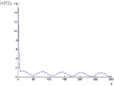
Figure 1: $|e(t)|_{2}$ vs $t$

VIII Asynchronous Operation

In this section we show that with minor modification, the algorithm we have been studying, namely (2), can be implemented asynchronously. The relevant update rules are given by (38). Since these rules are defined with respect to different and unsynchronized time sequences, for convergence analysis one needs to derive a model on which all update rules evolve synchronously with respect to a single time scale. Such a model is given by (39). Having accomplished this, we then establish the correctness of (38), but only for the case when there are no communication delays. The more realistic version of the problem in which delays are explicitly taken into account is treated in [10]. The ideas exploited there closely parallel those used to analyze the asynchronous version of the unconstrained consensus problem treated in [44].

Let $t$ now take values in the real time interval $[0.\infty)$. We begin by associating with each agent $i$, a strictly increasing, infinite sequence of event times $t_{i1},t_{i2},\ldots$ with the understanding that $t_{i1}$ is the time agent $i$ initializes its state and the remaining $t_{ik},\;k>1$ are the times at which agent $i$ updates its state. Between any two successive event times $t_{ik}$ and $t_{i(k+1)}$, $x_{i}(t)$ is held constant. We assume that for any $k\geq 1$, $x_{i}(t)$ equals its limit from above as $t$ approaches $t_{ik}$; thus $x_{i}(t)$ is constant on each open half interval $[t_{ik},t_{i(k+1)}),\;\;k\geq 1$.

We assume that for $i\in\{1,2,\ldots,m\}$, agent $i$’s event times satisfies

$$\bar{T}_{i}\geq t_{i(k+1)}-t_{ik}\geq T_{i},\;\;\;\;k\in\{1,2,\ldots\}$$ (37)

where $\bar{T}_{i}$ and $T_{i}$ are positive numbers such that $\bar{T}_{i}>T_{i}$. Thus the event times of agent $i$ are distinct and the difference between any two successive event times cannot be too large. We make no assumptions at all about the relationships between the event times of different agents. In particular, two agents may have completely different unsynchronized event time sequences.

We assume, somewhat unrealistically, that at each of its event times $t_{ik}$, agent $i$ is able to acquire the state $x_{j}(t_{ik})$ of each of its “neighbors” where by a neighbor of agent $i$ at time $t_{ik}$ is meant any agent in the network whose state is available to agent $i$ at time $t_{ik}$. In the more realistic version of the problem treated in [10], it is assumed that $x_{j}(t_{ik})$ is only available to agent $i$ after a delay which accounts both for transmission time and the fact that the time at which $x_{j}(t_{ik})$ is acquired is typically some time in between $t_{ik}$ and one of agent $i$’s subsequent event times. There are some subtle issues here in setting up an appropriate model; we refer the reader to [10] for an explanation of what they are and how they are addressed.

In the sequel, for $k>1$ we write ${\cal N}_{i}(t_{ik})$ for the set of labels of agent $i$’s neighbors at time $t_{ik}$ while $k=1$ we define ${\cal N}_{i}(t_{i1})=i$. Since agent $i$ is always taken to be a neighbor of itself, ${\cal N}_{i}(t_{ik})$ is never empty.

Prompted by (2), the update rule for agent $i$ we want to consider for the asynchronous case is

$$x_{i}(t_{i(k+1)})=x_{i}(t_{ik})-\frac{1}{m_{i}(t_{ik})}P_{i}\left(m_{i}(t_{ik})x_{i}(t_{ik})-\sum_{j\in{\cal N}_{i}(t_{ik})}x_{j}(t_{ik})\right)$$ (38)

where $k\geq 1$, and for $j\in{\cal N}_{i}(t_{ik})$, $m_{i}(t_{ik})$ is the number of labels in ${\cal N}_{i}(t_{ik})$, and as before, $P_{i}$ is the orthogonal projection on the kernel of $A_{i}$.

To proceed we need a common time scale on which all $m$ agent update rules can be defined. For this, let $t_{1}=\max_{i}\{t_{i1}\}$ and write ${\cal T}_{i}$ for the event times of agent $i$ which are greater than or equal to $t_{1}$. Let ${\cal T}$ denote the set of all event times of all $m$ agents which are greater than or equal to $t_{1}$. Thus ${\cal T}$ is the union of the ${\cal T}_{i}$. Relabel the times in ${\cal T}$ as $t_{1},t_{2},\ldots,t_{p},\ldots$ so that $t_{p}<t_{p+1}$ for $p\geq 1$. We define the extended neighbor set of agent $i$, written $\bar{{\cal N}}_{i}(p)$, to be ${\cal N}_{i}(t_{p})$ if $t_{p}$ is an event time of agent $i$. For times $t_{p}\in{\cal T}$ which are not event times of agent $i$, we define $\bar{{\cal N}}_{i}(p)=\{i\}$. Doing this enables us to extend the domain of applicability of update rule (38) from ${\cal T}_{i}$ to all of ${\cal T}$. In particular, for $p\geq 1$,

$$x_{i}(t_{p+1})=x_{i}(t_{p})-\frac{1}{\bar{m}_{i}(p)}P_{i}\left(\bar{m}_{i}(p)x_{i}(t_{p})-\sum_{j\in\bar{{\cal N}}_{i}(p)}x_{j}(t_{p})\right)$$ (39)

where $\bar{m}_{i}(p)$ is the number of indices in $\bar{{\cal N}}_{i}(p)$. The validity of this formula is a simple consequence of the assumption that for $i\in\{1,2,\ldots,m\}$, $x_{i}(t)$ is constant on each open half interval $[t_{ik},t_{i(k+1)}),\;\;k\geq 1$.

Observe that (39) is essentially the same as update rule (2) except that extended neighbor sets replace the original neighbor sets. As with the synchronous case, convergence depends on connectivity of the graphs determined by the neighbor sets upon which update rules (39) depend. Accordingly, for each $p\geq 1$ we define the extended neighbor graph $\bar{\mathbb{N}}(p)$ to be that directed graph in ${\cal G}_{sa}$ which has an arc from vertex $j$ to vertex $i$ if $j\in\bar{{\cal N}}_{i}(p)$. The following is an immediate consequence of Theorem 1.

Theorem 4

Suppose each agent $i$ updates its state $x_{i}(t)$ according to rule (38). Suppose in addition that for some positive integer $l$, the sequence of extended neighbor graphs $\bar{\mathbb{N}}_{i}(p),\;p\geq 1$ is repeatedly jointly strongly connected. Then there exists a positive constant $\lambda<1$ for which all $x_{i}(t_{p})$ converge to the same solution to $Ax=b$ as $p\rightarrow\infty$, as fast as $\lambda^{p}$ converges to $0$.

Perhaps of greatest interest is the situation when the original neighbor graph $\mathbb{N}(t)$ is independent of time. In this case it is possible to address convergence without reference to extended neighbor graphs.

Corollary 2

Suppose that the original neighbor graph $\mathbb{N}(t)$ is independent of time and strongly connected. Suppose each agent $i$ updates its state $x_{i}(t)$ according to rule (38). Then there exists a positive constant $\lambda<1$ for which all $x_{i}(t_{p})$ converge to the same solution to $Ax=b$ as $p\rightarrow\infty$, as fast as $\lambda^{p}$ converges to $0$.

The proof of Corollary 2 depends on the following lemma.

Lemma 6

Suppose that the original neighbor graph $\mathbb{N}(t)$ is a constant graph $\mathbb{N}$. For $i\in\mathbf{m}$, let $\bar{T}_{i}$ be an upper bound on the difference between each pair of successive event times of agent $i$. Then for any pair of event times $t_{a},t_{b}\in{\cal T}$ satisfying $t_{b}-t_{a}\geq\max\{\bar{T}_{1},\bar{T}_{2},\ldots,\bar{T}_{m}\}$, $\mathbb{N}$ is a spanning subgraph of the composed graph $\bar{\mathbb{N}}(b)\circ\bar{\mathbb{N}}(b-1)\cdots\circ\bar{\mathbb{N}}(a)$.

Proof of Lemma 6: Let ${\cal N}_{i}$ denote the neighbor set of agent $i$. For $i\in\mathbf{m}$, $t_{i(j+1)}-t_{ij}\leq\bar{T}_{i}\leq t_{b}-t_{a},\;j\geq 1$. Therefore the set $\{t_{a},t_{(a+1)},\ldots,t_{b}\}$ must contain at least one event time $t_{p_{i}}$ of each agent $i$. Since $\bar{{\cal N}}_{i}(p_{i})={\cal N}_{i},\;i\in\mathbf{m}$, for each $j\in{\cal N}_{i}$ there must be an arc from $j$ to $i$ in $\bar{\mathbb{N}}(p_{i})$. It follows from the definition of $\mathbb{N}$, that its arc set must be contained in the union of the arc sets of the graphs $\bar{\mathbb{N}}(a),\bar{\mathbb{N}}(a+1),\ldots,\bar{\mathbb{N}}(b)$. But the arc set of the union of a finite number of graphs in ${\cal G}_{sa}$ is always a subset of the arc set of their composition [35]. Therefore the lemma is true.  

Proof of Corollary 2: Set $T_{\max}=\max\{\bar{T}_{1},\bar{T}_{2},\ldots,\bar{T}_{m}\}$ and $T_{\min}=\min\{T_{1},T_{2},\ldots,T_{m}\}$ and let $q$ be any positive integer for which $T_{\max}\leq qT_{\min}$. Let $a$ and $b$ be positive integers satisfying $b-a=mq$. We claim that $t_{b}-t_{a}\geq T_{\max}$. To prove that this is so, suppose the contrary, namely that $t_{b}-t_{a}<T_{\max}$. Then $t_{b}-t_{a}<qT_{\min}$. But for each $i\in\mathbf{m}$, $T_{\min}$ is no larger than the time between any two successive event times of agent $i$. Thus the closed interval $[t_{a},t_{b}]$ must contain at most $q$ event times of agent $i$. Since there are $m$ agents, $[t_{a},t_{b}]$ must contain at most $mq$ event times. Therefore $b-a<mq$ which is a contradiction.

In view of the preceding, $t_{b}-t_{a}\geq T_{\max}$ for any positive integers $a$ and $b$ satisfying $b-a=mq$. Therefore, by Lemma 6, $\mathbb{N}$ must be a spanning subgraph of the composed graphs $\bar{\mathbb{N}}(b)\circ\bar{\mathbb{N}}(t_{b-1})\cdots\circ\bar{\mathbb{N}}(a)$ for all such $a$ and $b$. But $\mathbb{N}$ is strongly connected so each such composed graph must be strongly connected as well. Therefore the sequence of graphs $\bar{\mathbb{N}}(1),\bar{\mathbb{N}}(2),\ldots$ is repeatedly jointly strongly connected by successive subsequences of length $mq$. From this and Theorem 4 it follows that Corollary 2 is true.  

IX Least Squares

A limitation of the algorithm we have been discussing is that it is only applicable to linear equations for which there are solutions. In this section we explain how to modify the algorithm so that it can obtain least squares solutions to $Ax=b$ even in the case when $Ax=b$ does not have a solution. As before, we will approach the problem using standard consensus concepts rather than the more restrictive concepts based on distributed averaging. To keep things simple, we will assume that the $A_{i}$ are full column rank matrices.

By the least squares solution to $Ax=b$ is meant a value of $x$ for which $A^{\prime}Ax=A^{\prime}b$. As is well known, least squares solutions always exist, even if $Ax=b$ does not have a solution. It is very easy to verify that a common least squares solution $x$ to all of the agent equations $A_{j}x=b_{j},\;j\in\mathbf{m}$ will not exist unless $Ax=b$ has a solution. Thus if a decentralized least squares solution to $Ax=b$ is to be obtained in accordance with the agreement principle, then each agent must solve a different problem. To understand what that problem might be, consider for example the situation in which there are three agents. Suppose that the state $x_{i}$ of agent $i$ is augmented with two additional $n$-vectors, namely $y_{i}$ and $z_{i}$ and that agents $1$, $2$ and $3$ are tasked to solve the linear equations

$$A_{1}^{\prime}A_{1}x_{1}+y_{1} = A_{1}^{\prime}b_{1}$$

$$A_{2}^{\prime}A_{2}x_{2}+z_{2} = A_{2}^{\prime}b_{2}$$

$$A_{3}^{\prime}Ax_{3}-y_{3}-z_{3} = A_{3}^{\prime}b_{3}$$

respectively. As we will show, it is always possible for the agents to do this and the same time to obtain values of the $x_{i},y_{i}$ and $z_{i}$ for which the three augmented state vectors $\bar{x}_{i}=\left[\matrix{x_{i}^{\prime}&y_{i}^{\prime}&z_{i}^{\prime}}\right]^{\prime},\;i\in\mathbf{3}$ are the same.

The existence of a vector $\bar{x}=\left[\matrix{x^{\prime}&y^{\prime}&z^{\prime}}\right]^{\prime}$ for which $\bar{x}_{i}=\bar{x},\;i\in\mathbf{3},$ is equivalent to the existence to a solution to the equations $A_{1}^{\prime}A_{1}x+y=A_{1}^{\prime}b_{1}$, $A_{2}^{\prime}Ax+z=A_{2}^{\prime}b_{2}$, and $A_{3}^{\prime}A_{3}x-y-z=A_{3}^{\prime}b_{3}$. In matrix terms, existence amounts to asking whether or not the equation $M\bar{x}=q$ has a solution where

$$M=\left[\matrix{A_{1}^{\prime}A_{1}&I&0\cr A_{2}^{\prime}A_{2}&0&I\cr A_{3}^{\prime}A_{3}&-I&-I}\right]\;\;\;\;{\rm and}\;\;\;\;\;\;q=\left[\matrix{A_{1}^{\prime}b_{1}\cr A_{2}^{\prime}b_{2}\cr A_{3}^{\prime}b_{3}}\right].$$

Note that by simply adding block rows block rows $1$ and $2$ of $\left[\matrix{M&q}\right]$ to block row $3$, one obtains the matrix $\left[\matrix{\bar{M}&\bar{q}}\right]$ where

$$\bar{M}=\left[\matrix{A_{1}^{\prime}A_{1}&I&0\cr A_{2}^{\prime}A_{2}&0&I\cr A_{1}^{\prime}A_{1}+A_{2}^{\prime}A_{2}+A_{3}^{\prime}A_{3}&0&0}\right]$$

and

$$\bar{q}=\left[\matrix{A_{1}^{\prime}b_{1}\cr A_{2}^{\prime}b_{2}\cr A^{\prime}_{1}b_{1}+A^{\prime}_{2}b_{2}+A_{3}^{\prime}b_{3}}\right].$$

Clearly the set of solutions to $M\bar{x}=q$ is the same as the set of solutions to $\bar{M}\bar{x}=\bar{q}$ because the matrices $\left[\matrix{M&q}\right]$ and $\left[\matrix{\bar{M}&\bar{q}}\right]$ are row equivalent. It is obvious that $\bar{M}$ has linearly independent columns because $A_{1}^{\prime}A_{1}+A_{2}^{\prime}A_{2}+A_{3}^{\prime}A_{3}$ is nonsingular; therefore $\bar{M}$ is nonsingular. As a result, a solution to $M\bar{x}=q$ must exist. Note in addition, that since such a solution must also satisfy $\bar{M}\bar{x}=\bar{q}$, $x$ must satisfy $(A_{1}^{\prime}A_{1}+A_{2}^{\prime}A_{2}+A_{3}^{\prime}A_{3})x=A_{1}^{\prime}b_{1}+A_{2}^{\prime}b_{2}+A_{3}^{\prime}b_{3}$ which is the least squares equation $A^{\prime}Ax=A^{\prime}b$. Therefore $x$ solves the least squares problem.

Recall that the idea exploited earlier in the paper for crafting an algorithm for solving $Ax=b$, was that if each agent $i$ were able to compute a solution $x_{i}$ to its own equation $A_{i}x_{i}=b_{i}$ and at the same time all agents were able to reach a consensus in that all $x_{i}$ were equal, then automatically each $x_{i}$ would necessarily satisfy $Ax_{i}=b$. This led at once to the linear iterations (2) which provide distributed solutions to $Ax=b$. Since with obvious modification, the same idea applies to the least squares problem under consideration here, it is clear that the same approach will lead to linear iterations which provide a distributed solution to the least squares equation $A^{\prime}Ax=A^{\prime}b$. The update equations in this case are identical with those in (2) except that in place of and $x_{i}$ and $P_{i}$ one would use the $\bar{x}_{i}$ and $\bar{P}_{i}$ where $\bar{P}_{i}$ is the orthogonal projection matrix on the kernel of the $i$th block row in $M$. Under exactly the same the conditions as those stated in Theorem 1, the $x_{i}$ so obtained will all converge exponentially fast to the desired least squares solution.

IX-A Generalization

The idea just illustrated by example, generalizes in a straight forward way to any $m$ agent network. The first step would be to pick any $m$ vertex graph tree graph $\mathbb{T}$ and orient it. Agent $i$’s augmented state would then be of the form $\bar{x}_{i}=\left[\matrix{x_{i}^{\prime}&x_{i1}^{\prime}&x_{i2}^{\prime}&\ldots&x_{i(m-1)}^{\prime}}\right]^{\prime}$ where all $x_{ij}\in\mathbb{R}^{n}$. Instead of solving $A_{i}x_{i}=b_{i}$, agent $i$ would be tasked with solving $\left[\matrix{A_{i}^{\prime}A_{i}&h_{i}\otimes I}\right]\bar{x}_{i}=A_{i}^{\prime}b_{i}$ where $h_{i}$ is the $i$th row of the $m\times(m-1)$ incidence matrix of $\mathbb{T}$. At the same time, all $m$ agents would be expected to reach a consensus in which all $\bar{x}_{i}$ are equal. Were a consensus reached at a value $\bar{x}=\left[\matrix{x^{\prime}&y_{1}^{\prime}&y_{2}^{\prime}&\ldots&y_{m}^{\prime}}\right]^{\prime}$, then $\bar{x}$ would have to satisfy the equation $M\bar{x}=q$ where

$$M=\left[\matrix{A_{1}^{\prime}A_{1}&\cr\vdots&H\otimes I\cr A_{m}^{\prime}A_{m}&}\right]\;\;\;{\rm and}\;\;\;q=\left[\matrix{A_{1}^{\prime}b_{1}\cr\vdots\cr A_{m}^{\prime}b_{m}}\right].$$

We claim that a solution to $M\bar{x}=q$ must exist and that the sub-vector $x$ within $\bar{x}$ is the solution to the least squares problem. To understand why, first note that the block rows of $H\otimes I$ sum to zero because the rows of $H$ sum to zero. Thus if $E$ is product of elementary row matrices which adds the first $(m-1)$ block rows of $H\otimes I$ to the last, then $E(H\otimes I)$ must be of the form

$$E(H\otimes I)=\left[\matrix{D\cr 0}\right]_{nm\times(m-1)n}$$

where $D$ is a square matrix. Moreover $D$ must be nonsingular because the ${\rm rank\;}E(H\otimes I)={\rm rank\;}H\otimes I$ and ${\rm rank\;}H\otimes I=(m-1)n$. This last rank identity is a consequence of the fact that the rank of an incidence matrix of an $m$ vertex connected graph, namely ${\rm rank\;}H$, equals $m-1$.

Next observe that the set of solutions to $M\bar{x}=q$ is the same as the set of solutions to $EM\bar{x}=Eq$. But

$$EM=\left[\matrix{A_{1}^{\prime}A_{1}&\cr\vdots&D\cr A_{m-1}^{\prime}A_{m-1}&\cr A^{\prime}A&0}\right]\;\;\;{\rm and}\;\;\;Eq=\left[\matrix{A_{1}^{\prime}b_{1}\cr\vdots\cr A_{m-1}^{\prime}b_{m-1}\cr A^{\prime}b}\right].$$

Moreover $EM$ is obviously nonsingular so a solution to $EM\bar{x}=Eq$ and consequently $M\bar{x}=q$ exists. Note in addition, that since such a solution must also satisfy $EM\bar{x}=Eq$, $x$ must satisfy $A^{\prime}Ax=A^{\prime}b$. Therefore $x$ solves the least squares problem.

We have just shown that if each agent $i$ updates its augmented state $\bar{x}_{i}(t)$ along a path for which $\left[\matrix{A_{i}^{\prime}A_{i}&h_{i}\otimes I}\right]\bar{x}_{i}(t)=A_{i}^{\prime}b_{i}$, so that $\bar{x}_{i}(t)$ reaches a limit which agrees with the augmented states of all other agents, then the limiting value of the sub-vector $x_{i}(t)$ will solve the least squares problem. The agent update equations for accomplishing this are identical to those in (2) except that in place of and $x_{i}$ and $P_{i}$, agent $i$ would use the $\bar{x}_{i}$ and $\bar{P}_{i}$ where $\bar{P}_{i}$ is the orthogonal projection matrix on the kernel of $\left[\matrix{A_{i}^{\prime}A_{i}&h_{i}\otimes I}\right]$. Under exactly the same the conditions as stated in Theorem 1, the $x_{i}$ so obtained will all converge exponentially fast to the desired least squares solution.

Although the algorithm just described solves the distributed least squares problem, it has several shortcomings. First, there must be a network wide design step in which $\mathbb{T}$ is specified; this conceivably can be accomplished in a distributed manner. Second, the size of the augmented state vector of each agent is $nm$ which does not scale well with the number of agents in the network. It is possible to significantly improve on the scaling problem if neighbor relations are time invariant and there is bi-directional communication between neighbors. How to do this will be addressed in another paper.

X Concluding Remarks

In this paper we have described a distributed algorithm for solving a solvable linear equation and given necessary and sufficient conditions for it to generate a sequence of estimates which converge to a solution exponentially fast. For the case when the equation admits a unique solution, we have derived an expression for a worst case geometric convergence rate. We have shown that with minor modification, the algorithm can track the solution to $Ax=b$ if $A$ and $b$ change with time, provided the rates of change of these two matrices are sufficiently small. We have show that the same algorithm can function asynchronously provided there are no communications delays and we have sketched a new idea for obtaining least squares solutions to $Ax=b$ which can be used even if $Ax=b$ has no solution.

We have left a number of issues opened for future research. One is to figure out what the relationship is between the parameter $\rho$ which appears in the convergence rate bound $\rho$, and a conditioning number of $A$. Another is to more tightly quantify the relationship between the variations in $A$ and $b$ in the event they are time varying, and the tracking error $e$. Yet another is to modify the least squares algorithm discussed in §IX to reduce the amount of information which needs to be transmitted between agents. This last issue will be addressed in a future paper.

References

- [1] S. Mou, J. Liu, and A. S. Morse. An distributed algorithm for solving a linear algebraic equation. In Proceedings of the 51st Annual Allerton Conference on Communication, Control, and Computation, pages 267–274, 2013.
- [2] A. Margaris. Parallel implementation of the jacobi linear algebraic system solver. In Proceedings of the 3rd Balkan Conference in Informatics, 2007.
- [3] C. K. Koc, A. Guvenc, and B. Bakkaloglu. Exact solution of linear equations on distributed-memory processors. In Proc. 14th IMACS World Congress on Computational and Applied Mathematics, pages 1339–1341, 1994.
- [4] C. Andersson. Solving linear equations on parallel distributed menory architectures by extrapolation. Technical report, Royal Institute of Technology, 1997.
- [5] David M. Young. Iteratice Methods for Solving Partial Difference Equations of Elliptical Type. PhD thesis, Harvard University, 1950.
- [6] R. Gordon, R. Bender, and G. T. Herman. Algebraic reconstruction techniques {ART} for three-dimensional electron microscopy and x-ray photography. Journal of Theoretical Biology, pages 471 – 481, 1970.
- [7] L. Xiao, S. Boyd, and S. Lall. A scheme for robust distributed sensor fusion based on average consensus. In Proc. Fourth International Symposium on Information Processiing in Sensor Networks, pages 63–70.
- [8] S. Kar, J. M. F. Moura, and K. Ramanan. Distributed parameter estimation in sensor networks: Nonlinear observation models and imperfect communication. IEEE Transactions on Information Theory, pages 1 – 52, 2012.
- [9] U A Khan and J M F Moura. Distributed kalman filters in sensor networks: Bipartite fusion graphs. In Proc. Workshop on Statisitical Signal Processing, pages 700–704, 2007.
- [10] J. Liu, S. Mou, and A. S. Morse. An asynchronous distributed algorithm for solving a linear algebraic equation. In Proceedings of the 2013 IEEE Conference on Decision and Control, pages 5409–5414, 2013.
- [11] A. Nedic and A. Ozdaglar. Distributed sub-gradient methods for multi-agent optimization. IEEE Transactions on Automatic Control, pages 48–61, 2009.
- [12] K. I. Tsianos and M. G. Rabbat. Distributed strongly convex optimization. the 50th Annual Allerton Conference on Communication, Control, and Computing, pages 593–600, 2012.
- [13] D. Jakovetic, J. M. F. Moura, and J. Xavier. Distributed nesterov-like gradient algorithms. Proc. of the 51st IEEE Conference on Decesion and Control, pages 5459–5464, 2012.
- [14] D. Jakovetic, J. M. F. Moura, and J. Xavier. Fast distributed gradient methods. IEEE Transactions on Automatic Control, (5):1131–1146, 2014.
- [15] A. Nedic, A. Ozdaglar, and P. A. Parrilo. Constrained consensus and optimization in multi-agent networks. IEEE Transactions on Automatic Control, pages 922–938, 2010.
- [16] K. I. Tsianos, S. Lawlor, and M. G. Rabbat. Push-sum distributed averaging for convex optimization. the 51st IEEE Conference on Decision and Control, pages 5453–5458, 2012.
- [17] J. C. Duchi, A. Agarwal, and M. J. Wainwright. Dual averaging for distributed optimization: Convergence analysis and network scaling. IEEE Transactions on Automatic Control, (3):592–606, 2012.
- [18] T. Chang, A. Nedic, and A. Scaglione. Distributed constrained optimization by consensus-based primal-dual perturbation method. IEEE Transactions on Automatic Control, (6):1524–1538, 2014.
- [19] A. Nedic and A. Olshevsky. Distributed optimization over time-varying directed graphs. Proc. of the 52nd IEEE Conference on Decesion and Control, pages 6855–6860, 2013.
- [20] B. Gharesifard and J. Cortes. Continuous-time distributed convex optimization on directed graphs. IEEE Transactions on Automatic Control, 2013. to appear.
- [21] A. I. Chen and A. Ozdaglar. A fast distributed proximal-gradient method. the 50th Annual Allerton Conference on Communication, Control, and Computing, pages 601–608, 2012.
- [22] L. Xiao and S. Boyd. Fast linear iterations for distributed averaging. Systems and Control Letters, 53:65–78, 2004.
- [23] S. Boyd, A. Ghosh, B. Prabhakar, and D. Shah. Gossip algorithms: Design, analysis and applications. In Proceedings INFOCOM, 2005.
- [24] J. Liu, S. Mou, A. S. Morse, B. D. O. Anderson, and C. Yu. Deterministic gossiping. Proceedings of the IEEE, 99(9):1505–1524, 2011.
- [25] J. Liu and A. S. Morse. Asynchronous distributed averaging using double linear iterations. In Proceedings of the 2012 American Control Conference, pages 6620–6625, 2012.
- [26] D. Kempe, A. Dobra, and J. Gehrke. Gossip-based computation of aggregate information. In Proceedings of the 44th IEEE Symposium on Foundations of Computer Science, pages 482–491, 2003.
- [27] F. Benezit, V. Blondel, P. Thiran, J. N. Tsitsiklis, and M. Vetterli. Weighted gossip: Distributed averaging using non-doubly stochastic matrices. In Proceedings of the 2010 IEEE International Symposium on Information Theory, page 1753 1757, 2010.
- [28] A. Olshevsky and J. Tsitsiklis. Convergence speed in distributed consensus and averaging. SIAM J. Control and Optimization, pages 33–55, 2009.
- [29] A. D. Dominguez-Garcia and C. N. Hadjicostis. Distributed matrix scaling and application to average consensus in directed graphs. IEEE Transactions on Automatic Control, (3):667–681, 2014.
- [30] J. Lu and C. Y. Tang. Distributed asynchronous algorithms for solving positive definite linear equations over networks - part ii: wireless networks. In Proc first IFAC Workshop on Estimation and Control of Networked Systems, pages 258–264.
- [31] J. Lu and C. Y. Tang. Distributed asynchronous algorithms for solving positive definite linear equations over networks - part i: Agent networks. In Proc first IFAC Workshop on Estimation and Control of Networked Systems, pages 22–26.
- [32] R. Tron and R. Vidal. Distributed computer vision algorithms through distributed averaging. In IEEE Conference on Computer Vision and Pattern Recognition, pages 57–63, 2011.
- [33] P. Lin andW. Ren. Distributed constrained consensus in the presence of unbalanced switching graphs and communication delays. In Proc. of the 51st IEEE Conference on Decision and Control, pages 2238–2243, 2012.
- [34] S. Mou and A. S. Morse. A fixed-neighbor, distributed algorithm for solving a linear algebraic equation. In Proceedings of the 2013 European Control Confrence, pages 2269 – 2273, 2013.
- [35] M. Cao, A. S. Morse, and B. D. O. Anderson. Reaching a consensus in a dynamically changing environment – a graphical approach. SIAM J. on Control and Optimization, pages 575–600, February 2008.
- [36] A. Jadbabaie, J. Lin, and A. S. Morse. Coordination of groups of mobile autonomous agents using nearest neighbor rules. IEEE Transactions on Automatic Control, 46(6):988–1001, june 2003. also in Proc. 2002 IEEE CDC, pages 2953 - 2958.
- [37] V. D. Blondel, J. M. Hendrichkx, A. Olshevsky, and J. N. Tsitsiklis. Convergence in multiagent coordination, consensus, and flocking. In Proc. of the 44th IEEE Conference on Decision and control, pages 2996–3000, 2005.
- [38] E. Seneta. Non-negative Matrices and Markov Chains. Springer, 2006.
- [39] M. Cao, A. S. Morse, and B. D. O. Anderson. Reaching a consensus in a dynamically changing environment – convergence rates, measurement delays and asynchronous events. SIAM J. on Control and Optimization, pages 610–623, February 2008.
- [40] L. Moreau. Stability of multi-agent systems with time-dependent communication links. IEEE Transactions on Automatic Control, 50:169–182, 2005.
- [41] R. G. Gallager. Discrete Stochastic Processes. Kluwer Academic Publishers, 1996.
- [42] E. J. Candes, J. Romberg, and T. Tao. Robust uncertainty principles: Exact signal reconstruction from highly incomplete frequency information. IEEE Transactions on Information Theory, 52:489–509, 2006.
- [43] B. A. Francis and W. M. Wonham. The internal model principle of control theory. Automatics, pages 457–465, 1976.
- [44] M. Cao, A. S. Morse, and B. D. O. Anderson. Agreeing asynchronously. IEEE Transactions on Automatic Control, pages 1826–1838, 2008.