Testing Dissipative Magnetosphere Model Light Curves and Spectra with Fermi Pulsars

Abstract

We explore the emission properties of a dissipative pulsar magnetosphere model introduced by Kalapotharakos et al. (2014), comparing its high energy light curves and spectra, due to curvature radiation, with data collected by the Fermi LAT. The magnetosphere structure is assumed to be near the force-free solution. The accelerating electric field, inside the light-cylinder, is assumed to be negligible, while outside the light-cylinder it rescales with a finite conductivity ($\sigma$). In our approach we calculate the corresponding high energy emission by integrating the trajectories of test particles that originate from the stellar surface, taking into account both the accelerating electric field components and the radiation reaction forces. First we explore the parameter space assuming different value sets for the stellar magnetic field, stellar period, and conductivity. We show that the general properties of the model are in a good agreement with observed emission characteristics of young $\gamma$-ray pulsars, including features of the phase resolved spectra. Second we find model parameters that fit each pulsar belonging to a group of eight bright pulsars that have a published phase-resolved spectrum. The $\sigma$ values that best describe each of the pulsars in this group show an increase with the spin-down rate $(\dot{E})$ and a decrease with the pulsar age, expected if pair cascades are providing the magnetospheric conductivity. Finally, we explore the limits of our analysis and suggest future directions for improving such models.

1. Introduction

Pulsars are collapsed cores of massive stars spinning at periods in the range $\sim 10^{-3}-10$ sec. They are capable of radiating at almost all spectral wavelengths (from radio to $\gamma$-rays), although only a small subset have detected $\gamma$-ray pulsations. Their emission is highly anisotropic, originating from particles accelerated along the open magnetic field lines by intense electric fields induced by their magnetic field rotation. When pulsars display $\gamma$-ray emission, most of their luminosity is emitted in $\buildrel>\over{\sim}100$ MeV $\gamma-$rays. As such they have been one of the major class of objects studied by the Fermi $\gamma$-ray Space Telescope (Fermi), using the Large Area Telescope (LAT) (Atwood et al., 2009). The release of the $2^{nd}$ Fermi Pulsar catalog (2PC) (Abdo et al., 2013), presents light curves and spectra of 117 $\gamma$-ray pulsars. Of these, 41 are radio-loud $\gamma$-ray pulsars discovered through radio timing, 36 are new pulsars discovered through their $\gamma$-ray pulsations alone, and a surprising 40 are radio-loud millisecond pulsars. We note that for all the radio-loud Fermi pulsars the radio luminosity is orders of magnitude smaller than that of $\gamma$-rays. Nonetheless, since the number of radio photons far exceeds the number of the $\gamma$-ray photons radio detection is easier, while $\gamma$-ray detection is efficient for the nearer and more energetic objects (Abdo et al., 2013).

Pulsar radiation has been studied over the years with a variety of models employing different assumptions about the location and geometry of emission zones, such as the Polar Cap (PC) (Daugherty & Harding, 1996), the Outer Gap (OG) (Cheng et al., 1986), (Romani & Yadigaroglu, 1995), the Slot Gap (SG) (Arons, 1983), Muslimov & Harding (2004), Separatrix Layer (SL)(Bai & Spitkovsky, 2010) and current sheet (Uzdensky & Spitkovsky, 2014; Pétri, 2012a; Contopoulos & Kalapotharakos, 2010; Kalapotharakos et al., 2012b, 2014). Many models, such as SG and OG implement curvature radiation (as in this paper) to describe the GeV radiation, while others implement synchrotron radiation powered by the reconnection in the current sheet (Lyubarskii, 1996; Uzdensky & Spitkovsky, 2014). The increased sensitivity of the Fermi LAT, with its first observations of a simple exponential cutoff of the Vela pulsar spectrum (Abdo et al., 2009), ruled out the PC emission model which predicted a super-exponential cutoff, due to magnetic pair attenuation near the neutron star surface. This result, later confirmed for a number of other pulsars, established that the pulsar $\gamma$-ray emission originates in the outer magnetosphere, with the OG and the SG models better fitting observations. However, none of these outer magnetosphere emission models can currently account for the entire pulsar light curve phenomenology (for example see Romani & Watters, 2010; Pierbattista et al., 2012, 2014). Furthermore, none of these models are consistent with global magnetosphere properties, such as current closure.

The recent development of 3D, global, force-free electrodynamics (FFE) (Spitkovsky, 2006; Kalapotharakos & Contopoulos, 2009; Pétri, 2012b), Magnetohydrodynamical (Komissarov, 2006; Tchekhovskoy et al., 2013) and Particle in Cell (Philippov & Spitkovsky, 2014; Cerutti et al., 2014; Chen & Beloborodov, 2014) pulsar magnetosphere models gave an impetus to the study of pulsar magnetospheres by providing a more realistic picture of their outer field geometry than the vacuum model previously assumed. However, because the ideal MHD FFE regime precludes the existence of electric fields parallel to the magnetic field (${\bf E_{\parallel}}=0$) and thus the acceleration of particles and the emission of radiation, more realistic dissipative MHD magnetosphere models have been developed (Kalapotharakos et al., 2012c; Li et al., 2012). These models allow for ${\bf E_{\parallel}}\neq 0$ and therefore can accommodate the production of radiation. They are constructed by numerically evolving the time dependent Maxwell’s equations, while at the same time employing a form of Ohm’s law to relate the current density ${\bf J}$ to the fields. This has the general form

$$\mathbf{J}=c\rho\dfrac{\mathbf{E}\times\mathbf{B}}{E_{0}^{2}+B^{2}}+\sigma\mathbf{E_{\parallel}},$$ (1)

where $\mathbf{J}$ is the current density, $\mathbf{E}$ and $\mathbf{B}$ are the electric and magnetic field, and $E_{0}$ is defined by $B_{0}^{2}-E_{0}^{2}=\mathbf{B^{2}}-\mathbf{E^{2}}$ , $E_{0}B_{0}=\mathbf{E\cdot B}$, $E_{0}\geq 0$. $E_{0}$ is a term that prevents the drift velocity and hence the current from becoming superluminal, while $\sigma$ is a phenomenological conductivity, used to relate ${\bf E_{\parallel}}$ to the current density ${\bf J}$, measured in units of the pulsar rotation frequency $\Omega$, the fundamental frequency in the problem. The macroscopic spatial $\sigma$ distribution should be consistent with the underlying microphysics. However, the dependence of the conductivity on the microphysics is still not understood. Thus, the goal of the recent study of global dissipative MHD magnetosphere models is to explore the main properties of various $\sigma$ values and distributions. In our first studies (Kalapotharakos et al., 2012a, c) a conductivity that is mainly uniform (in space) and constant in time was assumed. In Kalapotharakos et al. (2014), we have started to implement a broad range of conductivity values along the open magnetic field lines while the FFE (in reality highly conductive) condition was applied in the ‘closed’ region.

We have employed these dissipative magnetosphere models to generate model $\gamma$-ray light-curves (Kalapotharakos et al., 2012c, 2014) due to curvature radiation (CR). To this end, we calculate the trajectories and Lorentz factors $\gamma_{L}$ of radiating particles, under the influence of both the accelerating magnetospheric electric fields and CR-reaction. This approach allowed us to relate the observed pulsar emission properties to those of the model magnetospheres. Such observables are the separation (in phase) of the $\gamma-$ray light curve peaks $\Delta$ and also the lag $\delta$ between the radio emission and the first peak of the $\gamma-$ray light curve. It was found (Kalapotharakos et al., 2014) that matching the model $\delta-\Delta$ distribution with that obtained in the 2PC (Abdo et al., 2013) cannot be achieved with a $\sigma$ constant across the entire magnetosphere but requires essentially FFE (infinite conductivity, ${\bf E_{\parallel}}=0$) conditions interior to the light cylinder (LC), with radius $R_{\rm LC}=c/\Omega$, and large ($\sigma\buildrel>\over{\sim}30\Omega$) but finite conductivity outside the LC giving these models the nomenclature FIDO (FFE Inside, Dissipative Outside).

In the current paper we expand our study by considering the FIDO models that were presented in (Kalapotharakos et al., 2014) by exploring their energetic and spectral properties under certain simple assumptions. We attempt to compare the detailed luminosities and spectra of the dissipative magnetosphere models to those obtained by observations. To this end, rather than perform a statistical comparison of the FIDO model with the entire Fermi population, we decided to compare the phase-averaged and phase-resolved spectra predicted by the FIDO model with a few very luminous pulsars that have published phase-resolved spectra. This being the first comparison of spectra predicted by dissipative models with data, we chose to focus on individual pulsars by which we can better understand the model comparison. This comparison will provide the trends and will reveal the limitations of this model and its assumptions in describing the entire high energy pulsar phenomenology depicted by Fermi.

In §2 we describe the methods employed in our modeling of the pulsar magnetospheres and the production of the phase resolved spectra and in §3 we present our results. We conclude in §4 with a discussion of their importance of the results and directions to be followed in the future studies.

2. Methods

Figure 1.— Examples of photon light curves, between 100 MeV and 50 GeV, produced by a FIDO magnetosphere with $P=0.1s$, $B=4\cdot 10^{12}G$ and $\sigma=30\Omega$. From left to right are different $\zeta$ ($30^{\circ}$, $45^{\circ}$, $60^{\circ}$, $75^{\circ}$, $90^{\circ}$) while from top to the bottom are different $\alpha$ ($15^{\circ}$, $30^{\circ}$, $45^{\circ}$, $60^{\circ}$, $75^{\circ}$, $90^{\circ}$). The overlapping green dots are the phase resolved $E_{cut}$. The y axes are rescaled to the relative maximum of the light curve, the x axis is rotation phase, from 0 to 1. The values on the y axis are the values of the phase resolved $E_{cut}$ in GeV.

2.1. The Magnetosphere Structure

The magnetosphere structure is obtained by numerically solving the time dependent Maxwell equations

$$\dfrac{\partial\mathbf{B}}{\partial t}=-c\nabla\times\mathbf{E}$$ (2)

$$\dfrac{\partial\mathbf{E}}{\partial t}=c\nabla\times\mathbf{B}-4\pi\mathbf{J}$$ (3)

with a 3D finite difference time domain technique (Kalapotharakos & Contopoulos, 2009). We consider the presence of a dipole magnetic moment $\boldsymbol{\mu}$ at the center of the star and that the star itself is a perfect conductor; then the boundary condition on the stellar surface for the electric field is the FFE condition for a corotating magnetosphere:

$$\mathbf{E}+\mathbf{(\boldsymbol{\Omega}\times\mathbf{R})\times B}=0$$ (4)

The closure of the system requires a prescription for the current density J in terms of the fields (Eq. 1), as in Kalapotharakos et al. (2014). When $\sigma$ is very close to the FFE case ($\sigma\rightarrow\infty,E_{\parallel}\rightarrow 0,\dfrac{\partial\mathbf{E}}{\sigma\partial t}\rightarrow 0$), taking the parallel component of Eq. 3 it is possible to approximate the electric field parallel to the magnetic field as Kalapotharakos et al. (2014)

$$E_{\parallel}=\dfrac{c|(\nabla\times\mathbf{B})_{\parallel}|_{(\rm FFE)}}{4\pi\sigma}$$ (5)

where the FFE indication implies the corresponding FFE value.

As in Kalapotharakos et al. (2014), we start with a FFE global magnetosphere model implementing the FFE current density $J$ prescription (Gruzinov, 1999)

$$\mathbf{J}=c\rho\frac{\mathbf{E}\times\mathbf{B}}{B^{2}}+\frac{c}{4\pi}\frac{\mathbf{B\cdot\nabla\times B-E\cdot\nabla\times E}}{B^{2}}\mathbf{B}$$ (6)

and then compute $E_{\parallel}$ only outside the LC, located at radius $R_{\rm LC}=c/\Omega$, using the approximation in Eq. 5 of the prescription of Eq. 1 for $\sigma=0.3,1,3,5,10,30,60\Omega$ ($\sigma=30\Omega$ was used for the original FIDO model). We did not test higher $\sigma$ values since for these the corresponding cutoff energies $(E_{\rm cut})$ and total $\gamma$-ray luminosities ($L_{\gamma}$) are well below the ones observed by Fermi. In our FFE simulations we use a stellar radius $r_{\star}=0.2R_{\rm LC}$. Our computational domains extend up to $5R_{\rm LC}$ and the spatial resolution (i.e. the grid cell size) is $0.01R_{\rm LC}$. Each simulation has been evolved for  2 stellar rotations.

Here we would like to note that ideal (of infinite resolution) FFE simulations would lead to infinitesimally thin current sheets and hence to infinitely large $\nabla\times\mathbf{B}_{{\parallel}_{(\rm FFE)}}$ and $E_{\parallel}$ values lying within infinitesimally small volumes. However, in dissipative solutions (finite $\sigma$) the thickness of the current sheet is expected to be of the order of $c/\sigma$. In our FFE simulations the resolution is finite ($0.01R_{LC}$) and the corresponding current sheet is resolved within a few grid cells. This behavior mimics the finite thickness of the current sheet in dissipative solutions. This “artificial” FFE thickness of the current sheet is similar to that corresponding to “real” dissipative solutions with $\sigma=30\Omega$. Our base FIDO solution is the one with $\sigma=30\Omega$ presented in Kalapotharakos et al. 2014. We have checked that the results corresponding to FFE solutions with a spatial distribution of $E_{\parallel}$ based on Eq. 5 (assuming $\sigma=30\Omega$) and those of “true” dissipative solutions (using explicitly prescription 1) with uniform $\sigma=30\Omega$ provide very similar results.

We also checked the validity of this approximation by simulating a few FIDO magnetospheres for $\sigma=0.3,5\Omega$ and $10\Omega$ and various magnetic moment inclination angles with respect to the rotational axis, $\alpha$ (fixing the period, P, and B); we found that especially for $\alpha<45^{\circ}$ and for $\sigma\leq 5\Omega$ the field structure deviates substantially from the FFE field structure on which our approximation is based. This is primarily because $\sigma$ has been assumed to be uniform outside the light cylinder. However, the important region for the particle acceleration in the FIDO model is near the equatorial current sheet outside the light cylinder (Kalapotharakos et al. 2014). In the case of small $\sigma$ values, a more accurate treatment is needed (e.g. application of the smaller $\sigma$ values only near the equatorial current sheet). This study is beyond the scope of the current paper and will be addressed in a future work (see §4). In the rest of the paper we consider the FFE numerical models employing an $E_{\parallel}$ that rescales according to Eq. (5). This treatment, though simplistic, allows the exploration of the main trends and correlations among the various parameters taking into account a broad range of properties of the observed phenomenology (e.g. light curves, spectra).

2.2. Simulation of the emission

To simulate the $\gamma$-ray emission of the model pulsar magnetospheres we neglect the inverse Compton (IC) and synchrotron radiation (SR) contribution and consider only curvature radiation CR, (Jackson, 2001). In some models, where particles are energized by reconnection in current sheet (Uzdensky & Spitkovsky, 2014), SR is produced by high temperature particles up to 100 GeV. In the type of model we are considering here, where particles are energized only by the induced electric field parallel to the magnetic field, the particles can emit SR only if they acquire some pitch angles. In such “gap” models (Harding et al., 2008; Tang et al., 2008) SR does not give photons more energetic than 100 MeV. IC requires a high-altitude non-thermal X-ray emission component that is present only for a few Fermi pulsars such as the Crab. To save computational time in calculating the emission, a random subset of $1.5\cdot 10^{6}$ initial particle orbit positions were selected on the pulsar polar cap. Their orbits were integrated under the influence of the local parallel electric field $E_{\parallel}$ and losses due to curvature radiation to compute their Lorentz factor $\gamma_{L}$ as a function of position, in the non-rotating inertial frame. Then we selected randomly $5\cdot 10^{10}$ particles positions along these trajectories between the star surface and 2.5 times the light cylinder radius $R_{LC}$, where we computed the spectrum of the locally emitted CR and its direction $(\zeta,\phi)$, taking into account the time delays and assuming that the CR photons are emitted in the direction of particle motion ($\zeta$ is the observer’s inclination relative to the pulsar rotation axis and $\phi$ the azimuth). For each particle we calculated the number of photons emitted per second by CR and stored them in a 3D matrix: 100 bins of resolution for the azimuth $\phi$ (between $0^{\circ}$ and $360^{\circ}$), 180 bins of resolution for $\zeta$ (between $0^{\circ}$ and $180^{\circ}$) and 114 energy bins equally spaced logarithmically between 0.01 and 50 GeV.

We calculated the luminosity by rescaling the area of the polar cap according to the period of the star and to a fixed radius of 10 km (in the simulation of the FIDO model the radius was at 0.2$R_{LC}$) and the flux of particles from the surface with the Goldreich-Julian (GJ) density $\rho_{\rm GJ}$ (Goldreich & Julian (1969)), assuming the polar cap is small enough to consider the GJ charge density constant. The adopted $\rho_{\rm GJ}$ flux assumes that the multiplicity of the accelerated particles in the regions with high $E_{\parallel}$ is small ($\sim 1$). This assumption is reasonable given that much higher multiplicity leads to screening of the $E_{\parallel}$ over distances short enough to prevent fluxes $\gg\rho_{\rm GJ}$ of accelerated particles. This 3D grid allows us to calculate sky maps, light curves and phased resolved spectra. The sky maps are produced by summing up over the photon energy and plotting the resulting intensity in photons/s in ($\zeta,\phi$) coordinates. Summing over energy for a particular viewing angle $\zeta$ of the sky map produces a light curve. Phase-averaged spectra can be obtained by averaging the photon distribution in energy over $\phi$ for a chosen $\zeta$. Finally, phase-resolved spectra are obtained by collecting the spectra in each ($\zeta,\phi)-$bin. We applied this procedure to pulsar magnetospheres with a number of inclination angles $\alpha$ between the rotation and magnetic axes ($\alpha=15^{\circ},30^{\circ},45^{\circ},60^{\circ},75^{\circ},90^{\circ}$), different rotation periods ($0.01s,0.03s,0.1s,0.3s,1s$) and different magnetic fields at the stellar surface ($5\cdot 10^{11}$G, $10^{12}$G, $2\cdot 10^{12}$G, $4\cdot 10^{12}$G, $8\cdot 10^{12}$G, $3\cdot 10^{13}$G) assuming each time all the different conductivity values $(\sigma=0.3\Omega,1\Omega,3\Omega,5\Omega,10\Omega,30\Omega,60\Omega)$ mentioned in the previous section. Thus, we tested $(6\times 7\times 5\times 6=1260)$ different magnetosphere configurations.

The sky maps and light curves shown in Kalapotharakos et al. (2014) were computed for the bolometric luminosity, while here we computed sky maps and light curves in photons/s in the energy band $0.1-50$ GeV in order to compare with observed Fermi light curves and spectra. Our light curves in Figure 1 show some extra secondary peaks that do not appear in the bolometric light curves, due to relative spectral differences with phase. We generated sky maps and light curves in bolometric luminosity and they are very similar to those of Kalapotharakos et al. (2014) except for small differences in the relative heights of the light curve peaks (the maximum difference is $\lower 2.0pt\hbox{$\,\buildrel\scriptstyle<\over{\scriptstyle\sim}\,$}20\%$). This kind of difference is due to differences in sampling and/or binning. In addition, we smoothed the profiles (with a gaussian smoothing with $\Theta=3.6^{\circ}$) to reduce the numerical noise.

2.3. Comparison with the Fermi pulsars

We used the data from the 2PC, gathered with three years of observations acquired by the LAT on the Fermi satellite, except for the phase-resolved spectra that have appeared in different papers (DeCesar (2013), Abdo et al. (2010a), Abdo et al. (2010b)). These different works use data collected over different amounts of time (generally less than the 3 years of data used for 2PC) but they all analyze photons in the same energy range (between 100 MeV and 50 GeV like in the 2PC).

We study some particularly luminous $\gamma$-ray pulsars, in particular the ones that have a published phase resolved spectrum. This set of eight pulsars contains: J0007+7303 (CTA1 pulsar), J0534+2200 (Crab pulsar), J0633+1746 (Geminga pulsar), J0835-4510 (Vela pulsar), J1057-5226, J1709-4429, J1836+5925, J1952+3252. We identified a candidate light curve and its associated phase-resolved spectrum produced by our model for a combination of $\alpha$, $\zeta$, $\sigma$ that best describe those of each pulsar. We made a first selection using the number of peaks in the light curve. The sample of model light curves were generated at different viewing angles $\zeta$ (equivalent of the latitude) between $5^{\circ}$ and $90^{\circ}$ with a step of $5^{\circ}$. These 18 light curves were generated for each inclination angle and for $\sigma=1\Omega,5\Omega,30\Omega$. This grid was fine enough to resolve the single/double peaked attribute of the light curves, identifying the best values of $(\alpha,\zeta)$. We then used simulated magnetosphere models for the whole range of $\sigma$ noted above, selecting the closest P and B values to those of the real pulsars. For each combination of $\alpha$ and $\zeta$ selected we matched the cutoff energy $E_{cut}$ from the phase averaged spectra (an example in Figure 2) using the same form as was used to fit the pulsar spectra of the 2PC (Abdo et al., 2013)

$$\frac{dN}{dE}=K\left(\frac{E}{E_{0}}\right)^{-\Gamma}\exp\left(-\frac{E}{E_{cut}}\right)$$ (7)

Figure 2.— An example of a phase-averaged spectrum produced by the model (blue) and fitted to a power law with exponential cutoff (green). The red vertical line is the fit value of $E_{cut}$. The x axis is photon energy in eV, the y axis is a quantity proportional to the amplitude.

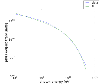
We looked for a candidate (considering the whole range of $\sigma$ values) with an $E_{cut}$ that was within a factor of 2 of that observed. We then matched the separation between the gamma-ray peaks (with a tolerance of 0.08 in phase, where 1.0 is the period), the evolution of light curves with energy predicted by the model, and the flux, in comparison with that observed in the 2PC. The distances used are those reported in the 2PC. Considering the maximum error in the distance measures and the maximum variation in the flux of the simulated light curves with respect to $\alpha$, and the assumed multiplicity of 1 in the particle flux, we accept a flux within a factor of 10 of the observed value. These were the primary features we considered in selecting candidate light curves and spectra. The other features we considered were the “half-power width” of the light curve peaks and the trend of the phase-resolved $E_{cut}$. We did not give as much importance to the spectral index $\Gamma$ because it is more strongly influenced by possible contributions from SR and IC emission. We note that the discrepancies in the model flux that we would have obtained considering the observed spectral index ($\Gamma$) value in the phase averaged spectrum were always less than 15%.

3. Results

3.1. General properties of the model

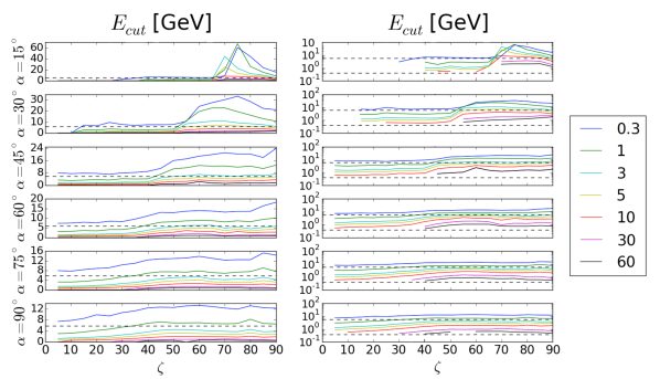
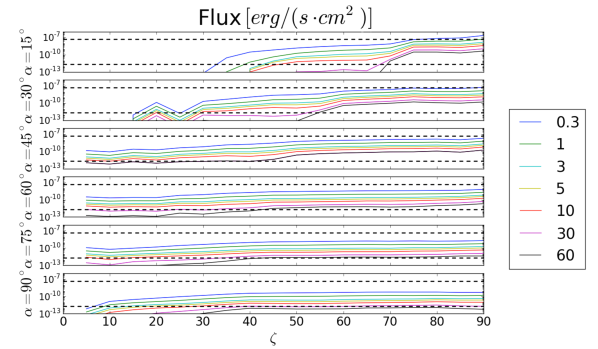
As was reported in Kalapotharakos et al. (2014) the FIDO model has the interesting property of reproducing the correlation between $\delta$ and $\Delta$ presented in the 2PC (Abdo et al., 2013). The simulated light curves in Figure 1 look similar to the observed light curves, except for some additional smaller peaks. In Figure 5 of the Appendix we show the luminosity skymaps of a FIDO magnetosphere with $P=0.1s$, $B=4\cdot 10^{12}G$ and $\sigma=5\Omega$; we also plotted the trends in flux and $E_{cut}$ with $\alpha$, $\zeta$ and $\sigma$. We notice that the flux and the $E_{cut}$ generally increase with $\zeta$ and decrease with $\sigma$, for fixed $\alpha$. They also increase with decreasing P and increasing B. The physical cause of these trends are that increasing $\zeta$ more closely approaches the more energetic main caustic (as we can see in the Appendix in Figure 5). Increasing $\sigma$ decreases the value of $E_{\parallel}$, the maximum value of the particle Lorentz factor $\gamma_{L}$ (as we noted in subsection 2.1) and hence the value of $E_{cut}$. Increasing B also increases $E_{\parallel}$ (fixing $\sigma$), while decreasing P reduces the LC radius and thus on the one hand decreases the radius of curvature of the particle trajectories (in absolute units) and on the other hand increases the absolute $E_{\parallel}$ values (the closer to the star the emitting region is the higher the corresponding field values are). These effects, in general, increase the $\gamma_{L}$ values, the corresponding photon energies ($E_{cut}$), and the total power emitted. Increasing $\alpha$ results in a decrease of $E_{cut}$ and of the flux: this is due to both $E_{\parallel}$ being smaller and the GJ charge density (Goldreich & Julian (1969)) at the surface of the polar-cap decreasing with $\alpha$, reaching 0 at $\alpha=90^{\circ}$.

In Figure 6, of the Appendix we show the dependence of the luminosity of our models with the pulsar period and magnetic field (red dots) as well as the observations of 2PC (blue dots). In Figure 7 we show the dependence of $E_{cut}$ for a pulsar with $P=0.1$ sec and $B=2\times 10^{12}$ G as a function of $\alpha,\zeta,\sigma$ while in Fig. 8 the dependence of flux of the same pulsar on the same parameters assuming a distance of 1 kpc. Generally, the model $E_{cut}$ values for $\sigma\geq 3\Omega$ match the observed values. while for $\sigma<3\Omega$ the model $E_{cut}$ values are larger than observed. The model flux values for all $\sigma$ are within the observed range, except for the largest $\sigma$ values at the smallest $\alpha$ and $\zeta$. Although the model fluxes are about a factor of ten below the highest observed fluxes at the largest $\alpha$, even for the lowest $\sigma$ values, Fig. 8 is only plotted for one value of $P$ and $B$ and does not show model fluxes for the full range of these values in the observed population.

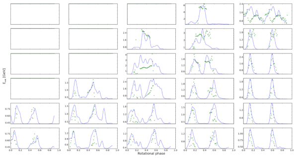
Another feature we investigate is the general trend of the phase resolved spectra. From the phase resolved spectra that are available it seems that the $E_{cut}$ is always higher in the $2^{nd}$ light curve peak or in the right part of a broad single peaked light curves. This behavior is followed by $\sim 55\%$ of our model light curves, $23\%$ do not show a significant difference in $E_{cut}$ between the two peaks, while $22\%$ exhibit the opposite behavior. So, according to the FIDO model, obtaining phase-resolved spectra from more pulsars should show some that do not follow the trend of higher $E_{cut}$ in the second peak.

In a few of the magnetosphere models, the luminosity exceeds $\dot{E}$. Since this cannot happen physically, the problem is linked to the following cause. The approximation of Eq. 5 forces the $E_{\parallel}$ to change linearly with respect to $\sigma$. Nonetheless, we found through full simulations using low $\sigma$ that this process is not exactly linear and the $E_{\parallel}$ saturates for low $\sigma$ values. Thus, whenever the $E_{\parallel}$ is higher than it should have been this can contribute to an overestimation of the luminosity. Finally, this effect is probably due to the overestimation of the distances of the given pulsars.

3.2. Model $\gamma$-ray pulsar identification

First we performed a blind-search to find the parameters giving light curves and spectra that best match those of the Fermi pulsars, disregarding any constraints from other wavelengths. We note that on the one hand the light-curve form is the most important feature for the determination of each pulsar’s $\alpha$ value and the Earth’s $\zeta$ value. On the other hand the $E_{\rm cut}$ and $L_{\gamma}$ values determine the corresponding $\sigma$ value. We found from one to three candidates per pulsar. But of the 8 pulsars for which we found model candidates with this blind-search, two did not have a good match with other wavelength constraints (taken from Pierbattista et al. (2014)). Looking for candidates again in the zone indicated by these constraints we found one possible candidate per pulsar, with a less-than-perfect light curve match but still reasonable. This fact shows that our model is not always able to identify in an unambiguous way a candidate that satisfies all our criteria simultaneously. We report the geometry and conductivity information of our candidates in Table 1 while the fluxes and the $E_{cut}$ are shown in Table 8.

Table 1FIDO Pulsar Candidates - Geometry.

Name	$\alpha$[∘]	$\zeta$6[∘]	$\alpha$[∘]	$\zeta$[∘]	$\sigma[\Omega]$	Radio
J0007+7303	–	–	30	73	10	quiet
J0534+2200	–	61	75	63	30	caustic
J0633+1746	–	$>60$	45	87	3	quiet
J0835-4510	70	64	60	50	10	loud
J1057-5226	–	–	45	61	30	loud
J1709-4429	–	53	45	55	10	loud
J1836+5925	–	–	90	40	1	quiet
J1952+3252	–	–	75	85	10	loud

Table 2FIDO Pulsar Candidates - Energetics

Name	$E_{cut}^{obs}$	$\Gamma^{obs}$	$F_{\gamma}^{obs}$	$E_{cut}$	$\Gamma$	$F_{\gamma}$	$\sigma[\Omega]$
J0007+7303	4.7	1.4	4.0	5.0	0.9	0.8	10
J0534+2200	4.2	1.9	13	3.4	1.3	16	30
J0633+1746	2.2	1.2	42	3.4	1.2	1.5	3
J0835-4510	3.0	1.5	91	4.1	1.4	19	10
J1057-5226	1.4	1.0	3.0	1.3	2.0	1.5	30
J1709-4429	4.2	1.6	14	4.2	1.1	1.1	10
J1836+5925	2.0	1.2	6.0	3.0	1.1	0.2	1
J1952+3252	2.5	1.5	1.4	2.2	1.4	0.7	10

We find a correlation between the $\sigma$ of the candidates and their $\dot{E}$ and the age estimate obtained through the period and period derivative (excluding the candidate for J1057-5226, since it seems to be an outlier). We fit these two correlations with a power law, using the large intervals we had on the $\sigma$ grid as errors:

$$y=a+b\cdot x^{c}$$ (8)

We obtained for the relation $\sigma-$ age:

$$a=-1\pm 3,b=32\pm 23,c=-0.36\pm 0.01$$ (9)

While for the relation $\sigma-\dot{E}$:

$$a=-6\pm 30,b=(7.80\pm 0.02)\times 10^{-5},$$ (10)

$$c=0.146\pm 0.004$$

both with $\chi^{2}_{red}\simeq 0.2$, where $\chi^{2}_{red}$ is the reduced $\chi^{2}$, that highlight the large error bar assumed. These relations are shown in Figures 3, 4.

Figure 3.— The conductivity, $\sigma$, for the best candidates as a function of pulsar characteristic age. The pulsars used in the fit are in blue; the one in red is J1057-5226 and was excluded from the fit; the solid black line is the power law found by the fit routine (see Eq. 9) .

Figure 4.— The conductivity, $\sigma$, for the best candidates as a function of pulsar spin down luminosity $\dot{E}$. The pulsars used in the fit are in blue; the one in red is J1057-5226 and was excluded from the fit; the solid black line is the power law found by the fit routine (see Eq. 10).

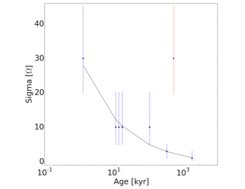
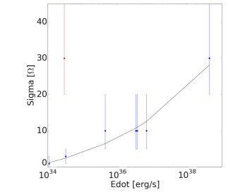
These two correlations are expected if higher $\sigma$ results from more efficient screening of $E_{\parallel}$ by pairs that are produced in greater numbers by younger, more energetic pulsars (Daugherty & Harding, 1982; Harding & Muslimov, 2011). Our 8 candidates do not reproduce all of the observed characteristics of these pulsars: two had a bit smaller flux than observed (within a factor of 15, J1709-4429, and 40, J0633+1746, instead of 10), two of them do not reproduce the observed bridge emission in the light curve (J0633+1746) or the off-peak emission present in the observed light curve (J1836+5925). For the candidate of radio quiet pulsar Geminga (J0633+1746) having a 0.5 peak separation, we interchanged the model peaks in order to match the observed relative peak heights, which we are free to do since our model light curve has no bridge emission. The J0007+7303 candidate has a smaller peak width than observed (the tolerance is $\pm 0.06$) and two candidates have phase resolved spectra that do not show the observed trends (J0007+7303, J1836+5925). In the Appendix, we show observed and model light curves and phase-resolved spectra for three of the pulsars, Vela, Crab and J1952+3252.

4. Conclusion

We have computed light curves, luminosities, phase-resolved and phase-averaged spectra for a large number of FIDO models (which were shown to reproduce the $\delta-\Delta$ distribution of 2PC) for different values of $\alpha,P$, $B$, $\sigma$ and $\zeta$. All of these emission characteristics of the model were compared with light curves, phase-averaged and phase-resolved spectra of eight bright pulsars studied with Fermi. In particular we explored whether the common trends found in the eight published phase-resolved spectra, such as a higher $E_{cut}$ in the second peak, are absolute predictions of the FIDO model. We found that this is in fact a common trend, but not absolute since the reverse trend (higher $E_{cut}$ in the first peak) or similar $E_{cut}$ in both peaks, is also predicted for a subset of parameters. It would therefore be of interest to produce phase-resolved spectra for a larger number of pulsars.

This work shows that the FIDO dissipative model merits further exploration, particularly with respect to the correlations seen in Figures 3 and 4. If these correlations are confirmed, it would strengthen the expected connection between screening of $E_{\parallel}$ by efficient pair production and high conductivity.

The major limitations of the present model are the assumption of FFE scaling of $E_{\parallel}$ with conductivity outside the light cylinder, and the assumption that the magnetosphere inside the light cylinder is completely FFE. The choice of spatial variation of the conductivity (infinite inside and finite outside the LC) was imposed by the need to reproduce the pulsar $\delta$-$\Delta$ (radio lag - peak separation) correlations. Consistency of the models with these correlations requires no (or very little) emission from within the LC, hence the FFE approximation for this region. Clearly, emission of radiation requires finite conductivity and non-zero $E_{\parallel}$ somewhere in the magnetosphere, necessarily outside the LC. A more realistic distribution of $\sigma$ likely requires its variation with distance along the field lines and from one line to another. This variation prescription should be eventually consistent with the related microphysical mechanisms (the details of which are not well understood, at present at least). Nonetheless, the overall distribution cannot be much different than that proposed in Kalapotharakos 2014, else it would be inconsistent with the $\gamma$-ray light curve correlations.

We have also explored the validity of the FIDO model by making some test simulations with low $\sigma$ outside the light cylinder, still assuming FFE conditions inside. It was found that the $E_{\parallel}$ in these simulations does not drop linearly with $\sigma$ for $\sigma<5\Omega$ and $\alpha<45^{\circ}$, primarily because there is significant departure from FFE field structure. Therefore, the fluxes and luminosities are somewhat overestimated for the candidates with smaller $\sigma$. However, we have also begun to explore models with low $\sigma$ only near the open field boundary, extending outside the light cylinder along the current sheet. This distribution is more realistic since screening by pair cascades is expected for most of the interior field lines. In this case, the FFE field field structure is present even for lower $\sigma$ values, indicating that the FFE scaling of $E_{\parallel}$ is more valid for a gap-like distribution of $\sigma$.

After having explored the possibilities of FIDO-like models, we will continue necessary improvements. First, the magnetosphere simulations should be calculated exactly and not assuming the linear behavior of Eq. 5. Second, an increase in the grid of simulated values is warranted, in particular for the $\alpha$ values, because it is the primary source of error in the determination of the simulated flux. Producing a large atlas with more light curves would better track rapid changes through the grid values. A further step would be to try to understand the origin of the $\sigma$ parameter and its spatial variation, in particular the underlying pair production process at different sites, such as the polar caps (Timokhin & Arons, 2013), outer gaps (Cheng et al., 1986) or the current sheet.

Figure 5.— Skymaps produced by a FIDO magnetosphere with $P=0.1s$, $B=4\cdot 10^{12}G$ and $\sigma=5\Omega$ for the energy range $0.01-50$ GeV. Top panels, left to right, are $\alpha=15^{\circ},30^{\circ}$, middle panels are $\alpha=45^{\circ},60^{\circ}$, and bottom panels are $\alpha=75^{\circ},90^{\circ}$. The scale is normalized linearly to 99 percentile of the relative maximum. The x axis is rotation phase $\phi$, in degrees; the y axis is observer angle $\zeta$, in degrees, with respect to the rotation axis.

Figure 6.— FIDO model luminosity over the set of parameters $(\alpha,\sigma,P,B)$ (red) and the luminosity of the pulsars in the 2PC (blue), obtained by assuming the flux correction factor, $f_{\Omega}=1$ (Abdo et al., 2013). The horizontal axes are the $log_{10}$ of periods and the $log_{10}$ of magnetic field values at the pole: the first are measured in s, the second in G. The vertical axis is the $log_{10}$ of luminosity measured in erg/s.

Figure 7.— The evolution of $E_{cut}$ for a pulsar with $P=0.1s$ and $B=2\cdot 10^{12}G$ for different $(\alpha,\zeta,\sigma)$. On the left there is a linear scale, on the right logarithmic. The six panels are the different $\alpha$ starting from the top to the bottom: $15^{\circ},30^{\circ},45^{\circ},60^{\circ},75^{\circ},90^{\circ}$. Line colors denote different $\sigma$ (in units of $\Omega$), according to the legend at the side of the plot. The x axis is $\zeta$ from $0^{\circ}$ to $90^{\circ}$, the y axis is the $E_{cut}$ in GeV. The dashed lines are the maximum and minimum $E_{cut}$ measured for the Fermi young $\gamma$-ray pulsars. In the linear scale panel the minimum $E_{cut}$ is not plotted.

Figure 8.— The evolution of the fluxes for a pulsar with $P=0.1s$, $B=2\cdot 10^{12}G$ and distance 1kpc for different $(\alpha,\zeta,\sigma)$. The six panels are the different $\alpha$ starting from the top to the bottom: $15^{\circ},30^{\circ},45^{\circ},60^{\circ},75^{\circ},90^{\circ}$. Line colors denote different $\sigma$ (in units of $\Omega$), according to the legend at the side of the plot. On the x axis different $\zeta$ from $0^{\circ}$ to $90^{\circ}$; the y axis is the flux in $\rm erg\,s^{-1}cm^{-2}$. The dashed lines are the minimum and maximum flux measured by Fermi for young $\gamma$-ray pulsars, rescaled to a distance of 1kpc.

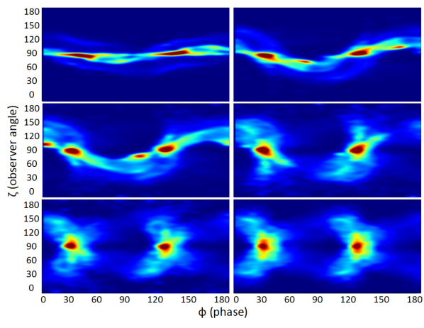
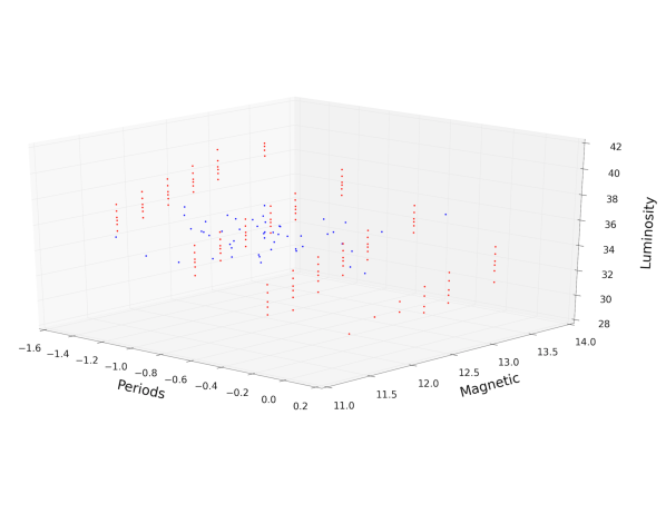
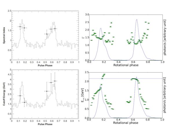
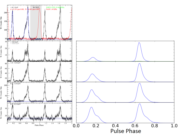
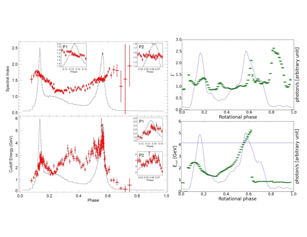
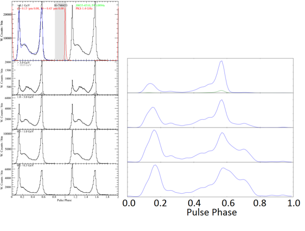
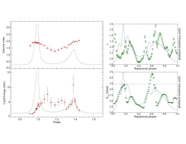
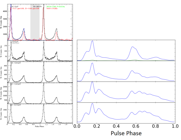
We show some figures discussed above illustrating general model properties and the data/model comparison. For the latter, the first figure for each pulsar shows the observed and model profile and the superimposed phase resolved spectra for $\Gamma$ and $E_{cut}$. The second figure shows the evolution of the observed and model light curve in the energy bins: $100MeV\div 300MeV$, $0.3GeV\div 1$ GeV, $1GeV\div 3$ GeV, $>3$ GeV, $>10$ GeV. On the right are the FIDO predictions, on the left the data.

Appendix A Vela - J0835-4510

The Vela pulsar has $P=0.089s$ and $B=3.4\cdot 10^{12}G$. The $\Delta=0.43$, the peaks “half-height width” is $0.003$ and $0.005$. The spectrum has $E_{cut}=3.0$ GeV, $\Gamma=1.5$ and the flux observed is $9.1\cdot 10^{-9}\,\rm erg/(s\cdot cm^{2})$.
The model candidate has period $P=0.1s$ and $B=4\cdot 10^{12}G$. It is for $\alpha=60^{\circ}$, $\zeta=50^{\circ}$, $\sigma=10\Omega$. The $\Delta=0.42$, the peaks “half-height width” is $0.06$ and $0.07$ where the accuracy is $\pm 0.03$ due to the smoothing. Our candidate has $E_{cut}=4.1$ GeV, $\Gamma=1.4$ and a flux of $1.9\cdot 10^{-9}\,\rm erg/(s\cdot cm^{2})$.

Figure 9.— Phase resolved spectra for Vela. Left panels: data from DeCesar (2013). Right panels: model candidate light curves (blue) and model spectral index (top) and $E_{cut}$ (bottom) (green) as a function of pulsar phase. The horizontal blue line marks the $E_{cut}$ of the phase-resolved spectrum.

Figure 10.— Light curve energy evolution for Vela. Left: Observed light curve in various energy bands, as noted, from (Abdo et al., 2013). Right: Model light curves for the same energy ranges as the data.

Appendix B Crab - J0534+2200

The Crab pulsar has $P=0.033s$ and $B=3.8\cdot 10^{12}G$. The $\Delta=0.40$, the peaks “half-height width” is $0.04$ and $0.10$. The spectrum has $E_{cut}=4.2$ GeV, $\Gamma=1.9$ and the flux observed is $1.3\cdot 10^{-9}\,\rm erg/(s\cdot cm^{2})$.
The model candidate has period $P=0.03s$ and $B=4\cdot 10^{12}G$. It is for $\alpha=75^{\circ}$, $\zeta=63^{\circ}$, $\sigma=30\Omega$. The $\Delta=0.41$, the peaks “half-height width” is $0.04$ for the first peak where the accuracy is $\pm 0.03$ due to the smoothing. The candidate’s second peak is too broad or too low. Our candidate has $E_{cut}=3.4$ GeV, $\Gamma=1.3$ and a flux of $1.6\cdot 10^{-9}\,\rm erg/(s\cdot cm^{2})$.

Figure 11.— Phase resolved spectra for Crab. Left panels: data from DeCesar (2013). Right panels: model candidate light curves (blue) and model spectral index (top) and $E_{cut}$ (bottom) (green) as a function of pulsar phase.

Figure 12.— Light curve energy evolution for Crab. Left: Observed light curve in various energy bands, as noted, from (Abdo et al., 2013). Right: Model light curves for the same energy ranges as the data.

Appendix C J1952+3252

J1952 has $P=0.04s$ and $B=0.5\cdot 10^{12}G$. The $\Delta=0.48$, the peaks “half-height width” is $0.04$ and $0.1$. The spectrum has $E_{cut}=2.5$GeV, $\Gamma=1.5$ and the flux observed is $1.4\cdot 10^{-10}\,\rm erg/(s\cdot cm^{2})$.
The model candidate has period $P=0.03s$ and $B=0.5\cdot 10^{12}G$. It is for $\alpha=75^{\circ}$, $\zeta=85^{\circ}$, $\sigma=10\Omega$. The $\Delta=0.5$, the peaks “half-height width” is $0.06$ and $0.06$ where the accuracy is $\pm 0.03$ due to the smoothing. Our candidate has $E_{cut}=2.2$ GeV, $\Gamma=1.4$ and a flux of $7.4\cdot 10^{-11}\,\rm erg/(s\cdot cm^{2})$.

Figure 13.— Phase resolved spectra for J1952+3252. Left panels: data from Abdo et al. (2010a). Right panels: model candidate light curves (blue) and model spectral index (top) and $E_{cut}$ (bottom) (green) as a function of pulsar phase.

Figure 14.— Light curve energy evolution for J1952+3252. Left: Observed light curve in various energy bands, as noted, from (Abdo et al., 2013). Right: Model light curves for the same energy ranges as the data.

References

- Abdo et al. (2009) Abdo, A. A., Ackermann, M., Atwood, W. B., et al. 2009, ApJ, 696, 1084
- Abdo et al. (2010a) Abdo, A. A., Ajello, M., Antolini, E., et al. 2010a, ApJ, 720, 26
- Abdo et al. (2010b) Abdo, A. A., Ackermann, M., Ajello, M., et al. 2010b, ApJ, 712, 1209
- Abdo et al. (2013) Abdo, A. A., Ajello, M., Allafort, A., et al. 2013, ApJS, 208, 17
- Arons (1983) Arons, J. 1983, ApJ, 266, 215
- Atwood et al. (2009) Atwood, W. B., Abdo, A. A., Ackermann, M., et al. 2009, ApJ, 697, 1071
- Bai & Spitkovsky (2010) Bai, X.-N., & Spitkovsky, A. 2010, ApJ, 715, 1282
- Cerutti et al. (2014) Cerutti, B., Philippov, A., Parfrey, K., & Spitkovsky, A. 2014, ArXiv e-prints, arXiv:1410.3757
- Chen & Beloborodov (2014) Chen, A. Y., & Beloborodov, A. M. 2014, ApJ, 795, L22
- Cheng et al. (1986) Cheng, K. S., Ho, C., & Ruderman, M. 1986, ApJ, 300, 500
- Contopoulos & Kalapotharakos (2010) Contopoulos, I., & Kalapotharakos, C. 2010, MNRAS, 404, 767
- Daugherty & Harding (1982) Daugherty, J. K., & Harding, A. K. 1982, ApJ, 252, 337
- Daugherty & Harding (1996) —. 1996, ApJ, 458, 278
- DeCesar (2013) DeCesar, M. 2013, PhD thesis, University Of Maryland
- Goldreich & Julian (1969) Goldreich, P., & Julian, W. H. 1969, ApJ, 157, 869
- Gruzinov (1999) Gruzinov, A. 1999, ArXiv Astrophysics e-prints, astro-ph/9902288
- Harding & Muslimov (2011) Harding, A. K., & Muslimov, A. G. 2011, ApJ, 743, 181
- Harding et al. (2008) Harding, A. K., Stern, J. V., Dyks, J., & Frackowiak, M. 2008, ApJ, 680, 1378
- Jackson (2001) Jackson, J. D. 2001, Classical Electrodynamics, 3rd ed. (Wiley)
- Kalapotharakos & Contopoulos (2009) Kalapotharakos, C., & Contopoulos, I. 2009, A&A, 496, 495
- Kalapotharakos et al. (2012a) Kalapotharakos, C., Contopoulos, I., & Kazanas, D. 2012a, MNRAS, 420, 2793
- Kalapotharakos et al. (2014) Kalapotharakos, C., Harding, A. K., & Kazanas, D. 2014, ApJ, 793, 97
- Kalapotharakos et al. (2012b) Kalapotharakos, C., Harding, A. K., Kazanas, D., & Contopoulos, I. 2012b, ApJ, 754, L1
- Kalapotharakos et al. (2012c) Kalapotharakos, C., Kazanas, D., Harding, A., & Contopoulos, I. 2012c, ApJ, 749, 2
- Komissarov (2006) Komissarov, S. S. 2006, MNRAS, 367, 19
- Li et al. (2012) Li, J., Spitkovsky, A., & Tchekhovskoy, A. 2012, ApJ, 746, 60
- Lyubarskii (1996) Lyubarskii, Y. E. 1996, A&A, 311, 172
- Muslimov & Harding (2004) Muslimov, A. G., & Harding, A. K. 2004, ApJ, 606, 1143
- Pétri (2012a) Pétri, J. 2012a, MNRAS, 424, 2023
- Pétri (2012b) —. 2012b, MNRAS, 424, 605
- Philippov & Spitkovsky (2014) Philippov, A. A., & Spitkovsky, A. 2014, ApJ, 785, L33
- Pierbattista et al. (2012) Pierbattista, M., Grenier, I. A., Harding, A. K., & Gonthier, P. L. 2012, A&A, 545, A42
- Pierbattista et al. (2014) Pierbattista, M., Harding, A. K., Grenier, I. A., et al. 2014, ArXiv e-prints, arXiv:1403.3849
- Romani & Watters (2010) Romani, R. W., & Watters, K. P. 2010, ApJ, 714, 810
- Romani & Yadigaroglu (1995) Romani, R. W., & Yadigaroglu, I.-A. 1995, ApJ, 438, 314
- Spitkovsky (2006) Spitkovsky, A. 2006, ApJ, 648, L51
- Tang et al. (2008) Tang, A. P. S., Takata, J., Jia, J. J., & Cheng, K. S. 2008, ApJ, 676, 562
- Tchekhovskoy et al. (2013) Tchekhovskoy, A., Spitkovsky, A., & Li, J. G. 2013, MNRAS, 435, L1
- Timokhin & Arons (2013) Timokhin, A. N., & Arons, J. 2013, MNRAS, 429, 20
- Uzdensky & Spitkovsky (2014) Uzdensky, D. A., & Spitkovsky, A. 2014, ApJ, 780, 3