Hydrogen Reionization in the Illustris universe

Abstract

Hydrodynamical simulations of galaxy formation such as the Illustris simulations have progressed to a state where they approximately reproduce the observed stellar mass function from high to low redshift. This in principle allows self-consistent models of reionization that exploit the accurate representation of the diffuse gas distribution together with the realistic growth of galaxies provided by these simulations, within a representative cosmological volume. In this work, we apply and compare two radiative transfer algorithms implemented in a GPU-accelerated code to the $106.5\,{\rm Mpc}$ wide volume of Illustris in postprocessing in order to investigate the reionization transition predicted by this model. We find that the first generation of galaxies formed by Illustris is just about able to reionize the universe by redshift $z\sim 7$, provided quite optimistic assumptions about the escape fraction and the resolution limitations are made. Our most optimistic model finds an optical depth of $\tau\simeq 0.065$, which is in very good agreement with recent Planck 2015 determinations. Furthermore, we show that moment-based approaches for radiative transfer with the M1 closure give broadly consistent results with our angular-resolved radiative transfer scheme. In our favoured fiducial model, 20% of the hydrogen is reionized by redshift $z=9.20$, and this rapidly climbs to 80% by redshift $z=6.92$. It then takes until $z=6.24$ before 99% of the hydrogen is ionized. On average, reionization proceeds ‘inside-out’ in our models, with a size distribution of reionized bubbles that progressively features regions of ever larger size while the abundance of small bubbles stays fairly constant.

1 Introduction

Figure 1: Projected slices of thickness $7.1\,{\rm cMpc}$ through the binned gas and temperature fields of the $106.5\,\mathrm{cMpc}$ wide Illustris simulation at redshift $z=7$, just before the externally applied UV background raises the temperature of the diffuse gas (the unit ‘cMpc’ stands for comoving Mpc). The left-hand panel shows the gas density field, with overlaid circles giving the locations of galaxies identified at this time by the group finder algorithm SUBFIND (Springel et al., 2001). The right-hand panel gives the corresponding mass-weighted temperature field; the heated regions around the galaxies are caused by shocks associated with virialization and feedback-driven outflows. In turn, the high temperature there leads to collisional ionization of the gas.

The cosmic microwave background (CMB) radiation was released when the Universe recombined at a redshift of $z\sim 1100$, leaving behind only a tiny residual free electron fraction. Yet in the present Universe, it is well established that the intergalactic medium (IGM) is highly ionized, as is inferred from the absence of Gunn & Peterson (1965) troughs in the absorption spectra of nearby quasars. Hence there must have been an ‘epoch of reionization’ (EoR) sometime in between, where photons emitted by stars and possibly quasars ionized the intergalactic hydrogen again (for reviews see Barkana & Loeb, 2001; Fan et al., 2006a; Morales & Wyithe, 2010). This is believed to first happen to hydrogen at $z\sim 7-10$, with helium being ionized considerably later at $z\sim 3$ (Schaye et al., 2000; McQuinn et al., 2009) by the harder radiation of quasars.

Observations of distant quasars show unambiguously that reionization was complete not much later than $z=6$ (Fan et al., 2006b). Observations of Lyman-$\alpha$ emitters indicate rapid changes in their abundance at somewhat higher redshift (e.g. Ouchi et al., 2010; Kashikawa et al., 2011; Caruana et al., 2014). Together with the relatively high optical depth to scattering on free electrons inferred from CMB observations (Bennett et al., 2013; Planck Collaboration et al., 2014) and the discovery of early galaxies at $z\sim 7$ and higher (Bouwens et al., 2011; Pentericci et al., 2011; Oesch et al., 2014), this suggests that reionization likely started considerably earlier than $z\sim 7$. The duration of the transition process, and the nature of the source population ultimately responsible for reionization, remain however subject of much observational and theoretical research.

A particularly exciting prospect is that an observational breakthrough in this field may be imminent, in particular through a direct mapping of the EoR with 21-cm observations (see Zaroubi, 2013, for a recent review). This has not yet been achieved, but impressive progress towards this goal has recently been made (e.g. Dillon et al., 2014; Parsons et al., 2014), and future instruments such as the Square Kilometer Array (SKA) or the James Webb Space Telescope (JWST) promise to revolutionize our understanding of the early universe, and of reionization in particular.

Numerous theoretical models for cosmic reionization have been constructed, often based on semi-analytic models of the reionization process or simple radiative transfer postprocessing of dark matter simulation outputs. Furlanetto et al. (2004) developed an excursion set approach to reionization that has seen widespread use in analytic and semi-numerical models of reionization (e.g. Alvarez & Abel, 2007; Zahn et al., 2011; Mesinger et al., 2011; Raičević et al., 2011; Battaglia et al., 2013). Many different numerical algorithms for direct radiative transfer simulations have also been developed over the years, in most cases however based on static density fields derived from dark matter only simulations or from simplified hydrodynamic simulations (e.g. Sokasian et al., 2001; Ciardi et al., 2003; Iliev et al., 2006; McQuinn et al., 2007; Zahn et al., 2007; Croft & Altay, 2008; Trac et al., 2008; Aubert & Teyssier, 2010; Ahn et al., 2012).

Recently, full radiation hydrodynamics simulations that follow cosmic reionization and structure formation simultaneously and self-consistently have become possible. These calculations can in principle account for radiative feedback processes on forming galaxies, for example from inhomogeneous photoionization heating. Pioneering work of this type has been presented by Gnedin (2000), but only in recent years it has become possible to study approximately representative cosmological volumes in this way (e.g. Petkova & Springel, 2011a; Paardekooper et al., 2013).

Some of the most advanced studies of this kind include the simulations recently presented by Norman et al. (2015) and So et al. (2014), who use full radiation hydrodynamics simulations of cosmic structure formation on a uniform grid. A fixed spatial grid resolution does however not allow a proper resolution of internal galaxy structure, which compromises the ability of the simulations to reliably predict the build up of stellar mass. To remedy this problem, Gnedin (2014) and Gnedin & Kaurov (2014) employ adaptive mesh refinement techniques and simulate galaxy formation in cosmological volumes with high spatial and mass resolution. Similar work has recently been presented by Pawlik et al. (2015), based on hydrodynamical SPH simulations coupled self-consistently to the radiative transfer scheme TRAPHIC (Pawlik & Schaye, 2008). However neither group evolves the simulations significantly past the EoR (let alone to $z=0$) due to the high computational cost involved, so it is not yet clear whether these simulation models would also yield a plausible present-day galaxy population.

This body of theoretical works has made it clear that the source population primarily responsible for reionization is most likely star-forming small galaxies at high redshift. While so-called Pop-III stars may boost the high redshift photon production rate, the overall contribution of these “first star” sources is likely only of secondary importance (Paardekooper et al., 2013; Wise et al., 2014). Similarly, another potential source of ionizing photons, active galactic nuclei (AGN), is not expected to be critical at high redshift due to their large mean separation (Hopkins et al., 2007; Faucher-Giguère et al., 2009) and still fairly limited cumulative luminosity. Instead, it is often argued that small proto-galaxies, with stellar masses just around $10^{4}\,{\rm M}_{\odot}$ or even lower may dominate the ionizing budget (Paardekooper et al., 2013). Ahn et al. (2012) showed that these mini halos alone can not complete reionization, but significantly contribute towards an earlier onset of reionization and thus enhance the optical depth towards the last scattering surface. These small halo mass systems are further assisted by suggestions that the escape fraction may strongly rise towards small halo masses, as inferred by Wise et al. (2014) based on radiation hydrodynamics simulation of faint high redshift galaxies. Using this finding in a semi-analytic model for reionization, Wise et al. (2014) have also demonstrated that the first galaxies may plausibly constitute the reionizing sources, yielding an optical depth consistent with Planck Collaboration et al. (2014) without exceeding the UV emissivity constraints by the Ly-$\alpha$ forest.

It is interesting however to note that the cosmic star formation history inferred from observations is predicted to rapidly decline towards high redshift (e.g. Ellis et al., 2013). This is also expected (Hernquist & Springel, 2003) and desirable on theoretical grounds (Scannapieco et al., 2012), because simulation models of galaxy formation need to resort to an extremely efficient suppression of high-redshift star formation in order to successfully describe present-day galaxy properties (e.g. Stinson et al., 2013). A very low level of high redshift star formation is however quite the opposite of what seems necessary to explain early reionization and the comparatively high optical depth inferred from CMB experiments. This tension makes it difficult to attribute reionization entirely to young galaxies with more or less ordinary stellar populations. In $\Lambda$CDM models with low normalization $\sigma_{8}$, or in alternative warm dark matter cosmologies, this problem is further exacerbated (Yoshida et al., 2003a, b), whereas in certain non-standard dark energy models that shift structure growth to earlier times, for example ‘early dark energy’ (Wetterich, 2004; Grossi & Springel, 2009), it may be alleviated.

Recently, cosmological hydrodynamic simulations of galaxy formation such as the Illustris (Vogelsberger et al., 2014b) or Eagle (Schaye et al., 2015) projects have advanced to a state where they produce realistic galaxy populations simultaneously at $z=0$ and at high redshifts, throughout a representative cosmological volume. This is achieved with coarse sub-resolution treatments of energetic feedback processes that regulate star formation, preventing it from exceeding the required low overall efficiency. Ideally the process of reionization should be coupled dynamically to such a galaxy formation model. However, running several such reionization simulations for different escape fraction parameterizations at the resolution and size of Illustris would be computationally very expensive. Thus we have here reverted to study reionization in post processing only. This approach is not as self-consistent as the most recent generation of full radiation-hydrodynamics simulations of galaxy formation (Gnedin, 2014; Norman et al., 2015; Pawlik et al., 2015), but it can take advantage of a successful description of the evolving source population and the intervening gas distribution down to low redshift.

An important manifestation of feedback are galactic winds and outflows that substantially modify the distribution of the diffuse gas in the circumgalactic medium (CGM) and the IGM. This in turn also influences the gas clumping and the recombination in models of cosmic reionization. It thus becomes particularly interesting to test whether detailed models of galaxy growth such as Illustris are in principle also capable of delivering a successful description of cosmic reionization, and if so, what assumptions are required to achieve such a success.

This is exactly the goal of this paper. We use a sequence of snapshots with high time resolution of the high-resolution Illustris simulation and combine them with a radiative transfer scheme that is capable of accurately evolving ionizing radiation for an arbitrary number of sources. We are particularly interested in the question of whether the star formation history predicted by Illustris can reionize the universe early enough to be consistent with observational constraints, and how the reionization transition proceeds in detail in this scenario. Because we have implemented two different radiative transfer methods, we can also evaluate how well they intercompare, thereby providing an estimate for systematic uncertainties related to these radiative transfer methods. We also explicitly test the impact and accuracy of the often adopted reduced speed of light approximation.

This work is structured as follows. In Section 2, we introduce the Illustris simulation and our different radiative transfer schemes that we use to follow cosmic reionization. We then turn to a discussion of our primary results in Section 3. In Section 4, we analyse numerical caveats such as resolution dependence or systematic effects due to different radiative transfer approximations and discuss our findings. This is followed by our conclusions in Section 5.

2 Methods

2.1 The Illustris simulation

Recently, Vogelsberger et al. (2014b) introduced the Illustris simulation suite, an ambitious attempt to follow cosmological hydrodynamics and the feedback processes associated with galaxy formation in a sizable region of the universe. The highest resolution simulation of the project employed $2\times 1820^{3}$ particles and cells in a box 106.5 Mpc across, yielding a mass resolution of $1.26\times 10^{6}\,{\rm M}_{\odot}$ in the baryons, and $6.26\times 10^{6}\,{\rm M}_{\odot}$ in the dark matter. The cosmology adopted is given by $\Omega_{m}=0.2726$, $\Omega_{0}=0.7274$, $\Omega_{b}=0.0456$, $\sigma_{8}=0.809$, $n_{s}=0.963$, and $H_{0}=70.4\,{\rm km\,s^{-1}Mpc^{-1}}$, which is consistent with the most recent determinations from WMAP9 and Planck. The simulations employed the moving-mesh code AREPO (Springel, 2010), which is well-suited to applications in cosmic structure formation.

The physics model employed by Illustris includes radiative cooling, metal enrichment based on 9 elements, star formation, stellar evolution and mass return, supernova feedback by means of a kinetic wind feedback, and black hole growth and associated feedback processes in a quasar- and radio-mode. We refer to Vogelsberger et al. (2013) and Torrey et al. (2014) for a description of the full details and basic tests of the model. A number of different studies have analysed structure formation in Illustris, making it clear that many basic properties of the observed galaxy populations are approximately reproduced by the simulation model. This in particular includes constraints on the stellar mass function at different epochs (Vogelsberger et al., 2014a; Genel et al., 2014), the morphologies and spectra of galaxies (Torrey et al., 2015), the colors of satellite systems (Sales et al., 2015), the stellar halos of galaxies (Pillepich et al., 2014), the nature of high redshift, compact galaxies (Wellons et al., 2015), the galaxy-galaxy merger rate (Rodriguez-Gomez et al., 2015), the kinematics and metal abundance of damped Lyman-alpha absorbers (Bird et al., 2015), or the evolution of the black hole mass density and quasar luminosity function (Sijacki et al., 2015). The galaxy formation predictions by Illustris are hence in broad agreement with observations, which adds additional motivation to ask whether they at the same time yield a plausible reionization history.

A self-consistent treatment of the UV background using radiative transfer was however not included in Illustris, as this is still beyond reach in such large cosmological simulations that are evolved to low redshift. Instead, an external, spatially uniform and time-dependent UV background was imposed based on the model of Faucher-Giguère et al. (2009), and dense gas is self-shielded from UV background radiation using a prescription derived from Rahmati et al. (2013). A coarse treatment of an AGN proximity effect was included where accreting AGNs modify the ionization balance of gas in their environment (Vogelsberger et al., 2013). In this work, we therefore aim to study reionization through postprocessing of the Illustris simulation, making use of the significant number of output dumps (more than 128, with an output spacing as in the Aquarius project, Springel et al., 2008) stored for the calculation. This allows us to take the temporal information about the growth of cosmic structures into account, avoiding the simplification of a static density field often adopted in past work. Another advantage of Illustris is the reasonably large box size of 106.5 Mpc. While a still larger volume would clearly be desirable, studies of cosmic variance of reionization have suggested that $\sim 100\,h^{-1}\mathrm{Mpc}$ corresponds to the minimum box size required to obtain a reliable mean reionization history (Mesinger & Furlanetto, 2007; Iliev et al., 2014). The volume available in Illustris falls slightly short here, but is approximately still sufficient for hydrogen reionization. Studying HeII reionization with Illustris would be more problematic however due to the incomplete sampling of bright and rare quasars.

2.2 Radiative transfer

The governing equation of radiation transfer is the Boltzmann equation for the photon distribution function,

$$\frac{\partial f_{\gamma}}{\partial t}+\frac{\partial}{\partial\boldsymbol{x}}\left(\frac{c}{a}\boldsymbol{n}f_{\gamma}\right)=\left.\frac{\partial f_{\gamma}}{\partial t}\right|_{\rm sources}-\left.\frac{\partial f_{\gamma}}{\partial t}\right|_{\rm sinks},$$ (1)

with cosmological scale factor $a$ and speed of light $c$. The function $f_{\gamma}(\boldsymbol{x},\boldsymbol{n},\nu,t)$ describes the number density of photons of frequency $\nu$ at time $t$, propagating in the direction of the normal vector $\boldsymbol{n}$. In the following, we will replace the frequency dependence by one effective frequency bin that accounts for all hydrogen ionizing photons, for simplicity. This can in principle be straightforwardly generalized to multiple frequency bins, as is necessary, for example, to also treat helium reionization. In equation (1), we ignore the redshifting of ionizing photons which is justified if photons are destroyed in ionization events shortly after their creation.

Solving equation (1) in full generality is very difficult, hence a large variety of approximation methods for cosmological radiative transfer have been developed, each with different advantages and shortcomings that ultimately dictate the regimes where they are applicable. Many radiative transfer schemes are based on the idea of characteristics (Mihalas & Mihalas, 1984), where the optical depth is individually integrated along rays between different computational cells. As this operation quickly becomes extremely costly many different techniques have been developed to accelerate the calculations, for example by using short-characteristics (e.g. Nakamoto et al., 2001), or by hierarchically splitting rays (Abel & Wandelt, 2002; Trac & Cen, 2007). Ray-tracing schemes are particularly well suited for dealing with a small number of isolated sources, and in that sense are ideal for following the growth of an isolated ionized region around a point source (Abel et al., 1999). However, the reionization problem involves a large number of sources (all the stars in a large number of galaxies), favouring the use of other methods.

One popular approach is to take moments of the radiative transfer equation, leading to an evolution equation for the mean specific intensity that needs to be closed with an estimate of the local Eddington tensor (Gnedin & Abel, 2001; Aubert & Teyssier, 2008; Petkova & Springel, 2009; Finlator et al., 2009). The simplest variant of this approach is flux-limited diffusion (FLD) of radiation (Levermore & Pomraning, 1981; Turner & Stone, 2001), which works particularly well in the optically thick regime but may fail badly in situations where the optical depth is low and shadowing might be important. Better accuracy can be obtained in moment-based approaches when the local Eddington tensor can be estimated with reasonable accuracy. This is attempted, for example, in the optically thin variable Eddington tensor (OTVET) approximation of Gnedin & Abel (2001), or by invoking other simple approximations such as the so-called M1-closure (Levermore, 1984; Aubert & Teyssier, 2008).

More general radiative transfer such as Monte Carlo methods (e.g. Maselli et al., 2003; Nayakshin et al., 2009) may also be invoked, but their computational cost is comparatively large making it difficult to avoid a high level of noise in large-scale simulated radiation fields. The TRAPHIC approach of Pawlik & Schaye (2008) improves on this by restricting the transport of photon packets to a finite set of angular cones, while retaining the flexibility of the Monte Carlo scheme. A conceptually similar idea is followed in the radiation advection scheme of Petkova & Springel (2011b), where the radiation field is directly discretized in angular space and transported with a conservative advection solver on an unstructured grid.

In our work here, we consider two different numerical methods to solve the advection part of the radiation transport, described by the left hand side of equation (1). The first method is the cone-based advection method proposed by Petkova & Springel (2011b), and the second method is a simpler moment-based approach where the M1 closure for the Eddington tensor is used (Aubert & Teyssier, 2008; Rosdahl et al., 2013). This allows us to assess how strongly fundamental differences in the numerical radiative transfer approximation affect the predicted reionization transition, thereby yielding an estimate for this contribution to the systematic uncertainties in theoretical EoR predictions.

2.3 Cone-based advection method

In the cone based method introduced by Petkova & Springel (2011b), the angular dependence of the distribution function $f_{\gamma}$ is discretized in cones of equal opening angle. We use the HEALPIX tessellation scheme (Górski et al., 2005) to subdivide the unit sphere, giving $N_{\mathrm{pix}}=12\times 4^{n}$ cones of equal solid angle, where $n$ is an integer parameter determining the resolution level. The spatial dependence can be discretized using either a structured or unstructured mesh. As we are mostly interested in volume-weighted effects of reionization (such as the volume filling factor of ionized gas) and want to efficiently exploit GPUs as computational accelerators we adopt a Cartesian grid in this work. This leaves us with $N_{\mathrm{pix}}$ photon fields, $f_{l}\left(\boldsymbol{x}_{i,j,k}\right)$, at grid coordinates $\boldsymbol{x}_{i,j,k}$, with $f_{\gamma}=\sum f_{l}$ being the total angle-integrated intensity.

Leaving the source terms aside for the moment (which are treated in an operator-split fashion), the cone-based method solves a hyperbolic advection equation,

$$\frac{\partial f_{l}}{\partial t}+\frac{\partial}{\partial\boldsymbol{x}}\left(\frac{c}{a}\boldsymbol{n}_{l}f_{l}\right)=0,$$ (2)

for each of the angular-decomposed photon fields $f_{l}$. The principal transport direction $\boldsymbol{n}_{l}$ of cone $l$ is set by the HEALPIX tessellation of the unit sphere. However, to make sure that the entire cone of each tile is illuminated homogeneously and that the transport does not excessively collimate the radiation into an angle smaller than the prescribed angular resolution, $\boldsymbol{n}_{l}$ is obtained by taking

$$\boldsymbol{n}^{\prime}=-\frac{\nabla f_{\gamma}}{\left|\nabla f_{\gamma}\right|},$$ (3)

and additionally, if this direction should fall outside of a cone with center $\boldsymbol{\tilde{n}}_{l}$ and opening angle $\phi_{\mathrm{max}}=\sqrt{4/N_{\mathrm{pix}}}$, it is projected back inside that cone. Here $\boldsymbol{\tilde{n}}_{l}$ is the geometric center of the $l^{\rm th}$ HEALPIX cell. In other words, the advection direction is constrained to lie within the cone but otherwise tries to reduce gradients in the photon intensity across the cone, thereby ensuring a homogenous illumination of the cone.

We typically integrate the above transport equations using a reconstructed piecewise constant photon intensity field combined with an upwind scheme to determine the photon flux between cells. We use explicit time integration and hence need to restrict the timestep to something of order $h/c$, where $h$ is the cell radius and $c$ the speed of light. This leads to quite small timesteps. This could be mitigated by invoking a reduced speed of light approximation (Gnedin & Abel, 2001), but as we discuss in section 4.3 we have not used this here to avoid any inaccuracies that can be introduced by this approximation.

2.4 Moment method with M1 closure

For comparison with the angular resolved transport scheme, we also implemented a moment based advection scheme. Here the radiative transfer equation is discretized by taking the first two moments of equation (1):

$$\frac{\partial N}{\partial t} +\nabla\boldsymbol{F}=0,$$ (4)

$$\frac{\partial\boldsymbol{F}}{\partial t} +c^{2}\nabla\mathbf{P}=0,$$ (5)

where the photon density $N$, the flux vector $\boldsymbol{F}$, and the photon pressure tensor ${\mathbf{P}}$ have been introduced. Solving this system of equations requires a closure for the radiation pressure tensor $\mathbf{P}$. The simplest closure is to assume an isotropic pressure, which yields the family of flux-limited diffusion methods (Levermore & Pomraning, 1981). Another possibility is the OTVET approximation where a preferred local streaming direction of photons is estimated based on the source locations and their strengths (Gnedin & Abel, 2001). More accurate estimates of a variable Eddington tensor (VET) may for example be obtained by employing a special short-characteristics method to estimate the local Eddington tensor (Davis et al., 2012; Jiang et al., 2014).

An alternative is the M1 method, where a fully local closure is used instead (Levermore, 1984; Aubert & Teyssier, 2008). This greatly simplifies the computations because information about the surrounding regions does not explicitly have to be taken into account. The photon pressure tensor of the M1 closure can be parametrized as:

$$\mathbf{P}=\left(\frac{1-\xi}{2}\mathbf{I}+\frac{3\xi-1}{2}\boldsymbol{n}\otimes\boldsymbol{n}\right)N,$$ (6)

with

$$\boldsymbol{n}=\frac{\boldsymbol{F}}{\left|\boldsymbol{F}\right|},\quad\xi=\frac{3+4f^{2}}{5+2\sqrt{4-3f^{2}}},\quad f=\frac{\left|\boldsymbol{F}\right|}{cN},$$ (7)

and identity matrix $\mathbf{I}$. Here $f$ essentially determines how directed the flux is, interpolating between the two limiting cases of radiation diffusion and photon streaming. The parameter $\xi$ varies smoothly from $\frac{1}{3}$ to $1$ between these cases. In the case of $\xi=\frac{1}{3}$, which occurs for an undirected flux, the result is isotropic advection. The other limit of $\xi=1$ corresponds to fully directed transport with one dominant propagation direction.

While in practice the M1 closure often produces surprisingly accurate results, it is easy to construct situations where it fails. For example, one obvious shortcoming occurs when two light beams directly encounter each other from opposing directions. As the photon field is essentially described by M1 as a collisional fluid with a restricted form for the local Eddington tensor, a ‘scattering’ at the beam intersection point is unavoidable, resulting in an unphysical propagation direction. Nevertheless, one can hope that in many practical applications such inaccuracies occur sufficiently rarely that the overall results are still reliable. Whether or not this is really the case is problem dependent and needs ultimately be tested by comparing with more accurate techniques that are based on different approximations, something that we also pursue in this work.

2.5 Ionization network and time integration

The evolution of the ionization state of hydrogen is given by the following system of equations:

$$\frac{{\rm d}n_{\gamma}}{{\rm d}t} =-c\sigma n_{\rm H}xn_{\gamma}+\left[\alpha_{\mathrm{A}}(T)-\alpha_{\mathrm{B}}(T)\right]n^{2}_{\rm H}\left(1-x\right)^{2},$$ (8)

$$\frac{{\rm d}xn_{\mathrm{H}}}{{\rm d}t} =\alpha_{\mathrm{A}}(T)n^{2}_{\rm H}\left(1-x\right)^{2}-\beta(T)n^{2}_{\rm H}x(1-x)-c\sigma n_{\rm H}xn_{\gamma},$$ (9)

with the hydrogen number density $n_{\mathrm{H}}$ , the frequency averaged ionization cross section $\sigma$, the number density of ionizing photons $n_{\gamma}$ and the neutral hydrogen fraction $x$. The case A and case B recombination rates $\alpha_{\mathrm{A}}$ and $\alpha_{\mathrm{B}}$ and collisional ionization rate $\beta$ are taken from Hui & Gnedin (1997). The chemical network is complemented by source terms in the thermal energy evolution describing cooling and photoionization heating:

$$\frac{{\rm d}u}{{\rm d}t}=\epsilon_{\gamma}c\sigma n_{\rm H}xn_{\gamma}-{\cal C}(T),$$ (10)

where $\epsilon_{\gamma}$ is the average gain in thermal energy per ionization event. The cooling rate ${\cal C}(T)$ includes cooling due to recombination, collisional ionization, collisional excitation and Compton cooling by scattering on CMB photons.

We solve the chemical network following the method outlined in Rosdahl et al. (2013). First, the photon number $n_{\gamma}$ is updated by an implicit Euler step, then the temperature $u$ and finally the ionization state $x$. Each partial update step is implicit in the already updated quantities and the currently updated one. The full radiative transfer equation (1) is then solved by Strang-like operator splitting, computing first the left hand side for half a time step (advection), then applying the source and sink terms, and finally completing the timestep by another half advection step. The two advection half steps themselves are solved by dimensional splitting.

In our cone-based advection method, we usually use the $n=1$ HEALPIX tessellation level with $N_{\mathrm{pix}}=48$ pixels. Due to the large number of photon fields the computations are demanding in memory as well as in computational power. To speed up our simulations, we are employing GPUs, an approach similar in spirit to Aubert & Teyssier (2010). We use a uniform Cartesian mesh which makes our algorithm ideal for GPU computing, as this leads to a regular memory access pattern and facilitates the use of groups of threads with the same execution path. Details of our GPU implementation will be described elsewhere (Bauer et al., in preparation).

2.6 Reionization in post processing

In this work, we study the progress of cosmic reionization by following the time-resolved evolution of the density field and the source population of the Illustris simulation in postprocessing. The unstructured Voronoi mesh that stores the baryon distribution in the simulation outputs needs to be rebinned onto a regular Cartesian mesh to allow use of our GPU-based code. To this end, we assign the mass of each Voronoi cell onto the density grid using a spline-kernel assignment. This yields a less noisy and smoother density field than obtained, e.g., by using a clouds-in-cells (CIC) or nearest-grid-point (NGP) assignment kernel (Hockney & Eastwood, 1981). The actual density field used in our reionization calculation is then continuously updated by linearly interpolating in time between the two nearest binned density grids available in $\log a$ space, where $a=1/(1+z)$ is the cosmological scale factor. The Illustris outputs are spaced roughly 65 Myrs apart at the relevant redshift $z\sim 6$, allowing us to bin the density field in total 35 times between redshift $z=21.8$ and $z=4.9$. Using a set of small subboxes cut out from Illustris and stored with much higher time-resolution we have checked that the sparser time resolution of the main outputs is still reasonably accurate. It shifts the completion of reionization towards slightly earlier times, but the uncertainty in our results is still dominated by the parametrization of the escape fraction. Initially we start with a uniform temperature field with $T=100\,\mathrm{K}$ and then follow the temperature evolution using equation (10), ignoring the intrinsic temperature evolution of the underlying Illustris simulation. We note that in this paper we consider hydrogen reionization only.

2.7 Escape fraction

Overview of radiative transfer simulation models
Name	Resolution	$f_{0}$	$\kappa$	Advection method
V1_X_CONE	$256^{3}$ …$512^{3}$	$0.04$	$4$	Cone based method
V5_X_CONE	$256^{3}$ …$512^{3}$	$0.04$	$3.6$	Cone based method
C2_X_CONE	$256^{3}$ …$512^{3}$	$0.2$	$0$	Cone based method
V1_X_M1	$256^{3}$ …$1024^{3}$	$0.04$	$4$	M1 method
V5_X_M1	$256^{3}$ …$1024^{3}$	$0.04$	$3.6$	M1 method
C2_X_M1	$256^{3}$ …$1024^{3}$	$0.2$	$0$	M1 method

Table 1: Overview of the different radiation transfer calculations performed for this study. We carried out runs with a resolution ranging from $256^{3}$ up to $1024^{3}$ cells, which is indicated by replacing the placeholder ‘X’ with the number of cells per dimension in the actual run name. We compare different escape fraction parameterizations, characterized by $f_{0}$ and $\kappa$. The three different choices we adopted for this are labeled ‘V1’, ‘V5’ and ‘C2’ in the simulation names. Finally, for each of the models we compare two different advection schemes for the radiation, one based on the M1 closure relation, the other on an explicit discretization of the solid angle (‘cone based’) .

Of all ionizing photons emitted by stars, only a fraction $f_{\mathrm{esc}}$ reaches the IGM, while the other photons are absorbed by the denser interstellar medium (ISM) or by dust. In principal, the escape fraction depends on individual halo properties like halo mass or dust content. Unfortunately, only little is known about the real values of the escape fractions, especially at high redshifts, making this parameter one of the primary uncertainties in studying the EoR. However, theoretical models have started to constrain the escape fraction, albeit with large systematic uncertainties. For example, the simulations of Wise et al. (2014) suggest a sharp increase of the escape fraction towards smaller masses, reaching $50\%$ at halo masses of $10^{7}\,{\rm M}_{\odot}$.

The simplest model is evidently to adopt a globally constant escape fraction that is the same for all galaxies at a given epoch. This is what we shall assume here, because one may well argue that in light of the many other uncertainties adopting a more complicated model would not be justified (see also the discussion in Pawlik et al., 2015). As a default choice for the constant escape fraction model we have considered $f_{\mathrm{esc}}=0.2$ (C2 model). This almost certainly constitutes an overestimate for low redshift galaxies, but is perhaps not overly optimistic at high redshift.

Besides such a globally constant escape fraction, we also consider an evolution of the $f_{\mathrm{esc}}$ value with time. To this end, we use the model of Kuhlen & Faucher-Giguère (2012) who proposed an evolution of the escape fraction as a function of redshift according to:

$$f_{\mathrm{esc}}=\min\left[1,f_{0}\left(\frac{1+z}{5}\right)^{\kappa}\right].$$ (11)

Our default choices for the parameters $f_{0}$ and $\kappa$ are $f_{0}=0.04$ and $\kappa=4$, implying a rise of the escape fraction with redshift (V1 model). We have also calculated results for a variety of other fiducial parameter choices as well. For an overview see Table 1.

We stress again that the escape fraction is essentially a free parameter in our treatment. Its interpretation is complicated by the fact that the absorbing ISM is not totally absent in our reionization simulations. It is just severely underesolved, and thus some part of the boost in recombination rates due to a highly clumped environment is missing. However, photons are still consumed for (repeatedly) ionizing the material in these high density regions. Unresolved small galaxies and thus missing UV photons might be compensated by a slightly larger escape fraction than otherwise would be needed.

2.8 Source modelling

Figure 2: Time evolution of the total ionizing luminosity resulting for our different escape fraction models. The model with a constant escape fraction (blue lines) tracks the shape of the cosmic star formation history. Our default models with a redshift dependent escape fraction are given by the green and red lines. For comparison, we also include the ionizing luminosity implied by the quasars included in our simulation (dashed black line), adopting a simple conversion of quasar accretion rate to ionization radiation output. This demonstrates that the quasar contribution picks up too late to cause the initial hydrogen reionization, but it may play a role in keeping the universe ionized at later times, as well as for completing late-time helium reionization.

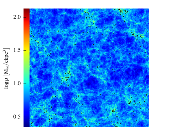
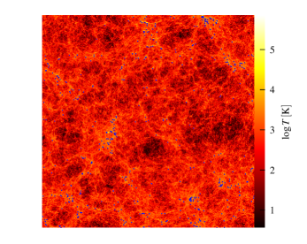
The main source of ionizing photons considered in our model is ordinary stellar populations in young stars, which arguably appear to be the most likely source responsible for reionization. In this work we are mainly interested in testing this hypothesis based on directly adopting the stellar populations forming in the Illustris simulation. Their ionizing luminosities as a function of stellar age and metallicity are taken from STARBURST-99 (Leitherer et al., 1999). Figure 1 gives a visual impression of the binned gas density field in Illustris at $z=7$, and of the clustered galaxy population that represents our source population. Because the local ionization rate can change on much shorter timescales than the density, we bin the luminosity field with much finer time resolution than the density field. In our default set-up, we binned it 200 times during the duration of the reionization simulation including the actual birth time of the stellar sources. The actual luminosity used in the simulation to integrate the source terms is then again interpolated in $\log a$ space from this large grid of luminosity density fields. The ionizing luminosity of a single stellar source is always distributed in a photon conserving way to the radiation grids. The assignment of the luminosity is done using a CIC interpolation scheme.

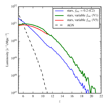
The ionizing sources we have at our disposal from the main Illustris simulation are related to the star formation rate and black hole accretion rate densities. The corresponding time evolution of the net ionizing luminosity density is shown in Figure 2, together with different scenarios for the escaping luminosity according to our escape fraction models. The blue line shows our constant escape fraction model (C2 model), while the green line is our default model for a time-varying escape fraction (V1 model). The red line (V5 model) represents a variable escape fraction model with a different value for the exponent $\kappa$ than in the V1 model. These models rapidly rise for some time, but at around a redshift of $z\simeq 8$, the escaping radiation actually reaches a maximum and then starts to slowly decline again. Here the strong decrease of the escape fraction from $1$ to $0.04$ marginally over-compensates the further increase of the star formation density and the raw ionizing luminosity. We note that the maximum coincides with the epoch where we expect most of the hydrogen to be reionized.

An alternative source of ionizing radiation is in principle provided by AGNs. We assume a bolometric AGN luminosity described by

$$L_{\mathrm{bol}}^{\mathrm{AGN}}=\left(1-\epsilon_{\mathrm{f}}\right)\tilde{\epsilon}_{\mathrm{r}}\dot{M}_{\mathrm{BH}}c^{2},$$ (12)

with a radiative efficiency of $\epsilon_{\mathrm{r}}=0.2$ and an energy fraction of $\left(1-\epsilon_{\mathrm{f}}\right)=0.95$ available for radiation. The luminosity is converted into a rate of ionizing photons assuming a parameterized AGN SED (Korista et al., 1997) equal to

$$f^{\mathrm{AGN}}(\nu)=\nu^{\alpha_{\mathrm{UV}}}\exp\left(-\frac{h\nu}{kT_{\mathrm{BB}}}\right)\exp\left(-\frac{10^{-2}\mathrm{Ryd}}{h\nu}\right)+a\nu^{\alpha_{\mathrm{x}}},$$ (13)

with a suppression of the UV component at a temperature of $T_{\mathrm{BB}}=10^{6}\,\mathrm{K}$, a UV component slope of $\alpha_{\mathrm{UV}}=-0.5$ and an X-ray component slope of $\alpha_{\mathrm{X}}=-1$. To obtain an approximation for the maximum contribution to reionization, we assume an escape fraction of $f_{\mathrm{esc,AGN}}=1$. For comparison, we show the AGN ionizing luminosity as a dashed black line in Figure 2. The AGN contribution only becomes relevant at around $z=6$, but by then most of the hydrogen must already be ionized, making it unlikely that AGNs are significantly contributing to the initial EoR transition. However, they might play a role in keeping the universe ionized at a later time, and almost certainly are important for completing helium reionization at lower redshift, thanks also to their harder spectrum. As we only study hydrogen reionization, in the following only stellar emission is considered as sources of ionizing photons.

3 Simulation results

An overview of the various reionization simulations carried out in this work is given in Table 1. To examine resolution dependences, we computed several of our models with grid resolutions of up to $1024^{3}$ cells. We considered two different models with a time-variable escape fraction and contrasted them with one model with a fixed escape fraction. In order to asses the impact of different radiative transfer methods we performed most of our simulations both with our default cone-based approach as well as with the moment-based method with M1 closure.

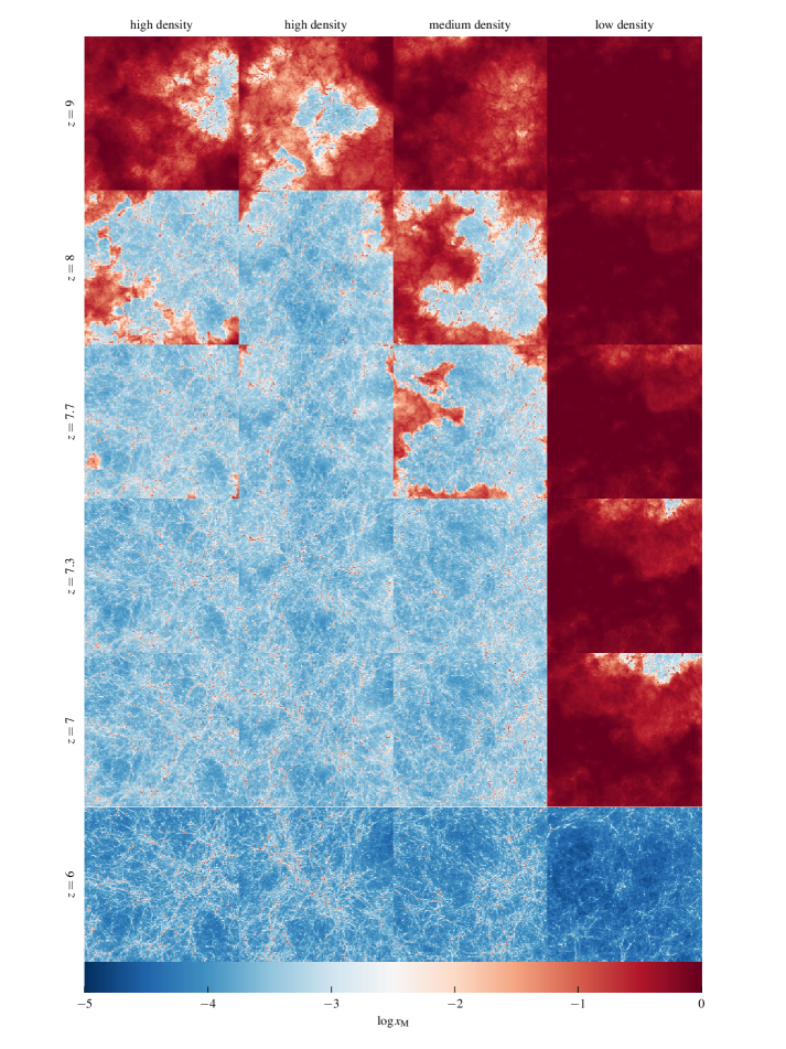
The progress of reionization in different environments is visually shown in Figure 3, where we compare two regions around very massive halos with a more average environment around a typical medium-sized halo, and an underdense region. The different projections show the four regions at six different output times. Reionization starts inside the most massive halos first, and then quickly ionizes the surrounding regions. Compared to such a high-density environment, the onset of reionization is considerably delayed around a medium mass halo. More drastically, the underdense region only begins to be reionized once the denser regions have almost completed their reionization transition. The visual impression is thus qualitatively consistent with an inside-out reionization scenario in which halos in high-density regions are affected first and lower density voids are reionized rather late, for the most part after overdense gas been reionized (Razoumov et al., 2002). This contrasts with suggestions that low density regions are reionized quite early and only then the reionization fronts progress to ionize filaments and gas in halos (Gnedin, 2000).

Figure 3: Progression of reionization as seen in the neutral hydrogen fraction in slices through selected sub-volumes in Illustris, each with a side-length of $21.3\,{\rm cMpc}$. Each column shows the time evolution of a different, randomly selected environment in our V1_1024_M1 model; the two columns on the left correspond to an average density higher than the mean, the other columns have medium and low mean density, as labeled. Each row gives a different redshift, from $z=9$ (top) to $z=6$ (bottom).

3.1 Reionization history

Figure 4: The ionization history for different escape fraction parameterizations. The upper panel shows the evolution of the volume weighted ionization fraction (solid lines rising to low redshift) and the neutral hydrogen fraction (lines dropping towards low redshift), as a function of redshift. For comparison, observational constraints by Fan et al. (2006b) are shown as symbols with error bars. The lower panel shows the ratio between mass- and volume-weighted ionization fractions $\left(1-x_{\mathrm{M}}\right)/\left(1-x_{\mathrm{V}}\right)$ for the different models.

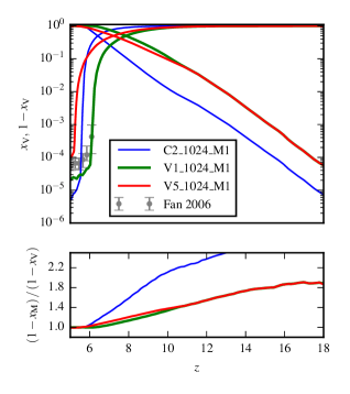
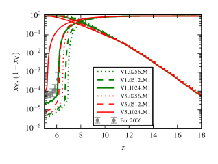
In the upper panel of Figure 4, we show the volume weighted ionization fraction $1-x_{\mathrm{V}}$ as a function of time for three of our high-resolution radiative transfer calculations. We see a rapid, exponential rise at high redshift, and an approach to unity at around $z\simeq 6-8$. The end of reionization and the rapid phase transition to a reionized universe is better visible in displaying the neutral fraction $x_{\mathrm{V}}$, which is also included in the figure. For comparison, we also show observational constraints derived by Fan et al. (2006b) from quasar absorption lines (symbols with error bars). Especially our model V1_1024_M1 reproduces the suggested end of reionization in these data quite well, although the residual neutral fraction comes out slightly low.

In the lower panel of Figure 4, we consider the evolution of the ratio between mass- and volume-weighted ionization fractions, $\left(1-x_{\mathrm{M}}\right)/\left(1-x_{\mathrm{V}}\right)$. This quantity is the average density of the ionized hydrogen compared to the average hydrogen density of the full box:

$$\frac{1-x_{\mathrm{M}}}{1-x_{\mathrm{V}}}=\frac{V_{\mathrm{tot}}}{M_{\mathrm{tot}}}\frac{\left(1-x_{\mathrm{M}}\right)M_{\mathrm{tot}}}{\left(1-x_{\mathrm{V}}\right)V_{\mathrm{tot}}}=\frac{1}{\langle\rho\rangle_{\mathrm{tot}}}\frac{M_{\mathrm{ionized}}}{V_{\mathrm{ionized}}}=\frac{\langle\rho\rangle_{\mathrm{ionized}}}{\langle\rho\rangle_{\mathrm{tot}}}.$$ (14)

This ratio stays at or above unity for all time, which can be interpreted as a signature of an inside-out character of reionization (Iliev et al., 2006). Overdense environments around our sources ionize first, so that the ionized volume is always overdense on average. Interestingly, the evolution of the mean overdensity of ionized regions with time also differs for our different escape fraction models. The run assuming a constant escape fraction model starts reionization later but then progresses somewhat more rapidly. This model maintains the highest value of $\left(1-x_{\mathrm{M}}\right)/\left(1-x_{\mathrm{V}}\right)$ for most of the simulated timespan. Here reionization is particularly biased to overdense regions and is stuck there for a comparatively long time, until the final reionization transition occurs on a short timescale and the IGM at mean density is ionized as well. Interestingly, even though the variable escape fraction models show some variety in the time of the onset of reionization and the remaining neutral fraction, the evolution of $\left(1-x_{\mathrm{M}}\right)/\left(1-x_{\mathrm{V}}\right)$ is still rather similar among these models. They begin reionization earlier and thus generally have low mean overdensities of the ionized volume at any given time.

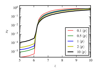
That the character of the reionization process is best described as an inside out transition can be seen in more detail in Figure 5, where the time evolution of the average neutral fraction is shown for regions of a fixed given overdensity. Highly overdense regions start to become ionized quite early on, assisted by collisional ionization in virialized halos. As a result, the reionization process for high density regions is also considerably less sudden than for lower density gas. After reionization is essentially completed, the behavior however reverses; now overdense regions show on average a final ionization degree that is considerably lower than for lower density regions. This can be understood as a result of the higher recombination rate in the denser regions, shifting the equilibrium value of the ionized fraction in a given UV background. Generally speaking, we find that denser regions start to ionize earlier but keep a higher neutral fraction than underdense regions.

Reionization is clearly not an instantaneous transition but requires a certain amount of time. It is hence interesting to characterize the epoch of reionization not only with a single redshift but also to ask how long the duration to a reionized universe takes. To this end we define the duration $\Delta z$ as the interval in redshift space during which the volume-weighted neutral fraction drops from $80\%$ to $20\%$. Our fiducial model V1_1024_M1 leads to an extent of $\Delta z=2.28$ for the epoch of reionization, corresponding to a timespan of $\Delta t=251.2\,\mathrm{Myr}$ for this period. The V5_1024_M1 model shows a slightly longer duration of reionization with $\Delta z=2.61$ and $\Delta t=341.3\,\mathrm{Myr}$. Reionization lasts only over a span of $\Delta z=1.13$ or $\Delta t=190.0\,\mathrm{Myr}$ in our C2_1024_M1 model. Thus our models with a variable escape fraction show a more extended epoch of reionization compared to the model with a constant escape fraction. In the models with a variable escape fraction, the ionizing luminosity is initially higher, but once most of the ionizing luminosity has become available, the variable escape fraction gradually begins to limit the amount of escaping UV radiation, resulting in a more prolonged epoch of reionization.

Figure 5: Time evolution of the neutral hydrogen fraction at given gas overdensities. Each of the lines shows the result for a small density range around a nominal comoving density threshold, as labeled, for our model V1_1024_M1. We see that the ionization of dense gas begins earlier, but this gas also ends up with a higher residual neutral fraction once reionization is completed.

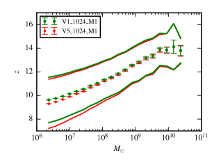
One can also ask whether galaxies of different stellar masses are all ionized at the same time, or whether there are significant systematic trends of the mean reionization epoch as a function of galaxy size. To this end, we have considered the sample of all $z=6$ galaxies in Illustris and then checked at what redshift the average ionized fraction in a sphere of radius $150\,{\rm kpc}$ around them (taking their $z=6$ positions) reached 50% for the first time. The results of this analysis are shown in Figure 6, binned as a function of stellar mass. There is a clear trend for an earlier reionization around more massive galaxies. Interestingly, the spread in the reionization times slightly increases towards smaller stellar masses, indicating that dwarf galaxies are expected to show larger diversity in their reionization histories. Also, these low mass galaxies are more sensitive to the adopted parametrization of the escape fraction and tend to reionize later in our $V5$ model.

Figure 6: Mean reionization redshifts of the immediate surroundings of galaxies as a function of their $z=6$ stellar masses for our highest resolution run of the V1 and V5 models. The symbols give the means in each mass bin, with the error bars showing the statistical error of the mean. The solid lines illustrate the $\pm 1\sigma$ variance in each mass bin.

3.2 UV background

Figure 7: Average photoionization rate $\Gamma$ as function of redshift for models calculated with different escape fractions and grid resolutions. For comparison, we also include two widely used theoretical models for the UV background evolution: FG09 (Faucher-Giguère et al., 2009, we show the updated version from Dec. 2011) and HM12 (Haardt & Madau, 2012). The V5_1024_M1 model is in particularly good agreement with FG09, at least for $z<10$.

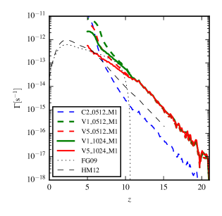
In Figure 7, we consider the time evolution of the volume averaged photoionization rate for models calculated with different escape fractions and grid resolutions, and compare to different models in the literature for the evolution of the cosmic UV background (Haardt & Madau, 2012; Faucher-Giguère et al., 2009). At high redshift, the background builds up exponentially with redshift, similar to the growth of the volume weighted ionization fraction, with an overall amplitude that varies with the escape fraction model. Our variable escape fraction models and our fixed escape fraction model bracket the scenario of HM12. Interestingly, our scenario V5_1024_M1 follows the model of Faucher-Giguère et al. (2009) very closely, except that after reionization is completed, our calculations tend to overshot the model predictions. We note that a very similar behaviour is also seen in the recent radiative transfer simulations of Pawlik et al. (2015), where this effect is even more pronounced. A more realistic variable escape fraction model than the rather simple parametrization employed might help resolving this issue.

3.3 Optical depth $\tau$

Figure 8: Cumulative optical depth for Thompson scattering on free electrons, integrated out to the redshift specified on the horizontal axis. Solid lines include electrons from doubly ionized helium (assuming that they contribute for $z<3$), while dotted lines assume hydrogen and one helium electron only. The horizontal line with $\pm 1\sigma$ uncertainty region (shaded) marks the newest 2015 constraints $\tau=0.066\pm 0.016$ by the Planck Collaboration et al. (2015). Out fiducial model V1_1024_M1 is in very good agreement with optical depth inferred from these precision measurements of the CMB. Our other models lie slightly lower, however their value is still consistent. Interestingly, the previous determination by Planck based on their first 2013 data analysis had given a considerably higher value for $\tau$. The tension with this result is now resolved.

Starting with the onset of reionization, CMB photons will Thomson scatter off the free electrons again. This effect can be quantified by measuring the cumulative optical depth $\tau$ seen by CMB photons along their path towards us. This optical depth is given by

$$\tau=c\,\sigma_{\mathrm{th}}\int^{0}_{z_{0}}n_{e}(z)\frac{\mathrm{d}t}{\mathrm{d}z}\mathrm{d}z,$$ (15)

where $\sigma_{\mathrm{th}}$ is the Thomson cross section, and $n_{e}$ the number density of free electrons. In this work, we only consider hydrogen reionization for simplicity. Given that the first ionization potential of helium is very close to the ionization potential of hydrogen, we assume that HeII is created in proportion to HII. The free electron density is then given by

$$n_{e}=\left[1+\frac{1-X}{4X}\right]\left(1-x_{\mathrm{M}}\right)n_{\rm H}\approx 1.079\,\left(1-x_{\mathrm{M}}\right)n_{\rm H},$$ (16)

where $X=0.76$ is the hydrogen mass fraction. At late times, helium reionization will eventually be completed, increasing the optical depth slightly compared to the above estimate. Adopting the common assumption that helium becomes doubly ionized at $z=3$ (e.g. Iliev et al., 2005), the free electron density increases by $\Delta n_{e}=(1-X)/(4X)\left(1-x_{\mathrm{M}}\right)n_{\rm H}\simeq 0.079\,\left(1-x_{\mathrm{M}}\right)n_{\rm H}$ compared to the estimate above, and hence the optical is enlarged by

$$\Delta\tau=c\,\sigma_{\mathrm{th}}\int^{0}_{3}\Delta n_{e}(z)\frac{\mathrm{d}t}{\mathrm{d}z}\mathrm{d}z=0.0011,$$ (17)

which is a very small correction given the other uncertainties.

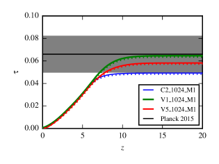
The optical depth $\tau$ for a specific reionization history can be converted into an effective reionization redshift $z_{\mathrm{reion}}$ assuming a fiducial scenario in which the reionization transition is instantaneous at this epoch. The latest WMAP9 results find a best-fit value of $\tau=0.088\pm 0.013$, corresponding to $z_{\mathrm{reion}}=10.5\pm 1.1$ (Hinshaw et al., 2013), quite a bit lower than the value of $\tau=0.17\pm 0.08$ WMAP1 had initially estimated. The results of the PLANCK mission in its 2013 data release (Planck Collaboration et al., 2014) favour a very similar, slightly larger value for the optical depth, $\tau=0.089\pm 0.032$, corresponding to an even earlier reionization redshift of $z_{\mathrm{reion}}=10.8$. However, the latest PLANCK data release of 2015 (Planck Collaboration et al., 2015) prefers a much lower optical depth of $\tau=0.066\pm 0.016$ and a corresponding redshift of reionization of $z_{\mathrm{reion}}=8.8^{+1.7}_{-1.4}$. A similar low optical depth of $\tau=0.063\pm 0.013$ has been found in Finkelstein et al. (2014) based on a UV luminosity function derived from Hubble Ultra Deep Field and Hubble Frontier Field data.

In Figure 8, we show the optical depth of our reionization simulations as a function of the integration redshift $z$ for three of our models. The most recent 2015 constraint from PLANCK is shown as a horizontal line, together with the $\pm 1\sigma$ uncertainty region (shaded). Our models with a variable escape fraction are comfortably compatible within the error bars with the 2015 Planck results. Our fiducial model V1_1024_M1 predicts an optical depth of $\tau=0.065$ which is in very good agreement with the most recent Planck 2015 data. However all of our other models prefer the low side of the range determined by Planck. Still, it is very promising that the former tension between galaxy formation simulations and optical depth inferred from CMB measurements seems nearly resolved with the 2015 Planck data. A similar finding has been reported in Robertson et al. (2015) based on Hubble observations of distant galaxies. Allowing for additional high redshift star formation could easily close the small remaining gap if needed, but we note that constraints from galaxy formation disfavour this solution. For example, Illustris already tends to overshoot estimates for the stellar mass function of small galaxies, at late and early times alike (Vogelsberger et al., 2014a; Genel et al., 2014). Resolving these problems seems to call for reduced high redshift star formation and not the opposite, highlighting the difficulty to reconcile high optical depths values from CMB experiments with detailed galaxy formation models.

3.4 Bubble size statistics

Figure 9: Distribution of the characteristics radius of ionized regions at four different redshifts, in our fiducial model V1_1024_M1. The integral over the distributions is normalized to unity for each of the measurements, and a horizontal line corresponds to equal volume fraction per logarithmic size interval. Initially, small bubbles dominate but over time the distribution shifts to ever larger bubbles until only one large region dominates.

Figure 10: The same information as in Fig. 9, except with a different normalization. Here the integral is normalized by the constant comoving box volume so that the area under the distributions gives the total ionized volume fraction. This is informative because the relative constancy of the size distributions for small bubble sizes suggests that the growing bubbles are replenished by new small bubbles just at the right rate to achieve this balance. Interestingly, the volume occupied by small bubbles stays hence roughly the same for the whole duration of reionization, even slightly beyond bubble percolation where a dominating single large ionized region forms.

Mapping the epoch of reionization more directly than possible thus far, for example through 21cm imaging, is an exciting observational prospect. Once this becomes possible with future radio telescopes such as the SKA, quantitative measures of the geometry of the ionized regions, such as their topology, promise to be a powerful probe of theoretical models for reionization. Radiation transfer models like those calculated herein are the method of choice to make the required detailed predictions about how these morphological measures evolve in time. To illustrate this, we here compute a few basic statistical measures that quantify the number and size of ionized regions as a function of time, which may also serve as a useful comparison against other theoretical reionization models.

We start by tagging cells as ionized if their ionization fraction exceeds $1-x_{\mathrm{M}}>0.5$. Based on the resulting grid of binary values, ionized regions are then identified using a friends-of-friends algorithm that links adjacent ionized cells (Iliev et al., 2006; Chardin et al., 2012). We let cells belong to the same group if they share at least one corner, or in other words, if any of the $26$ neighbours of an ionized cell is also ionized, both cells are put into the same group. For each ionized island identified in this way, we compute an effective radius as $r=\left[{3}/\left({4\pi}V\right)\right]^{1/3}$, where $V$ is the cumulative volume of the cells making up the group. Finally, we consider the distribution function $f_{V}$ of the ionized volume fraction contained in regions of a given bubble radius.

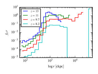
In Figure 9, we show the resulting distribution function when the convention of Zahn et al. (2007) is followed and the distribution is normalized such that

$$\int f_{V}r\,\mathrm{d}\!\log r=1,$$ (18)

i.e. we only consider the ionized volume of the box. The results show that at early times, when only a small fraction of the volume is ionized, the ionized volume is comprised of disjoint regions of characteristic size $r\simeq 2\,{\rm cMpc}$. While reionization progresses, ever larger bubbles appear, with a flat distribution as a function of size, i.e. roughly the same amount of ionized volume is contained per logarithmic interval in bubble size, up to bubble sizes of the order of $r\simeq 20\,{\rm cMpc}$. Eventually, the bubbles start to percolate and one dominating region containing a substantial fraction of the simulation volume is formed ($z=8.2$). There is then still a population of smaller ionized regions left, with a constant volume fraction per unit $\log r$ over a dynamic range of about $\sim 5$ in size.

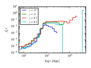
An alternative normalization for the size distribution is used in Gnedin & Kaurov (2014), who consider the whole box thus that integrating over $f_{V}$ gives the ionized volume fraction:

$$\int f^{\prime}_{V}\,r\,\mathrm{d}\!\log r=1-x_{\mathrm{V}}.$$ (19)

It is instructive to plot the corresponding distributions also with this normalization, which is shown in Figure 10. Now the area under the distribution function grows with redshift, reflecting the increase of the ionized volume fraction. Interestingly, we see in this representation that the bubble size distribution is fairly constant with time, especially for the small bubble sizes. Even though these bubbles grow individually in size with time, the fact that the abundance of bubbles of a given size stays approximately constant in time (once the first bubbles of this size have formed), suggests that small bubbles are reformed just at the right rate to compensate for the loss of bubbles of a given size due to the growth or coalescence of bubbles.

Figure 11: Degree of ionization level PDFs at different redshifts. The top panel shows the results for the V1_1024_M1 model, whereas the bottom panel is for the V5_1024_M1 model. Compare to Fig. 7, where the V1 run shows a strong upturn in the UV flux, which is here expressed as a shift of ionized cells down to $n_{\mathrm{HI}}=10^{-5}$ at around $z=5.3$, which does not happen in the V5 run.

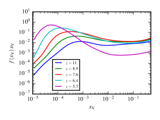
3.5 Distribution function of neutral volume fraction

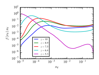
In Figure 11, we show the distribution function $f(x_{\mathrm{V}})={\rm d}V/{\rm d}x_{\mathrm{V}}$ of the volume fraction that is found at a given neutral fraction. We compare our two different variable reionization scenarios, in the form of V1_1024_M1 (top panel) and V5_1024_M1 (bottom panel), and give results for different redshifts in each case. Note that we plot $x_{\mathrm{V}}\,f(x_{\mathrm{V}})$ on the vertical axis versus the log of $x_{\mathrm{V}}$, i.e. the area under the curves is proportional to the volume fraction at the corresponding range of neutral fractions.

Progress in reionization is associated with a large increase in the volume fraction found at low neutral fractions, as is of course expected. Interestingly, the differential distribution of volume at a given neutral fraction is however fairly broad while reionization is not completed, with a peak at a characteristic neutral fraction that shifts progressively to lower values. For example, at redshifts $z\simeq 11$, most of the volume is either still neutral or at a neutral fraction of $x_{\mathrm{V}}\sim 10^{-3}$. At around redshift $z\sim 7$, the characteristic neutral fraction where most of the volume is found has dropped to $x_{\mathrm{V}}\sim 10^{-4}$. Finally, post reionization, the two models start to differ more prominently. Here V1_1024_M1 shows a low neutral fraction of $x_{\mathrm{V}}\sim 10^{-5}$ or lower for most of its volume, which corresponds also to the strong rise in the predicted UV background seen in this model in Figure 7. In contrast, the model V5_1024_M1, which shows good agreement with the UV background model of Faucher-Giguère et al. (2009) at this epoch, yields a markedly different distribution of the neutral fraction, with most of the volume having neutral fractions around $x_{\mathrm{V}}\simeq 5\times 10^{-5}$.

4 Caveats and Discussion

The accuracy and reliability of our results are influenced by many numerical aspects as well as physical uncertainties. In the following we discuss a number of these aspects, focusing primarily on those pertaining to the radiative transfer modelling itself. We note however that there are in principle additional uncertainties related, for example, to the treatment of star formation and the associated feedback processes in the underlying Illustris simulation, or to the cosmological background model that we use. These are arguably subdominant compared to the uncertainties related to the reionization calculation itself (such as escape fraction, radiative transfer solver, etc.), and in any case are beyond the scope of this paper (a discussion of the uncertainties in the galaxy formation model can be found in Vogelsberger et al., 2014a).

4.1 Reionization feedback

Due to the fact that we simulate reionization only in post-processing, any back reaction onto the gas due to photoionization heating and potentially radiation pressure is not taken into account self-consistently. The Illustris simulation assumes a uniform global UV background, hence the average back reaction on star formation due to photo-ionization is approximately accounted for, but any local modulation of the corresponding effects is of course ignored. This limitation could only be overcome by dynamically coupling the radiative transfer solver to a hydrodynamical code and doing full radiation-hydrodynamics simulations of galaxy formation. Recently, impressive progress has been made in this direction (Gnedin, 2014; Gnedin & Kaurov, 2014; Pawlik et al., 2015), but the achieved cosmological volumes are still severely limited due to the demanding computational cost of radiative transfer, and in general, these calculations have not been evolved to redshift $z=0$, and thus it is unclear whether they are successfully reproducing the observed galaxy population.

Besides photo-heating, the ionizing radiation of young stars could also exert significant feedback effects through radiation pressure, particularly in dusty gas where infrared radiation may be trapped (Murray et al., 2010; Hopkins et al., 2012; Agertz et al., 2013). However, the effectiveness of this mechanism is debated, with a number of recent studies arguing that photo-heating is likely the dominant feedback channel on the scale of galaxies, with radiation pressure being comparatively unimportant (Sales et al., 2014; Rosdahl et al., 2015). We thus consider the omission of radiation pressure effects in our reionization calculations to be comparatively unimportant.

4.2 Moment-based versus cone-based RT method

Our radiative transfer implementation supports two different transport methods, allowing us to compare them against each other with no changes in any other aspect of the modelling. In the case of the cone-based method, we have to store and process 48 radiation intensity fields, one for each advection direction. On the other hand, the moment-based M1 scheme only requires 4 fields, one for the photon number density and 3 for the flux vector. This difference makes the cone-based advection scheme much more expensive in terms of computational cost as well as in terms of (GPU) memory requirements.

Figure 12: Visual comparison of our two different radiation advection methods at two instances in time. All panels show a thin slice through the box with a side length of $21.3\,\textrm{cMpc}$. The top row compares the neutral hydrogen fraction at $z=8.5$ for the cone-based method (left) and the moment-based method with M1 closure (right). Similarly, the bottom row shows this comparison for redshift $z=8$.

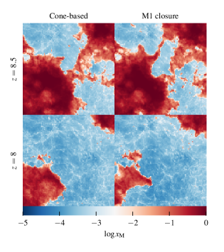
If we compare the ionization histories predicted by these different radiative transfer methods in terms of the ionized volume fraction, no appreciable differences are detected. In fact, the agreement of the evolution of the ionized volume fractions is so good that we refrain from showing the corresponding comparison in a dedicated plot. But this consistency is perhaps not too surprising. The ionization history mainly depends on the source population that injects ionizing photons, as well as on the density evolution of the gas, as the latter sensitively determines the recombination rate. Given that the photon injection rates and the density structure are exactly equal in our comparison, and given the fact that both radiative transfer algorithms are manifestly photon conserving, any difference between the cone-based and the M1-closure methods can only be induced by differences in the photon transport directions. These are apparently subtle enough that they do not matter much for global statistics of the reionization transition.

However, despite this good agreement in global averages, the two methods still show differences in the detailed morphology of the ionized bubbles when examined in detail. In Figure 12, we compare the morphology of the ionized regions around a typical galaxy at redshifts $z=8$ and $z=8.5$. While there is clearly a great deal of similarity, the detailed locations of the ionization fronts differ substantially, highlighting that the radiative transfer solvers do not behave identically after all. This is also borne out by a higher order quantitative comparison of the neutral hydrogen fraction fields predicted by the two methods. This can for example be done by computing the mass-weighted standard deviation of the difference between the neutral hydrogen densities obtained by our two radiative transfer schemes:

$$v=\mathrm{var}\left(\rho\left(x_{\mathrm{M1}}-x_{\mathrm{CONE}}\right)\right)/\left<\rho\right>.$$ (20)

For our V1_0512 models, we find that this quantity rises with decreasing redshift until a maximum of $v=0.2$ is reached at $z=7.5$. Afterwards, the full volume is quickly reionized and the variance of the difference field rapidly declines again. We note that the cone-based method should be the more accurate approach in this comparison, as it can avoid certain inaccuracies of the M1 approach, in particular when the ionization bubbles of two or more sources overlap.

4.3 How accurate is the reduced speed of light approximation?

As long as the medium is dense enough, the propagation speed of the ionization fronts is determined by the rate at which new ionizing photons arrive at the edge of neutral gas, and not how fast they get there. This motivates the idea of the so-called reduced speed of light approximation (Gnedin & Abel, 2001; Aubert & Teyssier, 2008), in which the physical value of $c$ is artificially reduced. The computational advantage of a reduced speed of light is that a much larger Courant time step is allowed in schemes where photon transport is followed with explicit time integration. Rosdahl et al. (2013) report that the reduced speed of light approximation describes the solution of Strömgren sphere well after an effective crossing time $t_{\mathrm{cross}}=r_{\mathrm{S}}/c$, where $r_{\mathrm{S}}$ is the radius of the corresponding Strömgren sphere and $c$ the (reduced) speed of light. Before $t_{\mathrm{cross}}=r_{\mathrm{S}}/c$, however, the numerical solution necessarily always falls behind the correct one. Considering the relevant time scales that have to be resolved in cosmic reionization, this yields a criterium for the maximum allowed reduction of the speed of light. The conclusion of Rosdahl et al. (2013) is that there is not much room for applying the reduced speed of light approximation if accurate reionization simulations of the IGM are desired.

Figure 13: Impact of the reduced speed of light approximation on the evolution of the neutral and ionized volume fractions. Reducing the speed of light by a factor of 10 (blue line) or 100 (red line) relative to our default calculation with a physical speed of light (green line) causes a later reionization of the universe.

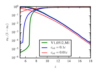
It is interesting to use our independent radiative transfer code to check this assessment. In Figure 13, we show the impact of the reduced speed of light on the obtained reionization history, based on a reduction of the physical speed of light by a factor of 10 or 100, respectively. Consistently with the findings of Rosdahl et al. (2013), the reduction of the speed of light leads to a significant delay in the resulting epoch of reionization, amounting to $\Delta z\sim 1-1.5$ for the factor of 10 reduction, and much larger for a factor of 100. The size of this error unfortunately implies that this numerical trick can induce unacceptably large distortions in the reionization predictions, hence we have refrained from using it throughout the study.

4.4 Clumping factors

Figure 14: Clumping factor of the gas computed in different ways. The upper solid line shows the intrinsic clumping factor of all non star-forming gas (with density below the star formation threshold), based on the Voronoi tessellation of the Illustris simulation volume. The dotted line gives the intrinsic clumping factor of all the gas in the simulation. For comparison, we also show the clumping factor of all the non star-forming gas when this is obtained for different mesh resolutions after mapping the simulation volume to a grid with fixed spatial resolution.

Figure 15: Gas clumping factors measured for gas below a certain characteristic gas overdensity. The left-hand panel shows $C_{20}$, with the solid black line giving the result for the actual Voronoi tessellation used in the Illustris simulation for the hydrodynamical calculations. The other solid lines give the corresponding result for the binned density field when grids with resolution from $256^{3}$ to $1024^{3}$ are used, as labeled. The right-hand panel gives the same results for $C_{100}$, where instead a density threshold of 100 times the mean baryonic density is adopted. For reference, we also show fitting models by Finlator et al. (2012, F12) and (Pawlik et al., 2009, P09), which give the clumping factor of ionized gas or gas below a overdensity threshold of 100 (their $z\sim 7.5$ reionization case), respectively.

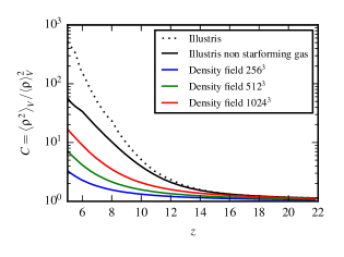
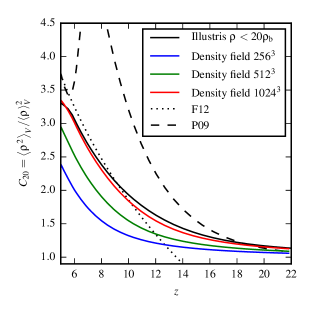
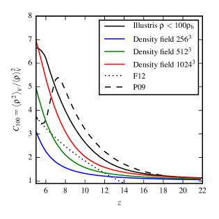
The degree of gas clumping is a critical factor in models of reionization, as it directly determines the recombination rate and hence the amount of photons required to reionize the universe and to keep it ionized. Full hydrodynamical simulations of galaxy formation are a particularly powerful tool to realistically predict the non-linear density structure of the gas, and hence to quantify the gas clumping. In Figure 14, we show the full clumping factor $C$ of all the gas, defined in the standard way as

$$C=\frac{\left<\rho^{2}\right>}{\left<\rho\right>^{2}},$$ (21)

where the averages are volume averages for the full simulation box. The black lines represent the clumping factor obtained directly from the Voronoi cells of the underlying Illustris simulation, which is hence accounting for all structure resolved by the more than 6 billion cells of the simulation. We give results for the complete density field (dotted line) as well as for cells constrained to not lie on the effective equation of state of star forming gas (solid black line). The former result includes the collapsed gas that corresponds to the ISM and is star-forming, whereas in the latter this phase is excluded. The clumping factor is obviously much higher when this star-forming gas is included, but as the sub-grid model used by Illustris glosses over the true multi-phase nature of the ISM, the resulting clumping factor for all the gas is still an underestimate. However, we are here really only interested in the non-starforming gas, because the recombinations and absorptions inside the star forming regions are collectively accounted for by the escape fraction, which in part may be viewed as parameterizing our ignorance of the detailed gas structure on ISM scales.

The solid red, green and blue lines in Fig. 14 show the clumping factor of all gas after binning it on radiation transfer grids with different resolution. Clearly, even for the $1024^{3}$ grid we loose almost a factor of two in the total clumping due to the smoothing of this grid. However, as cosmic reionization is a volume filling process and the densest gas occupies only a tiny fraction of the value, it makes more sense to refer the escape fraction to a somewhat lower density threshold than the star-formation threshold. We are hence really interested in the clumping factor of gas up to some limited overdensity value, for example up to 20 or 100 times the mean baryonic density. Since both of these fiducial values have been used in the literature, we show in Figure 15 our results for $C_{20}$ and $C_{100}$ (in the left- and right-hand panels, respectively), where only gas cells which have a density of at most $20\times\rho_{\mathrm{b}}$ or $100\times\rho_{\mathrm{b}}$ have been included, respectively, with $\rho_{\mathrm{b}}=\Omega_{\rm b}\rho_{\mathrm{crit}}$ denoting the mean baryon density. As before, we show results for the underlying Voronoi tessellation as well as reionization grids between $256^{3}$ and $1024^{3}$ resolutions. Note that in these plots a linear scale for the clumping factor has been used.

Our high resolution radiative transfer grid underpredicts the $C_{\rm 20}$ clumping a bit due to the smoothing effects of the binning, but the effect is minor. The situation is a bit worse if one also wants to get the correct clumping factor for gas up to an overdensity of 100. Here some of this additional clumping is not resolved by the $1024^{3}$ grid, as the results in the right-hand panel of Fig. 15 show. Given the trend with increasing resolution, using a $2048^{3}$ grid instead (which we unfortunately cannot carry out due to memory constraints on the GPU system we have presently access to) should however be able to fully recover the $C_{100}$ clumping of this gas. As we discuss in more detail below, this resolution problem for the $C_{100}$ quantity affects cosmic reionization however only mildly and is hence comparatively benign.

It is interesting to compare our clumping factors with those inferred from other works. Finlator et al. (2012) have pointed out that different definitions of the clumping factor can produce substantial differences in the results. It is thus important to base any such comparison on the same definition, which sometimes corresponds to considering the clumping of all the gas below a certain density threshold (to separate collapsed and diffuse gas), or to restricting the evaluation of the clumping factor to ionized gas. Note that the latter depends both on the detailed reionization model and the gas distribution. To get a sense of how well the gas distributions compare, it is thus arguably best to compare the total gas clumping factor. For the Illustris simulation at $z=8$, we measure for the clumping of the non-starforming gas $10.2$, slightly higher than the value reported by Finlator et al. (2012). However, our value is significantly higher than the total gas clumping factor of $C\sim 3$ at $z=8$ reported by Jeeson-Daniel et al. (2014), which makes it considerably easier to achieve reionization in their model. When the baryon density is restricted to lie below an overdensity of 100, we find a clumping factor of about 4 at $z=8$, somewhat larger than what was found in Pawlik et al. (2009) for their models reionizing at or before $z=9$, but a bit lower than their model reionizing at $z=7.5$. For a yet lower overdensity threshold of 20, Wise et al. (2014) report a value of 6.5, which is above our measurement of $\simeq 2.4$ for $C_{20}$ at redshift $z=8$. This likely reflects the higher mass resolution of their simulation, which has a boxsize of just $1\,{\rm Mpc}$, but it could also be affected by the different feedback models in the two simulations.

4.5 Spatial resolution and convergence

Because the recombination rate depends nonlinearly on the density in a cell, the smoothing of density fluctuations (for example as a result of binning) causes an underestimate of recombination events and hence biases reionization towards higher redshift. Our results for the clumping factor indicate that our radiative transfer calculations clearly suffer from this effect to some degree. However, it is not obvious whether the size of the bias is quantitatively significant in the end, because the clumping of the volume-filling gas (which has comparatively low overdensity) is captured well by our high-resolution grid. If reionization would mostly occur ‘outside-in’, with low density regions ionized early, one may hope that this is already sufficient for allowing converged predictions of the reionization redshift even if density peaks are washed out. However, given that our results have confirmed that dense regions tend to be ionized earlier, this may largely be wishful thinking.

Indeed, this is borne out by our convergence tests for the reionization history of models V1 and V5 shown in Figure 16. Evidently, as the resolution of the grid for the radiative transfer simulation is increased, reionization happens progressively somewhat later, as a result of the smaller degree of suppression of the true underlying clumpiness of the gas. This prevents us from achieving a formal numerical convergence for our reionization histories. We note however that full radiation hydrodynamics simulations will counter this drift by physically inducing a reduction of the clumpiness of the gas (Pawlik et al., 2009), due to the photo-heating and the resulting pressure smoothing. This effect is not included in our simulations prior to redshift $z=6$, when reionization happens due to the externally imposed UV background. We thus expect that our $1024^{3}$ and $512^{3}$ grids may well bracket the true behavior of the clumping in a self-consistent simulation with full radiation hydrodynamics. This then also means that a $2048^{3}$ calculation without taking this effect into account may well produce a less accurate result than the $1024^{3}$ grid we used.

Figure 16: Convergence study for the neutral and ionized volume fractions for our reionization simulations based on the M1 method. The green and red lines are for the two different variable escape fraction models we considered. There are significant residual trends with resolution due to the smoothing effects a coarse grid has on the clumpy gas distribution. As a result, the highest resolution simulation tends to reionize slightly later than predicted by calculations at lower resolution.

5 Conclusions

In this work, we considered only hydrogen reionization and focused on ordinary high-redshift star formation as the primary source of ionizing photons. Other populations may in principal contribute to reionization, in particular primordial population-III stars, AGNs, or exotic sources such as annihilating dark matter. While Pop-III stars may be important for the onset of reionization, most estimates for their relative contribution to global star formation suggest that neglecting them for reionization is justified. Still, accounting for them in future models would be clearly desirable, if only for completeness. Our neglect of AGN radiation for hydrogen reionization is however quite well justified because their ionizing luminosity is overwhelmed by star formation at high redshift. AGNs become important at intermediate redshifts, however, where they likely play an important role in HeII reionization.

Even with these simplifying assumptions, calculating the ionizing flux that becomes available for reionization is affected by a substantial number of uncertainties. This includes the stellar population synthesis model we have used, and in particular, the adopted stellar initial mass function, where we used a Chabrier IMF and assumed that there are no significant IMF variations as a function of environment. Another major uncertainty lies in the escape fraction, which is physically uncertain and is in large part a phenomenological parameter in our models, absorbing uncertainties due to the treatment of dense gas and the limited spatial resolution. Finally, there are also numerical limitations related to the radiative transfer solver, the finite angular and spatial resolution employed in the radiative transfer, and the lack of self-consistently accounting for local feedback effects by the radiation field.

Fortunately some of these uncertainties can be greatly reduced by matching key observables such as the total optical depth for electron scattering or the amplitude of the metagalactic ionizing UV background after completion of reionization (e.g. Faucher-Giguère et al., 2008a, b). Our radiative transfer models for Illustris then basically test whether cosmic reionization does occur for reasonable assumptions about the escape fraction, based on a galaxy population that yields a successful description of a slew of other observational data both at high and low redshift. To the extent this works, it provides reassurance for the cosmological consistency of our galaxy formation and reionization models, and it shows that they are physically meaningful. Importantly, they can hence be used to learn more about the reionization transition itself. Our main findings can be summarized as follows:

1. The star formation history predicted by the Illustris simulation combined with its high-resolution gas density field allows cosmic reionization with an optical depth of $\tau=0.065$, consistent with the latest Planck 2015 results as well as constraints from high-redshift quasars. This relies on ordinary stellar populations only, but requires optimistic assumptions for a high escape fraction at high redshift.

2. Previous tensions between the high optical depth favoured by CMB results and the low level of high redshift star formation required by successful galaxy formation models are thus essentially resolved with Planck 2015.

3. Using a suitable variable escape fraction model, we can approximately reproduce the expected UV background after reionization is completed, but most of our models tend to then overshoot the ionization rate and yield a slightly lower neutral fraction than inferred from quasar absorption lines. A fine-tuned model may plausibly yield an improved match.

4. Reionization proceeds inside out in our model, with overdense regions being ionized earlier on average than lower density regions.

5. The size distribution of ionized regions shows a remarkable constancy with time for small bubble sizes, suggesting that during reionization new small bubbles are formed roughly at the rate at which they are removed by size growth or coalescence with other regions. The characteristic size of bubbles grows with time, but there is a fairly flat distribution of sizes between $r\sim 2\,{\rm cMpc}$ and $r\sim 20\,{\rm cMpc}$ with about equal volume fraction per logarithmic size interval just before reionization is completed.

6. The duration of the reionization transition varies with the escape fraction model, and we find transition times for a drop of the neutral fraction from 80 to 20% between 190 and 340 Myr, depending on the model.

7. The distribution of volume with respect to neutral fraction is quite broad but shows a peak that progresses to ever smaller neutral fraction with time. For models that successfully match the UV background constraints after reionization, the characteristic neutral fraction is $5\times 10^{-5}$, with the lowest amount of volume found at neutral fractions of $2\times 10^{-2}$.

In future work based on our methodology it would be particularly interesting to study HeII reionization. Due to the two ionization levels of helium with different ionization thresholds, the computational cost rises by at least a factor of about three, as more spectral bins have to be tracked instead of just one for hydrogen. Additionally, a much longer physical time down to $z\sim 3$ has to be followed. This would still be possible in postprocessing with a future Illustris type simulation with a larger box size, containing an evolving AGN population including contributions from the brightest objects. Simulating this much physical time is extremely challenging for direct radiation-hydrodynamics simulations, much more so than hydrogen reionization simulations that can be stopped at $z\simeq 6$. This makes postprocessing approaches the only practical radiative transfer method to study HeII reionization in the near term.

References

- Abel & Wandelt (2002) Abel T., Wandelt B. D., 2002, MNRAS, 330, L53
- Abel et al. (1999) Abel T., Norman M. L., Madau P., 1999, ApJ, 523, 66
- Agertz et al. (2013) Agertz O., Kravtsov A. V., Leitner S. N., Gnedin N. Y., 2013, ApJ, 770, 25
- Ahn et al. (2012) Ahn K., Iliev I. T., Shapiro P. R., Mellema G., Koda J., Mao Y., 2012, ApJ, 756, L16
- Alvarez & Abel (2007) Alvarez M. A., Abel T., 2007, MNRAS, 380, L30
- Aubert & Teyssier (2008) Aubert D., Teyssier R., 2008, MNRAS, 387, 295
- Aubert & Teyssier (2010) Aubert D., Teyssier R., 2010, ApJ, 724, 244
- Barkana & Loeb (2001) Barkana R., Loeb A., 2001, Phys. Rep., 349, 125
- Battaglia et al. (2013) Battaglia N., Trac H., Cen R., Loeb A., 2013, ApJ, 776, 81
- Bennett et al. (2013) Bennett C. L., et al., 2013, ApJS, 208, 20
- Bird et al. (2015) Bird S., Haehnelt M., Neeleman M., Genel S., Vogelsberger M., Hernquist L., 2015, MNRAS, 447, 1834
- Bouwens et al. (2011) Bouwens R. J., et al., 2011, ApJ, 737, 90
- Caruana et al. (2014) Caruana J., Bunker A. J., Wilkins S. M., Stanway E. R., Lorenzoni S., Jarvis M. J., Ebert H., 2014, MNRAS, 443, 2831
- Chardin et al. (2012) Chardin J., Aubert D., Ocvirk P., 2012, A&A, 548, A9
- Ciardi et al. (2003) Ciardi B., Ferrara A., White S. D. M., 2003, MNRAS, 344, L7
- Croft & Altay (2008) Croft R. A. C., Altay G., 2008, MNRAS, 388, 1501
- Davis et al. (2012) Davis S. W., Stone J. M., Jiang Y.-F., 2012, ApJS, 199, 9
- Dillon et al. (2014) Dillon J. S., et al., 2014, Phys. Rev. D, 89, 023002
- Ellis et al. (2013) Ellis R. S., et al., 2013, ApJ, 763, L7
- Fan et al. (2006a) Fan X., Carilli C. L., Keating B., 2006a, ARA&A, 44, 415
- Fan et al. (2006b) Fan X., et al., 2006b, AJ, 132, 117
- Faucher-Giguère et al. (2008a) Faucher-Giguère C.-A., Lidz A., Hernquist L., Zaldarriaga M., 2008a, ApJ, 682, L9
- Faucher-Giguère et al. (2008b) Faucher-Giguère C.-A., Lidz A., Hernquist L., Zaldarriaga M., 2008b, ApJ, 688, 85
- Faucher-Giguère et al. (2009) Faucher-Giguère C.-A., Lidz A., Zaldarriaga M., Hernquist L., 2009, ApJ, 703, 1416
- Finkelstein et al. (2014) Finkelstein S. L., et al., 2014, preprint, (arXiv:1410.5439)
- Finlator et al. (2009) Finlator K., Özel F., Davé R., 2009, MNRAS, 393, 1090
- Finlator et al. (2012) Finlator K., Oh S. P., Özel F., Davé R., 2012, MNRAS, 427, 2464
- Furlanetto et al. (2004) Furlanetto S. R., Zaldarriaga M., Hernquist L., 2004, ApJ, 613, 1
- Genel et al. (2014) Genel S., et al., 2014, MNRAS, 445, 175
- Gnedin (2000) Gnedin N. Y., 2000, ApJ, 535, 530
- Gnedin (2014) Gnedin N. Y., 2014, ApJ, 793, 29
- Gnedin & Abel (2001) Gnedin N. Y., Abel T., 2001, New Astron., 6, 437
- Gnedin & Kaurov (2014) Gnedin N. Y., Kaurov A. A., 2014, ApJ, 793, 30
- Górski et al. (2005) Górski K. M., Hivon E., Banday A. J., Wandelt B. D., Hansen F. K., Reinecke M., Bartelmann M., 2005, ApJ, 622, 759
- Grossi & Springel (2009) Grossi M., Springel V., 2009, MNRAS, 394, 1559
- Gunn & Peterson (1965) Gunn J. E., Peterson B. A., 1965, ApJ, 142, 1633
- Haardt & Madau (2012) Haardt F., Madau P., 2012, ApJ, 746, 125
- Hernquist & Springel (2003) Hernquist L., Springel V., 2003, MNRAS, 341, 1253
- Hinshaw et al. (2013) Hinshaw G., et al., 2013, The Astrophysical Journal Supplement Series, 208, 19
- Hockney & Eastwood (1981) Hockney R. W., Eastwood J. W., 1981, Computer Simulation Using Particles
- Hopkins et al. (2007) Hopkins P. F., Richards G. T., Hernquist L., 2007, ApJ, 654, 731
- Hopkins et al. (2012) Hopkins P. F., Quataert E., Murray N., 2012, MNRAS, 421, 3522
- Hui & Gnedin (1997) Hui L., Gnedin N. Y., 1997, MNRAS, 292, 27
- Iliev et al. (2005) Iliev I. T., Scannapieco E., Shapiro P. R., 2005, ApJ, 624, 491
- Iliev et al. (2006) Iliev I. T., Mellema G., Pen U.-L., Merz H., Shapiro P. R., Alvarez M. A., 2006, MNRAS, 369, 1625
- Iliev et al. (2014) Iliev I. T., Mellema G., Ahn K., Shapiro P. R., Mao Y., Pen U.-L., 2014, MNRAS, 439, 725
- Jeeson-Daniel et al. (2014) Jeeson-Daniel A., Ciardi B., Graziani L., 2014, MNRAS, 443, 2722
- Jiang et al. (2014) Jiang Y.-F., Stone J. M., Davis S. W., 2014, ApJS, 213, 7
- Kashikawa et al. (2011) Kashikawa N., et al., 2011, ApJ, 734, 119
- Korista et al. (1997) Korista K., Baldwin J., Ferland G., Verner D., 1997, ApJS, 108, 401
- Kuhlen & Faucher-Giguère (2012) Kuhlen M., Faucher-Giguère C.-A., 2012, MNRAS, 423, 862
- Leitherer et al. (1999) Leitherer C., et al., 1999, The Astrophysical Journal Supplement Series, 123, 3
- Levermore (1984) Levermore C. D., 1984, J. Quant. Spectrosc. Radiative Transfer, 31, 149
- Levermore & Pomraning (1981) Levermore C. D., Pomraning G. C., 1981, ApJ, 248, 321
- Maselli et al. (2003) Maselli A., Ferrara A., Ciardi B., 2003, MNRAS, 345, 379
- McQuinn et al. (2007) McQuinn M., Lidz A., Zahn O., Dutta S., Hernquist L., Zaldarriaga M., 2007, MNRAS, 377, 1043
- McQuinn et al. (2009) McQuinn M., Lidz A., Zaldarriaga M., Hernquist L., Hopkins P. F., Dutta S., Faucher-Giguère C.-A., 2009, ApJ, 694, 842
- Mesinger & Furlanetto (2007) Mesinger A., Furlanetto S., 2007, ApJ, 669, 663
- Mesinger et al. (2011) Mesinger A., Furlanetto S., Cen R., 2011, MNRAS, 411, 955
- Mihalas & Mihalas (1984) Mihalas D., Mihalas B. W., 1984, Foundations of radiation hydrodynamics
- Morales & Wyithe (2010) Morales M. F., Wyithe J. S. B., 2010, ARA&A, 48, 127
- Murray et al. (2010) Murray N., Quataert E., Thompson T. A., 2010, ApJ, 709, 191
- Nakamoto et al. (2001) Nakamoto T., Umemura M., Susa H., 2001, MNRAS, 321, 593
- Nayakshin et al. (2009) Nayakshin S., Cha S.-H., Hobbs A., 2009, MNRAS, 397, 1314
- Norman et al. (2015) Norman M. L., Reynolds D. R., So G. C., Harkness R. P., Wise J. H., 2015, ApJS, 216, 16
- Oesch et al. (2014) Oesch P. A., et al., 2014, ApJ, 786, 108
- Ouchi et al. (2010) Ouchi M., et al., 2010, ApJ, 723, 869
- Paardekooper et al. (2013) Paardekooper J.-P., Khochfar S., Dalla Vecchia C., 2013, MNRAS, 429, L94
- Parsons et al. (2014) Parsons A. R., et al., 2014, ApJ, 788, 106
- Pawlik & Schaye (2008) Pawlik A. H., Schaye J., 2008, MNRAS, 389, 651
- Pawlik et al. (2009) Pawlik A. H., Schaye J., van Scherpenzeel E., 2009, MNRAS, 394, 1812
- Pawlik et al. (2015) Pawlik A. H., Schaye J., Dalla Vecchia C., 2015, MNRAS, 451, 1586
- Pentericci et al. (2011) Pentericci L., et al., 2011, ApJ, 743, 132
- Petkova & Springel (2009) Petkova M., Springel V., 2009, MNRAS, 396, 1383
- Petkova & Springel (2011a) Petkova M., Springel V., 2011a, MNRAS, 412, 935
- Petkova & Springel (2011b) Petkova M., Springel V., 2011b, MNRAS, 415, 3731
- Pillepich et al. (2014) Pillepich A., et al., 2014, MNRAS, 444, 237
- Planck Collaboration et al. (2014) Planck Collaboration et al., 2014, A&A, 571, A16
- Planck Collaboration et al. (2015) Planck Collaboration et al., 2015, preprint, (arXiv:1502.01582)
- Rahmati et al. (2013) Rahmati A., Pawlik A. H., Raičević M., Schaye J., 2013, MNRAS, 430, 2427
- Raičević et al. (2011) Raičević M., Theuns T., Lacey C., 2011, MNRAS, 410, 775
- Razoumov et al. (2002) Razoumov A. O., Norman M. L., Abel T., Scott D., 2002, ApJ, 572, 695
- Robertson et al. (2015) Robertson B. E., Ellis R. S., Furlanetto S. R., Dunlop J. S., 2015, ApJ, 802, L19
- Rodriguez-Gomez et al. (2015) Rodriguez-Gomez V., et al., 2015, MNRAS, 449, 49
- Rosdahl et al. (2013) Rosdahl J., Blaizot J., Aubert D., Stranex T., Teyssier R., 2013, MNRAS, 436, 2188
- Rosdahl et al. (2015) Rosdahl J., Schaye J., Teyssier R., Agertz O., 2015, preprint, (arXiv:1501.04632)
- Sales et al. (2014) Sales L. V., Marinacci F., Springel V., Petkova M., 2014, MNRAS, 439, 2990
- Sales et al. (2015) Sales L. V., et al., 2015, MNRAS, 447, L6
- Scannapieco et al. (2012) Scannapieco C., et al., 2012, MNRAS, 423, 1726
- Schaye et al. (2000) Schaye J., Theuns T., Rauch M., Efstathiou G., Sargent W. L. W., 2000, MNRAS, 318, 817
- Schaye et al. (2015) Schaye J., et al., 2015, MNRAS, 446, 521
- Sijacki et al. (2015) Sijacki D., Vogelsberger M., Genel S., Springel V., Torrey P., Snyder G. F., Nelson D., Hernquist L., 2015, MNRAS, 452, 575
- So et al. (2014) So G. C., Norman M. L., Reynolds D. R., Wise J. H., 2014, ApJ, 789, 149
- Sokasian et al. (2001) Sokasian A., Abel T., Hernquist L. E., 2001, New Astron., 6, 359
- Springel (2010) Springel V., 2010, MNRAS, 401, 791
- Springel et al. (2001) Springel V., White S. D. M., Tormen G., Kauffmann G., 2001, MNRAS, 328, 726
- Springel et al. (2008) Springel V., et al., 2008, MNRAS, 391, 1685
- Stinson et al. (2013) Stinson G. S., Brook C., Macciò A. V., Wadsley J., Quinn T. R., Couchman H. M. P., 2013, MNRAS, 428, 129
- Torrey et al. (2014) Torrey P., Vogelsberger M., Genel S., Sijacki D., Springel V., Hernquist L., 2014, MNRAS, 438, 1985
- Torrey et al. (2015) Torrey P., et al., 2015, MNRAS, 447, 2753
- Trac & Cen (2007) Trac H., Cen R., 2007, ApJ, 671, 1
- Trac et al. (2008) Trac H., Cen R., Loeb A., 2008, ApJ, 689, L81
- Turner & Stone (2001) Turner N. J., Stone J. M., 2001, ApJS, 135, 95
- Vogelsberger et al. (2013) Vogelsberger M., Genel S., Sijacki D., Torrey P., Springel V., Hernquist L., 2013, MNRAS, 436, 3031
- Vogelsberger et al. (2014a) Vogelsberger M., et al., 2014a, MNRAS, 444, 1518
- Vogelsberger et al. (2014b) Vogelsberger M., et al., 2014b, Nature, 509, 177
- Wellons et al. (2015) Wellons S., et al., 2015, MNRAS, 449, 361
- Wetterich (2004) Wetterich C., 2004, Physics Letters B, 594, 17
- Wise et al. (2014) Wise J. H., Demchenko V. G., Halicek M. T., Norman M. L., Turk M. J., Abel T., Smith B. D., 2014, MNRAS, 442, 2560
- Yoshida et al. (2003a) Yoshida N., Sokasian A., Hernquist L., Springel V., 2003a, ApJ, 591, L1
- Yoshida et al. (2003b) Yoshida N., Sokasian A., Hernquist L., Springel V., 2003b, ApJ, 598, 73
- Zahn et al. (2007) Zahn O., Lidz A., McQuinn M., Dutta S., Hernquist L., Zaldarriaga M., Furlanetto S. R., 2007, ApJ, 654, 12
- Zahn et al. (2011) Zahn O., Mesinger A., McQuinn M., Trac H., Cen R., Hernquist L. E., 2011, MNRAS, 414, 727
- Zaroubi (2013) Zaroubi S., 2013, in Wiklind T., Mobasher B., Bromm V., eds, Astrophysics and Space Science Library Vol. 396, Astrophysics and Space Science Library. p. 45 (arXiv:1206.0267)