Some singular minimizers in low dimensions in the calculus of variations

Connor Mooney ย andย  Ovidiu Savin Department of Mathematics, Columbia University, New York, NY 10027 cmooney@math.columbia.edu savin@math.columbia.edu
Abstract.

We construct a singular minimizing map ๐ฎ๐ฎ\bf u from โ„3superscriptโ„3\mathbb{R}^{3} to โ„2superscriptโ„2\mathbb{R}^{2} of a smooth uniformly convex functional of the form โˆซB1Fโ€‹(Dโ€‹๐ฎ)โ€‹๐‘‘xsubscriptsubscript๐ต1๐น๐ท๐ฎdifferential-d๐‘ฅ\int_{B_{1}}F(D{\bf u})\,dx.

1. Introduction

In this paper we consider minimizers of functionals of the form

(1.1) โˆซB1Fโ€‹(Dโ€‹๐ฎ)โ€‹๐‘‘xsubscriptsubscript๐ต1๐น๐ท๐ฎdifferential-d๐‘ฅ\int_{B_{1}}F(D{\bf u})\,dx

where ๐ฎโˆˆH1โ€‹(B1)๐ฎsuperscript๐ป1subscript๐ต1{\bf u}\in H^{1}(B_{1}) is a map from โ„nsuperscriptโ„๐‘›\mathbb{R}^{n} to โ„msuperscriptโ„๐‘š\mathbb{R}^{m} and F๐นF is a smooth, uniformly convex function on Mmร—nsuperscript๐‘€๐‘š๐‘›M^{m\times n} with bounded second derivatives. By a minimizer we understand a map ๐ฎ๐ฎ\bf u for which the integral above increases after we perform any smooth deformation of ๐ฎ๐ฎ\bf u, with compact support in B1subscript๐ต1B_{1}. If F๐นF satisfies these conditions then minimizers are unique subject to their own boundary condition. Moreover ๐ฎ๐ฎ\bf u is a minimizer if and only if it solves the Euler-Lagrange system

(1.2) divโ€‹(โˆ‡Fโ€‹(Dโ€‹๐ฎ))=0,divโˆ‡๐น๐ท๐ฎ0\text{div}(\nabla F(D{\bf u}))=0,

in the sense of distributions.

The regularity of minimizers of (1.1) is a well-studied problem. Morrey [Mo] showed that in dimension n=2๐‘›2n=2 all minimizers are smooth. This is also true in the scalar case m=1๐‘š1m=1 by the classical results of De Giorgi and Nash [DG1],[Na]. In the scalar case, the regularity is obtained by differentiating equation (1.2) and treating the problem as a linear equation with bounded measurable coefficients. An example of De Giorgi [DG2] shows that these techniques cannot be extended to the case mโ‰ฅ2๐‘š2m\geq 2. Another example due to Giusti and Miranda [GM2] shows that elliptic systems do not have regularity even when the coefficients depend only on ๐ฎ๐ฎ{\bf u}. On the other hand it is known that minimizers of (1.1) are smooth away from a closed singular set of Hausdorff nโˆ’p๐‘›๐‘n-p dimensional measure zero for some p>2๐‘2p>2, see [GM1], [GG]. (In fact, if F๐นF is uniformly quasi-convex then minimizers are smooth away from a closed set of Lebesgue measure zero, see Evans [E2]). However, the singular set may be non-empty. We will discuss some interesting examples below.

The main result of this paper is a counterexample to the regularity of minimizers of (1.1) when n=3๐‘›3n=3 and m=2๐‘š2m=2, which are the optimal dimensions in light of the previous results. The existence of such minimizing maps from โ„3superscriptโ„3\mathbb{R}^{3} to โ„3superscriptโ„3\mathbb{R}^{3} or from โ„3superscriptโ„3\mathbb{R}^{3} to โ„2superscriptโ„2\mathbb{R}^{2} is stated as an open problem in the book of Giaquinta (see [Gi], p. 61).

The first example of a singular minimizer of (1.1) is due to Neฤas [Ne]. He considered the homogeneous degree one map

๐ฎโ€‹(x)=xโŠ—x|x|๐ฎ๐‘ฅtensor-product๐‘ฅ๐‘ฅ๐‘ฅ{\bf u}(x)=\frac{x\otimes x}{|x|}

from โ„nsuperscriptโ„๐‘›\mathbb{R}^{n} to โ„n2superscriptโ„superscript๐‘›2\mathbb{R}^{n^{2}} for n๐‘›n large, and constructed explicitly a smooth uniformly convex F๐นF on Mn2ร—nsuperscript๐‘€superscript๐‘›2๐‘›M^{n^{2}\times n} for which ๐ฎ๐ฎ{\bf u} minimizes (1.1). Later Hao, Leonardi and Neฤas [HLN] improved the dimension to n=5๐‘›5n=5 using

(1.3) ๐ฎโ€‹(x)=xโŠ—x|x|โˆ’|x|nโ€‹I.๐ฎ๐‘ฅtensor-product๐‘ฅ๐‘ฅ๐‘ฅ๐‘ฅ๐‘›๐ผ{\bf u}(x)=\frac{x\otimes x}{|x|}-\frac{|x|}{n}I.

The values of (1.3) are symmetric and traceless, and thus lie in a nโ€‹(n+1)/2โˆ’1๐‘›๐‘›121n(n+1)/2-1 dimensional subspace of Mnร—nsuperscript๐‘€๐‘›๐‘›M^{n\times n}. ล verรกk and Yan [SY1] showed that the map (1.3) is a counterexample for n=3,m=5formulae-sequence๐‘›3๐‘š5n=3,\,m=5. Their approach is to construct a quadratic null Lagrangian L๐ฟL which respects the symmetries of ๐ฎ๐ฎ{\bf u}, such that โˆ‡L=โˆ‡Fโˆ‡๐ฟโˆ‡๐น\nabla L=\nabla F on Dโ€‹๐ฎโ€‹(B1)๐ท๐ฎsubscript๐ต1D{\bf u}(B_{1}) for some smooth, uniformly convex F๐นF on M5ร—3superscript๐‘€53M^{5\times 3}. The Euler-Lagrange system divโ€‹(โˆ‡Fโ€‹(Dโ€‹๐ฎ))=divโ€‹(โˆ‡Lโ€‹(Dโ€‹๐ฎ))=0divโˆ‡๐น๐ท๐ฎdivโˆ‡๐ฟ๐ท๐ฎ0\text{div}(\nabla F(D{\bf u}))=\text{div}(\nabla L(D{\bf u}))=0 then holds automatically. In [SY2] they use the same technique to construct a non-Lipschitz minimizer with n=4,m=3formulae-sequence๐‘›4๐‘š3n=4,\,m=3 coming from the Hopf fibration. To our knowledge, these are the lowest-dimensional examples to date.

Our strategy is different and it is based on constructing a homogenous of degree one minimizer in the scalar case for an integrand which is convex but has โ€œflat piecesโ€.

An interesting problem about the regularity of minimizers occurs in the scalar case when considering in (1.1) convex integrands F:โ„nโ†’โ„:๐นโ†’superscriptโ„๐‘›โ„F:\mathbb{R}^{n}\to\mathbb{R} for which the uniform convexity of F๐นF fails on some compact set ๐’ฎ๐’ฎ\mathcal{S}. Assume for simplicity that F๐นF is smooth outside the degeneracy set ๐’ฎ๐’ฎ\mathcal{S}, and also that F๐นF satisfies the usual quadratic growth at infinity. One key question is whether or not the gradient โˆ‡uโˆ‡๐‘ข\nabla u localizes as we focus closer and closer to a point x0โˆˆB1subscript๐‘ฅ0subscript๐ต1x_{0}\in B_{1}. In [DS] it was proved that, in dimension n=2๐‘›2n=2, the sets โˆ‡uโ€‹(Bฮตโ€‹(x0))โˆ‡๐‘ขsubscript๐ต๐œ€subscript๐‘ฅ0\nabla u(B_{\varepsilon}(x_{0})) decrease uniformly as ฮตโ†’0โ†’๐œ€0\varepsilon\to 0 either to a point outside ๐’ฎ๐’ฎ\mathcal{S}, or to a connected subset of ๐’ฎ๐’ฎ\mathcal{S}. In Theorem 1.1 below we show that this โ€œcontinuity propertyโ€ of โˆ‡uโˆ‡๐‘ข\nabla u does not hold in dimension n=3๐‘›3n=3 when the set ๐’ฎ๐’ฎ\mathcal{S} is the union of two disconnected convex sets. We remark that, as in the p๐‘p-Laplace equation, it is relatively standard (see [E1, CF]) to obtain the continuity of โˆ‡uโˆ‡๐‘ข\nabla u outside the convex hull ๐’ฎcsuperscript๐’ฎ๐‘\mathcal{S}^{c} of ๐’ฎ๐’ฎ\mathcal{S}.

Let w๐‘คw be the homogeneous degree one function

wโ€‹(x1,x2)=x22โˆ’x122โ€‹(x12+x22)=โˆ’12โ€‹rโ€‹cosโก2โ€‹ฮธ,๐‘คsubscript๐‘ฅ1subscript๐‘ฅ2superscriptsubscript๐‘ฅ22superscriptsubscript๐‘ฅ122superscriptsubscript๐‘ฅ12superscriptsubscript๐‘ฅ2212๐‘Ÿ2๐œƒw(x_{1},x_{2})=\frac{x_{2}^{2}-x_{1}^{2}}{\sqrt{2(x_{1}^{2}+x_{2}^{2})}}=\frac{-1}{\sqrt{2}}\,\,r\,\cos 2\theta,

and let u0subscript๐‘ข0u_{0} be the function on โ„3superscriptโ„3\mathbb{R}^{3} obtained by revolving w๐‘คw around the x1subscript๐‘ฅ1x_{1} axis,

u0โ€‹(x1,x2,x3)=wโ€‹(x1,x22+x32).subscript๐‘ข0subscript๐‘ฅ1subscript๐‘ฅ2subscript๐‘ฅ3๐‘คsubscript๐‘ฅ1superscriptsubscript๐‘ฅ22superscriptsubscript๐‘ฅ32u_{0}(x_{1},x_{2},x_{3})=w\left(x_{1},\sqrt{x_{2}^{2}+x_{3}^{2}}\right).

We show that u0subscript๐‘ข0u_{0} solves a degenerate elliptic equation that is uniformly elliptic away from the cone

K0={x12>x22+x32}.subscript๐พ0superscriptsubscript๐‘ฅ12superscriptsubscript๐‘ฅ22superscriptsubscript๐‘ฅ32K_{0}=\{x_{1}^{2}>x_{2}^{2}+x_{3}^{2}\}.
Theorem 1.1.

For any ฮด>0๐›ฟ0\delta>0 there exists a convex function G0โˆˆC1,1โˆ’ฮดโ€‹(โ„3)subscript๐บ0superscript๐ถ11๐›ฟsuperscriptโ„3G_{0}\in C^{1,1-\delta}(\mathbb{R}^{3}) which is linear on two bounded convex sets containing โˆ‡u0โ€‹(K0)โˆ‡subscript๐‘ข0subscript๐พ0\nabla u_{0}(K_{0}), uniformly convex and smooth away from these two convex sets, such that u0subscript๐‘ข0u_{0} is a minimizer of the functional

โˆซB1G0โ€‹(โˆ‡u0)โ€‹๐‘‘x.subscriptsubscript๐ต1subscript๐บ0โˆ‡subscript๐‘ข0differential-d๐‘ฅ\int_{B_{1}}G_{0}(\nabla u_{0})\,dx.

We use u0subscript๐‘ข0u_{0} and G0subscript๐บ0G_{0} to construct a singular minimizing map from โ„3superscriptโ„3\mathbb{R}^{3} to โ„2superscriptโ„2\mathbb{R}^{2}. Rescaling u0subscript๐‘ข0u_{0} we obtain a function u1superscript๐‘ข1u^{1} that solves an equation that is uniformly elliptic away from a thin cone around the x1subscript๐‘ฅ1x_{1} axis, and switching the x1subscript๐‘ฅ1x_{1} and x3subscript๐‘ฅ3x_{3} axes we get an analogous function u2superscript๐‘ข2u^{2}. Then ๐ฎ=(u1,u2)๐ฎsuperscript๐‘ข1superscript๐‘ข2{\bf u}=(u^{1},u^{2}) is a minimizing map for

F0โ€‹(p1,p2):=G1โ€‹(p1)+G2โ€‹(p2),assignsubscript๐น0superscript๐‘1superscript๐‘2subscript๐บ1superscript๐‘1subscript๐บ2superscript๐‘2F_{0}(p^{1},p^{2}):=G_{1}(p^{1})+G_{2}(p^{2}),

which is a convex function defined on โ„6โ‰…M2ร—3superscriptโ„6superscript๐‘€23\mathbb{R}^{6}\cong M^{2\times 3}. Notice that the Euler-Lagrange system divโ€‹(โˆ‡F0โ€‹(Dโ€‹๐ฎ))=0divโˆ‡subscript๐น0๐ท๐ฎ0\text{div}(\nabla F_{0}(D{\bf u}))=0 is de-coupled, and F0subscript๐น0F_{0} fails to be uniformly convex or smooth in certain regions. However, a key observation is that F0subscript๐น0F_{0} separates quadratically from its tangent planes when restricted to the image of Dโ€‹๐ฎ๐ท๐ฎD{\bf u}. We obtain our example by making a small perturbation of F0subscript๐น0F_{0}.

More specifically, let

u1โ€‹(x1,x2,x3)=u0โ€‹(x1/2,x2,x3),u2โ€‹(x1,x2,x3)=u1โ€‹(x3,x2,x1)formulae-sequencesuperscript๐‘ข1subscript๐‘ฅ1subscript๐‘ฅ2subscript๐‘ฅ3subscript๐‘ข0subscript๐‘ฅ12subscript๐‘ฅ2subscript๐‘ฅ3superscript๐‘ข2subscript๐‘ฅ1subscript๐‘ฅ2subscript๐‘ฅ3superscript๐‘ข1subscript๐‘ฅ3subscript๐‘ฅ2subscript๐‘ฅ1u^{1}(x_{1},x_{2},x_{3})=u_{0}(x_{1}/2,x_{2},x_{3}),\quad u^{2}(x_{1},x_{2},x_{3})=u^{1}(x_{3},x_{2},x_{1})

and let

(1.4) ๐ฎ=(u1,u2).๐ฎsuperscript๐‘ข1superscript๐‘ข2{\bf u}=(u^{1},u^{2}).

Our main theorem is:

Theorem 1.2.

The map (1.4) is a minimizer of

โˆซB1Fโ€‹(Dโ€‹๐ฎ)โ€‹๐‘‘xsubscriptsubscript๐ต1๐น๐ท๐ฎdifferential-d๐‘ฅ\int_{B_{1}}F(D{\bf u})\,dx

for some smooth, uniformly convex F:M2ร—3โ†’โ„:๐นโ†’superscript๐‘€23โ„F:M^{2\times 3}\rightarrow\mathbb{R}.

The paper is organized as follows. In Section 2 we state a convex extension lemma and the key proposition, which asserts the existence of a suitable smooth small perturbation of G0subscript๐บ0G_{0}. We then use them to prove Theorem 1.2. In Section 3 we prove the key proposition. This section contains most of the technical details. In Section 4 we prove the extension lemma and some technical inequalities needed for the key proposition. Finally, at the end of Section 4 we outline how to prove Theorem 1.1.

2. Key Proposition and Proof of Theorem 1.2

In this section we state the extension lemma and the key proposition. We then use them to prove Theorem 1.2.

The function F0subscript๐น0F_{0} defined in the Introduction is not uniformly convex in M2ร—3superscript๐‘€23M^{2\times 3}, but it separates quadratically from its tangent planes on the image of Dโ€‹๐ฎ๐ท๐ฎD\bf u which, by the one-homogeneity of ๐ฎ๐ฎ\bf u, is the two dimensional surface Dโ€‹๐ฎโ€‹(S2)๐ท๐ฎsuperscript๐‘†2D{\bf u}(S^{2}). The quadratic separation holds on this surface since G1subscript๐บ1G_{1} is uniformly convex in the region where G2subscript๐บ2G_{2} is flat and vice versa. We would like to find a uniformly convex extension of F0subscript๐น0F_{0} with the same tangent planes on Dโ€‹๐ฎโ€‹(โˆ‚B1)๐ท๐ฎsubscript๐ต1D{\bf u}(\partial B_{1}).

2.1. Extension Lemma

The extension lemma gives a simple criterion for deciding when the tangent planes on a smooth surface can be extended to a global smooth, uniformly convex function. Let ฮฃฮฃ\Sigma be a smooth compact, embedded surface in โ„nsuperscriptโ„๐‘›\mathbb{R}^{n} of any dimension.

Lemma 2.1.

Let G๐บG be a smooth function and ๐ฏ๐ฏ{\bf v} a smooth vector field on ฮฃฮฃ\Sigma such that

(2.1) Gโ€‹(y)โˆ’Gโ€‹(x)โˆ’๐ฏโ€‹(x)โ‹…(yโˆ’x)โ‰ฅฮณโ€‹|yโˆ’x|2,๐บ๐‘ฆ๐บ๐‘ฅโ‹…๐ฏ๐‘ฅ๐‘ฆ๐‘ฅ๐›พsuperscript๐‘ฆ๐‘ฅ2G(y)-G(x)-{\bf v}(x)\cdot(y-x)\geq\gamma|y-x|^{2},

for any x,yโˆˆฮฃ๐‘ฅ๐‘ฆฮฃx,\,y\in\Sigma and some ฮณ>0๐›พ0\gamma>0. Then there exists a global smooth function F๐นF such that F=G๐น๐บF=G and โˆ‡F=๐ฏโˆ‡๐น๐ฏ\nabla F={\bf v} on ฮฃฮฃ\Sigma, and D2โ€‹Fโ‰ฅฮณโ€‹Isuperscript๐ท2๐น๐›พ๐ผD^{2}F\geq\gamma I.

The idea of the proof is to first make a local extension by adding a large multiple of the square of distance from ฮฃฮฃ\Sigma. We then make an extension to all of โ„nsuperscriptโ„๐‘›\mathbb{R}^{n} by taking the supremum of tangent paraboloids to the local extension. Finally we mollify and glue the local and global extensions. We postpone the proof to the appendix, Section 4. We also record an obvious corollary.

Definition 2.2.

Let G๐บG be a smooth function on an open subset O๐‘‚O of โ„nsuperscriptโ„๐‘›\mathbb{R}^{n}. We define the separation function SGsubscript๐‘†๐บS_{G} on Oร—O๐‘‚๐‘‚O\times O by

SGโ€‹(x,y)=Gโ€‹(y)โˆ’Gโ€‹(x)โˆ’โˆ‡Gโ€‹(x)โ‹…(yโˆ’x).subscript๐‘†๐บ๐‘ฅ๐‘ฆ๐บ๐‘ฆ๐บ๐‘ฅโ‹…โˆ‡๐บ๐‘ฅ๐‘ฆ๐‘ฅS_{G}(x,y)=G(y)-G(x)-\nabla G(x)\cdot(y-x).
Corollary 2.3.

Assume that G๐บG is a smooth function in a neighborhood of ฮฃฮฃ\Sigma such that SGโ€‹(x,y)โ‰ฅฮณโ€‹|yโˆ’x|2subscript๐‘†๐บ๐‘ฅ๐‘ฆ๐›พsuperscript๐‘ฆ๐‘ฅ2S_{G}(x,y)\geq\gamma|y-x|^{2} for any x,yโˆˆฮฃ๐‘ฅ๐‘ฆฮฃx,\,y\in\Sigma and some ฮณ>0๐›พ0\gamma>0. Then there exists a global smooth, uniformly convex function F๐นF such that F=G๐น๐บF=G and โˆ‡F=โˆ‡Gโˆ‡๐นโˆ‡๐บ\nabla F=\nabla G on ฮฃฮฃ\Sigma.

2.2. Key Proposition

In this section we state the key proposition. We first give the setup for the statement. Recall that w=(x22โˆ’x12)/2โ€‹(x12+x22)๐‘คsuperscriptsubscript๐‘ฅ22superscriptsubscript๐‘ฅ122superscriptsubscript๐‘ฅ12superscriptsubscript๐‘ฅ22w=(x_{2}^{2}-x_{1}^{2})/\sqrt{2(x_{1}^{2}+x_{2}^{2})}. Let

ฮ“=โˆ‡wโ€‹(B1โˆ’{0})=โˆ‡wโ€‹(S1).ฮ“โˆ‡๐‘คsubscript๐ต10โˆ‡๐‘คsuperscript๐‘†1\Gamma=\nabla w(B_{1}-\{0\})=\nabla w(S^{1}).

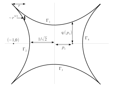
We describe ฮ“ฮ“\Gamma as a collection of four congruent curves. The part of ฮ“ฮ“\Gamma in the region {p2โ‰ฅ|p1|}subscript๐‘2subscript๐‘1\{p_{2}\geq|p_{1}|\} can be written as a graph

ฮ“1={(p1,ฯ†โ€‹(p1))}subscriptฮ“1subscript๐‘1๐œ‘subscript๐‘1\Gamma_{1}=\{(p_{1},\varphi(p_{1}))\}

for p1โˆˆ[โˆ’1,1]subscript๐‘111p_{1}\in[-1,1], where ฯ†๐œ‘\varphi is even, uniformly convex, tangent to p12=p22superscriptsubscript๐‘12superscriptsubscript๐‘22p_{1}^{2}=p_{2}^{2} at ยฑ1plus-or-minus1\pm 1, and separates from these lines like (dist)3/2superscriptdist32(\text{dist})^{3/2}. We will give a more precise description of ฯ†๐œ‘\varphi in Section 3.

The other pieces of ฮ“ฮ“\Gamma can be written

ฮ“2={โˆ’ฯ†โ€‹(p2),p2},ฮ“3={p1,โˆ’ฯ†โ€‹(p1)},ฮ“4={ฯ†โ€‹(p2),p2}formulae-sequencesubscriptฮ“2๐œ‘subscript๐‘2subscript๐‘2formulae-sequencesubscriptฮ“3subscript๐‘1๐œ‘subscript๐‘1subscriptฮ“4๐œ‘subscript๐‘2subscript๐‘2\Gamma_{2}=\{-\varphi(p_{2}),p_{2}\},\quad\Gamma_{3}=\{p_{1},-\varphi(p_{1})\},\quad\Gamma_{4}=\{\varphi(p_{2}),p_{2}\}

for piโˆˆ[โˆ’1,1]subscript๐‘๐‘–11p_{i}\in[-1,1], representing the left, bottom and right pieces of ฮ“ฮ“\Gamma (see figure 1).

Refer to caption
Figure 1. ฮ“ฮ“\Gamma consists of four identical curves separating from the lines p12=p22superscriptsubscript๐‘12superscriptsubscript๐‘22p_{1}^{2}=p_{2}^{2} like dist3/2.superscriptdist32\text{dist}^{3/2}.

Recall that u0=wโ€‹(x1,x22+x32)subscript๐‘ข0๐‘คsubscript๐‘ฅ1superscriptsubscript๐‘ฅ22superscriptsubscript๐‘ฅ32u_{0}=w\left(x_{1},\sqrt{x_{2}^{2}+x_{3}^{2}}\right). Then

ฮฉ=โˆ‡u0โ€‹(S2)ฮฉโˆ‡subscript๐‘ข0superscript๐‘†2\Omega=\nabla u_{0}(S^{2})

is the surface obtained by revolving ฮ“ฮ“\Gamma around the p1subscript๐‘1p_{1} axis. Let ฮฉRโŠ‚ฮฉsubscriptฮฉ๐‘…ฮฉ\Omega_{R}\subset\Omega be the surface obtained by revolving ฮ“1subscriptฮ“1\Gamma_{1} around the p1subscript๐‘1p_{1} axis.

In the statement below, ฮด๐›ฟ\delta and ฮณ๐›พ\gamma are small positive constants depending on ฯ†๐œ‘\varphi.

Proposition 2.4.

For any ฯต>0italic-ฯต0\epsilon>0 there exists a smooth function G๐บG defined in a neighborhood of ฮฉฮฉ\Omega such that

divโ€‹(โˆ‡Gโ€‹(โˆ‡u0))=0inB1โˆ–{0},divโˆ‡๐บโˆ‡subscript๐‘ข00insubscript๐ต10\text{div}(\nabla G(\nabla u_{0}))=0\quad\quad\mbox{in}\quad B_{1}\setminus\{0\},

and

  1. (1)

    If pโˆˆฮฉRโˆฉ{โˆ’1+ฮดโ‰คp1โ‰ค1โˆ’ฮด}๐‘subscriptฮฉ๐‘…1๐›ฟsubscript๐‘11๐›ฟp\in\Omega_{R}\cap\{-1+\delta\leq p_{1}\leq 1-\delta\} then SGโ€‹(p,q)โ‰ฅฮณโ€‹|pโˆ’q|2subscript๐‘†๐บ๐‘๐‘ž๐›พsuperscript๐‘๐‘ž2S_{G}(p,q)\geq\gamma|p-q|^{2} for all qโˆˆฮฉ๐‘žฮฉq\in\Omega,

  2. (2)

    SGโ€‹(p,q)โ‰ฅโˆ’ฯตโ€‹|pโˆ’q|2subscript๐‘†๐บ๐‘๐‘žitalic-ฯตsuperscript๐‘๐‘ž2S_{G}(p,q)\geq-\epsilon|p-q|^{2} otherwise for p,qโˆˆฮฉ๐‘๐‘žฮฉp,\,q\in\Omega.

We delay the proof of this proposition to Section 3, and use it now to prove Theorem 1.2.

2.3. Proof of Theorem 1.2

Recall that

u1โ€‹(x1,x2,x3)=u0โ€‹(x1/2,x2,x3),u2โ€‹(x1,x2,x3)=u1โ€‹(x3,x2,x1),formulae-sequencesuperscript๐‘ข1subscript๐‘ฅ1subscript๐‘ฅ2subscript๐‘ฅ3subscript๐‘ข0subscript๐‘ฅ12subscript๐‘ฅ2subscript๐‘ฅ3superscript๐‘ข2subscript๐‘ฅ1subscript๐‘ฅ2subscript๐‘ฅ3superscript๐‘ข1subscript๐‘ฅ3subscript๐‘ฅ2subscript๐‘ฅ1u^{1}(x_{1},x_{2},x_{3})=u_{0}(x_{1}/2,x_{2},x_{3}),\quad u^{2}(x_{1},x_{2},x_{3})=u^{1}(x_{3},x_{2},x_{1}),

and let

G1โ€‹(p1,p2,p3)=Gโ€‹(2โ€‹p1,p2,p3),G2โ€‹(p1,p2,p3)=G1โ€‹(p3,p2,p1).formulae-sequencesubscript๐บ1subscript๐‘1subscript๐‘2subscript๐‘3๐บ2subscript๐‘1subscript๐‘2subscript๐‘3subscript๐บ2subscript๐‘1subscript๐‘2subscript๐‘3subscript๐บ1subscript๐‘3subscript๐‘2subscript๐‘1G_{1}(p_{1},p_{2},p_{3})=G(2p_{1},p_{2},p_{3}),\quad G_{2}(p_{1},p_{2},p_{3})=G_{1}(p_{3},p_{2},p_{1}).

Then by Proposition 2.4 we have divโ€‹(โˆ‡Giโ€‹(โˆ‡ui))=0divโˆ‡subscript๐บ๐‘–โˆ‡superscript๐‘ข๐‘–0\text{div}(\nabla G_{i}(\nabla u^{i}))=0. Let

ฮฃ=Dโ€‹๐ฎโ€‹(B1).ฮฃ๐ท๐ฎsubscript๐ต1\Sigma=D{\bf u}(B_{1}).

Since D2โ€‹u1superscript๐ท2superscript๐‘ข1D^{2}u^{1} has rank 222 away from the cone

K1={x12โ‰ฅ4โ€‹(x22+x32)}subscript๐พ1superscriptsubscript๐‘ฅ124superscriptsubscript๐‘ฅ22superscriptsubscript๐‘ฅ32K_{1}=\left\{x_{1}^{2}\geq 4(x_{2}^{2}+x_{3}^{2})\right\}

and similarly D2โ€‹u2superscript๐ท2superscript๐‘ข2D^{2}u^{2} has rank 222 away from

K2={x32โ‰ฅ4โ€‹(x12+x22)},subscript๐พ2superscriptsubscript๐‘ฅ324superscriptsubscript๐‘ฅ12superscriptsubscript๐‘ฅ22K_{2}=\left\{x_{3}^{2}\geq 4(x_{1}^{2}+x_{2}^{2})\right\},

it is easy to see that ฮฃฮฃ\Sigma is a smooth embedded surface in โ„6superscriptโ„6\mathbb{R}^{6}.

Let

ฮฉi=โˆ‡uiโ€‹(B1โˆ’Ki).subscriptฮฉ๐‘–โˆ‡superscript๐‘ข๐‘–subscript๐ต1subscript๐พ๐‘–\Omega_{i}=\nabla u^{i}(B_{1}-K_{i}).

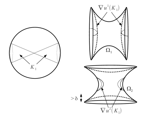
Note that ฮฉ1subscriptฮฉ1\Omega_{1} is just ฮฉRsubscriptฮฉ๐‘…\Omega_{R} squeezed by a factor of 1/2121/2 in the p1subscript๐‘1p_{1} direction. Let ฮฝisubscript๐œˆ๐‘–\nu_{i} be the outer normals to ฮฉisubscriptฮฉ๐‘–\Omega_{i}. Since uisuperscript๐‘ข๐‘–u^{i} are homogeneous degree one we have ฮฝiโ€‹(โˆ‡uiโ€‹(x))=xsubscript๐œˆ๐‘–โˆ‡superscript๐‘ข๐‘–๐‘ฅ๐‘ฅ\nu_{i}(\nabla u^{i}(x))=x on (B1โˆ’Ki)โˆฉS2subscript๐ต1subscript๐พ๐‘–superscript๐‘†2(B_{1}-K_{i})\cap S^{2}. Furthermore, the preimage xโˆˆS2๐‘ฅsuperscript๐‘†2x\in S^{2} of any point in ฮฃฮฃ\Sigma satisfies either |x1|โ‰ค|x3|subscript๐‘ฅ1subscript๐‘ฅ3|x_{1}|\leq|x_{3}| or vice versa. It follows from these observations that if (p1,p2)โˆˆฮฃsuperscript๐‘1superscript๐‘2ฮฃ(p^{1},p^{2})\in\Sigma then either

p1โˆˆฮฉ1โˆฉ{โˆ’ฮฒ/2โ‰คp11โ‰คฮฒ/2}โ€‹ย orย โ€‹p2โˆˆฮฉ2โˆฉ{โˆ’ฮฒ/2โ‰คp32โ‰คฮฒ/2}superscript๐‘1subscriptฮฉ1๐›ฝ2subscriptsuperscript๐‘11๐›ฝ2ย orย superscript๐‘2subscriptฮฉ2๐›ฝ2subscriptsuperscript๐‘23๐›ฝ2p^{1}\in\Omega_{1}\cap\{-\beta/2\leq p^{1}_{1}\leq\beta/2\}\text{ or }p^{2}\in\Omega_{2}\cap\{-\beta/2\leq p^{2}_{3}\leq\beta/2\}

with ฮฒ๐›ฝ\beta such that ฯ†โ€ฒโ€‹(ฮฒ)=1/2superscript๐œ‘โ€ฒ๐›ฝ12\varphi^{\prime}(\beta)=1/2, ฮฒ<1โˆ’ฮด๐›ฝ1๐›ฟ\beta<1-\delta (see figure 2). Assume p1superscript๐‘1p^{1} belongs to the set above.

Refer to caption
Figure 2. โˆ‡u1โˆ‡superscript๐‘ข1\nabla u^{1} maps the cone K1subscript๐พ1K_{1} to a region where G1subscript๐บ1G_{1} is slightly non-convex, but โˆ‡u2โˆ‡superscript๐‘ข2\nabla u^{2} maps it well inside ฮฉ2subscriptฮฉ2\Omega_{2} where G2subscript๐บ2G_{2} is uniformly convex.

Finally, let

F0โ€‹(p1,p2)=G1โ€‹(p1)+G2โ€‹(p2).subscript๐น0superscript๐‘1superscript๐‘2subscript๐บ1superscript๐‘1subscript๐บ2superscript๐‘2F_{0}(p^{1},p^{2})=G_{1}(p^{1})+G_{2}(p^{2}).

By rescaling Proposition 2.4 we have for (p1,p2),(q1,q2)โˆˆฮฃsuperscript๐‘1superscript๐‘2superscript๐‘ž1superscript๐‘ž2ฮฃ(p^{1},p^{2}),\,(q^{1},q^{2})\in\Sigma that

SF0โ€‹((p1,p2),(q1,q2))subscript๐‘†subscript๐น0superscript๐‘1superscript๐‘2superscript๐‘ž1superscript๐‘ž2\displaystyle S_{F_{0}}((p^{1},p^{2}),(q^{1},q^{2})) =SG1โ€‹(p1,q1)+SG2โ€‹(p2,q2)absentsubscript๐‘†subscript๐บ1superscript๐‘1superscript๐‘ž1subscript๐‘†subscript๐บ2superscript๐‘2superscript๐‘ž2\displaystyle=S_{G_{1}}(p^{1},q^{1})+S_{G_{2}}(p^{2},q^{2})
โ‰ฅฮณโ€‹|p1โˆ’q1|2โˆ’ฯตโ€‹|p2โˆ’q2|2.absent๐›พsuperscriptsuperscript๐‘1superscript๐‘ž12italic-ฯตsuperscriptsuperscript๐‘2superscript๐‘ž22\displaystyle\geq\gamma|p^{1}-q^{1}|^{2}-\epsilon|p^{2}-q^{2}|^{2}.

Let ฯ‰0โˆˆS2subscript๐œ”0superscript๐‘†2\omega_{0}\in S^{2} be a preimage of p1superscript๐‘1p^{1} under โˆ‡u1โˆ‡superscript๐‘ข1\nabla u^{1}. Then |โˆ‡u1โ€‹(ฯ‰)โˆ’โˆ‡u1โ€‹(ฯ‰0)|>cโ€‹|ฯ‰โˆ’ฯ‰0|โˆ‡superscript๐‘ข1๐œ”โˆ‡superscript๐‘ข1subscript๐œ”0๐‘๐œ”subscript๐œ”0|\nabla u^{1}(\omega)-\nabla u^{1}(\omega_{0})|>c|\omega-\omega_{0}| and |โˆ‡uiโ€‹(ฯ‰)โˆ’โˆ‡uiโ€‹(ฯ‰0)|<Cโ€‹|ฯ‰โˆ’ฯ‰0|โˆ‡superscript๐‘ข๐‘–๐œ”โˆ‡superscript๐‘ข๐‘–subscript๐œ”0๐ถ๐œ”subscript๐œ”0|\nabla u^{i}(\omega)-\nabla u^{i}(\omega_{0})|<C|\omega-\omega_{0}| for any ฯ‰โˆˆS2๐œ”superscript๐‘†2\omega\in S^{2}, so

|p2โˆ’q2|โ‰คCโ€‹|p1โˆ’q1|,superscript๐‘2superscript๐‘ž2๐ถsuperscript๐‘1superscript๐‘ž1|p^{2}-q^{2}|\leq C|p^{1}-q^{1}|,

giving quadratic separation. By Corollary 2.3 there is a smooth uniformly convex function F๐นF on โ„6superscriptโ„6\mathbb{R}^{6} so that F=F0๐นsubscript๐น0F=F_{0} and โˆ‡F=โˆ‡F0โˆ‡๐นโˆ‡subscript๐น0\nabla F=\nabla F_{0} on ฮฃฮฃ\Sigma, hence ๐ฎ๐ฎ\bf u satisfies the Euler-Lagrange system divโ€‹(โˆ‡Fโ€‹(Dโ€‹๐ฎ))=0divโˆ‡๐น๐ท๐ฎ0\text{div}(\nabla F(D{\bf u}))=0 in B1โˆ–{0}subscript๐ต10B_{1}\setminus\{0\}. Now it is straightforward to check that ๐ฎ๐ฎ\bf u is a weak solution of the system in the whole B1subscript๐ต1B_{1}. Indeed

โˆซB1โˆ‡Fโ€‹(Dโ€‹๐ฎ)โ‹…Dโ€‹ฯˆ=0,โˆ€ฯˆโˆˆC0โˆžโ€‹(B1),formulae-sequencesubscriptsubscript๐ต1โ‹…โˆ‡๐น๐ท๐ฎ๐ท๐œ“0for-all๐œ“superscriptsubscript๐ถ0subscript๐ต1\int_{B_{1}}\nabla F(D{\bf u})\cdot D\psi=0,\quad\quad\forall\psi\in C_{0}^{\infty}(B_{1}),

follows by integrating first by parts in B1โˆ–Bฯตsubscript๐ต1subscript๐ตitalic-ฯตB_{1}\setminus B_{\epsilon} and then letting ฯตโ†’0โ†’italic-ฯต0\epsilon\to 0.

3. Constructions

In this section we prove the key step, Proposition 2.4. Since ฮฉ=โˆ‡u0โ€‹(B1)ฮฉโˆ‡subscript๐‘ข0subscript๐ต1\Omega=\nabla u_{0}(B_{1}) is the surface obtained by revolving ฮ“ฮ“\Gamma around the p1subscript๐‘1p_{1} axis, we can reduce to a one-dimensional problem on ฮ“ฮ“\Gamma and then revolve the resulting picture around the p1subscript๐‘1p_{1} axis. Since all of our constructions will be on โ„2superscriptโ„2\mathbb{R}^{2} in this section we use coordinates (x,y)๐‘ฅ๐‘ฆ(x,y) rather than (p1,p2)subscript๐‘1subscript๐‘2(p_{1},p_{2}).

3.1. Setup

Define H๐ปH to be an even function in x๐‘ฅx and y๐‘ฆy which has the form

(3.1) Hโ€‹(x,y)=fโ€‹(x)+hโ€‹(x)โ€‹(|y|โˆ’ฯ†โ€‹(x)),๐ป๐‘ฅ๐‘ฆ๐‘“๐‘ฅโ„Ž๐‘ฅ๐‘ฆ๐œ‘๐‘ฅH(x,y)=f(x)+h(x)(|y|-\varphi(x)),

and is defined in a neighborhood of every point on ฮ“1โˆชฮ“3subscriptฮ“1subscriptฮ“3\Gamma_{1}\cup\Gamma_{3}, for some smooth functions f๐‘“f and hโ„Žh on [โˆ’1,1]11[-1,1]. In our construction hโ„Žh will be identically zero and f๐‘“f linear near x=ยฑ1๐‘ฅplus-or-minus1x=\pm 1, so H๐ปH is linear in a neighborhood of the cusps of ฮ“ฮ“\Gamma. Notice that we can extend H๐ปH to be a linear function (depending only on x๐‘ฅx) in a whole neighborhood of ฮ“2subscriptฮ“2\Gamma_{2} and similarly on ฮ“4subscriptฮ“4\Gamma_{4}. Then H๐ปH is defined and smooth in a neighborhood of ฮ“ฮ“\Gamma.

3.2. Inequalities for ฯ†๐œ‘\varphi

We now record some useful properties of ฮ“ฮ“\Gamma. For proofs see Section 4. The first estimate gives an expansion for ฯ†๐œ‘\varphi near x=โˆ’1๐‘ฅ1x=-1.

Proposition 3.1.

The function ฯ†๐œ‘\varphi is even, uniformly convex, and tangent to y=|x|๐‘ฆ๐‘ฅy=|x| at x=ยฑ1๐‘ฅplus-or-minus1x=\pm 1. Furthermore, ฯ†โ€ฒโ€ฒsuperscript๐œ‘โ€ฒโ€ฒ\varphi^{\prime\prime} is decreasing near x=โˆ’1๐‘ฅ1x=-1 and we have the expansion

(3.2) ฯ†โ€ฒโ€ฒโ€‹(โˆ’1+ฯต)=23โ€‹ฯตโˆ’1/2+Oโ€‹(1).superscript๐œ‘โ€ฒโ€ฒ1italic-ฯต23superscriptitalic-ฯต12๐‘‚1\varphi^{\prime\prime}(-1+\epsilon)=\sqrt{\frac{2}{3}}\epsilon^{-1/2}+O(1).

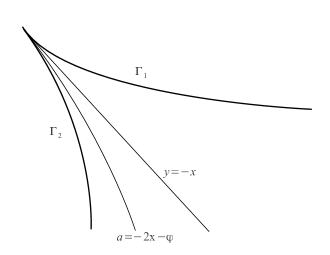
The second estimate says that the vertical reflection of ฯ†๐œ‘\varphi over its tangent y=โˆ’x๐‘ฆ๐‘ฅy=-x lies above and separates from ฮ“2subscriptฮ“2\Gamma_{2} (see figure 3). It follows easily from the uniform convexity of ฯ†๐œ‘\varphi.

Proposition 3.2.

The function aโ€‹(x)=โˆ’2โ€‹xโˆ’ฯ†๐‘Ž๐‘ฅ2๐‘ฅ๐œ‘a(x)=-2x-\varphi is uniformly concave, tangent to ฮ“2subscriptฮ“2\Gamma_{2} at x=โˆ’1๐‘ฅ1x=-1, and lies strictly above ฮ“2subscriptฮ“2\Gamma_{2} for x>โˆ’1๐‘ฅ1x>-1.

Refer to caption
Figure 3. The graph a=โˆ’2โ€‹xโˆ’ฯ†๐‘Ž2๐‘ฅ๐œ‘a=-2x-\varphi lies strictly above ฮ“2subscriptฮ“2\Gamma_{2}.

3.3. Euler-Lagrange Equation

Let

Gโ€‹(p1,p2,p3)=Hโ€‹(p1,p22+p32).๐บsubscript๐‘1subscript๐‘2subscript๐‘3๐ปsubscript๐‘1superscriptsubscript๐‘22superscriptsubscript๐‘32G(p_{1},p_{2},p_{3})=H\left(p_{1},\sqrt{p_{2}^{2}+p_{3}^{2}}\right).

The condition that u0subscript๐‘ข0u_{0} solves the Euler-Lagrange equation divโ€‹(โˆ‡Gโ€‹(โˆ‡u0))=0divโˆ‡๐บโˆ‡subscript๐‘ข00\text{div}(\nabla G(\nabla u_{0}))=0 is equivalent to

(3.3) hโ€‹(x)=fโ€ฒโ€ฒโ€‹(x)2โ€‹ฯ†โ€ฒโ€ฒโ€‹(x).โ„Ž๐‘ฅsuperscript๐‘“โ€ฒโ€ฒ๐‘ฅ2superscript๐œ‘โ€ฒโ€ฒ๐‘ฅh(x)=\frac{f^{\prime\prime}(x)}{2\varphi^{\prime\prime}(x)}.

Indeed, since G๐บG is linear near the surfaces obtained by revolving ฮ“2subscriptฮ“2\Gamma_{2} and ฮ“4subscriptฮ“4\Gamma_{4}, we just need to verify the Euler-Lagrange equation where โˆ‡u0โˆ‡subscript๐‘ข0\nabla u_{0} is on the surface ฮฉRsubscriptฮฉ๐‘…\Omega_{R} obtained by revolving ฮ“1subscriptฮ“1\Gamma_{1}. By passing a derivative the Euler-Lagrange equation divโ€‹(โˆ‡Gโ€‹(โˆ‡u0))divโˆ‡๐บโˆ‡subscript๐‘ข0\text{div}(\nabla G(\nabla u_{0})) is equivalent to

trโ€‹(D2โ€‹Gโ€‹(โˆ‡u0)โ‹…D2โ€‹u0)=0.trโ‹…superscript๐ท2๐บโˆ‡subscript๐‘ข0superscript๐ท2subscript๐‘ข00\text{tr}\left(D^{2}G(\nabla u_{0})\cdot D^{2}u_{0}\right)=0.

Let ฮฉRsubscriptฮฉ๐‘…\Omega_{R} have outer normal ฮฝ๐œˆ\nu and second fundamental form Iโ€‹I๐ผ๐ผII. Since u0subscript๐‘ข0u_{0} is homogeneous degree one we have ฮฝโ€‹(โˆ‡u0โ€‹(x))=x๐œˆโˆ‡subscript๐‘ข0๐‘ฅ๐‘ฅ\nu(\nabla u_{0}(x))=x on S2superscript๐‘†2S^{2}. Let T๐‘‡T be a frame tangent to S2superscript๐‘†2S^{2} at x๐‘ฅx, and differentiate to obtain DT2โ€‹u0โ€‹(x)=Iโ€‹Iโˆ’1โ€‹(โˆ‡u0โ€‹(x)).superscriptsubscript๐ท๐‘‡2subscript๐‘ข0๐‘ฅ๐ผsuperscript๐ผ1โˆ‡subscript๐‘ข0๐‘ฅD_{T}^{2}u_{0}(x)=II^{-1}(\nabla u_{0}(x)). In coordinates tangent to ฮฉRsubscriptฮฉ๐‘…\Omega_{R} at p=(p1,ฯ†โ€‹(p1),0)๐‘subscript๐‘1๐œ‘subscript๐‘10p=(p_{1},\varphi(p_{1}),0) one computes

Iโ€‹I=11+ฯ†โ€ฒโฃ2โ€‹(ฯ†โ€ฒโ€ฒ1+ฯ†โ€ฒโฃ200โˆ’1ฯ†),D2โ€‹G=(fโ€ฒโ€ฒโˆ’hโ€‹ฯ†โ€ฒโ€ฒ1+ฯ†โ€ฒโฃ200hฯ†)formulae-sequence๐ผ๐ผ11superscript๐œ‘โ€ฒ2superscript๐œ‘โ€ฒโ€ฒ1superscript๐œ‘โ€ฒ2001๐œ‘superscript๐ท2๐บsuperscript๐‘“โ€ฒโ€ฒโ„Žsuperscript๐œ‘โ€ฒโ€ฒ1superscript๐œ‘โ€ฒ200โ„Ž๐œ‘II=\frac{1}{\sqrt{1+\varphi^{\prime 2}}}\left(\begin{array}[]{cc}\frac{\varphi^{\prime\prime}}{1+\varphi^{\prime 2}}&0\\ 0&-\frac{1}{\varphi}\end{array}\right),\quad D^{2}G=\left(\begin{array}[]{cc}\frac{f^{\prime\prime}-h\varphi^{\prime\prime}}{1+\varphi^{\prime 2}}&0\\ 0&\frac{h}{\varphi}\end{array}\right)

and the Euler-Lagrange formula follows.

Remark 3.3.

For a fast way to compute D2โ€‹Gsuperscript๐ท2๐บD^{2}G in tangential coordinates, differentiate the equation Gโ€‹(p1,ฯ†โ€‹(p1),0)=fโ€‹(p1)๐บsubscript๐‘1๐œ‘subscript๐‘10๐‘“subscript๐‘1G(p_{1},\varphi(p_{1}),0)=f(p_{1}):

โˆ‡Gโ‹…(1,ฯ†โ€ฒ)=fโ€ฒ,(1,ฯ†โ€ฒ)Tโ‹…D2โ€‹Gโ‹…(1,ฯ†โ€ฒ)+hโ€‹ฯ†โ€ฒโ€ฒ=fโ€ฒโ€ฒ.formulae-sequenceโ‹…โˆ‡๐บ1superscript๐œ‘โ€ฒsuperscript๐‘“โ€ฒโ‹…โ‹…superscript1superscript๐œ‘โ€ฒ๐‘‡superscript๐ท2๐บ1superscript๐œ‘โ€ฒโ„Žsuperscript๐œ‘โ€ฒโ€ฒsuperscript๐‘“โ€ฒโ€ฒ\nabla G\cdot(1,\varphi^{\prime})=f^{\prime},\quad(1,\varphi^{\prime})^{T}\cdot D^{2}G\cdot(1,\varphi^{\prime})+h\varphi^{\prime\prime}=f^{\prime\prime}.

The other eigenvalue comes from the rotational symmetry of G๐บG around the p1subscript๐‘1p_{1} axis.

Remark 3.4.

If we do the computation in โ„nsuperscriptโ„๐‘›\mathbb{R}^{n} we have nโˆ’1๐‘›1n-1 rotational principal curvatures and derivatives, giving the Euler-Lagrange equation h=fโ€ฒโ€ฒ(nโˆ’1)โ€‹ฯ†โ€ฒโ€ฒโ„Žsuperscript๐‘“โ€ฒโ€ฒ๐‘›1superscript๐œ‘โ€ฒโ€ฒh=\frac{f^{\prime\prime}}{(n-1)\varphi^{\prime\prime}}.

3.4. Convexity Conditions

Since most of our analysis is near a cusp, it is convenient to shift the picture by the vector (1,โˆ’1)11(1,-1) so that ฯ†,f๐œ‘๐‘“\varphi,\,f are defined on [0,2]02[0,2] and ฯ†๐œ‘\varphi is tangent to y=โˆ’x๐‘ฆ๐‘ฅy=-x at zero. We assume this for the remainder of the section.

We examine convexity conditions between two points on ฮ“1subscriptฮ“1\Gamma_{1}. Let p=(x0,ฯ†โ€‹(x0))๐‘subscript๐‘ฅ0๐œ‘subscript๐‘ฅ0p=(x_{0},\varphi(x_{0})) and q=(x,ฯ†โ€‹(x))๐‘ž๐‘ฅ๐œ‘๐‘ฅq=(x,\varphi(x)). We first write the equation for the tangent plane Lpsubscript๐ฟ๐‘L_{p} to H๐ปH at p=(x0,ฯ†โ€‹(x0))๐‘subscript๐‘ฅ0๐œ‘subscript๐‘ฅ0p=(x_{0},\varphi(x_{0})):

Lpโ€‹(x,y)=fโ€‹(x0)+fโ€ฒโ€‹(x0)โ€‹(xโˆ’x0)+hโ€‹(x0)โ€‹[yโˆ’(ฯ†โ€‹(x0)+ฯ†โ€ฒโ€‹(x0)โ€‹(xโˆ’x0))].subscript๐ฟ๐‘๐‘ฅ๐‘ฆ๐‘“subscript๐‘ฅ0superscript๐‘“โ€ฒsubscript๐‘ฅ0๐‘ฅsubscript๐‘ฅ0โ„Žsubscript๐‘ฅ0delimited-[]๐‘ฆ๐œ‘subscript๐‘ฅ0superscript๐œ‘โ€ฒsubscript๐‘ฅ0๐‘ฅsubscript๐‘ฅ0L_{p}(x,y)=f(x_{0})+f^{\prime}(x_{0})(x-x_{0})+h(x_{0})\left[y-(\varphi(x_{0})+\varphi^{\prime}(x_{0})(x-x_{0}))\right].

Applying the Euler-Lagrange equation (3.3) we obtain

(3.4) Lp=fโ€‹(x0)+fโ€ฒโ€‹(x0)โ€‹(xโˆ’x0)โˆ’fโ€ฒโ€ฒโ€‹(x0)2โ€‹ฯ†โ€ฒโ€ฒโ€‹(x0)โ€‹[yโˆ’(ฯ†โ€‹(x0)+ฯ†โ€ฒโ€‹(x0)โ€‹(xโˆ’x0))].subscript๐ฟ๐‘๐‘“subscript๐‘ฅ0superscript๐‘“โ€ฒsubscript๐‘ฅ0๐‘ฅsubscript๐‘ฅ0superscript๐‘“โ€ฒโ€ฒsubscript๐‘ฅ02superscript๐œ‘โ€ฒโ€ฒsubscript๐‘ฅ0delimited-[]๐‘ฆ๐œ‘subscript๐‘ฅ0superscript๐œ‘โ€ฒsubscript๐‘ฅ0๐‘ฅsubscript๐‘ฅ0L_{p}=f(x_{0})+f^{\prime}(x_{0})(x-x_{0})-\frac{f^{\prime\prime}(x_{0})}{2\varphi^{\prime\prime}(x_{0})}\left[y-(\varphi(x_{0})+\varphi^{\prime}(x_{0})(x-x_{0}))\right].

By definition,

SHโ€‹(p,q)=fโ€‹(x)โˆ’Lpโ€‹(x,ฯ†โ€‹(x)).subscript๐‘†๐ป๐‘๐‘ž๐‘“๐‘ฅsubscript๐ฟ๐‘๐‘ฅ๐œ‘๐‘ฅS_{H}(p,q)=f(x)-L_{p}(x,\varphi(x)).

Using equation (3.4) we obtain

(3.5) SHโ€‹(p,q)=โˆซx0xfโ€ฒโ€ฒโ€‹(t)โ€‹(xโˆ’t)โ€‹๐‘‘tโˆ’fโ€ฒโ€ฒโ€‹(x0)2โ€‹ฯ†โ€ฒโ€ฒโ€‹(x0)โ€‹โˆซx0xฯ†โ€ฒโ€ฒโ€‹(t)โ€‹(xโˆ’t)โ€‹๐‘‘t.subscript๐‘†๐ป๐‘๐‘žsuperscriptsubscriptsubscript๐‘ฅ0๐‘ฅsuperscript๐‘“โ€ฒโ€ฒ๐‘ก๐‘ฅ๐‘กdifferential-d๐‘กsuperscript๐‘“โ€ฒโ€ฒsubscript๐‘ฅ02superscript๐œ‘โ€ฒโ€ฒsubscript๐‘ฅ0superscriptsubscriptsubscript๐‘ฅ0๐‘ฅsuperscript๐œ‘โ€ฒโ€ฒ๐‘ก๐‘ฅ๐‘กdifferential-d๐‘กS_{H}(p,q)=\int_{x_{0}}^{x}f^{\prime\prime}(t)(x-t)\,dt-\frac{f^{\prime\prime}(x_{0})}{2\varphi^{\prime\prime}(x_{0})}\int_{x_{0}}^{x}\varphi^{\prime\prime}(t)(x-t)\,dt.
Definition 3.5.

For a nonnegative function g:โ„โ†’โ„:๐‘”โ†’โ„โ„g:\mathbb{R}\rightarrow\mathbb{R} define the weighted average

sgโ€‹(x0,x)=โˆซx0xgโ€‹(t)โ€‹(xโˆ’t)โ€‹๐‘‘tgโ€‹(x0)โ€‹(xโˆ’x0)2.subscript๐‘ ๐‘”subscript๐‘ฅ0๐‘ฅsuperscriptsubscriptsubscript๐‘ฅ0๐‘ฅ๐‘”๐‘ก๐‘ฅ๐‘กdifferential-d๐‘ก๐‘”subscript๐‘ฅ0superscript๐‘ฅsubscript๐‘ฅ02s_{g}(x_{0},x)=\frac{\int_{x_{0}}^{x}g(t)(x-t)\,dt}{g(x_{0})(x-x_{0})^{2}}.

With this definition we have

(3.6) SHโ€‹(p,q)=fโ€ฒโ€ฒโ€‹(x0)โ€‹(sfโ€ฒโ€ฒโ€‹(x0,x)โˆ’12โ€‹sฯ†โ€ฒโ€ฒโ€‹(x0,x))โ€‹(xโˆ’x0)2,subscript๐‘†๐ป๐‘๐‘žsuperscript๐‘“โ€ฒโ€ฒsubscript๐‘ฅ0subscript๐‘ superscript๐‘“โ€ฒโ€ฒsubscript๐‘ฅ0๐‘ฅ12subscript๐‘ superscript๐œ‘โ€ฒโ€ฒsubscript๐‘ฅ0๐‘ฅsuperscript๐‘ฅsubscript๐‘ฅ02S_{H}(p,q)=f^{\prime\prime}(x_{0})\left(s_{f^{\prime\prime}}(x_{0},x)-\frac{1}{2}s_{\varphi^{\prime\prime}}(x_{0},x)\right)(x-x_{0})^{2},

thus, the first qualitative convexity condition is

(3.7) sfโ€ฒโ€ฒโ€‹(x0,x)โ‰ฅ12โ€‹sฯ†โ€ฒโ€ฒโ€‹(x0,x).subscript๐‘ superscript๐‘“โ€ฒโ€ฒsubscript๐‘ฅ0๐‘ฅ12subscript๐‘ superscript๐œ‘โ€ฒโ€ฒsubscript๐‘ฅ0๐‘ฅs_{f^{\prime\prime}}(x_{0},x)\geq\frac{1}{2}s_{\varphi^{\prime\prime}}(x_{0},x).
Remark 3.6.

Notice that

limxโ†’x0sgโ€‹(x0,x)=12.subscriptโ†’๐‘ฅsubscript๐‘ฅ0subscript๐‘ ๐‘”subscript๐‘ฅ0๐‘ฅ12\lim_{x\to x_{0}}s_{g}(x_{0},x)=\frac{1}{2}.

It is easy to check that if g๐‘”g is increasing (decreasing) then sgโ€‹(x0,x)subscript๐‘ ๐‘”subscript๐‘ฅ0๐‘ฅs_{g}(x_{0},x) is increasing (decreasing) with x๐‘ฅx. With this observation one verifies that condition (3.7) holds for x0,xsubscript๐‘ฅ0๐‘ฅx_{0},\,x near 00 if fโ€ฒโ€ฒโ€‹(x)=Cโ€‹x1โˆ’ฮฑsuperscript๐‘“โ€ฒโ€ฒ๐‘ฅ๐ถsuperscript๐‘ฅ1๐›ผf^{\prime\prime}(x)=Cx^{1-\alpha} for any ฮฑโˆˆ(0,1)๐›ผ01\alpha\in(0,1). Indeed, since fโ€ฒโ€ฒsuperscript๐‘“โ€ฒโ€ฒf^{\prime\prime} is increasing and ฯ†โ€ฒโ€ฒsuperscript๐œ‘โ€ฒโ€ฒ\varphi^{\prime\prime} is decreasing one only needs to check the condition at x=0๐‘ฅ0x=0, where one computes sfโ€ฒโ€ฒโ€‹(x0,0)=13โˆ’ฮฑsubscript๐‘ superscript๐‘“โ€ฒโ€ฒsubscript๐‘ฅ0013๐›ผs_{f^{\prime\prime}}(x_{0},0)=\frac{1}{3-\alpha} and 12โ€‹sฯ†โ€ฒโ€ฒโ€‹(x0,0)=13+Oโ€‹(x0)12subscript๐‘ superscript๐œ‘โ€ฒโ€ฒsubscript๐‘ฅ0013๐‘‚subscript๐‘ฅ0\frac{1}{2}s_{\varphi^{\prime\prime}}(x_{0},0)=\frac{1}{3}+O(\sqrt{x_{0}}) which follows by Proposition 3.1.

We now examine convexity conditions between pโˆˆฮ“1๐‘subscriptฮ“1p\in\Gamma_{1} and qโˆˆฮ“2๐‘žsubscriptฮ“2q\in\Gamma_{2}.

Let p=(x0,ฯ†โ€‹(x0))๐‘subscript๐‘ฅ0๐œ‘subscript๐‘ฅ0p=(x_{0},\varphi(x_{0})). In our construction we will have hโ‰ฅ0โ„Ž0h\geq 0, and since H๐ปH is linear near ฮ“2subscriptฮ“2\Gamma_{2}, we see that SHโ€‹(p,q)โ‰ฅ0subscript๐‘†๐ป๐‘๐‘ž0S_{H}(p,q)\geq 0 if the intersection line of tangent planes to H๐ปH at p๐‘p and at 00 lies above the line y=โˆ’x๐‘ฆ๐‘ฅy=-x on [0,2]02[0,2]. Using equation (3.4) we compute the formula for the intersection line:

(3.8) y=ฯ†โ€‹(x0)โˆ’2โ€‹ฯ†โ€ฒโ€ฒโ€‹(x0)fโ€ฒโ€ฒโ€‹(x0)โ€‹โˆซ0x0fโ€ฒโ€ฒโ€‹(t)โ€‹(x0โˆ’t)โ€‹๐‘‘t+(ฯ†โ€ฒโ€‹(x0)โˆ’2โ€‹ฯ†โ€ฒโ€ฒโ€‹(x0)fโ€ฒโ€ฒโ€‹(x0)โ€‹โˆซ0x0fโ€ฒโ€ฒโ€‹(t)โ€‹๐‘‘t)โ‹…(xโˆ’x0).๐‘ฆ๐œ‘subscript๐‘ฅ02superscript๐œ‘โ€ฒโ€ฒsubscript๐‘ฅ0superscript๐‘“โ€ฒโ€ฒsubscript๐‘ฅ0superscriptsubscript0subscript๐‘ฅ0superscript๐‘“โ€ฒโ€ฒ๐‘กsubscript๐‘ฅ0๐‘กdifferential-d๐‘กโ‹…superscript๐œ‘โ€ฒsubscript๐‘ฅ02superscript๐œ‘โ€ฒโ€ฒsubscript๐‘ฅ0superscript๐‘“โ€ฒโ€ฒsubscript๐‘ฅ0superscriptsubscript0subscript๐‘ฅ0superscript๐‘“โ€ฒโ€ฒ๐‘กdifferential-d๐‘ก๐‘ฅsubscript๐‘ฅ0\begin{split}y=\varphi(x_{0})-\frac{2\varphi^{\prime\prime}(x_{0})}{f^{\prime\prime}(x_{0})}\int_{0}^{x_{0}}f^{\prime\prime}(t)(x_{0}-t)\,dt\\ +\left(\varphi^{\prime}(x_{0})-\frac{2\varphi^{\prime\prime}(x_{0})}{f^{\prime\prime}(x_{0})}\int_{0}^{x_{0}}f^{\prime\prime}(t)\,dt\right)\cdot(x-x_{0}).\end{split}

If condition (3.7) holds at x=0๐‘ฅ0x=0, it means that the origin lies below the intersection line, thus SHโ€‹(p,q)โ‰ฅ0subscript๐‘†๐ป๐‘๐‘ž0S_{H}(p,q)\geq 0 for all qโˆˆฮ“2๐‘žsubscriptฮ“2q\in\Gamma_{2} provided that the slope of the intersection line above is larger than โˆ’11-1:

ฯ†โ€ฒโ€‹(x0)โˆ’2โ€‹ฯ†โ€ฒโ€ฒโ€‹(x0)fโ€ฒโ€ฒโ€‹(x0)โ€‹โˆซ0x0fโ€ฒโ€ฒโ€‹(t)โ€‹๐‘‘tโ‰ฅโˆ’1=ฯ†โ€ฒโ€‹(0).superscript๐œ‘โ€ฒsubscript๐‘ฅ02superscript๐œ‘โ€ฒโ€ฒsubscript๐‘ฅ0superscript๐‘“โ€ฒโ€ฒsubscript๐‘ฅ0superscriptsubscript0subscript๐‘ฅ0superscript๐‘“โ€ฒโ€ฒ๐‘กdifferential-d๐‘ก1superscript๐œ‘โ€ฒ0\varphi^{\prime}(x_{0})-\frac{2\varphi^{\prime\prime}(x_{0})}{f^{\prime\prime}(x_{0})}\int_{0}^{x_{0}}f^{\prime\prime}(t)\,dt\geq-1=\varphi^{\prime}(0).
Definition 3.7.

For a nonnegative function g:โ„โ†’โ„:๐‘”โ†’โ„โ„g:\mathbb{R}\rightarrow\mathbb{R} define

dgโ€‹(x)=โˆซ0xgโ€‹(t)โ€‹๐‘‘txโ€‹gโ€‹(x).subscript๐‘‘๐‘”๐‘ฅsuperscriptsubscript0๐‘ฅ๐‘”๐‘กdifferential-d๐‘ก๐‘ฅ๐‘”๐‘ฅd_{g}(x)=\frac{\int_{0}^{x}g(t)\,dt}{xg(x)}.

With this definition the slope condition above can be written as

(3.9) dfโ€ฒโ€ฒโ€‹(x)โ‰ค12โ€‹dฯ†โ€ฒโ€ฒโ€‹(x).subscript๐‘‘superscript๐‘“โ€ฒโ€ฒ๐‘ฅ12subscript๐‘‘superscript๐œ‘โ€ฒโ€ฒ๐‘ฅd_{f^{\prime\prime}}(x)\leq\frac{1}{2}d_{\varphi^{\prime\prime}}(x).
Remark 3.8.

Near x=0๐‘ฅ0x=0 one computes 12โ€‹dฯ†โ€ฒโ€ฒโ€‹(x)=1+Oโ€‹(x)12subscript๐‘‘superscript๐œ‘โ€ฒโ€ฒ๐‘ฅ1๐‘‚๐‘ฅ\frac{1}{2}d_{\varphi^{\prime\prime}}(x)=1+O(\sqrt{x}). Thus, if fโ€ฒโ€ฒโ€‹(x)=Cโ€‹x1โˆ’ฮฑsuperscript๐‘“โ€ฒโ€ฒ๐‘ฅ๐ถsuperscript๐‘ฅ1๐›ผf^{\prime\prime}(x)=Cx^{1-\alpha} near x=0๐‘ฅ0x=0 then (3.9) holds. However, away from a small neighborhood of 00, condition (3.9) will not hold in our construction. We will use formula (3.4) more carefully, combined with Proposition 3.2, to deal with these cases.

Remark 3.9.

Conditions (3.7) and (3.9) are independent of the linear part of f๐‘“f. Thus, when checking convexity conditions we only need to use the properties of fโ€ฒโ€ฒsuperscript๐‘“โ€ฒโ€ฒf^{\prime\prime}.

3.5. Preliminary Construction

As a stepping stone to proving Proposition 2.4 we construct first a C1,ฮฑsuperscript๐ถ1๐›ผC^{1,\alpha} function H0subscript๐ป0H_{0} near ฮ“ฮ“\Gamma, that is globally convex. We will use this construction to prove Theorem 1.1 in Section 4. The function HโˆˆCโˆž๐ปsuperscript๐ถH\in C^{\infty} is obtained by perturbing H0subscript๐ป0H_{0}. Below we define

G0โ€‹(p1,p2,p3)=H0โ€‹(p1,p22+p33).subscript๐บ0subscript๐‘1subscript๐‘2subscript๐‘3subscript๐ป0subscript๐‘1superscriptsubscript๐‘22superscriptsubscript๐‘33G_{0}(p_{1},p_{2},p_{3})=H_{0}\left(p_{1},\sqrt{p_{2}^{2}+p_{3}^{3}}\right).

Recall in the constructions below that we have shifted the picture by (1,โˆ’1)11(1,-1).

Proposition 3.10.

For any ฮฑโˆˆ(0,1)๐›ผ01\alpha\in(0,1) there exist a function H0subscript๐ป0H_{0} near ฮ“ฮ“\Gamma such that

  1. (1)

    H0subscript๐ป0H_{0} is a linear function depending only on x๐‘ฅx on ฮ“2subscriptฮ“2\Gamma_{2}, and similarly on ฮ“4subscriptฮ“4\Gamma_{4}.

  2. (2)

    H0subscript๐ป0H_{0} is pointwise C1,1โˆ’ฮฑsuperscript๐ถ11๐›ผC^{1,1-\alpha} on the cusps of ฮ“ฮ“\Gamma and smooth otherwise,

  3. (3)

    divโ€‹(โˆ‡G0โ€‹(โˆ‡u0))=0divโˆ‡subscript๐บ0โˆ‡subscript๐‘ข00\text{div}(\nabla G_{0}(\nabla u_{0}))=0 away from the cone {x12=x22+x32},superscriptsubscript๐‘ฅ12superscriptsubscript๐‘ฅ22superscriptsubscript๐‘ฅ32\{x_{1}^{2}=x_{2}^{2}+x_{3}^{2}\},

  4. (4)

    SH0โ€‹(p,q)โ‰ฅ0subscript๐‘†subscript๐ป0๐‘๐‘ž0S_{H_{0}}(p,q)\geq 0 for all p,qโˆˆฮ“๐‘๐‘žฮ“p,\,q\in\Gamma,

  5. (5)

    If p=(x,ฯ†โ€‹(x))๐‘๐‘ฅ๐œ‘๐‘ฅp=(x,\varphi(x)) then SH0โ€‹(p,q)โ‰ฅฮทโ€‹(x)โ€‹|pโˆ’q|2subscript๐‘†subscript๐ป0๐‘๐‘ž๐œ‚๐‘ฅsuperscript๐‘๐‘ž2S_{H_{0}}(p,q)\geq\eta(x)|p-q|^{2} for all qโˆˆฮ“๐‘žฮ“q\in\Gamma, where ฮท๐œ‚\eta is some continuous function on [0,2]02[0,2] with ฮท>0๐œ‚0\eta>0 on (0,2)02(0,2) and ฮทโ€‹(0)=ฮทโ€‹(2)=0๐œ‚0๐œ‚20\eta(0)=\eta(2)=0.

We will define f0subscript๐‘“0f_{0} by f0โ€‹(0)=f0โ€ฒโ€‹(0)=0subscript๐‘“00superscriptsubscript๐‘“0โ€ฒ00f_{0}(0)=f_{0}^{\prime}(0)=0 and prescribe f0โ€ฒโ€ฒsuperscriptsubscript๐‘“0โ€ฒโ€ฒf_{0}^{\prime\prime}, and then let H0subscript๐ป0H_{0} be the function determined by f0subscript๐‘“0f_{0} through the Euler-Lagrange relation (3.3). It is easy to check that condition (3.7) holds if we take f0โ€ฒโ€ฒ=ฯ†โ€ฒโ€ฒsuperscriptsubscript๐‘“0โ€ฒโ€ฒsuperscript๐œ‘โ€ฒโ€ฒf_{0}^{\prime\prime}=\varphi^{\prime\prime}. However, we want h0=f0โ€ฒโ€ฒ/(2โ€‹ฯ†โ€ฒโ€ฒ)subscriptโ„Ž0superscriptsubscript๐‘“0โ€ฒโ€ฒ2superscript๐œ‘โ€ฒโ€ฒh_{0}=f_{0}^{\prime\prime}/(2\varphi^{\prime\prime}) to go to zero at the endpoints so that H0subscript๐ป0H_{0} is linear on ฮ“2subscriptฮ“2\Gamma_{2} and ฮ“4subscriptฮ“4\Gamma_{4}.
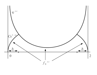
Motivated by the above and Remarks 3.6 and 3.8, define

f0โ€ฒโ€ฒโ€‹(x)={ฮดฮฑโˆ’1โ€‹ฯ†โ€ฒโ€ฒโ€‹(ฮด)โ€‹x1โˆ’ฮฑ,0โ‰คxโ‰คฮดฯ†โ€ฒโ€ฒโ€‹(x),ฮดโ‰คxโ‰ค1f0โ€ฒโ€ฒโ€‹(2โˆ’x),1โ‰คxโ‰ค2superscriptsubscript๐‘“0โ€ฒโ€ฒ๐‘ฅcasessuperscript๐›ฟ๐›ผ1superscript๐œ‘โ€ฒโ€ฒ๐›ฟsuperscript๐‘ฅ1๐›ผ0๐‘ฅ๐›ฟotherwisesuperscript๐œ‘โ€ฒโ€ฒ๐‘ฅ๐›ฟ๐‘ฅ1otherwisesuperscriptsubscript๐‘“0โ€ฒโ€ฒ2๐‘ฅ1๐‘ฅ2otherwisef_{0}^{\prime\prime}(x)=\begin{cases}\delta^{\alpha-1}\varphi^{\prime\prime}(\delta)x^{1-\alpha},\quad 0\leq x\leq\delta\\ \varphi^{\prime\prime}(x),\quad\delta\leq x\leq 1\\ f_{0}^{\prime\prime}(2-x),\quad 1\leq x\leq 2\end{cases}

(See figure 4). Assume ฮด๐›ฟ\delta is tiny so that ฯ†โ€ฒโ€ฒsuperscript๐œ‘โ€ฒโ€ฒ\varphi^{\prime\prime} is well approximated by its expansion (3.2). Let H0subscript๐ป0H_{0} be the function as in (3.1) determined by f0subscript๐‘“0f_{0} through the Euler-Lagrange relation (3.3).
Refer to caption
Figure 4. f0โ€ฒโ€ฒsuperscriptsubscript๐‘“0โ€ฒโ€ฒf_{0}^{\prime\prime} agrees with ฯ†โ€ฒโ€ฒsuperscript๐œ‘โ€ฒโ€ฒ\varphi^{\prime\prime} on [ฮด,2โˆ’ฮด]๐›ฟ2๐›ฟ[\delta,2-\delta], behaves like x1โˆ’ฮฑsuperscript๐‘ฅ1๐›ผx^{1-\alpha} near zero, and is symmetric around x=1๐‘ฅ1x=1.
Proof of proposition 3.10.

The first three items are clear by construction so we check the convexity conditions. By symmetry we only need to consider pโˆˆฮ“1โˆชฮ“2๐‘subscriptฮ“1subscriptฮ“2p\in\Gamma_{1}\cup\Gamma_{2}.

If pโˆˆฮ“2๐‘subscriptฮ“2p\in\Gamma_{2} the positive separation is a consequence of H0โ‰ฅ0subscript๐ป00H_{0}\geq 0. This follows from the definition of H0subscript๐ป0H_{0} on ฮ“1โˆชฮ“3subscriptฮ“1subscriptฮ“3\Gamma_{1}\cup\Gamma_{3}. Also, by symmetry, the linear function on ฮ“4subscriptฮ“4\Gamma_{4} intersects the linear function on ฮ“2subscriptฮ“2\Gamma_{2} on the vertical line {x=1}๐‘ฅ1\{x=1\}, and since ฮ“4โŠ‚{x>1}subscriptฮ“4๐‘ฅ1\Gamma_{4}\subset\{x>1\} we obtain H0โ‰ฅ0subscript๐ป00H_{0}\geq 0 on ฮ“4subscriptฮ“4\Gamma_{4} as well.

We now consider the situation when pโˆˆฮ“1๐‘subscriptฮ“1p\in\Gamma_{1} and distinguish two cases depending whether qโˆˆฮ“1โˆชฮ“3๐‘žsubscriptฮ“1subscriptฮ“3q\in\Gamma_{1}\cup\Gamma_{3} or qโˆˆฮ“2โˆชฮ“4๐‘žsubscriptฮ“2subscriptฮ“4q\in\Gamma_{2}\cup\Gamma_{4}.

Let p=(x0,ฯ†โ€‹(x0))๐‘subscript๐‘ฅ0๐œ‘subscript๐‘ฅ0p=(x_{0},\varphi(x_{0})).

First Case: Assume first that q=(x,ฯ†โ€‹(x))โˆˆฮ“1๐‘ž๐‘ฅ๐œ‘๐‘ฅsubscriptฮ“1q=(x,\varphi(x))\in\Gamma_{1}. By symmetry of f0โ€ฒโ€ฒsuperscriptsubscript๐‘“0โ€ฒโ€ฒf_{0}^{\prime\prime} around x=1๐‘ฅ1x=1 we may assume x<x0๐‘ฅsubscript๐‘ฅ0x<x_{0}.

If x0โˆˆ[0,ฮด]subscript๐‘ฅ00๐›ฟx_{0}\in[0,\delta] then by formula (3.6) and Remark 3.6 we have

SH0โ€‹(p,q)โ‰ฅcโ€‹(ฮฑ)โ€‹fโ€ฒโ€ฒโ€‹(x0)โ€‹(xโˆ’x0)2.subscript๐‘†subscript๐ป0๐‘๐‘ž๐‘๐›ผsuperscript๐‘“โ€ฒโ€ฒsubscript๐‘ฅ0superscript๐‘ฅsubscript๐‘ฅ02S_{H_{0}}(p,q)\geq c(\alpha)f^{\prime\prime}(x_{0})(x-x_{0})^{2}.

If x0โˆˆ[ฮด,2โˆ’ฮด]subscript๐‘ฅ0๐›ฟ2๐›ฟx_{0}\in[\delta,2-\delta] we have f0โ€ฒโ€ฒ=ฯ†โ€ฒโ€ฒsuperscriptsubscript๐‘“0โ€ฒโ€ฒsuperscript๐œ‘โ€ฒโ€ฒf_{0}^{\prime\prime}=\varphi^{\prime\prime}, so one computes

SH0โ€‹(p,q)=โˆซxx0(fโ€ฒโ€ฒโ€‹(t)โˆ’12โ€‹ฯ†โ€ฒโ€ฒโ€‹(t))โ€‹(tโˆ’x)โ€‹๐‘‘t.subscript๐‘†subscript๐ป0๐‘๐‘žsuperscriptsubscript๐‘ฅsubscript๐‘ฅ0superscript๐‘“โ€ฒโ€ฒ๐‘ก12superscript๐œ‘โ€ฒโ€ฒ๐‘ก๐‘ก๐‘ฅdifferential-d๐‘กS_{H_{0}}(p,q)=\int_{x}^{x_{0}}(f^{\prime\prime}(t)-\frac{1}{2}\varphi^{\prime\prime}(t))(t-x)\,dt.

If xโ‰ฅฮด๐‘ฅ๐›ฟx\geq\delta then this is clearly controlled below by 14โ€‹minโก(ฯ†โ€ฒโ€ฒ)โ€‹(xโˆ’x0)214superscript๐œ‘โ€ฒโ€ฒsuperscript๐‘ฅsubscript๐‘ฅ02\frac{1}{4}\min(\varphi^{\prime\prime})(x-x_{0})^{2}, and if x<ฮด๐‘ฅ๐›ฟx<\delta then we have

SH0โ€‹(p,q)=โˆซxฮด(fโ€ฒโ€ฒโ€‹(t)โˆ’ฯ†โ€ฒโ€ฒโ€‹(t)/2)โ€‹(tโˆ’x)โ€‹๐‘‘t+12โ€‹โˆซฮดx0ฯ†โ€ฒโ€ฒโ€‹(t)โ€‹(tโˆ’x)โ€‹๐‘‘t,subscript๐‘†subscript๐ป0๐‘๐‘žsuperscriptsubscript๐‘ฅ๐›ฟsuperscript๐‘“โ€ฒโ€ฒ๐‘กsuperscript๐œ‘โ€ฒโ€ฒ๐‘ก2๐‘ก๐‘ฅdifferential-d๐‘ก12superscriptsubscript๐›ฟsubscript๐‘ฅ0superscript๐œ‘โ€ฒโ€ฒ๐‘ก๐‘ก๐‘ฅdifferential-d๐‘กS_{H_{0}}(p,q)=\int_{x}^{\delta}(f^{\prime\prime}(t)-\varphi^{\prime\prime}(t)/2)(t-x)\,dt+\frac{1}{2}\int_{\delta}^{x_{0}}\varphi^{\prime\prime}(t)(t-x)\,dt,

which is controlled below by

ฯ†โ€ฒโ€ฒโ€‹(ฮด)โ€‹(sfโ€ฒโ€ฒโ€‹(ฮด,x)โˆ’sฯ†โ€ฒโ€ฒโ€‹(ฮด,x)/2)โ€‹(ฮดโˆ’x)2+14โ€‹minโก(ฯ†โ€ฒโ€ฒ)โ€‹(x0โˆ’ฮด)2โ‰ฅcโ€‹(ฮฑ)โ€‹(xโˆ’x0)2.superscript๐œ‘โ€ฒโ€ฒ๐›ฟsubscript๐‘ superscript๐‘“โ€ฒโ€ฒ๐›ฟ๐‘ฅsubscript๐‘ superscript๐œ‘โ€ฒโ€ฒ๐›ฟ๐‘ฅ2superscript๐›ฟ๐‘ฅ214superscript๐œ‘โ€ฒโ€ฒsuperscriptsubscript๐‘ฅ0๐›ฟ2๐‘๐›ผsuperscript๐‘ฅsubscript๐‘ฅ02\varphi^{\prime\prime}(\delta)(s_{f^{\prime\prime}}(\delta,x)-s_{\varphi^{\prime\prime}}(\delta,x)/2)(\delta-x)^{2}+\frac{1}{4}\min(\varphi^{\prime\prime})(x_{0}-\delta)^{2}\geq c(\alpha)(x-x_{0})^{2}.

Finally, if x0โ‰ฅ2โˆ’ฮดsubscript๐‘ฅ02๐›ฟx_{0}\geq 2-\delta then since f0โ€ฒโ€ฒ/ฯ†โ€ฒโ€ฒsuperscriptsubscript๐‘“0โ€ฒโ€ฒsuperscript๐œ‘โ€ฒโ€ฒf_{0}^{\prime\prime}/\varphi^{\prime\prime} is decreasing on [ฮด,2]๐›ฟ2[\delta,2], we compute for xโ‰ฅฮด๐‘ฅ๐›ฟx\geq\delta that

SH0โ€‹(p,q)โ‰ฅ12โ€‹โˆซx0xfโ€ฒโ€ฒโ€‹(t)โ€‹(xโˆ’t)โ€‹๐‘‘tโ‰ฅ14โ€‹minโก{f0โ€ฒโ€ฒโ€‹(x0),minโก(ฯ†โ€ฒโ€ฒ)}โ€‹(xโˆ’x0)2.subscript๐‘†subscript๐ป0๐‘๐‘ž12superscriptsubscriptsubscript๐‘ฅ0๐‘ฅsuperscript๐‘“โ€ฒโ€ฒ๐‘ก๐‘ฅ๐‘กdifferential-d๐‘ก14superscriptsubscript๐‘“0โ€ฒโ€ฒsubscript๐‘ฅ0superscript๐œ‘โ€ฒโ€ฒsuperscript๐‘ฅsubscript๐‘ฅ02S_{H_{0}}(p,q)\geq\frac{1}{2}\int_{x_{0}}^{x}f^{\prime\prime}(t)(x-t)\,dt\geq\frac{1}{4}\min\{f_{0}^{\prime\prime}(x_{0}),\min(\varphi^{\prime\prime})\}(x-x_{0})^{2}.

If x<ฮด๐‘ฅ๐›ฟx<\delta then, since f0โ€ฒโ€ฒโ‰คฯ†โ€ฒโ€ฒsuperscriptsubscript๐‘“0โ€ฒโ€ฒsuperscript๐œ‘โ€ฒโ€ฒf_{0}^{\prime\prime}\leq\varphi^{\prime\prime} and they agree on [ฮด,2โˆ’ฮด]๐›ฟ2๐›ฟ[\delta,2-\delta], we have using expansion (3.2) that

SH0โ€‹(p,q)โ‰ฅ12โ€‹โˆซฮด2โˆ’ฮดฯ†โ€ฒโ€ฒโ€‹(t)โ€‹(tโˆ’x)โ€‹๐‘‘tโˆ’Cโ€‹ฮดโ‰ฅcโ€‹(xโˆ’x0)2.subscript๐‘†subscript๐ป0๐‘๐‘ž12superscriptsubscript๐›ฟ2๐›ฟsuperscript๐œ‘โ€ฒโ€ฒ๐‘ก๐‘ก๐‘ฅdifferential-d๐‘ก๐ถ๐›ฟ๐‘superscript๐‘ฅsubscript๐‘ฅ02S_{H_{0}}(p,q)\geq\frac{1}{2}\int_{\delta}^{2-\delta}\varphi^{\prime\prime}(t)(t-x)\,dt-C\sqrt{\delta}\geq c(x-x_{0})^{2}.

If qโˆˆฮ“3๐‘žsubscriptฮ“3q\in\Gamma_{3} then quadratic separation holds as well since

โˆ‚yH0โ€‹(x0,ฯ†โ€‹(x0))=f0โ€ฒโ€ฒโ€‹(x0)2โ€‹ฯ†โ€ฒโ€ฒโ€‹(x0)>0.subscript๐‘ฆsubscript๐ป0subscript๐‘ฅ0๐œ‘subscript๐‘ฅ0superscriptsubscript๐‘“0โ€ฒโ€ฒsubscript๐‘ฅ02superscript๐œ‘โ€ฒโ€ฒsubscript๐‘ฅ00\partial_{y}H_{0}(x_{0},\varphi(x_{0}))=\frac{f_{0}^{\prime\prime}(x_{0})}{2\varphi^{\prime\prime}(x_{0})}>0.

Second Case: By symmetry we may assume qโˆˆฮ“2๐‘žsubscriptฮ“2q\in\Gamma_{2}. If x0โ‰คฮดsubscript๐‘ฅ0๐›ฟx_{0}\leq\delta we compute

df0โ€ฒโ€ฒโ€‹(x0)=12โˆ’ฮฑ<1.subscript๐‘‘superscriptsubscript๐‘“0โ€ฒโ€ฒsubscript๐‘ฅ012๐›ผ1d_{f_{0}^{\prime\prime}}(x_{0})=\frac{1}{2-\alpha}<1.

By Remark 3.8, inequality (3.9) holds strictly.

Now assume x0โˆˆ[ฮด,1]subscript๐‘ฅ0๐›ฟ1x_{0}\in[\delta,1]. Define

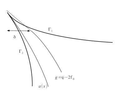
gโ€‹(x)=ฯ†โ€‹(x)โˆ’2โ€‹f0โ€‹(x).๐‘”๐‘ฅ๐œ‘๐‘ฅ2subscript๐‘“0๐‘ฅg(x)=\varphi(x)-2f_{0}(x).

Using the tangent plane formula (3.4) we compute

Lpโ€‹(x,gโ€‹(x))=โˆ’โˆซx0xfโ€ฒโ€ฒโ€‹(t)โ€‹(xโˆ’t)โ€‹๐‘‘t+12โ€‹โˆซx0xฯ†โ€ฒโ€ฒโ€‹(t)โ€‹(xโˆ’t)โ€‹๐‘‘t=โˆ’SH0โ€‹(p,(x,ฯ†โ€‹(x)))โ‰ค0subscript๐ฟ๐‘๐‘ฅ๐‘”๐‘ฅsuperscriptsubscriptsubscript๐‘ฅ0๐‘ฅsuperscript๐‘“โ€ฒโ€ฒ๐‘ก๐‘ฅ๐‘กdifferential-d๐‘ก12superscriptsubscriptsubscript๐‘ฅ0๐‘ฅsuperscript๐œ‘โ€ฒโ€ฒ๐‘ก๐‘ฅ๐‘กdifferential-d๐‘กsubscript๐‘†subscript๐ป0๐‘๐‘ฅ๐œ‘๐‘ฅ0L_{p}(x,g(x))=-\int_{x_{0}}^{x}f^{\prime\prime}(t)(x-t)\,dt+\frac{1}{2}\int_{x_{0}}^{x}\varphi^{\prime\prime}(t)(x-t)\,dt=-S_{H_{0}}(p,(x,\varphi(x)))\leq 0

by the computations in the first case. Furthermore, since f0โ€ฒโ€ฒโ‰คฯ†โ€ฒโ€ฒsuperscriptsubscript๐‘“0โ€ฒโ€ฒsuperscript๐œ‘โ€ฒโ€ฒf_{0}^{\prime\prime}\leq\varphi^{\prime\prime}, the graph of g๐‘”g lies above the function

aโ€‹(x)=โˆ’2โ€‹xโˆ’ฯ†โ€‹(x)๐‘Ž๐‘ฅ2๐‘ฅ๐œ‘๐‘ฅa(x)=-2x-\varphi(x)

defined in Proposition 3.2 (see figure 5). Since aโ€‹(x)๐‘Ž๐‘ฅa(x) lies strictly above ฮ“2subscriptฮ“2\Gamma_{2} for x>0๐‘ฅ0x>0 and โˆ‚yH0โ€‹(x0,ฯ†โ€‹(x0))=1/2subscript๐‘ฆsubscript๐ป0subscript๐‘ฅ0๐œ‘subscript๐‘ฅ012\partial_{y}H_{0}(x_{0},\varphi(x_{0}))=1/2, we have strictly positive separation on ฮ“2subscriptฮ“2\Gamma_{2}.

Refer to caption
Figure 5. The tangent plane at (x,ฯ†โ€‹(x))๐‘ฅ๐œ‘๐‘ฅ(x,\varphi(x)) is negative on the curve y=gโ€‹(x)๐‘ฆ๐‘”๐‘ฅy=g(x), hence on ฮ“2subscriptฮ“2\Gamma_{2}, for xโˆˆ[ฮด,2โˆ’ฮด]๐‘ฅ๐›ฟ2๐›ฟx\in[\delta,2-\delta].

Finally, for x0โˆˆ[1,2]subscript๐‘ฅ012x_{0}\in[1,2], the intersection of the tangent planes at p๐‘p and at p~=(2โˆ’x0,ฯ†โ€‹(2โˆ’x0))~๐‘2subscript๐‘ฅ0๐œ‘2subscript๐‘ฅ0\tilde{p}=(2-x_{0},\varphi(2-x_{0})) is the line x=1๐‘ฅ1x=1 since f0โ€ฒโ€ฒsuperscriptsubscript๐‘“0โ€ฒโ€ฒf_{0}^{\prime\prime} is symmetric around x=1๐‘ฅ1x=1. By the previous computations, the tangent plane at p~~๐‘\tilde{p} is negative on ฮ“2subscriptฮ“2\Gamma_{2}. Thus, the tangent plane at p๐‘p is negative on ฮ“2subscriptฮ“2\Gamma_{2}, completing the proof. โˆŽ

3.6. Proof of Key Proposition

We can slightly modify the construction of H0subscript๐ป0H_{0} from the previous section to make it smooth, at the expense of giving up a little convexity near the cusps of ฮ“ฮ“\Gamma. Below ฮด,ฮณ>0๐›ฟ๐›พ0\delta,\,\gamma>0 are small constants depending only on ฯ†๐œ‘\varphi. Let Gโ€‹(p1,p2,p3)=Hโ€‹(p1,p22+p32)๐บsubscript๐‘1subscript๐‘2subscript๐‘3๐ปsubscript๐‘1superscriptsubscript๐‘22superscriptsubscript๐‘32G(p_{1},p_{2},p_{3})=H\left(p_{1},\sqrt{p_{2}^{2}+p_{3}^{2}}\right).

Proposition 3.11.

For any ฯต>0italic-ฯต0\epsilon>0 there exists a smooth function H๐ปH defined on a neighborhood of ฮ“ฮ“\Gamma such that

  1. (1)

    H๐ปH is linear (depending only on x๐‘ฅx) in a neighborhood of ฮ“2subscriptฮ“2\Gamma_{2}, respectively ฮ“4subscriptฮ“4\Gamma_{4},

  2. (2)

    divโ€‹(โˆ‡Gโ€‹(โˆ‡u0))=0divโˆ‡๐บโˆ‡subscript๐‘ข00\text{div}(\nabla G(\nabla u_{0}))=0,

  3. (3)

    Hyโ€‹(x,ฯ†โ€‹(x))โ‰ฅ12subscript๐ป๐‘ฆ๐‘ฅ๐œ‘๐‘ฅ12H_{y}(x,\varphi(x))\geq\frac{1}{2} for xโˆˆ[ฮด,2โˆ’ฮด]๐‘ฅ๐›ฟ2๐›ฟx\in[\delta,2-\delta], and Hyโ‰ฅ0subscript๐ป๐‘ฆ0H_{y}\geq 0 on ฮ“1subscriptฮ“1\Gamma_{1},

  4. (4)

    If p=(x,ฯ†โ€‹(x))๐‘๐‘ฅ๐œ‘๐‘ฅp=(x,\varphi(x)) with xโˆˆ[ฮด,2โˆ’ฮด]๐‘ฅ๐›ฟ2๐›ฟx\in[\delta,2-\delta] then SHโ€‹(p,q)โ‰ฅฮณโ€‹|pโˆ’q|2subscript๐‘†๐ป๐‘๐‘ž๐›พsuperscript๐‘๐‘ž2S_{H}(p,q)\geq\gamma|p-q|^{2} for all qโˆˆฮ“๐‘žฮ“q\in\Gamma,

  5. (5)

    SHโ€‹(p,q)โ‰ฅโˆ’ฯตโ€‹|pโˆ’q|2subscript๐‘†๐ป๐‘๐‘žitalic-ฯตsuperscript๐‘๐‘ž2S_{H}(p,q)\geq-\epsilon|p-q|^{2} otherwise for p,qโˆˆฮ“๐‘๐‘žฮ“p,\,q\in\Gamma.

Note that the key Proposition 2.4 follows easily from Proposition 3.11 by defining G๐บG as above.

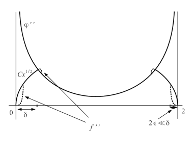
Let ฮฑ=12๐›ผ12\alpha=\frac{1}{2} in the construction of f0โ€ฒโ€ฒsuperscriptsubscript๐‘“0โ€ฒโ€ฒf_{0}^{\prime\prime} from the previous section and let ฯตโ‰ชฮดmuch-less-thanitalic-ฯต๐›ฟ\epsilon\ll\delta. Let fโ€ฒโ€ฒsuperscript๐‘“โ€ฒโ€ฒf^{\prime\prime} be a smoothing of f0โ€ฒโ€ฒsuperscriptsubscript๐‘“0โ€ฒโ€ฒf_{0}^{\prime\prime} defined by cutting it off smoothly to zero between ฯตitalic-ฯต\epsilon and 2โ€‹ฯต2italic-ฯต2\epsilon, gluing it smoothly to itself between ฮด๐›ฟ\delta and ฮด+ฯต๐›ฟitalic-ฯต\delta+\epsilon, and making it symmetric over x=1๐‘ฅ1x=1 (see figure 6). Let H๐ปH be the function in (3.1) determined by f๐‘“f through the Euler-Lagrange relation (3.3).

Refer to caption
Figure 6. fโ€ฒโ€ฒsuperscript๐‘“โ€ฒโ€ฒf^{\prime\prime} is a small perturbation of f0โ€ฒโ€ฒsuperscriptsubscript๐‘“0โ€ฒโ€ฒf_{0}^{\prime\prime} that connects smoothly to ฯ†โ€ฒโ€ฒsuperscript๐œ‘โ€ฒโ€ฒ\varphi^{\prime\prime} near x=ฮด๐‘ฅ๐›ฟx=\delta and goes quickly to zero near x=0๐‘ฅ0x=0.
Proof of proposition 3.11.

The first three conclusions are clear by construction so we just need to check the convexity conclusions. Most of them will follow by continuity.

If pโˆˆฮ“2๐‘subscriptฮ“2p\in\Gamma_{2} we have positive separation since Hโ‰ฅ0๐ป0H\geq 0, so assume p=(x0,ฯ†โ€‹(x0))๐‘subscript๐‘ฅ0๐œ‘subscript๐‘ฅ0p=(x_{0},\varphi(x_{0})).

If x0โˆˆ[ฮด,2โˆ’ฮด]subscript๐‘ฅ0๐›ฟ2๐›ฟx_{0}\in[\delta,2-\delta] then the conclusion holds by continuity from the arguments in the proof of Proposition 3.10 after taking ฯตitalic-ฯต\epsilon small.

Next we may assume by symmetry that x0โˆˆ[0,ฮด]subscript๐‘ฅ00๐›ฟx_{0}\in[0,\delta].

Case 1: Assume that x0โ‰ฅ10โ€‹ฯตsubscript๐‘ฅ010italic-ฯตx_{0}\geq 10\epsilon.

If q=(x,ฯ†โ€‹(x))๐‘ž๐‘ฅ๐œ‘๐‘ฅq=(x,\varphi(x)) with x>x0๐‘ฅsubscript๐‘ฅ0x>x_{0} then the positive separation follows again by continuity. If x<x0๐‘ฅsubscript๐‘ฅ0x<x_{0} one computes

2โ€‹sfโ€ฒโ€ฒโ€‹(x0,x)โ‰ฅ2โ€‹sfโ€ฒโ€ฒโ€‹(x0,0)โ‰ฅ45โ€‹(1โˆ’(1/5)5/2)>sฯ†โ€ฒโ€ฒโ€‹(x0,0)โ‰ฅsฯ†โ€ฒโ€ฒโ€‹(x0,x)2subscript๐‘ superscript๐‘“โ€ฒโ€ฒsubscript๐‘ฅ0๐‘ฅ2subscript๐‘ superscript๐‘“โ€ฒโ€ฒsubscript๐‘ฅ00451superscript1552subscript๐‘ superscript๐œ‘โ€ฒโ€ฒsubscript๐‘ฅ00subscript๐‘ superscript๐œ‘โ€ฒโ€ฒsubscript๐‘ฅ0๐‘ฅ2s_{f^{\prime\prime}}(x_{0},x)\geq 2s_{f^{\prime\prime}}(x_{0},0)\geq\frac{4}{5}(1-(1/5)^{5/2})>s_{\varphi^{\prime\prime}}(x_{0},0)\geq s_{\varphi^{\prime\prime}}(x_{0},x)

so condition (3.7) holds and we have positive separation on ฮ“1subscriptฮ“1\Gamma_{1}.

Since the cutoff is between ฯตitalic-ฯต\epsilon and 2โ€‹ฯต2italic-ฯต2\epsilon and fโ€ฒโ€ฒsuperscript๐‘“โ€ฒโ€ฒf^{\prime\prime} is increasing for x<ฮด๐‘ฅ๐›ฟx<\delta we compute

(3.10) dfโ€ฒโ€ฒโ€‹(x0)<23.subscript๐‘‘superscript๐‘“โ€ฒโ€ฒsubscript๐‘ฅ023d_{f^{\prime\prime}}(x_{0})<\frac{2}{3}.

and by Remark 3.8 the condition (3.9) holds for x0<ฮดsubscript๐‘ฅ0๐›ฟx_{0}<\delta. We thus have positive separation on ฮ“2subscriptฮ“2\Gamma_{2} and ฮ“3subscriptฮ“3\Gamma_{3}.

Finally, for qโˆˆฮ“4๐‘žsubscriptฮ“4q\in\Gamma_{4} positive separation follows again by continuity.

This establishes positive separation everywhere for x0โˆˆ[10โ€‹ฯต,2โˆ’10โ€‹ฯต]subscript๐‘ฅ010italic-ฯต210italic-ฯตx_{0}\in[10\epsilon,2-10\epsilon].

Case 2: Assume x0โ‰ค10โ€‹ฯตsubscript๐‘ฅ010italic-ฯตx_{0}\leq 10\epsilon.

The tangent plane at p๐‘p is of order ฯตitalic-ฯต\epsilon on ฮ“ฮ“\Gamma, so we have positive separation when qโˆˆฮ“4๐‘žsubscriptฮ“4q\in\Gamma_{4}.

Using that fโ€ฒโ€ฒsuperscript๐‘“โ€ฒโ€ฒf^{\prime\prime} is increasing and ฯ†โ€ฒโ€ฒsuperscript๐œ‘โ€ฒโ€ฒ\varphi^{\prime\prime} decreasing near 00, we obtain positive separation if q=(x,ฯ†โ€‹(x))๐‘ž๐‘ฅ๐œ‘๐‘ฅq=(x,\varphi(x)) with xโˆˆ[x0,ฮด]๐‘ฅsubscript๐‘ฅ0๐›ฟx\in[x_{0},\delta]. The same holds for x>ฮด๐‘ฅ๐›ฟx>\delta by continuity.

If q=(x,ฯ†โ€‹(x))๐‘ž๐‘ฅ๐œ‘๐‘ฅq=(x,\varphi(x)) for x<x0๐‘ฅsubscript๐‘ฅ0x<x_{0} we compute

SHโ€‹(p,q)โ‰ฅโˆ’fโ€ฒโ€ฒโ€‹(x0)โ€‹sฯ†โ€ฒโ€ฒโ€‹(x0,x)โ€‹(xโˆ’x0)2โ‰ฅโˆ’Cโ€‹ฯตโ€‹|pโˆ’q|2,subscript๐‘†๐ป๐‘๐‘žsuperscript๐‘“โ€ฒโ€ฒsubscript๐‘ฅ0subscript๐‘ superscript๐œ‘โ€ฒโ€ฒsubscript๐‘ฅ0๐‘ฅsuperscript๐‘ฅsubscript๐‘ฅ02๐ถitalic-ฯตsuperscript๐‘๐‘ž2S_{H}(p,q)\geq-f^{\prime\prime}(x_{0})s_{\varphi^{\prime\prime}}(x_{0},x)(x-x_{0})^{2}\geq-C\sqrt{\epsilon}\,\,|p-q|^{2},

since sฯ†โ€ฒโ€ฒโ€‹(x0,x)โ‰คsฯ†โ€ฒโ€ฒโ€‹(x0,0)โ‰ค1subscript๐‘ superscript๐œ‘โ€ฒโ€ฒsubscript๐‘ฅ0๐‘ฅsubscript๐‘ superscript๐œ‘โ€ฒโ€ฒsubscript๐‘ฅ001s_{\varphi^{\prime\prime}}(x_{0},x)\leq s_{\varphi^{\prime\prime}}(x_{0},0)\leq 1. This gives the desired estimate on ฮ“1subscriptฮ“1\Gamma_{1}.

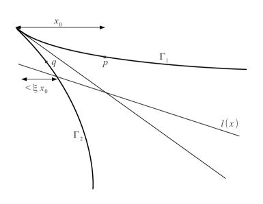
Next we bound SHโ€‹(p,q)subscript๐‘†๐ป๐‘๐‘žS_{H}(p,q) with qโˆˆฮ“2๐‘žsubscriptฮ“2q\in\Gamma_{2}. For this we estimate the location of the intersection line lpsubscript๐‘™๐‘l_{p} of the tangent plane at p๐‘p with 00. By (3.8), lpsubscript๐‘™๐‘l_{p} passes through

(x0,ฯ†โ€‹(x0)โˆ’2โ€‹ฯ†โ€ฒโ€ฒโ€‹(x0)fโ€ฒโ€ฒโ€‹(x0)โ€‹โˆซ0x0(x0โˆ’t)โ€‹fโ€ฒโ€ฒโ€‹(t)โ€‹๐‘‘t).subscript๐‘ฅ0๐œ‘subscript๐‘ฅ02superscript๐œ‘โ€ฒโ€ฒsubscript๐‘ฅ0superscript๐‘“โ€ฒโ€ฒsubscript๐‘ฅ0superscriptsubscript0subscript๐‘ฅ0subscript๐‘ฅ0๐‘กsuperscript๐‘“โ€ฒโ€ฒ๐‘กdifferential-d๐‘ก\left(x_{0},\varphi(x_{0})-\frac{2\varphi^{\prime\prime}(x_{0})}{f^{\prime\prime}(x_{0})}\int_{0}^{x_{0}}(x_{0}-t)f^{\prime\prime}(t)\,dt\right).

We first claim that this point lies above the line y=โˆ’x๐‘ฆ๐‘ฅy=-x. Indeed, since fโ€ฒโ€ฒsuperscript๐‘“โ€ฒโ€ฒf^{\prime\prime} is increasing in [0,x0]0subscript๐‘ฅ0[0,x_{0}], the second component is larger than ฯ†โ€‹(x0)โˆ’ฯ†โ€ฒโ€ฒโ€‹(x0)โ€‹x02๐œ‘subscript๐‘ฅ0superscript๐œ‘โ€ฒโ€ฒsubscript๐‘ฅ0superscriptsubscript๐‘ฅ02\varphi(x_{0})-\varphi^{\prime\prime}(x_{0})x_{0}^{2}, and using the expansion (3.2) we see that

ฯ†โ€‹(x0)+x0โ‰ฅ(43โ€‹ฯ†โ€ฒโ€ฒโ€‹(x0)+Oโ€‹(1))โ€‹x02>ฯ†โ€ฒโ€ฒโ€‹(x0)โ€‹x02.๐œ‘subscript๐‘ฅ0subscript๐‘ฅ043superscript๐œ‘โ€ฒโ€ฒsubscript๐‘ฅ0๐‘‚1superscriptsubscript๐‘ฅ02superscript๐œ‘โ€ฒโ€ฒsubscript๐‘ฅ0superscriptsubscript๐‘ฅ02\varphi(x_{0})+x_{0}\geq\left(\frac{4}{3}\varphi^{\prime\prime}(x_{0})+O(1)\right)x_{0}^{2}>\varphi^{\prime\prime}(x_{0})x_{0}^{2}.

By (3.10) the slope of lpsubscript๐‘™๐‘l_{p} is between โˆ’11-1 and 00, so we have positive separation for qโˆˆฮ“3๐‘žsubscriptฮ“3q\in\Gamma_{3} and qโˆˆฮ“2โˆฉ{y<โˆ’x0}๐‘žsubscriptฮ“2๐‘ฆsubscript๐‘ฅ0q\in\Gamma_{2}\cap\{y<-x_{0}\}.

Finally, from (3.8) we see that the slope of lpsubscript๐‘™๐‘l_{p} is less than ฯ†โ€ฒโ€‹(x0)superscript๐œ‘โ€ฒsubscript๐‘ฅ0\varphi^{\prime}(x_{0}). Thus, for x<x0๐‘ฅsubscript๐‘ฅ0x<x_{0}, lpsubscript๐‘™๐‘l_{p} lies above the line

y=lโ€‹(x)=โˆ’x0+ฯ†โ€ฒโ€‹(x0)โ€‹(xโˆ’x0).๐‘ฆ๐‘™๐‘ฅsubscript๐‘ฅ0superscript๐œ‘โ€ฒsubscript๐‘ฅ0๐‘ฅsubscript๐‘ฅ0y=l(x)=-x_{0}+\varphi^{\prime}(x_{0})(x-x_{0}).

A short computation using the expansion (3.2) shows that lโ€‹(x)๐‘™๐‘ฅl(x) crosses aโ€‹(x)๐‘Ž๐‘ฅa(x), hence ฮ“2subscriptฮ“2\Gamma_{2}, at some x<ฮพโ€‹x0๐‘ฅ๐œ‰subscript๐‘ฅ0x<\xi x_{0} where

ฮพ+23โ€‹ฮพ3/2=1+Oโ€‹(ฯต).๐œ‰23superscript๐œ‰321๐‘‚italic-ฯต\xi+\frac{2}{3}\xi^{3/2}=1+O(\sqrt{\epsilon}).

In particular, ฮพ<1โˆ’c๐œ‰1๐‘\xi<1-c. This gives that the separation is positive on ฮ“2โˆฉ{x>ฮพโ€‹x0}subscriptฮ“2๐‘ฅ๐œ‰subscript๐‘ฅ0\Gamma_{2}\cap\{x>\xi x_{0}\}, and otherwise the separation is at worst โˆ’Cโ€‹ฯตโ€‹x02โ‰ฅโˆ’Cโ€‹ฯตโ€‹|pโˆ’q|2๐ถitalic-ฯตsuperscriptsubscript๐‘ฅ02๐ถitalic-ฯตsuperscript๐‘๐‘ž2-C\sqrt{\epsilon}x_{0}^{2}\geq-C\sqrt{\epsilon}|p-q|^{2} (see figure 7).

โˆŽ

Refer to caption
Figure 7. The separation is positive if q๐‘žq is below the line lโ€‹(x)๐‘™๐‘ฅl(x), and if the separation is negative then |pโˆ’q|๐‘๐‘ž|p-q| is of order x0subscript๐‘ฅ0x_{0}.
Remark 3.12.

The proof shows in fact that SHโ€‹(p,q)subscript๐‘†๐ป๐‘๐‘žS_{H}(p,q) is only negative for p,q๐‘๐‘žp,\,q very close to the same cusp.

4. Appendix

4.1. Convex Extension Lemma

Proof of lemma 2.1.

Let ๐ฏTsubscript๐ฏ๐‘‡{\bf v}_{T} be the tangential component and ๐ฏโŸ‚subscript๐ฏperpendicular-to{\bf v}_{\perp} be the normal component, and let โˆ‡ฮฃGsuperscriptโˆ‡ฮฃ๐บ\nabla^{\Sigma}G be the gradient of G๐บG on ฮฃฮฃ\Sigma. Note that condition 2.1 implies ๐ฏT=โˆ‡ฮฃGsubscript๐ฏ๐‘‡superscriptโˆ‡ฮฃ๐บ{\bf v}_{T}=\nabla^{\Sigma}G. For xโˆˆฮฃ๐‘ฅฮฃx\in\Sigma let Tx,Nxsubscript๐‘‡๐‘ฅsubscript๐‘๐‘ฅT_{x},\,N_{x} be the tangent and normal subspaces to ฮฃฮฃ\Sigma at x๐‘ฅx. Let dฮฃโ€‹(y)subscript๐‘‘ฮฃ๐‘ฆd_{\Sigma}(y) be the distance from y๐‘ฆy to ฮฃฮฃ\Sigma and let

ฮฃr={y:dฮฃโ€‹(y)<r}.superscriptฮฃ๐‘Ÿconditional-set๐‘ฆsubscript๐‘‘ฮฃ๐‘ฆ๐‘Ÿ\Sigma^{r}=\{y:d_{\Sigma}(y)<r\}.

Finally, for xโˆˆโ„n๐‘ฅsuperscriptโ„๐‘›x\in\mathbb{R}^{n} let yโ€‹(x)๐‘ฆ๐‘ฅy(x) be the closest point in ฮฃฮฃ\Sigma to x๐‘ฅx. It is well-known that y๐‘ฆy and dฮฃ2superscriptsubscript๐‘‘ฮฃ2d_{\Sigma}^{2} are well-defined and smooth in a neighborhood of ฮฃฮฃ\Sigma, and for xโˆˆฮฃ๐‘ฅฮฃx\in\Sigma, Dxโ€‹yโ€‹(x)subscript๐ท๐‘ฅ๐‘ฆ๐‘ฅD_{x}y(x) is the projection to Txsubscript๐‘‡๐‘ฅT_{x} and D2โ€‹(dฮฃ2/2)โ€‹(x)superscript๐ท2superscriptsubscript๐‘‘ฮฃ22๐‘ฅD^{2}(d_{\Sigma}^{2}/2)(x) is the projection to Nxsubscript๐‘๐‘ฅN_{x}. (For proofs, see for example [AS]).

Step 1: We claim that the function

Fโ€‹(x)=Gโ€‹(yโ€‹(x))+๐ฏโ€‹(yโ€‹(x))โ‹…(xโˆ’yโ€‹(x))+A2โ€‹dฮฃ2โ€‹(x)๐น๐‘ฅ๐บ๐‘ฆ๐‘ฅโ‹…๐ฏ๐‘ฆ๐‘ฅ๐‘ฅ๐‘ฆ๐‘ฅ๐ด2superscriptsubscript๐‘‘ฮฃ2๐‘ฅF(x)=G(y(x))+{\bf v}(y(x))\cdot(x-y(x))+\frac{A}{2}d_{\Sigma}^{2}(x)

with A๐ดA large lifts quadratically from its tangent planes in ฮฃฯƒsuperscriptฮฃ๐œŽ\Sigma^{\sigma} for ฯƒ๐œŽ\sigma sufficiently small. We first compute for xโˆˆฮฃ๐‘ฅฮฃx\in\Sigma that

Fโ€‹(x+ฯตโ€‹z)๐น๐‘ฅitalic-ฯต๐‘ง\displaystyle F(x+\epsilon z) =Gโ€‹(x)+ฯตโ€‹(โˆ‡ฮฃGโ€‹(x)โ‹…zT+๐ฏโ€‹(x)โ‹…zโŸ‚)+Oโ€‹(ฯต2)absent๐บ๐‘ฅitalic-ฯตโ‹…superscriptโˆ‡ฮฃ๐บ๐‘ฅsubscript๐‘ง๐‘‡โ‹…๐ฏ๐‘ฅsubscript๐‘งperpendicular-to๐‘‚superscriptitalic-ฯต2\displaystyle=G(x)+\epsilon\left(\nabla^{\Sigma}G(x)\cdot z_{T}+{\bf v}(x)\cdot z_{\perp}\right)+O(\epsilon^{2})
=Gโ€‹(x)+ฯตโ€‹๐ฏโ€‹(x)โ‹…z+Oโ€‹(ฯต2)absent๐บ๐‘ฅโ‹…italic-ฯต๐ฏ๐‘ฅ๐‘ง๐‘‚superscriptitalic-ฯต2\displaystyle=G(x)+\epsilon{\bf v}(x)\cdot z+O(\epsilon^{2})

giving that F=G๐น๐บF=G on ฮฃฮฃ\Sigma and โˆ‡F=๐ฏโˆ‡๐น๐ฏ\nabla F={\bf v} on ฮฃฮฃ\Sigma.

Now, for ฯตitalic-ฯต\epsilon small and ฮฝโˆˆNx๐œˆsubscript๐‘๐‘ฅ\nu\in N_{x} we have yโ€‹(x+ฯตโ€‹ฮฝ)=x๐‘ฆ๐‘ฅitalic-ฯต๐œˆ๐‘ฅy(x+\epsilon\nu)=x and dฮฃโ€‹(x+ฯตโ€‹ฮฝ)=ฯตsubscript๐‘‘ฮฃ๐‘ฅitalic-ฯต๐œˆitalic-ฯตd_{\Sigma}(x+\epsilon\nu)=\epsilon, so Fฮฝโ€‹ฮฝโ€‹(x)=A.subscript๐น๐œˆ๐œˆ๐‘ฅ๐ดF_{\nu\nu}(x)=A. In addition, if xโˆˆฮฃ๐‘ฅฮฃx\in\Sigma and x+ฯตโ€‹zโˆˆฮฃ๐‘ฅitalic-ฯต๐‘งฮฃx+\epsilon z\in\Sigma for some unit vector z๐‘งz then by hypothesis we have

Fโ€‹(x+ฯตโ€‹z)๐น๐‘ฅitalic-ฯต๐‘ง\displaystyle F(x+\epsilon z) =Fโ€‹(x)+ฯตโ€‹โˆ‡Fโ€‹(x)โ‹…z+ฯต22โ€‹zTโ‹…D2โ€‹Fโ€‹(x)โ‹…z+Oโ€‹(ฯต3)absent๐น๐‘ฅโ‹…italic-ฯตโˆ‡๐น๐‘ฅ๐‘งโ‹…โ‹…superscriptitalic-ฯต22superscript๐‘ง๐‘‡superscript๐ท2๐น๐‘ฅ๐‘ง๐‘‚superscriptitalic-ฯต3\displaystyle=F(x)+\epsilon\nabla F(x)\cdot z+\frac{\epsilon^{2}}{2}z^{T}\cdot D^{2}F(x)\cdot z+O(\epsilon^{3})
โ‰ฅFโ€‹(x)+ฯตโ€‹โˆ‡Fโ€‹(x)โ‹…z+ฮณโ€‹ฯต2.absent๐น๐‘ฅโ‹…italic-ฯตโˆ‡๐น๐‘ฅ๐‘ง๐›พsuperscriptitalic-ฯต2\displaystyle\geq F(x)+\epsilon\nabla F(x)\cdot z+\gamma\epsilon^{2}.

Taking ฯตitalic-ฯต\epsilon to zero we see that Fฯ„โ€‹ฯ„โ€‹(x)>2โ€‹ฮณsubscript๐น๐œ๐œ๐‘ฅ2๐›พF_{\tau\tau}(x)>2\gamma for any tangential unit vector ฯ„๐œ\tau.

Take any unit vector e๐‘’e and write e=ฮฑโ€‹ฯ„+1โˆ’ฮฑ2โ€‹ฮฝ๐‘’๐›ผ๐œ1superscript๐›ผ2๐œˆe=\alpha\tau+\sqrt{1-\alpha^{2}}\nu for some unit ฯ„โˆˆTxโ€‹ฮฃ๐œsubscript๐‘‡๐‘ฅฮฃ\tau\in T_{x}\Sigma and ฮฝโˆˆNxโ€‹ฮฃ๐œˆsubscript๐‘๐‘ฅฮฃ\nu\in N_{x}\Sigma. Since D2โ€‹(dฮฃ2/2)superscript๐ท2superscriptsubscript๐‘‘ฮฃ22D^{2}(d_{\Sigma}^{2}/2) is the projection matrix onto Nxsubscript๐‘๐‘ฅN_{x} at xโˆˆฮฃ๐‘ฅฮฃx\in\Sigma, we have

Feโ€‹eโ€‹(x)subscript๐น๐‘’๐‘’๐‘ฅ\displaystyle F_{ee}(x) =ฮฑ2โ€‹Fฯ„โ€‹ฯ„+(1โˆ’ฮฑ2)โ€‹Fฮฝโ€‹ฮฝ+2โ€‹ฮฑโ€‹1โˆ’ฮฑ2โ€‹(Fโˆ’Aโ€‹dฮฃ2/2)ฯ„โ€‹ฮฝabsentsuperscript๐›ผ2subscript๐น๐œ๐œ1superscript๐›ผ2subscript๐น๐œˆ๐œˆ2๐›ผ1superscript๐›ผ2subscript๐น๐ดsuperscriptsubscript๐‘‘ฮฃ22๐œ๐œˆ\displaystyle=\alpha^{2}F_{\tau\tau}+(1-\alpha^{2})F_{\nu\nu}+2\alpha\sqrt{1-\alpha^{2}}(F-Ad_{\Sigma}^{2}/2)_{\tau\nu}
โ‰ฅ2โ€‹ฮฑ2โ€‹ฮณ+(1โˆ’ฮฑ2)โ€‹Aโˆ’Cโ€‹ฮฑโ€‹1โˆ’ฮฑ2absent2superscript๐›ผ2๐›พ1superscript๐›ผ2๐ด๐ถ๐›ผ1superscript๐›ผ2\displaystyle\geq 2\alpha^{2}\gamma+(1-\alpha^{2})A-C\alpha\sqrt{1-\alpha^{2}}

for some C๐ถC independent of A๐ดA. We conclude that D2โ€‹F>32โ€‹ฮณโ€‹Isuperscript๐ท2๐น32๐›พ๐ผD^{2}F>\frac{3}{2}\gamma I on ฮฃฮฃ\Sigma for A๐ดA sufficiently large, and in particular, D2โ€‹F>32โ€‹ฮณโ€‹Isuperscript๐ท2๐น32๐›พ๐ผD^{2}F>\frac{3}{2}\gamma I on a neighborhood ฮฃ2โ€‹ฯsuperscriptฮฃ2๐œŒ\Sigma^{2\rho} of ฮฃฮฃ\Sigma.

Finally, we show that the tangent planes to F๐นF in ฮฃฯƒsuperscriptฮฃ๐œŽ\Sigma^{\sigma} separate quadratically for ฯƒ๐œŽ\sigma small. Let x,zโˆˆฮฃฯƒ๐‘ฅ๐‘งsuperscriptฮฃ๐œŽx,\,z\in\Sigma^{\sigma}. We divide into two cases.

If |zโˆ’x|<ฯ๐‘ง๐‘ฅ๐œŒ|z-x|<\rho then x๐‘ฅx and z๐‘งz can be connected by a line segment contained in ฮฃ2โ€‹ฯsuperscriptฮฃ2๐œŒ\Sigma^{2\rho}, so it is clear that

Fโ€‹(z)>Fโ€‹(x)+โˆ‡Fโ€‹(x)โ‹…(zโˆ’x)+34โ€‹ฮณโ€‹|zโˆ’x|2.๐น๐‘ง๐น๐‘ฅโ‹…โˆ‡๐น๐‘ฅ๐‘ง๐‘ฅ34๐›พsuperscript๐‘ง๐‘ฅ2F(z)>F(x)+\nabla F(x)\cdot(z-x)+\frac{3}{4}\gamma|z-x|^{2}.

If on the other hand |zโˆ’x|>ฯ๐‘ง๐‘ฅ๐œŒ|z-x|>\rho, we use that

Fโ€‹(yโ€‹(z))>Fโ€‹(yโ€‹(x))+โˆ‡Fโ€‹(yโ€‹(x))โ‹…(yโ€‹(z)โˆ’yโ€‹(x))+ฮณโ€‹|yโ€‹(z)โˆ’yโ€‹(x)|2.๐น๐‘ฆ๐‘ง๐น๐‘ฆ๐‘ฅโ‹…โˆ‡๐น๐‘ฆ๐‘ฅ๐‘ฆ๐‘ง๐‘ฆ๐‘ฅ๐›พsuperscript๐‘ฆ๐‘ง๐‘ฆ๐‘ฅ2F(y(z))>F(y(x))+\nabla F(y(x))\cdot(y(z)-y(x))+\gamma|y(z)-y(x)|^{2}.

Replacing yโ€‹(z)๐‘ฆ๐‘งy(z) by z๐‘งz and yโ€‹(x)๐‘ฆ๐‘ฅy(x) by x๐‘ฅx changes these quantities by at most Cโ€‹ฯƒ๐ถ๐œŽC\sigma, and since and |zโˆ’x|>ฯ๐‘ง๐‘ฅ๐œŒ|z-x|>\rho we have that

Fโ€‹(z)>Fโ€‹(x)+โˆ‡Fโ€‹(x)โ‹…(zโˆ’x)+34โ€‹ฮณโ€‹|zโˆ’x|2๐น๐‘ง๐น๐‘ฅโ‹…โˆ‡๐น๐‘ฅ๐‘ง๐‘ฅ34๐›พsuperscript๐‘ง๐‘ฅ2F(z)>F(x)+\nabla F(x)\cdot(z-x)+\frac{3}{4}\gamma|z-x|^{2}

for all x,zโˆˆฮฃฯƒ๐‘ฅ๐‘งsuperscriptฮฃ๐œŽx,\,z\in\Sigma^{\sigma} for ฯƒ๐œŽ\sigma small.

Step 2: From now on denote the open set ฮฃฯƒsuperscriptฮฃ๐œŽ\Sigma^{\sigma} by N๐‘N. Let Nฯตsubscript๐‘italic-ฯตN_{\epsilon} denote {xโˆˆN:Bฯตโ€‹(x)โŠ‚N}conditional-set๐‘ฅ๐‘subscript๐ตitalic-ฯต๐‘ฅ๐‘\{x\in N:B_{\epsilon}(x)\subset N\}. Finally, let ฯฯตsubscript๐œŒitalic-ฯต\rho_{\epsilon} denote the standard mollifier ฯตโˆ’nโ€‹ฯโ€‹(x/ฯต)superscriptitalic-ฯต๐‘›๐œŒ๐‘ฅitalic-ฯต\epsilon^{-n}\rho(x/\epsilon) where ฯ๐œŒ\rho is supported in B1subscript๐ต1B_{1}, nonnegative, smooth and has unit mass.

We define a global uniformly convex function that agrees with F๐นF on N๐‘N. Let

H0โ€‹(y)=supxโˆˆN{Fโ€‹(x)+โˆ‡Fโ€‹(x)โ‹…(yโˆ’x)+34โ€‹ฮณโ€‹|yโˆ’x|2}.subscript๐ป0๐‘ฆsubscriptsupremum๐‘ฅ๐‘๐น๐‘ฅโ‹…โˆ‡๐น๐‘ฅ๐‘ฆ๐‘ฅ34๐›พsuperscript๐‘ฆ๐‘ฅ2H_{0}(y)=\sup_{x\in N}\left\{F(x)+\nabla F(x)\cdot(y-x)+\frac{3}{4}\gamma|y-x|^{2}\right\}.

Then H0subscript๐ป0H_{0} is a uniformly convex function on โ„nsuperscriptโ„๐‘›\mathbb{R}^{n} with D2โ€‹H0โ‰ฅ32โ€‹ฮณโ€‹Isuperscript๐ท2subscript๐ป032๐›พ๐ผD^{2}H_{0}\geq\frac{3}{2}\gamma I and furthermore by construction we have that H0=Fsubscript๐ป0๐นH_{0}=F on N๐‘N.

To finish we glue H0subscript๐ป0H_{0} to a mollification. Fix ฮด๐›ฟ\delta so that ฮฃโŠ‚N2โ€‹ฮดฮฃsubscript๐‘2๐›ฟ\Sigma\subset N_{2\delta}. Let

Hฯต=ฯฯตโˆ—H0subscript๐ปitalic-ฯตโˆ—subscript๐œŒitalic-ฯตsubscript๐ป0H_{\epsilon}=\rho_{\epsilon}\ast H_{0}

for some ฯตitalic-ฯต\epsilon small. In Nฮดsubscript๐‘๐›ฟN_{\delta} we have

|Hฯตโˆ’H0|,|โˆ‡Hฯตโˆ’โˆ‡H0|<Cโ€‹ฯต.subscript๐ปitalic-ฯตsubscript๐ป0โˆ‡subscript๐ปitalic-ฯตโˆ‡subscript๐ป0๐ถitalic-ฯต|H_{\epsilon}-H_{0}|,\,|\nabla H_{\epsilon}-\nabla H_{0}|<C\epsilon.

Finally, since D2โ€‹H0โ‰ฅ32โ€‹ฮณโ€‹Isuperscript๐ท2subscript๐ป032๐›พ๐ผD^{2}H_{0}\geq\frac{3}{2}\gamma I we have D2โ€‹Hฯต>32โ€‹ฮณโ€‹I.superscript๐ท2subscript๐ปitalic-ฯต32๐›พ๐ผD^{2}H_{\epsilon}>\frac{3}{2}\gamma I.

Let ฮท๐œ‚\eta be a smooth cutoff function which is 111 on N2โ€‹ฮดsubscript๐‘2๐›ฟN_{2\delta} and 00 outside of Nฮดsubscript๐‘๐›ฟN_{\delta}. Then let

H=ฮทโ€‹H0+(1โˆ’ฮท)โ€‹Hฯต.๐ป๐œ‚subscript๐ป01๐œ‚subscript๐ปitalic-ฯตH=\eta H_{0}+(1-\eta)H_{\epsilon}.

We compute

D2โ€‹H=ฮทโ€‹D2โ€‹H0+(1โˆ’ฮท)โ€‹D2โ€‹Hฯต+2โ€‹โˆ‡ฮทโŠ—โˆ‡(H0โˆ’Hฯต)+D2โ€‹ฮทโ€‹(H0โˆ’Hฯต).superscript๐ท2๐ป๐œ‚superscript๐ท2subscript๐ป01๐œ‚superscript๐ท2subscript๐ปitalic-ฯตtensor-product2โˆ‡๐œ‚โˆ‡subscript๐ป0subscript๐ปitalic-ฯตsuperscript๐ท2๐œ‚subscript๐ป0subscript๐ปitalic-ฯตD^{2}H=\eta D^{2}H_{0}+(1-\eta)D^{2}H_{\epsilon}+2\nabla\eta\otimes\nabla(H_{0}-H_{\epsilon})+D^{2}\eta(H_{0}-H_{\epsilon}).

Then H๐ปH is smooth, H=F๐ป๐นH=F on N2โ€‹ฮดsubscript๐‘2๐›ฟN_{2\delta} and taking ฯตitalic-ฯต\epsilon small we have D2โ€‹H>ฮณโ€‹Isuperscript๐ท2๐ป๐›พ๐ผD^{2}H>\gamma I, completing the construction. โˆŽ

4.2. Expansion of ฯ†๐œ‘\varphi

Proof of proposition 3.1.

The symmetries of ฯ†๐œ‘\varphi follow from the symmetries of w๐‘คw.

The curve ฮ“1subscriptฮ“1\Gamma_{1} is parametrized by โˆ‡wโ€‹(ฮธ)โˆ‡๐‘ค๐œƒ\nabla w(\theta) for ฮธโˆˆ[ฯ€/4,โ€‰3โ€‹ฯ€/4]๐œƒ๐œ‹43๐œ‹4\theta\in[\pi/4,\,3\pi/4]. Let ฮฝ๐œˆ\nu be the upward normal to ฮ“1subscriptฮ“1\Gamma_{1}. Since w๐‘คw is homogeneous degree one we have ฮฝโ€‹(โˆ‡wโ€‹(ฮธ))=ฮธ๐œˆโˆ‡๐‘ค๐œƒ๐œƒ\nu(\nabla w(\theta))=\theta. Differentiating we get the the curvature ฮบ=1gโ€ฒโ€ฒ+g๐œ…1superscript๐‘”โ€ฒโ€ฒ๐‘”\kappa=\frac{1}{g^{\prime\prime}+g} where gโ€‹(ฮธ)=โˆ’12โ€‹cosโก2โ€‹ฮธ๐‘”๐œƒ122๐œƒg(\theta)=\frac{-1}{\sqrt{2}}\cos 2\theta are the values of w๐‘คw on S1superscript๐‘†1S^{1}. Thus, ฯ†๐œ‘\varphi is uniformly convex and its second derivatives blow up near x=ยฑ1๐‘ฅplus-or-minus1x=\pm 1. To quantify this we compute

โˆ‡wโ€‹(ฮธ)โˆ‡๐‘ค๐œƒ\displaystyle\nabla w(\theta) =gโ€‹(ฮธ)โ€‹(cosโกฮธ,sinโกฮธ)+gโ€ฒโ€‹(ฮธ)โ€‹(โˆ’sinโกฮธ,cosโกฮธ)absent๐‘”๐œƒ๐œƒ๐œƒsuperscript๐‘”โ€ฒ๐œƒ๐œƒ๐œƒ\displaystyle=g(\theta)(\cos\theta,\,\sin\theta)+g^{\prime}(\theta)(-\sin\theta,\,\cos\theta)
=12โ€‹(โˆ’cosโกฮธโ€‹(1+2โ€‹sin2โกฮธ),sinโกฮธโ€‹(1+2โ€‹cos2โกฮธ)).absent12๐œƒ12superscript2๐œƒ๐œƒ12superscript2๐œƒ\displaystyle=\frac{1}{\sqrt{2}}(-\cos\theta(1+2\sin^{2}\theta),\,\sin\theta(1+2\cos^{2}\theta)).

Expanding around ฮธ=ฯ€4๐œƒ๐œ‹4\theta=\frac{\pi}{4} (which gets mapped to the left cusp on ฮ“1subscriptฮ“1\Gamma_{1}) we get

(4.1) ฯ†โ€‹(โˆ’1+32โ€‹ฮธ2+ฮธ3+Oโ€‹(ฮธ4))=1โˆ’32โ€‹ฮธ2+ฮธ3+Oโ€‹(ฮธ4).๐œ‘132superscript๐œƒ2superscript๐œƒ3๐‘‚superscript๐œƒ4132superscript๐œƒ2superscript๐œƒ3๐‘‚superscript๐œƒ4\varphi\left(-1+\frac{3}{2}\theta^{2}+\theta^{3}+O(\theta^{4})\right)=1-\frac{3}{2}\theta^{2}+\theta^{3}+O(\theta^{4}).

Differentiating implicitly one computes

ฯ†โ€ฒโ€ฒโ€‹(โˆ’1+ฯต)=23โ€‹ฯตโˆ’1/2+Oโ€‹(1)superscript๐œ‘โ€ฒโ€ฒ1italic-ฯต23superscriptitalic-ฯต12๐‘‚1\varphi^{\prime\prime}(-1+\epsilon)=\sqrt{\frac{2}{3}}\epsilon^{-1/2}+O(1)

and that ฯ†โ€ฒโ€ฒsuperscript๐œ‘โ€ฒโ€ฒ\varphi^{\prime\prime} is decreasing near โˆ’11-1. โˆŽ

4.3. Theorem 1.1

In [DS] the authors show that if u๐‘ขu is a scalar minimizer to a convex functional โˆซB1Fโ€‹(โˆ‡u)โ€‹๐‘‘xsubscriptsubscript๐ต1๐นโˆ‡๐‘ขdifferential-d๐‘ฅ\int_{B_{1}}F(\nabla u)\,dx on โ„2superscriptโ„2\mathbb{R}^{2} and F๐นF is uniformly convex in a neighborhood of โˆ‡uโ€‹(B1)โˆฉ{|p1|<1}โˆ‡๐‘ขsubscript๐ต1subscript๐‘11\nabla u(B_{1})\cap\{|p_{1}|<1\} then โˆ‡uโˆ‡๐‘ข\nabla u cannot jump arbitrarily fast across the strip. In particular, โˆ‡uโ€‹(Bฮณ)โˆ‡๐‘ขsubscript๐ต๐›พ\nabla u(B_{\gamma}) localizes to {p1<1}subscript๐‘11\{p_{1}<1\} or {p1>โˆ’1}subscript๐‘11\{p_{1}>-1\} for some ฮณ๐›พ\gamma small. In this final section we use the preliminary construction H0subscript๐ป0H_{0} from section 3 to indicate why this result is not true in three or higher dimensions.

Make a global extension of H0subscript๐ป0H_{0} by taking

Hยฏ0โ€‹(x)=suppโˆˆฮ“1โˆชฮ“3{H0โ€‹(p)+โˆ‡H0โ€‹(p)โ‹…(xโˆ’p)+ฮทโ€‹(p1)โ€‹|xโˆ’p|2}.subscriptยฏ๐ป0๐‘ฅsubscriptsupremum๐‘subscriptฮ“1subscriptฮ“3subscript๐ป0๐‘โ‹…โˆ‡subscript๐ป0๐‘๐‘ฅ๐‘๐œ‚subscript๐‘1superscript๐‘ฅ๐‘2\bar{H}_{0}(x)=\sup_{p\in\Gamma_{1}\cup\Gamma_{3}}\{H_{0}(p)+\nabla H_{0}(p)\cdot(x-p)+\eta(p_{1})|x-p|^{2}\}.

The resulting extension is smooth near any non-cusp point of ฮ“ฮ“\Gamma. It is uniformly convex near each point on (ฮ“1โˆชฮ“3)โˆฉ{|p1|<1}subscriptฮ“1subscriptฮ“3subscript๐‘11(\Gamma_{1}\cup\Gamma_{3})\cap\{|p_{1}|<1\} with the modulus of convexity decaying towards the cusps. Furthermore, Hยฏ0subscriptยฏ๐ป0\bar{H}_{0} is flat in a neighborhood of every point on (ฮ“2โˆชฮ“4)โˆฉ{|p2|<1}subscriptฮ“2subscriptฮ“4subscript๐‘21(\Gamma_{2}\cup\Gamma_{4})\cap\{|p_{2}|<1\}. Finally, if p๐‘p is a cusp of ฮ“ฮ“\Gamma then it is straightforward to check that Hยฏ0subscriptยฏ๐ป0\bar{H}_{0} is pointwise C1,1โˆ’ฮฑsuperscript๐ถ11๐›ผC^{1,1-\alpha} at p๐‘p, i.e. SHยฏ0โ€‹(p,x)<Cโ€‹|xโˆ’p|2โˆ’ฮฑsubscript๐‘†subscriptยฏ๐ป0๐‘๐‘ฅ๐ถsuperscript๐‘ฅ๐‘2๐›ผS_{\bar{H}_{0}}(p,x)<C|x-p|^{2-\alpha} for all x๐‘ฅx near p๐‘p. By iterating a mollification and gluing procedure similar to those used in the proof of lemma 2.1 near the cusps we can get a global convex extension Hยฏยฏ๐ป\bar{H} that is smooth away from the cusps, uniformly convex on ฮ“1โˆชฮ“3subscriptฮ“1subscriptฮ“3\Gamma_{1}\cup\Gamma_{3} away from the cusps, flat on convex sets containing ฮ“2subscriptฮ“2\Gamma_{2} and ฮ“4subscriptฮ“4\Gamma_{4}, and C1,1โˆ’ฮฑsuperscript๐ถ11๐›ผC^{1,1-\alpha} at the cusps.

Remark 4.1.

In dimension n๐‘›n the Euler-Lagrange equation allows us to take f0โ€ฒโ€ฒโ€‹(x)=xnโˆ’2โˆ’ฮฑsuperscriptsubscript๐‘“0โ€ฒโ€ฒ๐‘ฅsuperscript๐‘ฅ๐‘›2๐›ผf_{0}^{\prime\prime}(x)=x^{n-2-\alpha} near the cusp, which gives Hยฏยฏ๐ป\bar{H} an extra derivative for each dimension.
Refer to caption
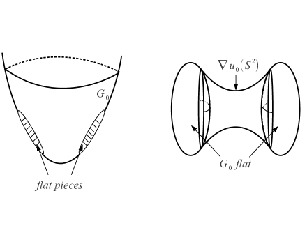
Figure 8. G0subscript๐บ0G_{0} is linear on two bounded convex sets containing โˆ‡u0โ€‹({|x1|>r})โˆ‡subscript๐‘ข0subscript๐‘ฅ1๐‘Ÿ\nabla u_{0}(\{|x_{1}|>r\}).

Let G0subscript๐บ0G_{0} be the function on โ„3superscriptโ„3\mathbb{R}^{3} obtained by revolving Hยฏยฏ๐ป\bar{H} around the p1subscript๐‘1p_{1} axis (see figure 8). By construction u0subscript๐‘ข0u_{0} solves the Euler-Lagrange equation divโ€‹(โˆ‡G0โ€‹(โˆ‡u0))=0divโˆ‡subscript๐บ0โˆ‡subscript๐‘ข00\text{div}(\nabla G_{0}(\nabla u_{0}))=0 away from the cone C0={|x1|=r}subscript๐ถ0subscript๐‘ฅ1๐‘ŸC_{0}=\{|x_{1}|=r\} where r=x22+x33๐‘Ÿsuperscriptsubscript๐‘ฅ22superscriptsubscript๐‘ฅ33r=\sqrt{x_{2}^{2}+x_{3}^{3}}. Thus, it is not immediate that u0subscript๐‘ข0u_{0} minimizes โˆซB1G0โ€‹(โˆ‡u0)โ€‹๐‘‘xsubscriptsubscript๐ต1subscript๐บ0โˆ‡subscript๐‘ข0differential-d๐‘ฅ\int_{B_{1}}G_{0}(\nabla u_{0})\,dx. However, we claim u0subscript๐‘ข0u_{0} is a minimizer. To show this we must establish

โˆซB1โˆ‡G0โ€‹(โˆ‡u0)โ‹…โˆ‡ฯˆโ€‹dโ€‹x=0subscriptsubscript๐ต1โ‹…โˆ‡subscript๐บ0โˆ‡subscript๐‘ข0โˆ‡๐œ“๐‘‘๐‘ฅ0\int_{B_{1}}\nabla G_{0}(\nabla u_{0})\cdot\nabla\psi\,dx=0

for any ฯˆโˆˆC0โˆžโ€‹(B1)๐œ“subscriptsuperscript๐ถ0subscript๐ต1\psi\in C^{\infty}_{0}(B_{1}). The contribution from integrating in Bฯตsubscript๐ตitalic-ฯตB_{\epsilon} and a thin cone {(1โˆ’ฯต)โ€‹r<|x1|<(1+ฯต)โ€‹r}1italic-ฯต๐‘Ÿsubscript๐‘ฅ11italic-ฯต๐‘Ÿ\{(1-\epsilon)r<|x_{1}|<(1+\epsilon)r\} is small. Integrating by parts in the remaining region with boundary S๐‘†S, we get a boundary term of the form โˆซSฯˆโ€‹โˆ‡G0โ€‹(โˆ‡u0)โ‹…ฮฝโ€‹๐‘‘ssubscript๐‘†โ‹…๐œ“โˆ‡subscript๐บ0โˆ‡subscript๐‘ข0๐œˆdifferential-d๐‘ \int_{S}\psi\nabla G_{0}(\nabla u_{0})\cdot\nu\,ds where ฮฝ๐œˆ\nu is the outer normal. The cones {|x1|=(1ยฑฯต)โ€‹r}subscript๐‘ฅ1plus-or-minus1italic-ฯต๐‘Ÿ\{|x_{1}|=(1\pm\epsilon)r\} are ฯตitalic-ฯต\epsilon close, and the outward normals on these cones are ฯตitalic-ฯต\epsilon close to flipping direction, so by the continuity of โˆ‡G0โˆ‡subscript๐บ0\nabla G_{0} the contribution from this term is also small. Taking ฯตitalic-ฯต\epsilon to zero we get the desired result.

Acknowledgement

C. Mooney was supported by NSF fellowship DGE 1144155.

O. Savin was supported by NSF grant DMS-1200701.

References

  • [AS] Ambrosio, L.; Soner, H. M. Level set approach to mean curvature flow in arbitrary codimension. J. Differential Geom. 43 (1996), 693-737.
  • [CF] Colombo, M.; Figalli, A. Regularity results for very degenerate elliptic equations. J. Math. Pures Appl. (9) 101 (2014), no. 1, 94-117.
  • [DG1] De Giorgi, E. Sulla differenziabilitร  e lโ€™analicitร  delle estremali degli integrali multipli regolari. Mem. Accad. Sci. Torino cl. Sci. Fis. Fat. Nat. 3 (1957), 25-43.
  • [DG2] De Giorgi, I. Un esempio di estremali discontinue per un problema variazionale di tipo ellittico. Boll. UMI 4 (1968), 135-137.
  • [DS] De Silva, D.; Savin O. Minimizers of convex functionals arising in random surfaces. Duke Math. J. 151, no. 3 (2010), 487-532.
  • [E1] Evans, L. C. A new proof of local C1,ฮฑsuperscript๐ถ1๐›ผC^{1,\alpha} regularity for solutions of certain degenerate elliptic p.d.e. J. Differential Equations 45 (1982), no. 3, 356-373.
  • [E2] Evans, L. C. Quasiconvexity and partial regularity in the calculus of variations. Arch. Rational Mech. Anal. 95 (1986), no. 3, 227-252.
  • [Gi] Giaquinta, M. Multiple integrals in the calculus of variations and nonlinear elliptic systems. Princeton University Press, Princeton, 1983.
  • [GG] Giaquinta, M.; Giusti, E. Nonlinear elliptic systems with quadratic growth. Manu. Math. 24 (1978), 323-349.
  • [GM1] Giusti, E.; Miranda, M. Sulla regolaritร  delle soluzioni deboli di una classe di sistemi ellittici quasi-lineari. Arch. Rational Mech. Anal. 31 (1968), 173-184.
  • [GM2] Giusti, E.; Miranda, M. Un esempio di soluzione discontinua per un problem di minimo relativo ad un integrale regolare del calcolo delle variazioni. Boll. Un. Mat. Ital. 2 (1968), 1-8.
  • [HLN] Hao, W.; Leonardi, S.; Neฤas, J. An example of an irregular solution to a nonlinear Euler-Lagrange elliptic system with real analytic coefficients. Ann. Scuola Norm. Sup. Pisa Cl. Sci. (4) 23 (1996), no. 1, 57-67.
  • [Mo] Morrey, C. B. Multiple Integrals in the Calculus of Variations. Springer-Verlag, Heidelberg, NY (1966).
  • [Na] Nash, J. Continuity of solutions of parabolic and elliptic equations. Amer. J. Math. 80 (1958), 931-954.
  • [Ne] Neฤas, J. Example of an irregular solution to a nonlinear elliptic system with analytic coefficients and conditions of regularity. Theory of Non Linear Operators, Abhandlungen Akad. der Wissen. der DDR (1997), Proc. of a Summer School held in Berlin (1975).
  • [SY1] ล verรกk, V.; Yan, X. A singular minimizer of a smooth strongly convex functional in three dimensions. Cal. Var. PDE 10 (2000), no.3, 213-221.
  • [SY2] ล verรกk, V.; Yan, X. Non-Lipschitz minimizers of smooth uniformly convex functionals. Proc. Natl. Acad. Sci. USA 99 (2002), no. 24, 15269-15276.