Two samples test for discrete power-law distributions
Abstract
Power-law distributions occur in wide variety of physical, biological, and social phenomena. In this paper, we propose a statistical hypothesis test based on the log-likelihood ratio to assess whether two samples of discrete data are drawn from the same power-law distribution.
keywords:
1 Introduction
Power-law distributions have attracted particular attention for their mathematical properties and appearances in a wide variety of scientific contexts, from physical and biological sciences to social and man-made phenomena.
Differently from those Normally distributed, empirical quantities distributed according to a power-law do not cluster around an average value, and thus we can not characterize a power-law distribution through its mean and standard deviation. However, the fact that some scientific observations can not be characterized as simply as other measurements is often a sign of complex underlying processes that deserve further study [1].
Formally, a discrete or continuous quantity is distributed according to a power-law if its probability distribution is
where is called the scaling parameter of the distribution. However, only few empirical phenomena show such a probability distribution for all values of . More often, the power-law applies only for values greater than some minimum value , so that only the tail of a distribution behaves according to a power-law.
A complete introduction to power-law distributions along with a statistical framework for discerning and quantifying power-law behavior in empirical data can be found in [1], whereas extensive discussions can be found in [2, 3, 4], and references therein.
In this paper, we limit our attention to discrete power-law distributions. In particular, we focus on the comparison of two samples of discrete data to assess whether they are drawn from the same power-law distribution. For example, we could be interested in assessing whether the number of likes received by posts on Facebook and the number of likes received by videos on YouTube follow the same power-law distribution, or whether the degrees of the nodes belonging to two separate clusters in a small-world network are distributed according to the same power-law distribution. To answer those questions we can not rely on the Kolmogorov-Smirov test [5, 6]. Since such a statistical test is formulated for continuous distributions, its application to discrete distributions will produce approximate p-values due to the presence of ties.
In order to overcome such an issue, we introduce a statistical hypothesis test based on the log-likelihood ratio to assess whether two samples of discrete data are drawn from the same population. Under the null hypothesis, i.e. the two samples are drawn from the same power-law distribution, the resulting test statistics follows the distribution with degree of freedom.
This paper is structured as follows. In Section 2 we provide some basic definitions about discrete power-law distributions. In Section 3 we first introduce and discuss the proposed statistical test, and then we conclude with two examples illustrating how the test performs.
2 Definitions
Discrete power-law distributions.
Power-law distributions can be continuous or discrete. Here we focus on the discrete case, i.e. when the quantity of interest can assume only positive integers. Let represents the quantity whose distribution we are interested in. The probability distribution is
where
is the generalized or Hurwitz zeta function. It is useful to consider also the complementary cumulative distribution function,
since it allows to plot power-law distributions in doubly logarithmic axes, and thus emphasize the upper tail behavior.
Estimating the scaling parameter.
The method for fitting parametrized models to observed data is the method of maximum likelihood, which provably gives accurate parameter estimates in the limit of large sample size [7, 8]. The likelihood function of a power-law distribution given a sample is
whereas the log-likelihood function is
Assuming that data are drawn from a power-law distribution with , we can derive a maximum likelihood estimators (MLE) of the scaling parameter . Although there is no exact closed form expression for the MLE in the discrete case, an approximate expression can be derived using an approach that considers power-law distributed integers approximated as continuous reals rounded to the nearest integer (details of the derivation are given in Appendix B of [1]). The result is
3 Two samples test for discrete power-law distributions
Statistical hypothesis test.
Suppose that we have two samples of discrete data, and , and we want to assess whether the two samples are drawn from the same power-law distribution. We can not rely on the Kolmogorov-Smirnov test. Indeed, since such a statistical test is formulated for continuous distributions, its application to discrete distributions will produce approximate p-values due to the presence of ties. In order to overcome such an issue, we propose a statistical test based on the log-likelihood ratio:
where , i.e. the null model, is the log-likelihood of the pooled samples, , whereas , i.e. the alternative model, is the sum of the log-likelihoods of the samples and .
Under the null hypothesis, i.e. the two samples are drawn from the same power-law distribution, the obtained test statistics will follow a distribution with degree of freedom. Indeed, , since in the alternative hypothesis we need to estimate two parameters, and , whereas in the null model we need to estimate only one parameter .
Example 1: two samples drawn from the same distribution.
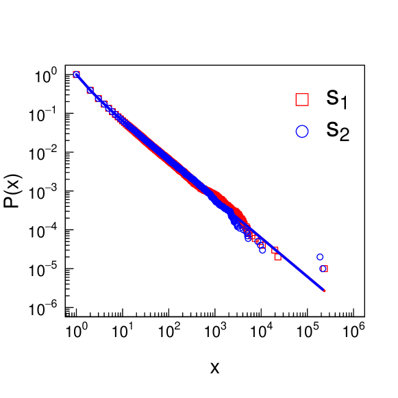
Figure 1 shows the complementary cumulative distribution function, , of two samples, () and (), that we want to compare in order to assess whether they are drawn from the same power-law distribution. The estimates of the scaling parameters are, respectively, and . The test statistics is with p-value , thus we fail to reject the null hypothesis and conclude that the two samples are drawn from the same power-law distribution. Indeed, these samples were randomly drawn from a power-law distribution with and .

Example 2: two samples drawn from different distributions.
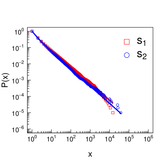
Figure 2 shows the complementary cumulative distribution function, , of two samples, () and (), that we want to compare in order to assess whether they are drawn from the same power-law distribution. The estimates of the scaling parameters are, respectively, and . The test statistics is with p-value , thus we reject the null hypothesis and conclude that the two samples are not drawn from the same power-law distribution. Indeed, these samples were randomly drawn from two power-law distributions with different scaling parameters, respectively, and , with .

References
- [1] Aaron Clauset and Cosma Rohilla Shalizi and M. E. J. Newman (2009). Power-Law Distributions in Empirical Data, SIAM Review, 51(4), pp 661-703, http://dx.doi.org/10.1137/070710111
- [2] Mitzenmacher, M. (2004), Internet Mathematics 1, 226
- [3] Newman, M. E. J. (2005), Contemporary Physics 46, 323
- [4] Sornette, D. (2006), Critical Phenomena in Natural Sciences, Springer, Berlin, chapter 14, 2nd edition.
- [5] William J. Conover (1971), Practical Nonparametric Statistics. New York: John Wiley & Sons. Pages 295-301 (one-sample Kolmogorov test), 309-314 (two-sample Smirnov test).
- [6] George Marsaglia, Wai Wan Tsang and Jingbo Wang (2003), Evaluating Kolmogorov’s distribution. Journal of Statistical Software, 8/18
- [7] Barndorff-Nielsen, O. E., and D. R. Cox (1995). Inference and Asymptotics, Chapman and Hall, London.
- [8] Wasserman, L. (2003). All of Statistics: A concise Course in Statistical Inference, Springer-Verlag, Berlin.