Abstract

We present a flavour-covariant formalism for scalar triplet leptogenesis, which takes into account the effects of the different lepton flavours in a consistent way. Our main finding is that flavour effects can never be neglected in scalar triplet leptogenesis, even in the temperature regime where all charged lepton Yukawa interactions are out of equilibrium. This is at variance with the standard leptogenesis scenario with heavy Majorana neutrinos. In particular, the so-called single flavour approximation leads to predictions for the baryon asymmetry of the universe that can differ by a large amount from the flavour-covariant computation in all temperature regimes. We investigate numerically the impact of flavour effects and spectator processes on the generated baryon asymmetry, and find that the region of triplet parameter space allowed by successsful leptogenesis is significantly enlarged.

1 Introduction

Leptogenesis [1], i.e. the generation of a lepton asymmetry through the out-of-equilibrium decays of heavy particles before sphaleron freeze-out, is one of the most appealing explanations for the origin of the observed baryon asymmetry of the universe. As such, it has been the subject of a large number of studies, especially in its minimal version involving heavy right-handed neutrinos (for a comprehensive review, see Ref. [2]). Over the years, many refinements have been added to the computation of the generated baryon asymmetry: spectator processes [3, 4], finite temperature corrections [5], lepton flavour effects [6, 7, 8, 9, 10] and finally attempts to provide a full quantum mechanical formulation of thermal leptogenesis [11, 12, 13, 14, 15, 16, 17, 18].

By constrast, much less work has been devoted to the leptogenesis scenarios involving fermionic [19, 20, 21, 22, 23] or scalar [24, 25, 26, 27, 28, 29, 30, 31] electroweak triplets (for a recent review of these scenarios and additional references, see Refs. [32]). The CP asymmetry in scalar triplet/antitriplet decays was computed for various models in Refs [24, 25]. A detailed quantitative study of scalar triplet leptogenesis was performed in the single flavour approximation in Ref. [26], and was extended to the supersymmetric case in Ref. [27]. Flavour effects were addressed in flavour non-covariant approaches in Refs. [30, 31], and spectator processes were also included in Ref. [31]. In this paper, we extend and improve previous works on flavour-dependent scalar triplet leptogenesis by providing a complete set of flavour-covariant Boltzmann equations using the density matrix formalism [33, 6]. We find that flavour covariance is a crucial ingredient of the computation of the generated baryon asymmetry, and that flavour effects also matter in the temperature regime where charged lepton Yukawa interactions are out of equilibrium. We show in particular that, as opposed to the standard leptogenesis scenario with right-handed neutrinos, the single flavour calculation does not provide a good approximation to the full flavoured computation, even when charged lepton Yukawa couplings can be neglected.

The paper is organized as follows. The framework and the basic ingredients of flavour-dependent scalar triplet leptogenesis are presented in Section 2. In Section 3, we justify the use of a flavour-covariant formalism and derive the Boltzmann equation for the density matrix in the closed time path formalism. Spectator processes and chemical equilibrium are discussed in Section 4. Section 5 provides the set of Boltzmann equations relevant to the different temperature regimes, both in the flavour-covariant approach with spectator processes included, and in various approximations neglecting flavour covariance and/or spectator processes. In Section 6, we study numerically the impact of flavour effects and spectator processes on scalar triplet leptogenesis, and we compare the flavour-covariant with the flavour non-covariant computations. We find that the generated baryon asymmetry can be significantly enhanced (up to several orders of magnitude) by the proper inclusion of flavour effects and spectator processes, thus enlarging the region of triplet parameter space allowed by successsful leptogenesis. Finally, we present our conclusions in Section 7. The formulae for the space-time densities of reactions used in the paper can be found in Appendix A.

2 Basic ingredients of scalar triplet leptogenesis

2.1 The framework

We work in the framework of the type II seesaw model [34], i.e. the Standard Model augmented with a massive scalar electroweak triplet which couples to left-handed leptons and to the Higgs boson as follows:

$$\mathcal{L}\,=\,-\frac{1}{2}\left(f_{\alpha\beta}\ell_{\alpha}^{T}Ci\sigma^{2}\Delta\ell_{\beta}+\mu H^{T}i\sigma^{2}\Delta^{\dagger}H+\mbox{h.c.}\right)-M_{\Delta}^{2}\,\mbox{tr}(\Delta^{\dagger}\Delta)\,,$$ (2.1)

where $C$ is the charge conjugation matrix defined by $C\gamma^{T}_{\mu}C^{-1}=-\gamma_{\mu}$, and

$$\Delta\,=\,\left(\begin{array}[]{cc}\Delta^{+}/\sqrt{2}&\Delta^{++}\\ \Delta^{0}&-\Delta^{+}/\sqrt{2}\end{array}\right),\qquad\Delta^{\dagger}\,=\,\left(\begin{array}[]{cc}\Delta^{-}/\sqrt{2}&\Delta^{0*}\\ \Delta^{--}&-\Delta^{-}/\sqrt{2}\end{array}\right).$$ (2.6)

When decomposed on the components of each electroweak multiplet, this Lagrangian becomes

$$\mathcal{L}\,=\,- \frac{1}{2}\left\{f_{\alpha\beta}\left(\nu_{\alpha}^{T}C\nu_{\beta}\,\Delta^{0}-\sqrt{2}\,\nu_{\alpha}^{T}Ce_{\beta}\,\Delta^{+}-e_{\alpha}^{T}Ce_{\beta}\,\Delta^{++}\right)\right.$$

$$+ \left.\mu\left(-H^{0}H^{0}\Delta^{0*}-\sqrt{2}\,H^{0}H^{+}\Delta^{-}+H^{+}H^{+}\Delta^{--}\right)+\mbox{h.c.}\right\}$$

$$-\, M_{\Delta}^{2}\left(\Delta^{0*}\Delta^{0}+\Delta^{-}\Delta^{+}+\Delta^{--}\Delta^{++}\right).$$ (2.7)

The triplet gives a contribution to the neutrino mass matrix:

$$(m_{\Delta})_{\alpha\beta}\,=\,\frac{1}{2}\,\mu f_{\alpha\beta}\frac{v^{2}}{M_{\Delta}^{2}}\,,$$ (2.8)

where $v=\langle H^{0}\rangle=174\,\mathrm{GeV}$ is the Higgs boson vacuum expectation value. In addition to generating small neutrino masses, the heavy scalar triplet can also create a lepton asymmetry through its decays, like the right-handed neutrinos of the type I seesaw mechanism. There are however important differences between the standard leptogenesis scenario involving heavy Majorana neutrinos and scalar triplet leptogenesis. First $\Delta$ has 2 types of decays, into Higgs bosons and into antileptons, with tree-level decay rates

$$\Gamma(\Delta\rightarrow\bar{\ell}\bar{\ell})\,=\,\frac{1}{32\pi}\,\mathrm{tr}(ff^{\dagger})M_{\Delta}\,,\qquad\Gamma(\Delta\rightarrow HH)\,=\,\frac{1}{32\pi}\,\frac{|\mu|^{2}}{M_{\Delta}}\,.$$ (2.9)

It will prove convenient in the following to introduce the quantities:

$$\lambda_{\ell}\,\equiv\,\sqrt{\text{tr}(ff^{\dagger})}\,,\qquad\qquad\lambda_{H}\,\equiv\,\frac{|\mu|}{M_{\Delta}}\,,$$ (2.10)

which control the tree-level decay width and branching ratios of the scalar triplet:

$$\Gamma_{\Delta}\,=\,\frac{1}{32\pi}\left(\lambda^{2}_{\ell}+\lambda^{2}_{H}\right)M_{\Delta}\,,$$ (2.11)

$$B_{\ell}\,\equiv\,\mathrm{BR}(\Delta\rightarrow\bar{\ell}\bar{\ell})\,=\,\frac{\lambda_{\ell}^{2}}{\lambda_{\ell}^{2}+\lambda_{H}^{2}}\ ,\qquad B_{H}\,\equiv\,\mathrm{BR}(\Delta\rightarrow HH)\,=\,\frac{\lambda_{H}^{2}}{\lambda_{\ell}^{2}+\lambda_{H}^{2}}\ .$$ (2.12)

Second, in contrast to the heavy Majorana neutrinos of standard leptogenesis, the scalar triplet is not a self-conjugate state. Hence, an asymmetry between the triplet and antitriplet abundances will arise and affect the dynamics of leptogenesis. Third, being charged under $SU(2)_{L}\times U(1)_{Y}$, the triplets and antitriplets can annihilate before decaying. In order to generate a large enough lepton asymmetry, decays have to happen with a rate higher or similar to gauge annihilations, which are typically in thermal equilibrium. This requirement seems to conflict with Sakharov’s third condition [35], but the fact that the triplet has several decay channels makes it possible for some of them to occur out of equilibrium and resolves the contradiction [26].

Finally, another important feature of scalar triplet leptogenesis, whose significance has been missed so far, lies in the fact that the scalar triplet couples to pairs of leptons from different generations rather than to a coherent superposition of lepton flavours (as opposed to a right-handed neutrino). As a consequence, its dynamics cannot be described by Boltzmann equations involving a single lepton asymmetry. This is at variance with the standard leptogenesis scenario, in which neglecting the effects of the different lepton flavours is a good approximation at high temperature. For scalar triplet leptogenesis, a flavour-covariant formalism must be employed, as will be discussed in Section 3.

In order for leptogenesis to account for the observed baryon asymmetry of the universe, a large enough asymmetry between the leptonic decay rates of triplets and antitriplets is needed. It is a well-known fact [36, 37] that this condition is not satisfied with the minimal particle content of the type II seesaw mechanism, since there is no CP asymmetry in $\Delta$/$\bar{\Delta}$ decays at the one-loop level. For this to happen, another heavy state (or possibly several heavy states) with couplings to the lepton and Higgs doublets must be added to the model. If this additional particle is significantly heavier than $\Delta$, it will not be present in the thermal bath at the time of leptogenesis and its effect can be parametrized by the effective dimension-5 operator [26]

$$\Delta\mathcal{L}_{\rm eff}\,=\,\frac{1}{4}\,\frac{\kappa_{\alpha\beta}}{\Lambda}\,(\ell^{T}_{\alpha}i\sigma^{2}H)\,C\,(H^{T}i\sigma^{2}\ell_{\beta})+\mbox{h.c.}\,,$$ (2.13)

suppressed by $\Lambda\gg M_{\Delta}$, where $\Lambda=M^{2}_{\Delta^{\prime}}/\mu^{\prime}=M_{\Delta^{\prime}}/\lambda^{\prime}_{H}$ if the heavier particle is a scalar triplet $\Delta^{\prime}$, and $\Lambda=M$ if it is a right-handed neutrino or a fermionic triplet with mass $M$. The operator (2.13) also gives a contribution to the neutrino mass matrix:

$$(m_{\mathcal{H}})_{\alpha\beta}=\frac{1}{2}\kappa_{\alpha\beta}\frac{v^{2}}{\Lambda}\,.$$ (2.14)

In full generality one should also add an effective dimension-6 operator (which arises at tree level if the heavier particle is a scalar triplet [30], but only at the one-loop level if it is a right-handed neutrino or a fermionic triplet):

$$\Delta^{\prime}\mathcal{L}_{\rm eff}\,\,=\,-\frac{1}{4}\,\frac{\eta_{\alpha\beta\gamma\delta}}{\Lambda^{2}}\left(\ell_{\alpha}^{T}Ci\sigma^{2}\vec{\sigma}\ell_{\beta}\right)\!\cdot\!\left(\bar{\ell}_{\gamma}\vec{\sigma}i\sigma^{2}C\bar{\ell}_{\delta}^{T}\right),$$ (2.15)

where $\eta_{\alpha\beta\gamma\delta}$ is symmetric under the exchanges $\alpha\leftrightarrow\beta$ and $\gamma\leftrightarrow\delta$. This operator induces a contribution to the flavour-dependent CP asymmetries in $\Delta$/$\bar{\Delta}$ decays that vanishes when summed over lepton flavours, hence it only affects leptogenesis when the dynamics of the different flavours is taken into account. However, it generally plays a subdominant role because it is suppressed by an additional power of $\Lambda$ (and possibly also by a loop factor) with respect to the operator (2.13). A notable exception arises when (2.13) and (2.15) are generated by a heavier scalar triplet $\Delta^{\prime}$ with couplings to lepton and Higgs doublets such that $\lambda_{H}\lambda^{\prime}_{H}\ll\lambda_{\ell}\lambda^{\prime}_{\ell}M_{\Delta}/M_{\Delta^{\prime}}$. In this case, the operator (2.15) gives the dominant contribution to the flavour-dependent CP asymmetries in $\Delta$ decays, while the total CP asymmetry (to which only (2.13) contributes) is small. This scenario, dubbed purely flavoured leptogenesis (PFL) in the literature, has been studied in Refs. [30, 31]. In this paper we shall stick to the less specific case of dominance of the operator (2.13) and omit the operator (2.15).

2.2 CP Asymmetries in $\Delta$/$\bar{\Delta}$ decays

Figure 1: Diagrams responsible for the flavour-dependent CP asymmetries $\epsilon_{\alpha\beta}$.

The CP asymmetries in the decays of the triplets and antitriplets are defined by

$$\epsilon_{H}\,\equiv\,2\ \frac{\Gamma(\Delta\rightarrow HH)-\Gamma(\bar{\Delta}\rightarrow\bar{H}\bar{H})}{\Gamma_{\Delta}+\Gamma_{\bar{\Delta}}}\,,$$ (2.16)

$$\epsilon_{\alpha\beta}\,\equiv\,\frac{\Gamma(\bar{\Delta}\rightarrow\ell_{\alpha}\ell_{\beta})-\Gamma(\Delta\rightarrow\bar{\ell}_{\alpha}\bar{\ell}_{\beta})}{\Gamma_{\Delta}+\Gamma_{\bar{\Delta}}}\ \left(1+\delta_{\alpha\beta}\right),$$ (2.17)

where we included a factor 2 in the definitions of $\epsilon_{H}$ and $\epsilon_{\alpha\alpha}$ for later convenience. The flavour-dependent CP asymmetries $\epsilon_{\alpha\beta}$ come from the interference between the diagrams shown in Fig. 1. With the definition (2.17), they can be expressed in terms of $m_{\Delta}$ and $m_{\cal H}$ as

$$\epsilon_{\alpha\beta}\,=\,\frac{1}{4\pi}\frac{M_{\Delta}}{v^{2}}\sqrt{B_{\ell}B_{H}}\ \frac{\mbox{Im}\left[(m^{*}_{\Delta})_{\alpha\beta}(m_{\mathcal{H}})_{\alpha\beta}\right]}{\bar{m}_{\Delta}}\,,$$ (2.18)

where we have introduced

$$\bar{m}_{\Delta}\,\equiv\,\sqrt{\text{tr}(m_{\Delta}^{\dagger}m_{\Delta})}\,.$$ (2.19)

The total CP asymmetry is given by [26]

$$\epsilon_{\Delta}\,\equiv\,\sum_{\alpha,\beta}\epsilon_{\alpha\beta}\,=\,\frac{1}{4\pi}\frac{M_{\Delta}}{v^{2}}\sqrt{B_{\ell}B_{H}}\ \frac{\mbox{Im}\left[\mbox{tr}(m^{\dagger}_{\Delta}m_{\mathcal{H}})\right]}{\bar{m}_{\Delta}}\,=\,\epsilon_{H}\,,$$ (2.20)

where the last equality follows from CPT invariance.

2.3 Washout processes

The lepton asymmetry generated in triplet and antitriplet decays is partially washed out by lepton number violating processes. These include the inverse decays $\ell_{\alpha}\ell_{\beta}\rightarrow\bar{\Delta}$ and $\bar{\ell}_{\alpha}\bar{\ell}_{\beta}\rightarrow\Delta$, and the $\Delta L=2$ scatterings $\ell_{\alpha}\ell_{\beta}\leftrightarrow\bar{H}\bar{H}$ and $\ell_{\alpha}H\leftrightarrow\bar{\ell}_{\beta}\bar{H}$, mediated by $s$- and $t$-channel triplet exchange, respectively, as well as by the higher order operator (2.13). In addition, some processes that preserve total lepton number redistribute the asymmetries between the different lepton flavours, namely the 2 lepton–2 lepton scatterings $\ell_{\alpha}\ell_{\beta}\leftrightarrow\ell_{\gamma}\ell_{\delta}$ and $\ell_{\alpha}\bar{\ell}_{\gamma}\leftrightarrow\bar{\ell}_{\beta}\ell_{\delta}$ (mediated by s- and t-channel triplet exchange, respectively), and the 2–2 scatterings involving leptons and triplets $\ell_{\alpha}\Delta\leftrightarrow\ell_{\beta}\Delta$, $\ell_{\alpha}\bar{\Delta}\leftrightarrow\ell_{\beta}\bar{\Delta}$ and $\ell_{\alpha}\bar{\ell}_{\beta}\leftrightarrow\Delta\bar{\Delta}$ (mediated by s-, t- and u-channel lepton exchange). Since the asymmetries stored in different lepton flavours are subject to different washout rates, these flavour violating processes have an impact on the erasure of the total lepton number, and we will refer to them as washout processes, too.

We define for later reference the space-time density of triplet and antitriplet decays:

$$\gamma_{D}\,=\,\sum_{\alpha,\beta}\left[\gamma(\Delta\leftrightarrow\bar{\ell}_{\alpha}\bar{\ell}_{\beta})+\gamma(\bar{\Delta}\leftrightarrow\ell_{\alpha}\ell_{\beta})\right]+\gamma(\Delta\leftrightarrow HH)+\gamma(\bar{\Delta}\leftrightarrow\bar{H}\bar{H})\,,$$ (2.21)

as well as the following combinations of flavour-dependent scattering densities:

$$\gamma_{\ell H}\, =\,\sum_{\alpha,\beta}\left[2\gamma(\ell_{\alpha}\ell_{\beta}\leftrightarrow\bar{H}\bar{H})+\gamma(\ell_{\alpha}H\leftrightarrow\bar{\ell}_{\beta}\bar{H})\right],$$ (2.22)

$$\gamma_{4\ell}\, =\,\sum_{\alpha,\beta,\gamma,\delta}\left[2\gamma(\ell_{\alpha}\ell_{\beta}\leftrightarrow\ell_{\gamma}\ell_{\delta})+\gamma(\ell_{\alpha}\bar{\ell}_{\gamma}\leftrightarrow\bar{\ell}_{\beta}\ell_{\delta})\right],$$ (2.23)

$$\gamma_{\ell\Delta}\, =\,\sum_{\alpha,\beta}\left[\gamma(\ell_{\alpha}\Delta\leftrightarrow\ell_{\beta}\Delta)+\gamma(\ell_{\alpha}\bar{\Delta}\leftrightarrow\ell_{\beta}\bar{\Delta})+\gamma(\ell_{\alpha}\bar{\ell}_{\beta}\leftrightarrow\Delta\bar{\Delta})\right].$$ (2.24)

3 Flavour-covariant formalism

3.1 The need for a flavour-covariant formalism

Leptogenesis computations are often performed in the so-called single flavour approximation, in which a single direction in flavour space is considered. This is a rather accurate approximation in scenarios in which a heavy Majorana neutrino $N_{1}$ decaying at high temperature is responsible for the whole lepton asymmetry. Indeed, the couplings of $N_{1}$ can be rewritten as (with the contraction of $SU(2)_{L}$ indices omitted)

$$-\sum_{\alpha}Y_{1\alpha}\bar{N}_{1}\ell_{\alpha}H+\mbox{h.c.}\,=\,-y\bar{N}_{1}\ell_{N_{1}\,}\!H+\mbox{h.c.}\,,$$ (3.1)

where $y\equiv\sqrt{\sum_{\alpha}|Y_{1\alpha}|^{2}}$ and $\ell_{N_{1}}\equiv\sum_{\alpha}Y_{1\alpha}\ell_{\alpha}/y$. When processes mediated by the charged lepton Yukawa couplings are out of equilibrium, i.e. when $N_{1}$ decays in the high temperature regime ($T>10^{12}\,\mathrm{GeV}$), the coherence of $\ell_{N_{1}}$ is effectively preserved by all interactions in the thermal plasma and leptogenesis can safely be described in terms of a single lepton flavour. When the lepton asymmetry is generated at lower temperature, on the other hand, charged lepton Yukawa interactions enter equilibrium and destroy the coherence of $\ell_{N_{1}}$. The single flavour approximation is no longer appropriate, and the proper treatment involves a $3\times 3$ matrix in lepton flavour space [6], the density matrix $(\Delta_{\ell})_{\alpha\beta}$, whose diagonal entries are the asymmetries stored in each lepton doublet $\ell_{\alpha}$, while the off-diagonal entries encode the quantum correlations between the different flavours. This matrix transforms as $\Delta_{\ell}\to U^{*}\Delta_{\ell}\,U^{T}$ under flavour rotations $\ell\to U\ell$, and its evolution is governed by a flavour-covariant Boltzmann equation.

However, in the case of leptogenesis with right-handed neutrinos discussed above, the density matrix formalism is only really needed at the transition between two temperature regimes [42], or in the case where several heavy Majorana neutrinos contribute to the generation and washout of the lepton asymmetry as in Refs. [6, 43, 44, 38], or in resonant leptogenesis [45, 39]. Otherwise there is always a natural choice of basis in which the Boltzmann equation for $(\Delta_{\ell})_{\alpha\beta}$ can be substituted for a set of Boltzmann equations for 1, 2 or 3 flavour asymmetries. Above $T=10^{12}\,\mathrm{GeV}$, where all charged lepton Yukawa couplings are out of equilibrium, the appropriate flavour basis is $(\ell_{N_{1}},\ell_{\perp 1},\ell_{\perp 2})$, where $\ell_{\perp 1}$ and $\ell_{\perp 2}$ are two directions in flavour space perpendicular to $\ell_{N_{1}}$. In this basis, leptogenesis is well described in terms of the sole lepton asymmetry $\Delta_{\ell_{N_{1}}}$. Below $T=10^{12}\,\mathrm{GeV}$, tau Yukawa-induced processes like $q_{3}\ell_{\tau}\to t_{R}\tau_{R}$ are in equilibrium and destroy the coherence between $\ell_{\tau}$ and the other two lepton flavours. However, as long as the muon Yukawa coupling is out of equilibrium (which is the case if $T>10^{9}\,\mathrm{GeV}$), the coherence of $\ell_{0}\equiv(Y_{1e}\ell_{e}+Y_{1\mu}\ell_{\mu})/\sqrt{|Y_{1e}|^{2}+|Y_{1\mu}|^{2}}$ is preserved, and the dynamics of leptogenesis can be described in a 2-flavour approximation, in terms of the asymmetries $\Delta_{\ell_{0}}$ and $\Delta_{\ell_{\tau}}$. Finally, below $T=10^{9}\,\mathrm{GeV}$, the muon Yukawa interactions are in equilibrium as well, and flavour coherence is completely broken. Leptogenesis is then governed by Boltzmann equations for the three asymmetries $\Delta_{\ell_{e}}$, $\Delta_{\ell_{\mu}}$ and $\Delta_{\ell_{\tau}}$.

The case of scalar triplet leptogenesis is significantly different, because the scalar triplet does not couple to a single combination of lepton flavours in general. This makes the use of a flavour-covariant formalism unavoidable as long as the quantum correlations between lepton flavours are not destroyed by charged lepton Yukawa interactions. One can still define formally a single flavour approximation by making the substitutions $(\Delta_{\ell})_{\alpha\beta}\to\Delta_{\ell}$, $f_{\alpha\beta}\to\lambda_{\ell}$, $\kappa_{\alpha\beta}\to\lambda_{\kappa}\equiv\sqrt{\mbox{tr}(\kappa\kappa^{\dagger})}$ and $\mathcal{E}_{\alpha\beta}\to\epsilon_{\Delta}$ (where $\mathcal{E}_{\alpha\beta}$ are the flavour-covariant CP asymmetries, to be defined later), but the resulting Boltzmann equations cannot be derived from the flavour-covariant ones by taking the limit of vanishing Yukawa couplings. Hence, even if the scalar triplets decay above $T=10^{12}\,\mathrm{GeV}$, there is no guarantee that the single flavour calculation will give a good approximation to the flavour-covariant result.

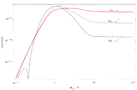
Figure 2: The $B-L$ asymmetry generated in scalar triplet leptogenesis as a function of $z=m_{\Delta}/T$, computed following three different prescriptions: density matrix computation using the Boltzmann equations (5.1)–(5.3), yielding $\Delta_{B-L}=\text{tr}(\Delta_{\alpha\beta})$ (red solid curve); naive computation using the Boltzmann equations (5.8)–(5.10) written in the charged lepton mass eigenstate basis, yielding $(\Delta_{B-L})^{1}=\Delta_{e}+\Delta_{\mu}+\Delta_{\tau}$ (black dashed curve); naive computation performed in the neutrino mass eigenstate basis, yielding $(\Delta_{B-L})^{2}=\Delta_{1}+\Delta_{2}+\Delta_{3}$ (black dotted curve). The parameters are $M_{\Delta}=10^{13}\,\mathrm{GeV}$, $\lambda_{H}=0.01$ and, in the notation of Eqs. (6.3) and (6.4), $\phi_{12}=\phi_{13}=\pi/4$, $\phi_{23}=0$, $\beta_{1}=\pi/4$ and $\beta_{2}=\pi/6$, all other phases being zero.

A less naive approach is to neglect flavour covariance but keep track of the different lepton flavours, and write classical Boltzmann equations for the three asymmetries $\Delta_{\ell_{\alpha}}$. When the lepton asymmetry is generated below $T=10^{9}\,\mathrm{GeV}$, this is fully justified because quantum correlations between the different lepton flavours are destroyed by fast interactions induced by the muon and tau Yukawa couplings. In this case, the appropriate flavour basis is the charged lepton mass eigenstate basis: $\Delta_{\ell_{\alpha}}=\{\Delta_{\ell_{e}},\Delta_{\ell_{\mu}},\Delta_{\ell_{\tau}}\}$. When all charged lepton Yukawa interactions are out of equilibrium, however, the choice of the flavour basis becomes a delicate issue. In fact, it turns out that Boltzmann equations written in different bases cannot be transformed into one another by a flavour rotation $\ell\to U\ell$, and give different numerical results for the baryon asymmetry. This is illustrated in Fig. 2, which compares the $B-L$ asymmetry computed in the flavour-covariant formalism using the density matrix with the naive computation involving Boltzmann equations for the flavour asymmetries $\Delta_{\ell_{\alpha}}$, written either in the charged lepton or in the neutrino mass eigenstate basis. Since physics should not depend on a choice of basis, we are led to conclude that the density matrix formalism is the only valid approach when charged lepton Yukawa interactions are out of equilibrium.

In the intermediate temperature range where the tau Yukawa coupling is in equilibrium but the muon and electron Yukawa couplings are not, the quantum correlations between the tau and the other flavours are destroyed. In practice, this means that the off-diagonal entries in the third line and the third column of the density matrix are driven to zero by the fast tau Yukawa interactions. Thus, the relevant dynamical variables in this regime are the $2\times 2$ density matrix $(\Delta^{0}_{\ell})_{\alpha\beta}$ describing the asymmetries stored in the lepton doublets $\ell_{e}$, $\ell_{\mu}$ and their quantum correlations, and the asymmetry $\Delta_{\ell_{\tau}}$ stored in $\ell_{\tau}$.

3.2 The Boltzmann equation for the density matrix

The derivation of the evolution equation for the density matrix is not straightforward. In this paper, we shall use the closed time path (CTP) formalism [46], which has been used to obtain flavoured quantum Boltzmann equations for the standard leptogenesis scenario with heavy Majorana neutrinos [11, 12, 13, 14, 15, 16, 17, 18] (for other approaches, also in the framework of the standard leptogenesis scenario, see e.g. Refs. [8, 42] or the review [2]). In this formalism, which is well adapted to describe non-equilibrium phenomena in quantum field theory, particle densities are replaced by Green’s functions defined on a closed path $\mathcal{C}$ in the complex time plane going from an initial instant $t=0$ to $t=+\infty$ and back. When applied to leptogenesis, this formalism leads to quantum Boltzmann equations involving memory effects and off-shell corrections [11]; in particular, the CP asymmetries are functions of time and their values depend on the history of the system. Such effects can be important for resonant leptogenesis and soft leptogenesis [12, 47], but they are not expected to play a significant role in the scenario studied in this paper, which does not involve degenerate states. We shall therefore ignore them and make several simplifying assumptions in order to obtain a (classical) flavour-covariant Boltzmann equation for the density matrix. In particular, we shall ignore plasma/thermal effects and apply the CTP formalism to quantum field theory at zero temperature. This procedure is going to provide us with an equation of the form:

$$sHz\frac{d(\Delta_{\ell})_{\alpha\beta}}{dz}\,=\,\left(\frac{\Sigma_{\Delta}}{\Sigma_{\Delta}^{\text{eq}}}-1\right)\!\gamma_{D}\,\mathcal{E}_{\alpha\beta}-\mathcal{W}^{D}_{\alpha\beta}-\mathcal{W}^{\ell H}_{\alpha\beta}-\mathcal{W}^{4\ell}_{\alpha\beta}-\mathcal{W}^{\ell\Delta}_{\alpha\beta}\,,$$ (3.2)

where the right-hand side contains a source term proportional to the flavour-covariant CP-asymmetry matrix $\mathcal{E}_{\alpha\beta}$ and washout terms associated with inverse triplet and antitriplet decays ($\mathcal{W}^{D}_{\alpha\beta}$), $2\to 2$ scatterings involving leptons and Higgs bosons ($\mathcal{W}^{\ell H}_{\alpha\beta}$), 2 lepton–2 lepton scatterings ($\mathcal{W}^{4\ell}_{\alpha\beta}$) and $2\to 2$ scatterings involving leptons and triplets ($\mathcal{W}^{\ell\Delta}_{\alpha\beta}$). By construction, Eq. (3.2) is covariant under flavour rotations $\ell\to U\ell$, which means that each of the matrices $\mathcal{E}$, $\mathcal{W}^{D}$, $\mathcal{W}^{\ell H}$, $\mathcal{W}^{4\ell}$, $\mathcal{W}^{\ell\Delta}$ transforms in the same way as the density matrix $\Delta_{\ell}$, namely as $\mathcal{M}\to U^{*}\mathcal{M}U^{T}$.

Before proceeding with the derivation of Eq. (3.2), let us specify our notations. For any species $X=\ell_{\alpha},H,\Delta$, we define the comoving number density $Y_{X}\equiv n_{X}/s$, where $s$ is the entropy density, and the asymmetry stored in $X$ by $\Delta_{X}\equiv Y_{X}-Y_{\bar{X}}=(n_{X}-n_{\bar{X}})/s$. We also define the comoving number density of triplets and antitriplets $\Sigma_{\Delta}\equiv(n_{\Delta}+n_{\bar{\Delta}})/s$. The evolution of these quantities as a function of $z\equiv M_{\Delta}/T$ is governed by a set of Boltzmann equations. Finally, a superscript ^eq denotes an equilibrium density.

3.2.1 Derivation of the Boltzmann equation in the CTP formalism

The relevant degrees of freedom in scalar triplet leptogenesis are lepton doublets, Higgs doublets and scalar triplets. We will therefore need the following Green’s functions, coresponding to all possible orderings of the fields along the closed time path $\mathcal{C}$ (for a review of the CTP formalism, see Ref. [48]):

$$G_{\alpha\beta}^{>}(x,y)\, =\,-i\langle\ell_{\alpha}(x)\bar{\ell}_{\beta}(y)\rangle\,,$$ (3.3)

$$G_{\alpha\beta}^{<}(x,y)\, =\,i\langle\bar{\ell}_{\beta}(y)\ell_{\alpha}(x)\rangle\,,$$ (3.4)

$$G_{\alpha\beta}^{t}(x,y)\, =\,\theta(x^{0}-y^{0})G_{\alpha\beta}^{>}(x,y)+\theta(y^{0}-x^{0})G_{\alpha\beta}^{<}(x,y)\,,$$ (3.5)

$$G_{\alpha\beta}^{\bar{t}}(x,y)\, =\,\theta(y^{0}-x^{0})G_{\alpha\beta}^{>}(x,y)+\theta(x^{0}-y^{0})G_{\alpha\beta}^{<}(x,y)\,,$$ (3.6)

where $\alpha,\beta$ are lepton flavour indices, and the $\ell$’s refer to left-handed lepton doublets, whereas for a scalar field $\phi(x)$ (representing a Higgs doublet or a scalar triplet):

$$G_{\phi}^{>}(x,y)\, =\,-i\langle\phi(x)\phi^{\dagger}(y)\rangle\,,$$ (3.7)

$$G_{\phi}^{<}(x,y)\, =\,-i\langle\phi^{\dagger}(y)\phi(x)\rangle\,,$$ (3.8)

$$G_{\phi}^{t}(x,y)\, =\,\theta(x^{0}-y^{0})G_{\phi}^{>}(x,y)+\theta(y^{0}-x^{0})G_{\phi}^{<}(x,y)\,,$$ (3.9)

$$G_{\phi}^{\bar{t}}(x,y)\, =\,\theta(y^{0}-x^{0})G_{\phi}^{>}(x,y)+\theta(x^{0}-y^{0})G_{\phi}^{<}(x,y)\,.$$ (3.10)

The brackets $\langle...\rangle$ mean that we take the average over all available states of the system. One can write these Green’s functions as a single $2\times 2$ matrix:

$$\tilde{G}_{\mathbin{\mathchoice{\ooalign{\raisebox{0.6pt}{\small{$\displaystyle B$}}\cr\smash{\raisebox{-0.6pt}{\small{$\displaystyle F$}}}\cr}}{\ooalign{\raisebox{0.6pt}{\small{$\textstyle B$}}\cr\smash{\raisebox{-0.6pt}{\small{$\textstyle F$}}}\cr}}{\ooalign{\raisebox{0.6pt}{\small{$\scriptstyle B$}}\cr\smash{\raisebox{-0.6pt}{\small{$\scriptstyle F$}}}\cr}}{\ooalign{\raisebox{0.6pt}{\small{$\scriptscriptstyle B$}}\cr\smash{\raisebox{-0.6pt}{\small{$\scriptscriptstyle F$}}}\cr}}}}\,=\left(\begin{matrix}G^{t}&\pm G^{<}\\ G^{>}&-G^{\bar{t}}\end{matrix}\right),$$ (3.11)

where the plus sign refers to bosons and the minus sign to fermions. This matrix satisfies the following Schwinger-Dyson equation:

$$\tilde{G}(x,y)\,=\,\tilde{G}^{0}(x,y)+\int_{\mathcal{C}}d^{4}w_{1}\int_{\mathcal{C}}d^{4}w_{2}\,\tilde{G}^{0}(x,w_{1})\tilde{\Sigma}(w_{1},w_{2})\tilde{G}(w_{2},y)\,,$$ (3.12)

where $\tilde{\Sigma}$ is a $2\times 2$ matrix containing the self-energy functions $\Sigma^{>}$, $\Sigma^{<}$, $\Sigma^{t}$ and $\Sigma^{\bar{t}}$, defined in an analogous way to the Green’s functions $G^{>}$, $G^{<}$, $G^{t}$ and $G^{\bar{t}}$:

$$\tilde{\Sigma}_{\mathbin{\mathchoice{\ooalign{\raisebox{0.6pt}{\small{$\displaystyle B$}}\cr\smash{\raisebox{-0.6pt}{\small{$\displaystyle F$}}}\cr}}{\ooalign{\raisebox{0.6pt}{\small{$\textstyle B$}}\cr\smash{\raisebox{-0.6pt}{\small{$\textstyle F$}}}\cr}}{\ooalign{\raisebox{0.6pt}{\small{$\scriptstyle B$}}\cr\smash{\raisebox{-0.6pt}{\small{$\scriptstyle F$}}}\cr}}{\ooalign{\raisebox{0.6pt}{\small{$\scriptscriptstyle B$}}\cr\smash{\raisebox{-0.6pt}{\small{$\scriptscriptstyle F$}}}\cr}}}}\,=\left(\begin{matrix}\Sigma^{t}&\pm\Sigma^{<}\\ \Sigma^{>}&-\Sigma^{\bar{t}}\end{matrix}\right),$$ (3.21)

and $\tilde{G}^{0}$ is the free 2-point correlation function. The Schwinger-Dyson equation can also be written as

$$\tilde{G}(x,y)\,=\,\tilde{G}^{0}(x,y)+\int_{\mathcal{C}}d^{4}w_{1}\int_{\mathcal{C}}d^{4}w_{2}\,\tilde{G}(x,w_{1})\tilde{\Sigma}(w_{1},w_{2})\tilde{G}^{0}(w_{2},y)\,.$$ (3.22)

In the fermionic case, we note for later use that acting on Eqs. (3.12) and (3.22) with the operators $i\!\overrightarrow{\not{\partial}}_{\!x}$ and $i\!\overleftarrow{\not{\partial}}_{\!y}$, respectively, gives the following equations of motion:

$$i\!\overrightarrow{\not{\partial}}_{\!x}\tilde{G}_{\alpha\beta}(x,y)\, =\,\delta^{(4)}(x-y)\,\delta_{\alpha\beta}\,\tilde{I}\,+\,\sum_{\gamma}\int_{\mathcal{C}}d^{4}w\,\tilde{\Sigma}_{\alpha\gamma}(x,w)\tilde{G}_{\gamma\beta}(w,y)\,,$$ (3.23)

$$\tilde{G}_{\alpha\beta}(x,y)\,i\!\overleftarrow{\not{\partial}}_{\!y}\, =\,-\,\delta^{(4)}(x-y)\,\delta_{\alpha\beta}\,\tilde{I}\,+\,\sum_{\gamma}\int_{\mathcal{C}}d^{4}w\,\tilde{G}_{\alpha\gamma}(x,w)\tilde{\Sigma}_{\gamma\beta}(w,y)\,,$$ (3.24)

where we have restored the flavour indices and used the fact that the free Green’s function for massless fermions satisfies $i\not{\partial}_{x}\tilde{G}_{\alpha\beta}^{0}(x,y)=\delta^{(4)}(x-y)\,\delta_{\alpha\beta}\,\tilde{I}$, with $\tilde{I}$ the identity matrix in both spinor and CTP spaces.

Writing the free Dirac field as

$$\psi(x)\,=\,\int\frac{d^{3}\vec{p}}{(2\pi)^{3}\sqrt{2\omega_{\vec{p}}}}\sum_{s}\left(u(p,s)b(\vec{p},s)e^{-ip\cdot x}+v(p,s)d^{\dagger}(\vec{p},s)e^{ip\cdot x}\right),$$ (3.25)

where $\omega_{\vec{p}}=\sqrt{{\vec{p}}^{\;2}+m^{2}}$, we define the phase-space distribution functions of lepton and antilepton doublets $\rho_{\alpha\beta}(\vec{p})$ and $\bar{\rho}_{\alpha\beta}(\vec{p})$ as matrices in flavour space by

$$\langle b_{\alpha}^{\dagger}(\vec{p})b_{\beta}(\vec{p^{\prime}})\rangle\,=\,(2\pi)^{3}\delta^{(3)}(\vec{p}-\vec{p^{\prime}})\rho_{\alpha\beta}(\vec{p})\,,$$ (3.26)

$$\langle d_{\beta}^{\dagger}(\vec{p})d_{\alpha}(\vec{p^{\prime}})\rangle\,=\,(2\pi)^{3}\delta^{(3)}(\vec{p}-\vec{p^{\prime}})\bar{\rho}_{\alpha\beta}(\vec{p})\,.$$ (3.27)

The reversed order of the flavour indices $\alpha$ and $\beta$ in the definition of $\bar{\rho}_{\alpha\beta}(\vec{p})$ ensures that the distribution functions of lepton and antilepton doublets transform in the same way under a rotation in flavour space, $\ell\to U\ell\,$:

$$\rho\ \rightarrow\ U^{*}\rho\,U^{T},$$ (3.28)

$$\bar{\rho}\ \rightarrow\ U^{*}\bar{\rho}\,U^{T}.$$ (3.29)

Similarly, the phase-space distribution functions of a charged scalar $\phi$ and of its antiparticle are defined by

$$\langle a^{\dagger}_{\phi}(\vec{p})a_{\phi}(\vec{p^{\prime}})\rangle\,=\,(2\pi)^{3}\delta^{(3)}(\vec{p}-\vec{p^{\prime}})\rho_{\phi}(\vec{p})\,,$$ (3.30)

$$\langle b_{\phi}^{\dagger}(\vec{p})b_{\phi}(\vec{p^{\prime}})\rangle\,=\,(2\pi)^{3}\delta^{(3)}(\vec{p}-\vec{p^{\prime}})\bar{\rho}_{\phi}(\vec{p})\,,$$ (3.31)

where $a_{\phi}(\vec{p})$ and $b_{\phi}^{\dagger}(\vec{p})$ are the annihilation and creation operators appearing in the definition of the free charged scalar field:

$$\phi(x)\,=\,\int\frac{d^{3}\vec{p}}{(2\pi)^{3}\sqrt{2\omega_{\vec{p}}}}\left(a_{\phi}(\vec{p})e^{-ip\cdot x}+b_{\phi}^{\dagger}(\vec{p})e^{ip\cdot x}\right).$$ (3.32)

With these definitions, the Green’s functions for left-handed lepton doublets can be written as (neglecting lepton masses)

$$iG_{\alpha\beta}^{>}(x,y)\, =\,P_{L}\int\frac{d^{3}p}{(2\pi)^{3}2\omega_{\vec{p}}}\ \,\not{p}\left\{[\delta_{\alpha\beta}-\rho_{\beta\alpha}(\vec{p})]\,e^{-ip\cdot(x-y)}+\bar{\rho}_{\beta\alpha}(\vec{p})\,e^{ip\cdot(x-y)}\right\}P_{R}\,,$$ (3.33)

$$iG_{\alpha\beta}^{<}(x,y)\, =\,-P_{L}\int\frac{d^{3}p}{(2\pi)^{3}2\omega_{\vec{p}}}\ \,\not{p}\left\{\rho_{\beta\alpha}(\vec{p})\,e^{-ip\cdot(x-y)}+[\delta_{\alpha\beta}-\bar{\rho}_{\beta\alpha}(\vec{p})]\,e^{ip\cdot(x-y)}\right\}P_{R}\,,$$ (3.34)

whereas for scalars one obtains

$$iG_{\phi}^{>}(x,y)\,=\,\int\frac{d^{3}p}{(2\pi)^{3}2\omega_{\vec{p}}}\left\{[1+\rho_{\phi}(\vec{p})]\,e^{-ip\cdot(x-y)}+\bar{\rho}_{\phi}(\vec{p})\,e^{ip\cdot(x-y)}\right\}\,,$$ (3.35)

$$iG_{\phi}^{<}(x,y)\,=\,\int\frac{d^{3}p}{(2\pi)^{3}2\omega_{\vec{p}}}\left\{\rho_{\phi}(\vec{p})\,e^{-ip\cdot(x-y)}+[1+\bar{\rho}_{\phi}(\vec{p})]\,e^{ip\cdot(x-y)}\right\}\,.$$ (3.36)

Strictly speaking, these expressions are valid for free Green’s functions only, but they will be sufficient for our purpose. Notice that, under charge conjugation,

$$\mathcal{C}G_{\alpha\beta}^{>}\mathcal{C}^{-1}(x,y)\, =\,CG_{\beta\alpha}^{<T}(y,x)C^{-1}\,\equiv\,-G_{\beta\alpha_{R}}^{<}(y,x)\,,$$ (3.37)

$$\mathcal{C}G_{\phi}^{>}\mathcal{C}^{-1}(x,y)\, =\,G_{\phi}^{<}(y,x)\,,$$ (3.38)

where $C$, not to be confused with the charge conjugation operator $\mathcal{C}$, is the charge conjugation matrix defined by $C\gamma^{T}_{\mu}C^{-1}=-\gamma_{\mu}$, and the quantity $G_{\beta\alpha_{R}}^{<}$ in Eq. (3.37) is defined as $G_{\beta\alpha}^{<}$ in Eq. (3.34) with $P_{L}$ interchanged with $P_{R}$.

The comoving number densities of scalars and left-handed leptons, and of their antiparticles, are given by

$$Y_{\phi}\,\equiv\,\frac{n_{\phi}}{s}\,=\,\frac{g_{\phi}}{s}\int\frac{d^{3}p}{(2\pi)^{3}}\,\rho_{\phi}(\vec{p})\,,\qquad Y_{\alpha\beta}\,\equiv\,\frac{n_{\alpha\beta}}{s}\,=\,\frac{2}{s}\int\frac{d^{3}p}{(2\pi)^{3}}\,\rho_{\alpha\beta}(\vec{p})\,,$$ (3.39)

$$Y_{\bar{\phi}}\,\equiv\,\frac{n_{\bar{\phi}}}{s}\,=\,\frac{g_{\phi}}{s}\int\frac{d^{3}p}{(2\pi)^{3}}\,\bar{\rho}_{\phi}(\vec{p})\,,\qquad\bar{Y}_{\alpha\beta}\,\equiv\,\frac{\bar{n}_{\alpha\beta}}{s}\,=\,\frac{2}{s}\int\frac{d^{3}p}{(2\pi)^{3}}\,\bar{\rho}_{\alpha\beta}(\vec{p})\,,$$ (3.40)

where $Y_{\alpha\beta}$ and $\bar{Y}_{\alpha\beta}$, similarly to the phase-space distribution functions $\rho_{\alpha\beta}(\vec{p})$ and $\bar{\rho}_{\alpha\beta}(\vec{p})$, are matrices in flavour space, and $g_{\phi}=2$ (resp. $g_{\phi}=3$) for Higgs bosons (resp. scalar triplets). One also defines the matrix of lepton asymmetries (hereafter called “density matrix”):

$$(\Delta_{\ell})_{\alpha\beta}\,\equiv\,\frac{\Delta n_{\alpha\beta}}{s}\,=\,Y_{\alpha\beta}-\bar{Y}_{\alpha\beta}\,.$$ (3.41)

The diagonal entries of $(\Delta_{\ell})_{\alpha\beta}$ correspond to the flavour asymmetries stored in lepton doublets, while the off-diagonal entries encode the quantum correlations between the different flavour asymmetries. From the definition (3.41) and from Eqs. (3.28) and (3.29) one can see that $\Delta_{\ell}$ transforms under a rotation in flavour space $\ell\to U\ell$ as

$$\Delta_{\ell}\,\to\,U^{*}\Delta_{\ell}\,U^{T}.$$ (3.42)

One can show that $\Delta n_{\alpha\beta}$ is the zeroth component of the current $J_{\alpha\beta}^{\mu}=\,:\!\bar{\ell}_{\alpha}\gamma^{\mu}\ell_{\beta}\!:$ (or more precisely of its average $\langle J_{\alpha\beta}^{\mu}\rangle$):

$$\Delta n_{\alpha\beta}\,=\,\langle J_{\alpha\beta}^{0}\rangle\,=\,\langle\,:\!\ell^{\dagger}_{\alpha}\ell_{\beta}\!:\,\rangle\,.$$ (3.43)

We will use this fact to derive an evolution equation for $\Delta n_{\alpha\beta}$. Noticing that

$$\langle\partial_{\mu}J_{\alpha\beta}^{\mu}\rangle\,=\, -\mathrm{tr}\left[(i\!\overrightarrow{\not{\partial}}_{\!x}+i\!\overleftarrow{\not{\partial}}_{\!y})G_{\beta\alpha}^{>}(x,y)\right]_{y\,=\,x}\ ,$$ (3.44)

where the trace is taken over spinorial and $SU(2)_{L}$ indices, and using the Schwinger-Dyson equations (3.23) and (3.24) to express the right-hand side of Eq. (3.44) in terms of the self-energy functions $\Sigma^{>}$ and $\Sigma^{<}$, one obtains

$$\langle\partial_{\mu}J_{\alpha\beta}^{\mu}\rangle\,=\, -\int_{\mathcal{C}}d^{4}w\ \mathrm{tr}\left[\Sigma_{\beta\gamma}^{>}(x,w)G_{\gamma\alpha}^{t}(w,x)-\Sigma_{\beta\gamma}^{\bar{t}}(x,w)G_{\gamma\alpha}^{>}(w,x)\right.$$

$$\left.-G_{\beta\gamma}^{>}(x,w)\Sigma_{\gamma\alpha}^{t}(w,x)+G_{\beta\gamma}^{\bar{t}}(x,w)\Sigma_{\gamma\alpha}^{>}(w,x)\right]$$

$$=\, -\int d^{3}w\int_{0}^{t}dt_{w}\ \mathrm{tr}\left[\Sigma_{\beta\gamma}^{>}(x,w)G_{\gamma\alpha}^{<}(w,x)-\Sigma_{\beta\gamma}^{<}(x,w)G_{\gamma\alpha}^{>}(w,x)\right.$$

$$\left.-G_{\beta\gamma}^{>}(x,w)\Sigma_{\gamma\alpha}^{<}(w,x)+G_{\beta\gamma}^{<}(x,w)\Sigma_{\gamma\alpha}^{>}(w,x)\right].$$ (3.45)

Since we consider a homogeneous and isotropic medium, the divergence of the current reduces to $d\Delta n_{\alpha\beta}/dt$. Finally, we incorporate the expansion of the universe by making the following replacement in the above equation:

$$\langle\partial_{\mu}J_{\alpha\beta}^{\mu}\rangle\ \ \rightarrow\ \ \frac{d\Delta n_{\alpha\beta}}{dt}+3H\Delta n_{\alpha\beta}\,=\,sHz\frac{d(\Delta_{\ell})_{\alpha\beta}}{dz}\ .$$ (3.46)

We thus obtain the quantum Boltzmann equation for the density matrix $(\Delta_{\ell})_{\alpha\beta}$:

$$sHz\frac{d(\Delta_{\ell})_{\alpha\beta}}{dz}\,=\, -\int d^{3}w\int_{0}^{t}dt_{w}\ \mathrm{tr}\left[\Sigma_{\beta\gamma}^{>}(x,w)G_{\gamma\alpha}^{<}(w,x)-\Sigma_{\beta\gamma}^{<}(x,w)G_{\gamma\alpha}^{>}(w,x)\right.$$

$$\left.-G_{\beta\gamma}^{>}(x,w)\Sigma_{\gamma\alpha}^{<}(w,x)+G_{\beta\gamma}^{<}(x,w)\Sigma_{\gamma\alpha}^{>}(w,x)\right].$$ (3.47)

This equation is both quantum and flavour-covariant, but we are only interested in flavour effects. We shall therefore take the classical limit by keeping only the contributions to $\Sigma$ involving an on-shell intermediate part. This procedure will provide us with a flavour-covariant Boltzmann equation of the form (3.2).

3.2.2 Washout terms: decays and inverse decays

Let us first compute the flavour-covariant washout term $W^{D}_{\alpha\beta}$ associated with triplet/antitriplet decays and inverse decays. In the CTP formalism, this term arises from the 1-loop contribution to the lepton doublet self-energy shown in Fig. 3. For the first term of the integrand on the right-hand side of Eq. (3.47), this gives

Figure 3: 1-loop contribution to the lepton doublet self-energy $\Sigma_{\beta\alpha}(x,y)$.

$$\mathrm{tr}\!\left[\Sigma_{\beta\gamma}^{>}(x,w)G_{\gamma\alpha}^{<}(w,x)\right]\,=\ \, (-if_{\beta\rho}^{*})(-if_{\gamma\sigma})\,\mathrm{tr}\Big{[}iG_{\Delta}^{<}(w,x)(-i)G_{\sigma\rho_{R}}^{<}(w,x)iG_{\gamma\alpha}^{<}(w,x)\Big{]}$$

$$=\ \, 3\int\frac{d^{3}p}{(2\pi)^{3}2\omega_{\vec{p}}}\int\frac{d^{3}k}{(2\pi)^{3}2\omega_{\vec{k}}}\int\frac{d^{3}l}{(2\pi)^{3}2\omega_{\vec{\ell}}}\ f_{\beta\rho}^{*}f_{\gamma\sigma}\,2(k.l)\,$$

$$\times\left\{\rho_{\Delta}(\vec{p})\,e^{-ip\cdot(w-x)}+[1+\bar{\rho}_{\Delta}(\vec{p})]\,e^{ip\cdot(w-x)}\right\}$$

$$\times\left\{\rho_{\rho\sigma}(\vec{k})\,e^{-ik\cdot(w-x)}+[\delta_{\rho\sigma}-\bar{\rho}_{\rho\sigma}(\vec{k})]\,e^{ik\cdot(w-x)}\right\}$$

$$\times\left\{\rho_{\alpha\gamma}(\vec{l})\,e^{-il\cdot(w-x)}+[\delta_{\alpha\gamma}-\bar{\rho}_{\alpha\gamma}(\vec{l})]\,e^{il\cdot(w-x)}\right\},$$ (3.48)

where the factor 3 comes from the trace over $SU(2)_{L}$ indices. The integration over the spatial coordinates of $w$ gives a momentum-conserving delta function. In the integral over $t_{w}$, we take the classical limit by making the usual assumption that $t$ is much smaller than the relaxation time of particle distributions, which can therefore be factorized out of the integral, but much larger than the typical duration of a collision, so that the time integral can be extended to infinity. This amounts to replacing the integral of oscillating exponentials by energy-conserving delta functions, plus terms proportional to the principal values of $1/(\omega_{\vec{p}}\pm\omega_{\vec{k}}\pm\omega_{\vec{l}})$, where $p$, $k$ and $l$ are the momenta of the scalar triplet and of the two leptons, respectively. The latter terms, however, can be neglected because they arise at second order in the CP asymmetry. Indeed, all terms involving a principal value are proportional to $\eta_{\rho\sigma}(\vec{k})+\bar{\eta}_{\rho\sigma}(\vec{k})$, where $\eta_{\rho\sigma}(\vec{k})$ (resp. $\bar{\eta}_{\rho\sigma}(\vec{k})$) parametrizes the departure of the phase-space density $\rho_{\rho\sigma}(\vec{k})$ (resp. $\bar{\rho}_{\rho\sigma}(\vec{k})$) from its equilibrium value:

$$\rho_{\rho\sigma}(\vec{k})\,=\,\rho_{\ell}^{\text{eq}}(\vec{k})\left[\delta_{\rho\sigma}+\eta_{\rho\sigma}(\vec{k})\right],\quad\bar{\rho}_{\rho\sigma}(\vec{k})\,=\,\rho_{\ell}^{\text{eq}}(\vec{k})\left[\delta_{\rho\sigma}+\bar{\eta}_{\rho\sigma}(\vec{k})\right].$$ (3.49)

Since the unbalance between the lepton and antilepton densities is generated by the asymmetries in triplet decays, which are small numbers of order $\epsilon$, while the lepton and antilepton populations are maintained close to equilibrium by fast electroweak interactions, one has

$$\eta_{\rho\sigma}(\vec{k})-\bar{\eta}_{\sigma\rho}(\vec{k})\, =\,\mathcal{O}(\epsilon)\,,$$ (3.50)

$$\eta_{\rho\sigma}(\vec{k})+\bar{\eta}_{\sigma\rho}(\vec{k})\, =\,\mathcal{O}(\epsilon^{2})\,.$$ (3.51)

Therefore, the terms proportional to $\eta_{\rho\sigma}(\vec{k})+\bar{\eta}_{\rho\sigma}(\vec{k})$ on the right-hand side of the Boltzmann equation (3.47) are of order $\epsilon^{2}$ and can safely be neglected. By doing so one keeps only the terms that are kinematically allowed for on-shell particles. Dropping Bose enhancement and Pauli blocking factors, we obtain

$$- \int d^{3}w\int_{0}^{\infty}dt_{w}\ \mathrm{tr}\!\left[\Sigma_{\beta\gamma}^{>}(x,w)G_{\gamma\alpha}^{<}(w,x)\right]$$

$$= -\int\frac{d^{3}p}{(2\pi)^{3}2\omega_{\vec{p}}}\int\frac{d^{3}k}{(2\pi)^{3}2\omega_{\vec{k}}}\int\frac{d^{3}l}{(2\pi)^{3}2\omega_{\vec{\ell}}}\ 3f_{\beta\rho}^{*}f_{\gamma\sigma}(k.l)\,(2\pi)^{4}\delta^{(4)}(p-k-l)$$

$$\times\left\{\rho_{\rho\sigma}(\vec{k})\rho_{\alpha\gamma}(\vec{\ell})+\rho_{\Delta}(\vec{p})\delta_{\rho\sigma}\delta_{\alpha\gamma}\right\}.$$ (3.52)

Proceeding in the same way to compute the other contributions from Fig. 3 to the right-hand side of the Boltwmann equation (3.47), and introducing the space-time density of triplet and antitriplet decays:

$$\gamma_{D}\,=\, \int\frac{d^{3}p}{(2\pi)^{3}2\omega_{\vec{p}}}\int\frac{d^{3}k}{(2\pi)^{3}2\omega_{\vec{k}}}\int\frac{d^{3}l}{(2\pi)^{3}2\omega_{\vec{\ell}}}\ 3\left(\lambda_{\ell}^{2}+\lambda_{H}^{2}\right)(k.l)$$

$$\times(2\pi)^{4}\delta^{(4)}(p-k-l)\left\{\rho_{\Delta}^{\mathrm{eq}}(\vec{p})+\bar{\rho}_{\Delta}^{\mathrm{eq}}(\vec{p})\right\},$$ (3.53)

we obtain the washout term $\mathcal{W}^{D}_{\alpha\beta}$ associated with decays and inverse decays:

$$\mathcal{W}^{D}_{\alpha\beta}\,=\,\frac{2B_{\ell}}{\lambda_{\ell}^{2}}\left[(ff^{\dagger})_{\alpha\beta}\frac{\Delta_{\Delta}}{\Sigma_{\Delta}^{\mathrm{eq}}}\ +\frac{1}{4(Y_{\ell}^{\mathrm{eq}})^{2}}\left(YfY^{T}f^{\dagger}+fY^{T}f^{\dagger}Y-Y\leftrightarrow\bar{Y}\right)_{\alpha\beta}\right]\!\gamma_{D}\,,$$ (3.54)

where we remind the reader that $\Delta_{\Delta}\equiv(n_{\Delta}-n_{\bar{\Delta}})/s$ and $\Sigma_{\Delta}\equiv(n_{\Delta}+n_{\bar{\Delta}})/s$. One can linearize this expression using again the fact that flavour-blind gauge interactions keep the lepton densities close to their equilibrium values:

$$Y_{\alpha\beta}-\bar{Y}_{\alpha\beta}\, =\,(\Delta_{\ell})_{\alpha\beta}\,,$$

$$Y_{\alpha\beta}+\bar{Y}_{\alpha\beta}\, =\,2Y_{\ell}^{\mathrm{eq}}\left[\delta_{\alpha\beta}+\mathcal{O}(\epsilon^{2})\right],$$ (3.55)

which finally gives

$$\mathcal{W}^{D}_{\alpha\beta}\,=\,\frac{2B_{\ell}}{\lambda_{\ell}^{2}}\left[(ff^{\dagger})_{\alpha\beta}\frac{\Delta_{\Delta}}{\Sigma_{\Delta}^{\text{eq}}}+\frac{1}{4Y_{\ell}^{\text{eq}}}\left(2f\Delta_{\ell}^{T}f^{\dagger}+ff^{\dagger}\Delta_{\ell}+\Delta_{\ell}ff^{\dagger}\right)_{\alpha\beta}\right]\!\gamma_{D}\,.$$ (3.56)

Note that the washout term (3.56) contains a piece proportional to $\Delta_{\Delta}$, which is due to decays. This term appears on the right-hand side of the Boltzmann equation for the $3\times 3$ density matrix $(\Delta_{\ell})_{\alpha\beta}$, Eq. (3.2). One can easily check that it transforms as $\mathcal{W}^{D}\to U^{*}\mathcal{W}^{D}U^{T}$ under flavour rotations $\ell\to U\ell$, as required by flavour covariance. Below $T=10^{12}\,\mathrm{GeV}$, however, the tau Yukawa coupling is in equilibrium and drives the $(e,\tau)$, $(\mu,\tau)$, $(\tau,e)$ and $(\tau,\mu)$ entries of the density matrix to zero. The relevant dynamical variables in this regime (or more precisely in the temperature range $10^{9}\,\mathrm{GeV}<T<10^{12}\,\mathrm{GeV}$, before the muon Yukawa coupling enters equilibrium) are $\Delta_{\ell_{\tau}}$, the asymmetry stored in $\ell_{\tau}$, and a $2\times 2$ matrix $\Delta_{\ell}^{0}$ describing the flavour asymmetries stored in the lepton doublets $\ell_{e},\ell_{\mu}$ and their quantum correlations. The corresponding washout terms $\tilde{\mathcal{W}}^{D}_{\alpha\beta}$ (where $\alpha$ and $\beta$ label any two orthogonal directions in the ($\ell_{e}$, $\ell_{\mu}$) flavour subspace) and $\tilde{\mathcal{W}}^{D}_{\tau}$ are simply obtained by setting $(\Delta_{\ell})_{\alpha\tau}=(\Delta^{*}_{\ell})_{\tau\alpha}=\Delta_{\ell_{\tau}}\delta_{\alpha\tau}$ in Eq. (3.56), yielding

$$\tilde{\mathcal{W}}^{D}_{\alpha\beta}\,=\, \frac{2B_{\ell}}{\lambda_{\ell}^{2}}\left[(ff^{\dagger})_{\alpha\beta}\frac{\Delta_{\Delta}}{\Sigma_{\Delta}^{\text{eq}}}\right.$$

$$\left.+\,\frac{1}{4Y_{\ell}^{\text{eq}}}\left(2f(\Delta^{0}_{\ell})^{T}f^{\dagger}+ff^{\dagger}\Delta^{0}_{\ell}+\Delta^{0}_{\ell}ff^{\dagger}\right)_{\alpha\beta}+\frac{1}{2Y_{\ell}^{\text{eq}}}\,f_{\alpha\tau}f_{\beta\tau}^{*}\Delta_{\ell_{\tau}}\right]\!\gamma_{D}\,,$$ (3.57)

and

$$\tilde{\mathcal{W}}^{D}_{\tau}\,=\,\frac{2B_{\ell}}{\lambda_{\ell}^{2}}\left[(ff^{\dagger})_{\tau\tau}\frac{\Delta_{\Delta}}{\Sigma_{\Delta}^{\text{eq}}}+\frac{1}{2Y_{\ell}^{\text{eq}}}\left((f(\Delta^{0}_{\ell})^{T}f^{\dagger})_{\tau\tau}+((ff^{\dagger})_{\tau\tau}+|f_{\tau\tau}|^{2})\,\Delta_{\ell_{\tau}}\right)\right]\!\gamma_{D}\,.$$ (3.58)

The resulting Boltzmann equation for $(\Delta^{0}_{\ell})_{\alpha\beta}$ is covariant under flavour rotations in the ($\ell_{e}$, $\ell_{\mu}$) subspace. Finally, below $T=10^{9}\,\mathrm{GeV}$, the muon Yukawa coupling enters equilibrium and drives the $(e,\mu)$ and $(\mu,e)$ entries of the density matrix to zero. The Boltzmann equation (3.2) then reduces to three equations for the flavour asymmetries $\Delta_{\ell_{\alpha}}\equiv(\Delta_{\ell})_{\alpha\alpha}$ ($\alpha=e,\mu,\tau$), with a washout term $\mathcal{W}^{D}_{\alpha}$ given by

$$\mathcal{W}^{D}_{\alpha}\,=\,\frac{2B_{\ell}}{\lambda_{\ell}^{2}}\,\sum_{\beta}\,|f_{\alpha\beta}|^{2}\left[\frac{\Delta_{\Delta}}{\Sigma_{\Delta}^{\text{eq}}}+\frac{\Delta_{\ell_{\alpha}}+\Delta_{\ell_{\beta}}}{2Y_{\ell}^{\text{eq}}}\right]\!\gamma_{D}\,.$$ (3.59)

3.2.3 Other washout terms: $2\to 2$ scatterings

The other washout terms in the Boltzmann equation (3.2) correspond to $2\to 2$ scatterings and arise from 2-loop contributions to the lepton doublet self-energy $\Sigma_{\beta\alpha}$. The term $\mathcal{W}^{\ell H}_{\alpha\beta}$ accounts for the washout of the flavour asymmetries by the $\Delta L=2$ scatterings $\ell_{\gamma}\ell_{\delta}\leftrightarrow\bar{H}\bar{H}$ and $\ell_{\gamma}H\leftrightarrow\bar{\ell}_{\delta}\bar{H}$ and is given by

$$\mathcal{W}^{\ell H}_{\alpha\beta}\,=\ 2\left\{\frac{1}{\lambda^{2}_{\ell}}\left[\frac{\left(2f\Delta_{\ell}^{T}f^{\dagger}+ff^{\dagger}\Delta_{\ell}+\Delta_{\ell}ff^{\dagger}\right)_{\alpha\beta}}{4Y_{\ell}^{\text{eq}}}+\frac{\Delta_{H}}{Y_{H}^{\text{eq}}}(ff^{\dagger})_{\alpha\beta}\right]\right.\!\gamma_{\ell H}^{\Delta}$$

$$+\frac{1}{\mbox{Re}\left[\text{tr}(f\kappa^{\dagger})\right]}\left[\frac{\left(2f\Delta_{\ell}^{T}\kappa^{\dagger}+f\kappa^{\dagger}\Delta_{\ell}+\Delta_{\ell}f\kappa^{\dagger}\right)_{\alpha\beta}}{4Y_{\ell}^{\text{eq}}}+\frac{\Delta_{H}}{Y_{H}^{\text{eq}}}(f\kappa^{\dagger})_{\alpha\beta}\right]\!\gamma_{\ell H}^{\mathcal{I}}$$

$$+\frac{1}{\mbox{Re}\left[\text{tr}(f\kappa^{\dagger})\right]}\left[\frac{\left(2\kappa\Delta_{\ell}^{T}f^{\dagger}+\kappa f^{\dagger}\Delta_{\ell}+\Delta_{\ell}\kappa f^{\dagger}\right)_{\alpha\beta}}{4Y_{\ell}^{\text{eq}}}+\frac{\Delta_{H}}{Y_{H}^{\text{eq}}}(\kappa f^{\dagger})_{\alpha\beta}\right]\!\gamma_{\ell H}^{\mathcal{I}}$$

$$\left.+\frac{1}{\lambda^{2}_{\kappa}}\left[\frac{\left(2\kappa\Delta_{\ell}^{T}\kappa^{\dagger}+\kappa\kappa^{\dagger}\Delta_{\ell}+\Delta_{\ell}\kappa\kappa^{\dagger}\right)_{\alpha\beta}}{4Y_{\ell}^{\text{eq}}}+\frac{\Delta_{H}}{Y_{H}^{\text{eq}}}(\kappa\kappa^{\dagger})_{\alpha\beta}\right]\!\gamma_{\ell H}^{\mathcal{H}}\right\},$$ (3.60)

where $\Delta_{H}\equiv(n_{H}-n_{\bar{H}})/s$ is the asymmetry stored in the Higgs doublet, $\lambda_{\kappa}\equiv\sqrt{\text{tr}(\kappa\kappa^{\dagger})}$ and $\gamma_{\ell H}^{\Delta}$, $\gamma_{\ell H}^{\mathcal{H}}$ and $\gamma_{\ell H}^{\mathcal{I}}$ are the contributions (summed over lepton flavours) of different self-energy diagrams to the space-time density of $\Delta L=2$ scatterings $\gamma_{\ell H}$. Namely, one has $\gamma_{\ell H}=\gamma_{\ell H}^{\Delta}+2\gamma_{\ell H}^{\mathcal{I}}+\gamma_{\ell H}^{\mathcal{H}}$, in which $\gamma_{\ell H}^{\Delta}$ is the contribution of scalar triplet exchange, $\gamma_{\ell H}^{\mathcal{H}}$ is the contribution of the $D=5$ operator (2.13) responsible for $m_{\mathcal{H}}$, and $2\gamma_{\ell H}^{\mathcal{I}}$ is the interference term. Explicit expressions for the reduced cross-sections that are needed to compute numerically these reaction densities (as well as the ones appearing in Eqs. (3.61) and (3.62) below) can be found in Appendix A.

The washout term due to the 2 lepton–2 lepton scatterings $\ell_{\gamma}\ell_{\delta}\leftrightarrow\ell_{\rho}\ell_{\sigma}$ and $\ell_{\gamma}\bar{\ell}_{\rho}\leftrightarrow\bar{\ell}_{\delta}\ell_{\sigma}$ reads

$$\mathcal{W}^{4\ell}_{\alpha\beta}\,=\,\frac{2}{\lambda^{4}_{\ell}} \left[\lambda^{2}_{\ell}\,\frac{\left(2f\Delta_{\ell}^{T}f^{\dagger}+ff^{\dagger}\Delta_{\ell}+\Delta_{\ell}ff^{\dagger}\right)_{\alpha\beta}}{4Y_{\ell}^{\text{eq}}}-\frac{\text{tr}(\Delta_{\ell}ff^{\dagger})}{Y_{\ell}^{\text{eq}}}(ff^{\dagger})_{\alpha\beta}\right]\!\gamma_{4\ell}\,,$$ (3.61)

whereas the washout term associated with the lepton-triplet scatterings $\ell_{\gamma}\Delta\leftrightarrow\ell_{\delta}\Delta$, $\ell_{\gamma}\bar{\Delta}\leftrightarrow\ell_{\delta}\bar{\Delta}$ and $\ell_{\gamma}\bar{\ell}_{\delta}\leftrightarrow\Delta\bar{\Delta}$ is

$$\mathcal{W}^{\ell\Delta}_{\alpha\beta}\,=\,\frac{1}{\text{tr}(ff^{\dagger}ff^{\dagger})}\left[\frac{1}{2Y_{\ell}^{\text{eq}}}\left(ff^{\dagger}ff^{\dagger}\Delta_{\ell}-2ff^{\dagger}\Delta_{\ell}ff^{\dagger}+\Delta_{\ell}ff^{\dagger}ff^{\dagger}\right)_{\alpha\beta}\right]\!\gamma_{\ell\Delta}\,.$$ (3.62)

This completes the derivation of the washout terms appearing on the right-hand side of Eq. (3.2). The expressions of $\mathcal{W}^{\ell H}_{\alpha\beta}$, $\mathcal{W}^{4\ell}_{\alpha\beta}$ and $\mathcal{W}^{\ell\Delta}_{\alpha\beta}$ relevant in the temperature ranges $10^{9}\,\mathrm{GeV}<T<10^{12}\,\mathrm{GeV}$ and $T<10^{9}\,\mathrm{GeV}$ can be obtained from Eqs. (3.60), (3.61) and (3.62) following the same procedure as the one used for $\mathcal{W}^{D}_{\alpha\beta}$, see the discussion above Eqs. (3.57) and (3.59). Note that $\mathcal{W}^{4\ell}_{\alpha\beta}$ and $\mathcal{W}^{\ell\Delta}_{\alpha\beta}$ vanish in the single flavour approximation where $\alpha$ and $\beta$ take a single value; this is consistent with the fact that the 2 lepton–2 lepton and lepton-triplet scatterings affect leptogenesis only when lepton flavour effects are taken into account.

3.2.4 Source term

Figure 4: 2-loop contributions to the lepton doublet self-energy $\Sigma_{\beta\alpha}$ giving rise to the CP asymmetry $\mathcal{E}_{\alpha\beta}$.

Finally, let us derive the source term of the Boltzmann equation (3.2). In the CTP formalism, the 2-loop self-energy diagrams shown in Fig. 4, when inserted in the right-hand side of Eq. (3.47), give rise to the flavour-covariant source term

$$\mathcal{S}_{\alpha\beta}\,=\left(\frac{\Sigma_{\Delta}}{\Sigma_{\Delta}^{\mathrm{eq}}}-1\right)\!\gamma_{D}\,\mathcal{E}_{\alpha\beta}\,,$$ (3.63)

where $\mathcal{E}_{\alpha\beta}$ is a Hermitian matrix transforming as $\mathcal{E}\to U^{*}\mathcal{E}U^{T}$ under a flavour rotation $\ell\to U\ell$. The explicit form of $\mathcal{E}_{\alpha\beta}$ can be obtained without going through the full CTP computation by noticing that, in the temperature regime $T<10^{9}\,\mathrm{GeV}$ where the quantum correlations among lepton flavours are destroyed by fast interactions induced by the muon and tau Yukawa couplings, the source term for the flavour asymmetry $\Delta_{\ell_{\alpha}}\equiv(\Delta_{\ell})_{\alpha\alpha}$ ($\alpha=e,\mu,\tau$) reads

$$\mathcal{S}_{\alpha\alpha}\,=\,\left(\frac{\Sigma_{\Delta}}{\Sigma_{\Delta}^{\mathrm{eq}}}-1\right)\!\gamma_{D}\sum_{\gamma}\epsilon_{\alpha\gamma}\,,$$ (3.64)

where $\epsilon_{\alpha\gamma}$, not to be confused with $\mathcal{E}_{\alpha\gamma}$, is the CP asymmetry in the decay $\Delta\to\bar{\ell}_{\alpha}\bar{\ell}_{\gamma}$ defined in Eq. (2.17). Comparing Eq. (3.63) with Eq. (3.64) and using Eq. (2.18), one obtains the diagonal entries of $\mathcal{E}$:

$$\mathcal{E}_{\alpha\alpha}\,=\,\sum_{\gamma}\epsilon_{\alpha\gamma}\,=\,\frac{1}{4\pi}\frac{M_{\Delta}}{v^{2}}\sqrt{B_{\ell}B_{H}}\ \frac{\mbox{Im}\left[(m_{\mathcal{H}}\,m_{\Delta}^{\dagger})_{\alpha\alpha}\right]}{\bar{m}_{\Delta}}\ .$$ (3.65)

It is then easy to derive the full flavour-covariant CP-asymmetry matrix $\mathcal{E}$ by reading its dependence on the couplings $f_{\alpha\beta}$ and $\kappa_{\alpha\beta}$ from Fig. 4, and by using its hermiticity and covariance properties together with Eq. (3.65):

$$\mathcal{E}_{\alpha\beta}\,=\,\frac{1}{8\pi i}\frac{M_{\Delta}}{v^{2}}\sqrt{B_{\ell}B_{H}}\ \frac{(m_{\mathcal{H\,}}m_{\Delta}^{\dagger}-m_{\Delta}m_{\mathcal{H}}^{\dagger})_{\alpha\beta}}{\bar{m}_{\Delta}}\,.$$ (3.66)

The first equality in Eq. (3.65) implies that the trace of this matrix is equal to the total CP asymmetry in triplet decays:

$$\mathrm{tr}\,\mathcal{E}\,=\,\sum_{\alpha,\beta}\epsilon_{\alpha\beta}\,=\,\epsilon_{\Delta}\,.$$ (3.67)

This completes the derivation of the right-hand side of the flavour-covariant Boltzmann equation (3.2).

3.3 Full set of Boltzmann equations

Finally, Eq. (3.2) must be supplemented with the Boltzmann equations for $\Sigma_{\Delta}$ and $\Delta_{\Delta}$ (an equation for $\Delta_{H}$ is not needed since, as we are going to see in Section 4, $\Delta_{H}$ can be expressed as a function of the other asymmetries):

$$sHz\frac{d\Sigma_{\Delta}}{dz}\, =\,-\left(\frac{\Sigma_{\Delta}}{\Sigma_{\Delta}^{\text{eq}}}-1\right)\!\gamma_{D}-2\left(\!\left(\frac{\Sigma_{\Delta}}{\Sigma_{\Delta}^{\text{eq}}}\right)^{\!2}-1\right)\!\gamma_{A}\,,$$ (3.68)

$$sHz\frac{d(\Delta_{\ell})_{\alpha\beta}}{dz}\, =\,\left(\frac{\Sigma_{\Delta}}{\Sigma_{\Delta}^{\text{eq}}}-1\right)\!\gamma_{D}\,\mathcal{E}_{\alpha\beta}-\mathcal{W}^{D}_{\alpha\beta}-\mathcal{W}^{\ell H}_{\alpha\beta}-\mathcal{W}^{4\ell}_{\alpha\beta}-\mathcal{W}^{\ell\Delta}_{\alpha\beta}\,,$$ (3.69)

$$sHz\frac{d\Delta_{\Delta}}{dz}\, =\,-\frac{1}{2}\left(\text{tr}(\mathcal{W}^{D})-W^{D}_{H}\right),$$ (3.70)

where the first and second terms in Eq. (3.68) come from (anti)triplet decays and triplet-antitriplet annihilations, respectively, and $W^{D}_{H}$ in Eq. (3.70) is the washout term due to the inverse decays $HH\to\Delta$ and $\bar{H}\bar{H}\to\bar{\Delta}$:

$$W^{D}_{H}\,=\,2B_{H}\left(\frac{\Delta_{H}}{Y_{H}^{\text{eq}}}-\frac{\Delta_{\Delta}}{\Sigma_{\Delta}^{\text{eq}}}\right)\!\gamma_{D}\,.$$ (3.71)

Using Eqs. (3.56) and (3.71), the Boltzmann equation for $\Delta_{\Delta}$ can be rewritten as

$$sHz\frac{d\Delta_{\Delta}}{dz}\, =\,-\left(\frac{\Delta_{\Delta}}{\Sigma_{\Delta}^{\text{eq}}}+B_{\ell}\frac{\text{tr}(ff^{\dagger}\Delta_{\ell})}{\lambda_{\ell}^{2}Y_{\ell}^{\text{eq}}}-B_{H}\frac{\Delta_{H}}{Y_{H}^{\text{eq}}}\right)\!\gamma_{D}\,.$$ (3.72)

Eqs. (3.68) and (3.70) take the same form as in the single flavour case [26], except for the term associated with the decays $\Delta\leftrightarrow\bar{\ell}_{\gamma}\bar{\ell}_{\delta}$, $\bar{\Delta}\leftrightarrow\ell_{\gamma}\ell_{\delta}$ in the Boltzmann equation for $\Delta_{\Delta}$, which involves a trace with the density matrix rather than the total lepton asymmetry.

4 Spectator processes

Various Standard Model (SM) reactions (strong and electroweak sphalerons, Yukawa couplings) that contribute indirectly to the washout of the lepton flavour asymmetries have to be included in the computation. Indeed, while these processes cannot create or erase a lepton asymmetry by themselves (for this reason, they are usually dubbed spectator processes), they modify the densities of the species on which the washout rates depend, thus affecting the final baryon asymmetry. For instance, $\Delta_{\ell_{\tau}}$ can be turned into $\Delta_{H}$ and $\Delta_{\tau_{R}}$ by $y_{\tau}$-induced interactions, and into $\Delta_{q_{3}}$ by electroweak sphalerons (where, as previously defined, we denote the asymmetry stored in the species $X$ by $\Delta_{X}\equiv(n_{X}-n_{\bar{X}})/s$).

In this paper, we follow the standard approach by assuming that each spectator process is either negligible or strongly in equilibrium, in which case it imposes a relation among the chemical potentials (hence among the asymmetries) of the species involved. The set of relations valid in a given temperature range is then used to express the asymmetries appearing in the Boltzmann equations in terms of asymmetries that are conserved by all active SM processes. This was first done in the standard leptogenesis scenario with heavy Majorana neutrinos in Refs. [3, 4], and in scalar triplet leptogenesis in Ref. [31]. In the following, we generalize the analysis of Ref. [31] to the density matrix formalism.

The asymmetries appearing in the Boltzmann equations (3.68)–(3.70) are $\Delta_{\Delta}$, $\Delta_{H}$ and the density matrix $(\Delta_{\ell})_{\alpha\beta}$ (which reduces to $\Delta_{\ell_{\tau}}$ and the $2\times 2$ matrix $(\Delta^{0}_{\ell})_{\alpha\beta}$ in the range $10^{9}\,\mathrm{GeV}<T<10^{12}\,\mathrm{GeV}$, and to the flavour asymmetries $\Delta_{\ell_{e,\mu,\tau}}$ below $T=10^{9}\,\mathrm{GeV}$). Out of these, only $\Delta_{\Delta}$ is conserved by all SM interactions, while $(\Delta_{\ell})_{\alpha\beta}$ is affected by electroweak sphalerons and charged lepton Yukawa couplings. It is therefore convenient to introduce the following flavour-covariant matrix:

$$\Delta_{\alpha\beta}\,=\,\frac{1}{3}\Delta_{B}\,\delta_{\alpha\beta}-(\Delta_{\ell})_{\alpha\beta}\,,$$ (4.1)

which is conserved by all SM processes except the charged lepton Yukawa interactions, and the asymmetries:

$$\Delta_{\alpha}\,\equiv\,\Delta_{B/3-L_{\alpha}}\,=\,\frac{1}{3}\Delta_{B}-\Delta_{\ell_{\alpha}}-\Delta_{e_{R\alpha}}\qquad(\alpha=e,\mu,\tau)\,,$$ (4.2)

which are preserved by all SM interactions. Above $T>10^{12}\,\mathrm{GeV}$, where electroweak sphalerons and charged lepton Yukawa couplings are out of equilibrium, $\Delta_{\alpha\beta}$ is conserved and reduces to $-(\Delta_{\ell})_{\alpha\beta}$. Below $T=10^{9}\,\mathrm{GeV}$, the tau Yukawa coupling is in equilibrium and $\Delta_{\ell_{\tau}}$ is partially converted into $\Delta_{\tau_{R}}$. The conserved asymmetries in the temperature range $10^{9}\,\mathrm{GeV}<T<10^{12}\,\mathrm{GeV}$ are therefore

$$\Delta^{0}_{\alpha\beta}\,\equiv\,\frac{1}{3}\Delta_{B}\,\delta_{\alpha\beta}-(\Delta_{\ell}^{0})_{\alpha\beta}\,,\quad\Delta_{\tau}\quad\mbox{and}\quad\Delta_{\Delta}\,,$$ (4.3)

where $\alpha$ and $\beta$ label any two orthogonal directions in the ($\ell_{e}$, $\ell_{\mu}$) flavour subspace. Finally, below $T=10^{9}\,\mathrm{GeV}$, the muon Yukawa coupling is also in equilibrium and $\Delta^{0}_{\alpha\beta}$ must be replaced by $\Delta_{e}$ and $\Delta_{\mu}$.

Using chemical equilibrium, one can express the Higgs and lepton flavour asymmetries as functions of the conserved asymmetries in each temperature range. Thus, above $T=10^{12}\,\mathrm{GeV}$:

$$(\Delta_{\ell})_{\alpha\beta}\,=\,-\Delta_{\alpha\beta}\,,\qquad\Delta_{H}\,=\,g^{H}(\Delta_{\rho\sigma},\Delta_{\Delta})\,,$$ (4.4)

while between $T=10^{9}\,\mathrm{GeV}$ and $T=10^{12}\,\mathrm{GeV}$:

$$(\Delta^{0}_{\ell})_{\alpha\beta}=g^{\ell}_{\alpha\beta}(\Delta^{0}_{\rho\sigma},\Delta_{\tau},\Delta_{\Delta})\,,\ \ \Delta_{\ell_{\tau}}=g^{\ell}_{\tau}(\Delta^{0}_{\rho\sigma},\Delta_{\tau},\Delta_{\Delta})\,,\ \ \Delta_{H}=g^{H}(\Delta^{0}_{\rho\sigma},\Delta_{\tau},\Delta_{\Delta})\,,$$ (4.5)

and below $T=10^{9}\,\mathrm{GeV}$:

$$\Delta_{\ell_{\alpha}}\,=\,g^{\ell}_{\alpha}(\Delta_{\rho},\Delta_{\Delta})\,,\qquad\Delta_{H}\,=\,g^{H}(\Delta_{\rho},\Delta_{\Delta})\,,$$ (4.6)

where the functions $g^{\ell}$ and $g^{H}$ and their arguments depend on the temperature.

The relations among chemical potentials associated with the various spectator processes are (we assume gauge interactions to be in equilibrium)

$$\sum_{i=1,2,3}(\mu_{q_{i}}+2\mu_{u_{i}}-\mu_{d_{i}})\ -\!\sum_{\alpha=e,\mu,\tau}(\mu_{\ell_{\alpha}}+\mu_{e_{\alpha}})+2\mu_{H}+6\mu_{\Delta}\,=\,0\hskip 22.76228pt(\Delta_{Y}=0)$$ (4.7)

$$\sum_{i=1,2,3}(2\mu_{q_{i}}+\mu_{u_{i}}+\mu_{d_{i}})\,=\,0\hskip 187.78836pt(\Delta_{B}=0)$$ (4.8)

$$\sum_{i=1,2,3}(2\mu_{q_{i}}-\mu_{u_{i}}-\mu_{d_{i}})\,=\,0\hskip 147.95424pt\text{(QCD sphalerons)}$$ (4.9)

$$\sum_{i=1,2,3}3\mu_{q_{i}}\ +\!\sum_{\alpha=e,\mu,\tau}\mu_{\ell_{\alpha}}\,=\,0\hskip 153.6447pt\text{(EW sphalerons)}$$ (4.10)

$$\mu_{q_{i}}-\mu_{u_{i}}+\mu_{H}\,=\,0\hskip 160.75789pt\text{(up-type quark Yukawa)}$$ (4.11)

$$\mu_{q_{i}}-\mu_{d_{i}}-\mu_{H}\,=\,0\hskip 147.95424pt\text{(down-type quark Yukawa)}$$ (4.12)

$$\mu_{\ell_{\alpha}}-\mu_{e_{\alpha}}-\mu_{H}\,=\,0\hskip 155.06743pt\text{(charged lepton Yukawa)}$$ (4.13)

in which we have also included the constraint due to the hypercharge neutrality of the universe, as well as $\Delta_{B}=0$, which holds as long as the electroweak sphalerons remain out of equilibrium. These constraints on chemical potentials can be translated into relations among particle asymmetries using the formulae, valid at leading order in $\mu/T$:

$$\Delta_{b}\,=\,\frac{g_{b}}{3s}\,\mu_{b}T^{2},\qquad\Delta_{f}\,=\,\frac{g_{f}}{6s}\,\mu_{f}T^{2},$$ (4.14)

for a bosonic or fermionic species, respectively, with $g_{b}$ ($g_{f}$) the number of internal degrees of freedom.

Taking into account the processes that are in equilibrium in a given temperature range, one arrives at the following expressions for the functions $g^{\ell}$ and $g^{H}$:

1. $T>10^{15}\,\mathrm{GeV}$. In this temperature range all spectator processes are out of equilibrium (but equality of the chemical potentials within the same gauge multiplet is still assumed), so one simply has, from $\Delta_{Y}=\Delta_{B}=0$:

   $$(\Delta_{\ell})_{\alpha\beta}\, =\,-\Delta_{\alpha\beta}\,,$$ (4.15)

   $$\Delta_{H}\, =\,-\text{tr}(\Delta_{\alpha\beta})-2\Delta_{\Delta}\,.$$ (4.16)

2. $10^{13}\,\mathrm{GeV}<T<10^{15}\,\mathrm{GeV}$. Only the top quark Yukawa coupling and gauge interactions are in equilibrium. Asymmetries in $q_{3}$ and $t_{R}$ can now develop, but baryon number is still conserved. The constraints (4.7), (4.8) and (4.11) give

   $$(\Delta_{\ell})_{\alpha\beta}\, =\,-\Delta_{\alpha\beta}\,,$$ (4.17)

   $$\Delta_{H}\, =\,-\frac{2}{3}\text{tr}(\Delta_{\alpha\beta})-\frac{4}{3}\Delta_{\Delta}\,.$$ (4.18)

3. $10^{12}\,\mathrm{GeV}<T<10^{13}\,\mathrm{GeV}$. In this range, the QCD sphalerons are also in equilibrium. Asymmetries in all quark species can develop, but neither baryon number nor quark flavour are violated, hence $\Delta_{B_{1}}=\Delta_{B_{2}}=\Delta_{B_{3}}=0$. Moreover, the first two generations of quarks and $b_{R}$ are created only through QCD sphalerons, implying $\Delta_{q_{1}}=\Delta_{q_{2}}=-2\Delta_{u}=-2\Delta_{d}=-2\Delta_{s}=-2\Delta_{c}=-2\Delta_{b}$. This together with the constraints (4.7)–(4.9) and (4.11) yields

   $$(\Delta_{\ell})_{\alpha\beta}\, =\,-\Delta_{\alpha\beta}\,,$$ (4.19)

   $$\Delta_{H}\, =\,-\frac{14}{23}\text{tr}(\Delta_{\alpha\beta})-\frac{28}{23}\Delta_{\Delta}\,.$$ (4.20)

4. $10^{9}\,\mathrm{GeV}<T<10^{12}\,\mathrm{GeV}$. In addition to the previous processes, the electroweak sphalerons and the bottom, tau and charm Yukawa couplings are also in equilibrium (we neglect the difference between the charm and bottom quark equilibrium temperatures). Quantum correlation between $\ell_{\tau}$ and the other lepton doublet flavours disappear, and the relevant asymmetries in the lepton sector are $\Delta^{0}_{\alpha\beta}$ and $\Delta_{\tau}$. Due to electroweak sphalerons, equal asymmetries develop in each quark generation: $\Delta_{B_{1}}=\Delta_{B_{2}}=\Delta_{B_{3}}$ ($\neq 0$). Moreover, since the right-handed quarks $u_{R}$, $d_{R}$ and $s_{R}$ are created only through QCD sphalerons, one has $\Delta_{u}=\Delta_{d}=\Delta_{s}$. Together with Eqs. (4.7) and (4.9)–(4.13), this constraint gives

   $$(\Delta_{\ell}^{0})_{\alpha\beta}\, =\,\left(\frac{86}{589}\text{tr}(\Delta^{0}_{\alpha\beta})+\frac{60}{589}\Delta_{\tau}+\frac{8}{589}\Delta_{\Delta}\right)\delta_{\alpha\beta}-\Delta^{0}_{\alpha\beta}\,,$$ (4.21)

   $$\Delta_{\ell_{\tau}}\, =\,\frac{30}{589}\text{tr}(\Delta^{0}_{\alpha\beta})-\frac{390}{589}\Delta_{\tau}-\frac{52}{589}\Delta_{\Delta}\,,$$ (4.22)

   $$\Delta_{H}\, =\,-\frac{164}{589}\text{tr}(\Delta^{0}_{\alpha\beta})-\frac{224}{589}\Delta_{\tau}-\frac{344}{589}\Delta_{\Delta}\,.$$ (4.23)

5. $10^{5}\,\mathrm{GeV}<T<10^{9}\,\mathrm{GeV}$. In this range, the second generation Yukawa couplings are also in equilibrium. All three lepton flavours are now distinguishable and the relevant asymmetries in the lepton sector are the $\Delta_{\alpha}$. The QCD sphalerons lead to $\Delta_{u}=\Delta_{d}$. Together with this constraint, Eqs. (4.7) and (4.9)–(4.13) yield

   $$\Delta_{\ell_{e}}\, =\,-\frac{151}{179}\Delta_{e}+\frac{20}{179}\Delta_{\mu}+\frac{20}{179}\Delta_{\tau}+\frac{4}{179}\Delta_{\Delta}\,,$$ (4.24)

   $$\Delta_{\ell_{\mu}}\, =\,\frac{25}{358}\Delta_{e}-\frac{344}{537}\Delta_{\mu}+\frac{14}{537}\Delta_{\tau}-\frac{11}{179}\Delta_{\Delta}\,,$$ (4.25)

   $$\Delta_{\ell_{\tau}}\, =\,\frac{25}{358}\Delta_{e}+\frac{14}{537}\Delta_{\mu}-\frac{344}{537}\Delta_{\tau}-\frac{11}{179}\Delta_{\Delta}\,,$$ (4.26)

   $$\Delta_{H}\, =\,-\frac{37}{179}\Delta_{e}-\frac{52}{179}\Delta_{\mu}-\frac{52}{179}\Delta_{\tau}-\frac{82}{179}\Delta_{\Delta}\,.$$ (4.27)

6. $T<10^{5}\,\mathrm{GeV}$. All spectator processes are now in equilibrium. Eqs. (4.7) and (4.9)–(4.13) then give

   $$\Delta_{\ell_{e}}\, =\,-\frac{442}{711}\Delta_{e}+\frac{32}{711}\Delta_{\mu}+\frac{32}{711}\Delta_{\tau}-\frac{3}{79}\Delta_{\Delta}\,,$$ (4.28)

   $$\Delta_{\ell_{\mu}}\, =\,\frac{32}{711}\Delta_{e}-\frac{442}{711}\Delta_{\mu}+\frac{32}{711}\Delta_{\tau}-\frac{3}{79}\Delta_{\Delta}\,,$$ (4.29)

   $$\Delta_{\ell_{\tau}}\, =\,\frac{32}{711}\Delta_{e}+\frac{32}{711}\Delta_{\mu}-\frac{442}{711}\Delta_{\tau}-\frac{3}{79}\Delta_{\Delta}\,,$$ (4.30)

   $$\Delta_{H}\, =\,-\frac{16}{79}\Delta_{e}-\frac{16}{79}\Delta_{\mu}-\frac{16}{79}\Delta_{\tau}-\frac{26}{79}\Delta_{\Delta}\,.$$ (4.31)

5 Boltzmann equations

Using the results of Sections 3 and 4, one can write the full set of Boltzmann equations for scalar triplet leptogenesis including all relevant spectator processes in a covariant way. The dynamical variables are $\Sigma_{\Delta}\equiv(n_{\Delta}+n_{\bar{\Delta}})/s$, $\Delta_{\Delta}\equiv(n_{\Delta}-n_{\bar{\Delta}})/s$ and, depending on the temperature regime, the $3\times 3$ density matrix $\Delta_{\alpha\beta}$, the $2\times 2$ density matrix $\Delta^{0}_{\alpha\beta}$ and the asymmetry $\Delta_{\tau}$, or the three asymmetries $\Delta_{e}$, $\Delta_{\mu}$ and $\Delta_{\tau}$.

At temperatures higher than $10^{12}\,\mathrm{GeV}$, the system of Boltzmann equations is

$$sHz\frac{d\Sigma_{\Delta}}{dz}\, =\,-\left(\frac{\Sigma_{\Delta}}{\Sigma_{\Delta}^{\text{eq}}}-1\right)\!\gamma_{D}-2\left(\!\left(\frac{\Sigma_{\Delta}}{\Sigma_{\Delta}^{\text{eq}}}\right)^{\!2}-1\right)\!\gamma_{A}\,,$$ (5.1)

$$sHz\frac{d\Delta_{\alpha\beta}}{dz}\, =\,-\left(\frac{\Sigma_{\Delta}}{\Sigma_{\Delta}^{\text{eq}}}-1\right)\!\gamma_{D}\,\mathcal{E}_{\alpha\beta}+\mathcal{W}^{D}_{\alpha\beta}+\mathcal{W}^{\ell H}_{\alpha\beta}+\mathcal{W}^{4\ell}_{\alpha\beta}+\mathcal{W}^{\ell\Delta}_{\alpha\beta}\,,$$ (5.2)

$$sHz\frac{d\Delta_{\Delta}}{dz}\, =\,-\frac{1}{2}\left(\text{tr}(\mathcal{W}^{D})-W^{D}_{H}\right),$$ (5.3)

with the flavour-covariant CP-asymmetry matrix $\mathcal{E}_{\alpha\beta}$ given by Eq. (3.66), and the washout terms $\mathcal{W}^{D}_{\alpha\beta}$, $\mathcal{W}^{\ell H}_{\alpha\beta}$, $\mathcal{W}^{4\ell}_{\alpha\beta}$, $\mathcal{W}^{\ell\Delta}_{\alpha\beta}$ and $W^{D}_{H}$ given by Eqs. (3.56), (3.60), (3.61), (3.62) and (3.71), respectively. In the expressions for the washout terms, the asymmetries $(\Delta_{\ell})_{\alpha\beta}$ and $\Delta_{H}$ should be substituted for $-\Delta_{\alpha\beta}$ and $g^{H}(\Delta_{\rho\sigma},\Delta_{\Delta})$, respectively, where the function $g^{H}$ depends on the temperature and can be found in Section 4, Cases (i) to (iii). Once this is done, the system of equations (5.1)–(5.3) has a closed form and can be solved numerically.

When the temperature drops below $10^{12}\,\mathrm{GeV}$, the system of Boltzmann equations becomes

$$sHz\frac{d\Sigma_{\Delta}}{dz}\, =\,-\left(\frac{\Sigma_{\Delta}}{\Sigma_{\Delta}^{\text{eq}}}-1\right)\!\gamma_{D}-2\left(\!\left(\frac{\Sigma_{\Delta}}{\Sigma_{\Delta}^{\text{eq}}}\right)^{\!2}-1\right)\!\gamma_{A}\,,$$ (5.4)

$$sHz\frac{d\Delta^{0}_{\alpha\beta}}{dz}\, =\,-\left(\frac{\Sigma_{\Delta}}{\Sigma_{\Delta}^{\text{eq}}}-1\right)\!\gamma_{D}\,\mathcal{E}_{\alpha\beta}+\tilde{\mathcal{W}}^{D}_{\alpha\beta}+\tilde{\mathcal{W}}^{\ell H}_{\alpha\beta}+\tilde{\mathcal{W}}^{4\ell}_{\alpha\beta}+\tilde{\mathcal{W}}^{\ell\Delta}_{\alpha\beta}\quad(\alpha,\beta=e,\mu)\,,$$ (5.5)

$$sHz\frac{d\Delta_{\tau}}{dz}\, =\,-\left(\frac{\Sigma_{\Delta}}{\Sigma_{\Delta}^{\text{eq}}}-1\right)\!\gamma_{D}\,\mathcal{E}_{\tau\tau}+\tilde{\mathcal{W}}^{D}_{\tau}+\tilde{\mathcal{W}}^{\ell H}_{\tau}+\tilde{\mathcal{W}}^{4\ell}_{\tau}+\tilde{\mathcal{W}}^{\ell\Delta}_{\tau},$$ (5.6)

$$sHz\frac{d\Delta_{\Delta}}{dz}\, =\,-\frac{1}{2}\left(\text{tr}(\tilde{\mathcal{W}}^{D})+\tilde{\mathcal{W}}^{D}_{\tau}-W^{D}_{H}\right),$$ (5.7)

where the washout terms $\tilde{\mathcal{W}}^{\,\cdots}_{\alpha\beta}$ $(\alpha,\beta=e,\mu)$ and $\tilde{\mathcal{W}}^{\,\cdots}_{\tau}$ can be obtained by setting $(\Delta_{\ell})_{\alpha\tau}=(\Delta^{*}_{\ell})_{\tau\alpha}=\Delta_{\ell_{\tau}}\delta_{\alpha\tau}$ in the expressions of the corresponding $\mathcal{W}^{\,\cdots}_{\alpha\beta}$ $(\alpha,\beta=e,\mu,\tau)$, and the asymmetries $(\Delta^{0}_{\ell})_{\alpha\beta}$, $\Delta_{\ell_{\tau}}$ and $\Delta_{H}$ appearing in the washout terms should be replaced by the functions $g^{\ell}_{\alpha\beta}(\Delta^{0}_{\rho\sigma},\Delta_{\tau},\Delta_{\Delta})$, $g^{\ell}_{\tau}(\Delta^{0}_{\rho\sigma},\Delta_{\tau},\Delta_{\Delta})$ and $g^{H}(\Delta^{0}_{\rho\sigma},\Delta_{\tau},\Delta_{\Delta})$ given in Section 4, Case (iv). Finally, below $T=10^{9}\,\mathrm{GeV}$:

$$sHz\frac{d\Sigma_{\Delta}}{dz}\, =\,-\left(\frac{\Sigma_{\Delta}}{\Sigma_{\Delta}^{\text{eq}}}-1\right)\!\gamma_{D}-2\left(\!\left(\frac{\Sigma_{\Delta}}{\Sigma_{\Delta}^{\text{eq}}}\right)^{\!2}-1\right)\!\gamma_{A}\,,$$ (5.8)

$$sHz\frac{d\Delta_{\alpha}}{dz}\, =\,-\left(\frac{\Sigma_{\Delta}}{\Sigma_{\Delta}^{\text{eq}}}-1\right)\!\gamma_{D}\epsilon_{\alpha}+\mathcal{W}^{D}_{\alpha}+\mathcal{W}^{\ell H}_{\alpha}+\mathcal{W}^{4\ell}_{\alpha}+\mathcal{W}^{\ell\Delta}_{\alpha}\quad(\alpha=e,\mu,\tau)\,,$$ (5.9)

$$sHz\frac{d\Delta_{\Delta}}{dz}\, =\,-\frac{1}{2}\left(\sum_{\alpha}\mathcal{W}^{D}_{\alpha}-W^{D}_{H}\right),$$ (5.10)

where $\epsilon_{\alpha}\equiv\mathcal{E}_{\alpha\alpha}=\sum_{\gamma}\epsilon_{\alpha\gamma}$, the washout terms $\tilde{\mathcal{W}}^{\,\cdots}_{\alpha}$ can be obtained by setting $(\Delta_{\ell})_{\alpha\beta}=\Delta_{\ell_{\alpha}}\delta_{\alpha\beta}$ in the expressions of the corresponding $\mathcal{W}^{\,\cdots}_{\alpha\beta}$, and the asymmetries $\Delta_{\ell_{\alpha}}$ and $\Delta_{H}$ appearing in the washout terms should be substituted for the functions $g^{\ell}_{\alpha}(\Delta_{\rho},\Delta_{\Delta})$ and $g^{H}(\Delta_{\rho},\Delta_{\Delta})$ defined in Section 4, Cases (v) and (vi).

In Section 6, we will compare the results obtained with the above system of covariant Boltzmann equations (hereafter referred to as the full computation) to various approximations in which flavour effects and/or spectator processes are neglected. We give below the equations corresponding to these approximations.

Flavoured computation, no spectator processes

In this approximation, all SM Yukawa interactions as well as the QCD and electroweak sphalerons are neglected (rigorously, this is legitimate only above $T=10^{15}\,\mathrm{GeV}$, but here it is assumed for arbitrary temperatures). The relevant Boltzmann equations are Eqs. (5.1)–(5.3) with $(\Delta_{\ell})_{\alpha\beta}$ and $\Delta_{H}$ in the washout terms replaced by (Case (i) of Section 4)

$$(\Delta_{\ell})_{\alpha\beta}=-\Delta_{\alpha\beta}\,,\qquad\Delta_{H}=-\mbox{tr}(\Delta_{\alpha\beta})-2\Delta_{\Delta}\,.$$ (5.11)

Single flavour approximation, no spectator processes

In this approximation, both flavour effects and spectator processes are neglected. To derive the relevant Boltzmann equations, we start from Eqs. (3.68)–(3.70) and we implement the single flavour approximation by substituting

$$(\Delta_{\ell})_{\alpha\beta}\rightarrow\Delta_{\ell}\,,\quad f_{\alpha\beta}\rightarrow\lambda_{\ell}\,,\quad\kappa_{\alpha\beta}\rightarrow\lambda_{\kappa}\,,\quad\mathcal{E}_{\alpha\beta}\rightarrow\mbox{tr}\,\mathcal{E}=\epsilon_{\Delta}\,.$$ (5.12)

This gives:

$$sHz\frac{d\Sigma_{\Delta}}{dz}\, =\,-\left(\frac{\Sigma_{\Delta}}{\Sigma_{\Delta}^{\text{eq}}}-1\right)\!\gamma_{D}-2\left(\!\left(\frac{\Sigma_{\Delta}}{\Sigma_{\Delta}^{\text{eq}}}\right)^{\!2}-1\right)\!\gamma_{A}\,,$$ (5.13)

$$sHz\frac{d\Delta_{\ell}}{dz}\, =\,\left(\frac{\Sigma_{\Delta}}{\Sigma_{\Delta}^{\text{eq}}}-1\right)\!\gamma_{D}\epsilon_{\Delta}+W^{D}_{\ell}+W^{\ell H},$$ (5.14)

$$sHz\frac{d\Delta_{\Delta}}{dz}\, =\,\frac{1}{2}\left(W^{D}_{\ell}-W^{D}_{H}\right),$$ (5.15)

where $W^{D}_{H}$ and $W^{D}_{\ell}$ are the washout terms due to inverse triplet and antitriplet decays:

$$W^{D}_{\ell}\,=\,-2B_{\ell}\left(\frac{\Delta_{\ell}}{Y_{\ell}^{\text{eq}}}+\frac{\Delta_{\Delta}}{\Sigma_{\Delta}^{\text{eq}}}\right)\!\gamma_{D}\,,\quad W^{D}_{H}\,=\,-2B_{H}\left(\frac{\Delta_{H}}{Y_{H}^{\text{eq}}}-\frac{\Delta_{\Delta}}{\Sigma_{\Delta}^{\text{eq}}}\right)\!\gamma_{D}\,,$$ (5.16)

while $W^{\ell H}$ represents the $2\to 2$ scatterings involving two leptons and two Higgs bosons:

$$W^{\ell H}\,=\,-2\left(\frac{\Delta_{\ell}}{Y_{\ell}^{\text{eq}}}+\frac{\Delta_{H}}{Y_{H}^{\text{eq}}}\right)\!\gamma_{\ell H}\,.$$ (5.17)

Then we impose the single flavour version of the relations (5.11):

$$\Delta_{\ell}=-\Delta\,,\qquad\Delta_{H}=-\Delta-2\Delta_{\Delta}\,,$$ (5.18)

where $\Delta\equiv\Delta_{B-L}$. This gives

$$sHz\frac{d\Sigma_{\Delta}}{dz}\, =\,-\left(\frac{\Sigma_{\Delta}}{\Sigma_{\Delta}^{\text{eq}}}-1\right)\!\gamma_{D}-2\left(\!\left(\frac{\Sigma_{\Delta}}{\Sigma_{\Delta}^{\text{eq}}}\right)^{\!2}-1\right)\!\gamma_{A}\,,$$ (5.19)

$$sHz\frac{d\Delta}{dz}\, =\,-\left(\frac{\Sigma_{\Delta}}{\Sigma_{\Delta}^{\text{eq}}}-1\right)\!\gamma_{D}\epsilon_{\Delta}-2B_{\ell}\left(\frac{\Delta}{Y_{\ell}^{\text{eq}}}-\frac{\Delta_{\Delta}}{\Sigma_{\Delta}^{\text{eq}}}\right)\!\gamma_{D}$$

$$\qquad\qquad\qquad\qquad-2\left(\frac{\Delta}{Y_{\ell}^{\text{eq}}}+\frac{\Delta+2\Delta_{\Delta}}{Y_{H}^{\text{eq}}}\right)\!\gamma_{\ell H}\,,$$ (5.20)

$$sHz\frac{d\Delta_{\Delta}}{dz}\, =\,-\left(\frac{\Delta_{\Delta}}{\Sigma_{\Delta}^{\text{eq}}}-B_{\ell}\frac{\Delta}{Y_{\ell}^{\text{eq}}}+B_{H}\frac{\Delta+2\Delta_{\Delta}}{Y_{H}^{\text{eq}}}\right)\!\gamma_{D}\,.$$ (5.21)

This case has been studied in detail in Ref. [26].

We stress again that the single flavour approximation is not a limiting case of the flavoured computation, in the sense that it does not become exact when the charged lepton Yukawa couplings are sent to zero. This is why, in some regions of the parameter space, the single flavour approximation is actually a very bad approximation to the flavour-dependent computation, even though charged lepton Yukawa interactions are out of equilibrium. This behaviour, which contrasts with the standard leptogenesis scenario involving hierarchical heavy Majorana neutrinos, will be demonstrated numerically in Section 6.

Flavour non-covariant approach, spectator processes included

In this case, we take into account spectator processes but do not require flavour-covariance of the Boltzmann equations. We assume instead that, in each temperature regime, a basis for the $\ell_{\alpha}$’s can be chosen in which scalar triplet leptogenesis is described by the evolution of “diagonal” lepton flavour asymmetries. This is the approach that has been followed so far in the literature [30, 31] (however without taking into account spectator processes in Ref. [30]), and it is known to be a good approximation in the standard leptogenesis scenario with heavy Majorana neutrinos [8], except at the transition between two temperature regimes. In practice, one works within the single flavour approximation above $T=10^{12}\,\mathrm{GeV}$, and in a two-flavour approximation in the temperature range $10^{9}\,\mathrm{GeV}<T<10^{12}\,\mathrm{GeV}$, where the fast tau-Yukawa interactions destroy the coherence between the tau and the other two flavours. Finally, below $T=10^{9}\,\mathrm{GeV}$, all three lepton flavours are distinguishable and the relevant dynamical variables are the flavour asymmetries $\Delta_{\alpha}$, $\alpha=e,\mu,\tau$; in this case the Boltzmann equations are given by Eqs. (5.8)–(5.10).

Thus, for $T>10^{12}\,\mathrm{GeV}$, the Boltzmann equations are

$$sHz\frac{d\Sigma_{\Delta}}{dz}\, =\,-\left(\frac{\Sigma_{\Delta}}{\Sigma_{\Delta}^{\text{eq}}}-1\right)\!\gamma_{D}-2\left(\!\left(\frac{\Sigma_{\Delta}}{\Sigma_{\Delta}^{\text{eq}}}\right)^{\!2}-1\right)\!\gamma_{A}\,,$$ (5.22)

$$sHz\frac{d\Delta}{dz}\, =\,-\left(\frac{\Sigma_{\Delta}}{\Sigma_{\Delta}^{\text{eq}}}-1\right)\!\gamma_{D}\epsilon_{\Delta}-2B_{\ell}\left(\frac{\Delta}{Y_{\ell}^{\text{eq}}}-\frac{\Delta_{\Delta}}{\Sigma_{\Delta}^{\text{eq}}}\right)\!\gamma_{D}\,,$$

$$\qquad\qquad\qquad\qquad-2\left(\frac{\Delta}{Y_{\ell}^{\text{eq}}}-\frac{g^{H}(\Delta,\Delta_{\Delta})}{Y_{H}^{\text{eq}}}\right)\!\gamma_{\ell H}\,,$$ (5.23)

$$sHz\frac{d\Delta_{\Delta}}{dz}\, =\,-\left(\frac{\Delta_{\Delta}}{\Sigma_{\Delta}^{\text{eq}}}-B_{\ell}\frac{\Delta}{Y_{\ell}^{\text{eq}}}-B_{H}\frac{g^{H}(\Delta,\Delta_{\Delta})}{Y_{H}^{\text{eq}}}\right)\!\gamma_{D}\,,$$ (5.24)

where $g^{H}(\Delta,\Delta_{\Delta})=-(\Delta+2\Delta_{\Delta})$, $-2(\Delta+2\Delta_{\Delta})/3$ and $-14(\Delta+2\Delta_{\Delta})/23$ for $T>10^{15}\,\mathrm{GeV}$, $10^{13}\,\mathrm{GeV}<T<10^{15}\,\mathrm{GeV}$ and $10^{12}\,\mathrm{GeV}<T<10^{13}\,\mathrm{GeV}$, respectively. For $10^{9}\,\mathrm{GeV}<T<10^{12}\,\mathrm{GeV}$ we work in a 2-flavour approximation, as was done in Ref. [31]. Namely, we consider only the asymmetry stored in $\ell_{\tau}$ and the overall asymmetry stored in the $\ell_{e}$, $\ell_{\mu}$ doublets, i.e. we perform the single-flavour approximation in the ($\ell_{e}$, $\ell_{\mu}$) subspace by substituting

$$(\Delta^{0}_{\ell})_{\alpha\beta}\rightarrow\Delta_{\ell_{0}}\,,\qquad\Delta^{0}_{\alpha\beta}\rightarrow\Delta_{0}\,,\qquad\mathcal{E}^{0}_{\alpha\beta}\rightarrow\mbox{tr}\,\mathcal{E}^{0}\equiv\epsilon_{0}\,,$$

$$f_{\alpha\beta}\rightarrow\sqrt{\mbox{tr}(\tilde{f}\tilde{f}^{\dagger})}\,\equiv f_{00}\,,\quad f_{\alpha\tau}\rightarrow\sqrt{|f_{e\tau}|^{2}+|f_{\mu\tau}|^{2}}\,\equiv f_{0\tau}\,,$$ (5.25)

$$\kappa_{\alpha\beta}\rightarrow\sqrt{\mbox{tr}(\tilde{\kappa}\tilde{\kappa}^{\dagger})}\,\equiv\kappa_{00}\,,\quad\kappa_{\alpha\tau}\rightarrow\sqrt{|\kappa_{e\tau}|^{2}+|\kappa_{\mu\tau}|^{2}}\,\equiv\kappa_{0\tau}\,,$$

where $\alpha,\beta=e,\mu$ and

$$\mathcal{E}^{0}\,\equiv\,\left(\begin{matrix}\mathcal{E}_{ee}&\mathcal{E}_{e\mu}\\ \mathcal{E}_{\mu e}&\mathcal{E}_{\mu\mu}\end{matrix}\right),\quad\tilde{f}\,\equiv\,\left(\begin{matrix}f_{ee}&f_{e\mu}\\ f_{\mu e}&f_{\mu\mu}\end{matrix}\right),\quad\tilde{\kappa}\,\equiv\,\left(\begin{matrix}\kappa_{ee}&\kappa_{e\mu}\\ \kappa_{\mu e}&\kappa_{\mu\mu}\end{matrix}\right).$$ (5.26)

We thus obtain the following system of Boltzmann equations (in which $\alpha,\gamma=0,\tau$):

$$sHz \frac{d\Sigma_{\Delta}}{dz}\,=\,-\left(\frac{\Sigma_{\Delta}}{\Sigma_{\Delta}^{\text{eq}}}-1\right)\!\gamma_{D}-2\left(\!\left(\frac{\Sigma_{\Delta}}{\Sigma_{\Delta}^{\text{eq}}}\right)^{\!2}-1\right)\!\gamma_{A}\,,$$ (5.27)

$$sHz \frac{d\Delta_{\alpha}}{dz}\,=\,-\left(\frac{\Sigma_{\Delta}}{\Sigma_{\Delta}^{\text{eq}}}-1\right)\!\gamma_{D}\epsilon_{\alpha}+2B_{\ell}\sum_{\gamma}C^{D}_{\alpha\gamma}\left(\frac{g^{\ell}_{\alpha}(\Delta_{\rho},\Delta_{\Delta})+g^{\ell}_{\gamma}(\Delta_{\rho},\Delta_{\Delta})}{2Y_{\ell}^{\text{eq}}}+\frac{\Delta_{\Delta}}{\Sigma_{\Delta}^{\text{eq}}}\right)\!\gamma_{D}$$

$$+2\sum_{\gamma}\left(\frac{g^{\ell}_{\alpha}(\Delta_{\rho},\Delta_{\Delta})+g^{\ell}_{\gamma}(\Delta_{\rho},\Delta_{\Delta})}{2Y_{\ell}^{\text{eq}}}+\frac{g^{H}(\Delta_{\rho},\Delta_{\Delta})}{Y_{H}^{\text{eq}}}\right)\left(C^{\Delta}_{\alpha\gamma}\gamma_{\ell H}^{\Delta}+C^{\mathcal{I}}_{\alpha\gamma}\gamma_{\ell H}^{\mathcal{I}}+C^{\mathcal{H}}_{\alpha\gamma}\gamma_{\ell H}^{\mathcal{H}}\right)$$

$$+\sum_{\gamma}\left(\frac{g^{\ell}_{\alpha}(\Delta_{\rho},\Delta_{\Delta})-g^{\ell}_{\gamma}(\Delta_{\rho},\Delta_{\Delta})}{Y_{\ell}^{\text{eq}}}\right)\left(C^{4\ell}_{\alpha\gamma}\gamma_{4\ell}+C^{\ell\Delta}_{\alpha\gamma}\gamma_{\ell\Delta}\right),$$ (5.28)

$$sHz \frac{d\Delta_{\Delta}}{dz}\,=\,-\left(\frac{\Delta_{\Delta}}{\Sigma_{\Delta}^{\text{eq}}}+B_{\ell}\sum_{\alpha,\,\gamma}C^{D}_{\alpha\gamma}\frac{g^{\ell}_{\alpha}(\Delta_{\rho},\Delta_{\Delta})+g^{\ell}_{\gamma}(\Delta_{\rho},\Delta_{\Delta})}{2Y_{\ell}^{\text{eq}}}-B_{H}\frac{g^{H}(\Delta_{\rho},\Delta_{\Delta})}{Y_{H}^{\text{eq}}}\right)\!\gamma_{D}\,,$$ (5.29)

where $\epsilon_{\tau}\equiv\mathcal{E}_{\tau\tau}$,

$$g^{\ell}_{0}(\Delta_{\rho},\Delta_{\Delta})\, =\,-\frac{503}{589}\Delta_{0}+\frac{60}{589}\Delta_{\tau}+\frac{8}{589}\Delta_{\Delta}\,,$$

$$g^{\ell}_{\tau}(\Delta_{\rho},\Delta_{\Delta})\, =\,\frac{30}{589}\Delta_{0}-\frac{390}{589}\Delta_{\tau}-\frac{52}{589}\Delta_{\Delta}\,,$$ (5.30)

$$g^{H}(\Delta_{\rho},\Delta_{\Delta})\, =\,-\frac{164}{589}\Delta_{0}-\frac{224}{589}\Delta_{\tau}-\frac{344}{589}\Delta_{\Delta}\,,$$

and the coefficients $C^{X}_{\alpha\gamma}$ are given by ($\alpha,\gamma=0,\tau$)

$$C^{D}_{00}=\frac{f^{2}_{00}}{\lambda^{2}_{\ell}}\,,\qquad C^{D}_{0\tau}=C^{D}_{\tau 0}=\frac{f^{2}_{0\tau}}{\lambda^{2}_{\ell}}\,,\ \qquad C^{D}_{\tau\tau}=\frac{|f_{\tau\tau}|^{2}}{\lambda^{2}_{\ell}}\,,$$

$$C^{\Delta}_{\alpha\gamma}=C^{D}_{\alpha\gamma}\,,\qquad C^{\mathcal{I}}_{\alpha\gamma}=2\,\frac{f_{\alpha\gamma}\kappa_{\alpha\gamma}}{\mbox{Re}\,[\text{tr}(f^{\dagger}\kappa)]}\,,\qquad C^{\mathcal{H}}_{\alpha\gamma}=\frac{\kappa_{\alpha\gamma}}{\lambda_{\kappa}^{2}}\,,$$ (5.31)

$$C^{4\ell}_{0\tau}=C^{4\ell}_{\tau 0}=C^{D}_{0\tau}\,,\qquad C^{\ell\Delta}_{0\tau}=C^{\ell\Delta}_{\tau 0}=\frac{|f_{00}f_{0\tau}+f_{0\tau}f_{\tau\tau}|^{2}}{\text{tr}(ff^{\dagger}ff^{\dagger})}\,.$$

6 Numerical study

In this section, we investigate numerically the impact of lepton flavour effects on scalar triplet leptogenesis using the flavour-covariant formalism introduced previously. In order to assess quantitatively the relevance of lepton flavour covariance, we compare the results of the density matrix computation with the ones obtained in flavour non-covariant approximations. We also compare the relative impacts of spectator processes and of lepton flavour covariance on the generated baryon asymmetry. More specifically:

• in the temperature regime $T>10^{12}\,\mathrm{GeV}$, where all charged lepton Yukawa couplings are out of equilibrium, the flavour-covariant computation involves the $3\times 3$ density matrix $\Delta_{\alpha\beta}$, whose evolution is governed by the Boltzmann equation (5.2). The result of this computation is compared with the one obtained in the single flavour approximation, for which the relevant Boltzmann equations are Eqs. (5.22)–(5.24) or Eqs. (5.19)–(5.21), depending on whether spectator processes are taken into account or not. The relevance of flavour effects above $T=10^{12}\,\mathrm{GeV}$ is a novel effect specific to scalar triplet leptogenesis, which has been overlooked in previous works.

• in the regime $10^{9}\,\mathrm{GeV}<T<10^{12}\,\mathrm{GeV}$, where the tau Yukawa coupling is in equilibrium while the muon and electron Yukawa couplings are not, the flavour-covariant computation involves the $2\times 2$ density matrix $\Delta^{0}_{\alpha\beta}$ ($\alpha,\beta=e,\mu$) and the asymmetry $\Delta_{\tau}$, whose evolutions are governed by the Boltzmann equations (5.5) and (5.6). This computation is compared with the 2-flavour approximation in which the $2\times 2$ density matrix $\Delta^{0}_{\alpha\beta}$ is replaced by $\Delta_{0}$ (the overall asymmetry in the charges $B/3-L_{e}$ and $B/3-L_{\mu}$) and the Boltzmann equations are given by Eqs. (5.27)–(5.29). Again, the relevance of flavour effects in the ($\ell_{e}$, $\ell_{\mu}$) subspace in the temperature range where the electron and muon Yukawa coupligs are out of equilibrium is a new effect specific to scalar triplet leptogenesis.

Below $T=10^{9}\,\mathrm{GeV}$, flavour covariance is completely broken by fast processes induced by the tau and muon Yukawa couplings and the relevant dynamical parameters are $\Delta_{e}$, $\Delta_{\mu}$ and $\Delta_{\tau}$, whose evolution is governed by the Boltzmann equations (5.8)–(5.10).

6.1 Parameters

The parameters of scalar triplet leptogenesis are the triplet mass $M_{\Delta}$ and its couplings to Higgs ($\mu$ or $\lambda_{H}\equiv|\mu|/M_{\Delta}$) and lepton doublets ($f_{\alpha\beta}$), as well as the coefficients of the effective dimension-5 operators (2.13), $\kappa_{\alpha\beta}$. These parameters are not all independent, however, as they are related to the neutrino mass matrix by

$$m_{\Delta}+m_{\mathcal{H}}\,=\,m_{\nu}\,,$$ (6.1)

where $m_{\Delta}$ and $m_{\mathcal{H}}$ are defined by Eqs. (2.8) and (2.14), respectively, and $m_{\nu}=U^{*}D_{\nu}U^{\dagger}$ in the charged lepton mass eigenstate basis, with $D_{\nu}=\mbox{Diag}(m_{1},m_{2},m_{3})$, $m_{i}$ ($i=1,2,3$) the neutrino masses and $U$ the PMNS matrix. Thus, for given neutrino parameters, the $\kappa_{\alpha\beta}$’s are fully determined once $M_{\Delta}$, $\lambda_{H}$ and the $f_{\alpha\beta}$’s are fixed. It is then convenient to write the triplet contribution to the neutrino mass matrix as

$$m_{\Delta}\, =\,U^{*}V^{*}D_{\Delta}V^{\dagger}U^{\dagger},$$ (6.2)

where $D_{\Delta}$ is a diagonal matrix with real positive entries and $V$ is the unitary matrix that relates the lepton doublet basis in which $m_{\nu}$ is diagonal to the one in which $m_{\Delta}=D_{\Delta}$. We adopt the following parametrization for $V$:

$$V\,=\,\left(\begin{matrix}e^{-i\beta_{1}}&0&0\\ 0&e^{-i\beta_{2}}&0\\ 0&0&e^{-i\beta_{3}}\end{matrix}\right)U^{\prime}(\phi_{23},\phi_{13},\phi_{12},\gamma)\left(\begin{matrix}e^{i\alpha_{1}}&0&0\\ 0&1&0\\ 0&0&e^{i\alpha_{2}}\end{matrix}\right),$$ (6.3)

$$U^{\prime}\,=\left(\begin{matrix}c_{12}c_{13}&s_{12}c_{13}&s_{13}\\ -s_{12}c_{23}-c_{12}s_{13}s_{23}\,e^{i\gamma}&c_{12}c_{23}-s_{12}s_{13}s_{23}\,e^{i\gamma}&c_{13}s_{23}e^{i\gamma}\\ s_{12}s_{23}-c_{12}s_{13}c_{23}\,e^{i\gamma}&-c_{12}s_{23}-s_{12}s_{13}c_{23}\,e^{i\gamma}&c_{13}c_{23}e^{i\gamma}\end{matrix}\right),$$ (6.4)

in which $c_{ij}\equiv\cos\phi_{ij}$ and $s_{ij}\equiv\sin\phi_{ij}$. Note that the phases $\beta_{1,2,3}$ are physical and cannot be removed by rephasing the lepton doublets, since this freedom has already been used to write the neutrino mass matrix in Eq. (6.1) in the standard phase convention.

The flavour structure of the couplings $f_{\alpha\beta}$ (or equivalently, of the matrix $m_{\Delta}$) plays a crucial role in leptogenesis as it determines the flavour-dependent CP asymmetries and washout rates. Given the large number of parameters involved, we shall consider suitably chosen ansätze for $m_{\Delta}$ in the following. Before presenting them, let us first discuss on a qualitative basis how flavour effects depend on the triplet couplings.

6.2 Qualitative discussion of flavour effects

In the flavour-covariant formalism used in this paper, the violation of CP in triplet decays is described by an hermitian CP-asymmetry matrix $\mathcal{E}_{\alpha\beta}$ given by Eq. (3.66). Using the fact that $m_{\nu}=m_{\Delta}+m_{\mathcal{H}}$, one can rewrite it as

$$\mathcal{E}_{\alpha\beta}\,=\,\frac{1}{8\pi i}\frac{M_{\Delta}}{v^{2}}\sqrt{B_{\ell}B_{H}}\ \frac{(m_{\nu}m_{\Delta}^{\dagger}-m_{\Delta}m_{\nu}^{\dagger})_{\alpha\beta}}{\bar{m}_{\Delta}}\,,$$ (6.5)

where $\bar{m}_{\Delta}$ has been defined previously as $\bar{m}_{\Delta}\equiv\sqrt{\text{tr}(m_{\Delta}^{\dagger}m_{\Delta})}\,$. Using the Cauchy-Schwarz theorem, one can derive an upper bound on the total CP asymmetry $\epsilon_{\Delta}=\text{tr}\,\mathcal{E}$ [26]:

$$|\epsilon_{\Delta}|\ \leq\ \frac{1}{4\pi}\frac{M_{\Delta}}{v^{2}}\sqrt{B_{\ell}B_{H}}\,\bar{m}_{\nu}\,,$$ (6.6)

where $\bar{m}_{\nu}\equiv\sqrt{\text{tr}(m_{\nu}^{\dagger}m_{\nu})}\,$. This bound is saturated for $m_{\Delta}=iCm_{\nu}$ with $C$ real: the total CP asymmetry in triplet decays is maximal when the $f_{\alpha\beta}$ couplings and the neutrino mass matrix entries have the same flavour structure and an overall phase difference $\pm\pi/2$. For $C>0$, this gives

$$\mathcal{E}_{\alpha\beta}\, =\,-\frac{1}{4\pi}\frac{M_{\Delta}}{v^{2}}\sqrt{B_{\ell}B_{H}}\ \frac{(m_{\nu}m^{\dagger}_{\nu})_{\alpha\beta}}{\bar{m}_{\nu}}\,,\qquad\epsilon_{\Delta}\,=\,-\frac{1}{4\pi}\frac{M_{\Delta}}{v^{2}}\sqrt{B_{\ell}B_{H}}\,\bar{m}_{\nu}\,.$$ (6.7)

In addition to a large enough CP asymmetry, successful scalar triplet leptogenesis requires that decays dominate over annihilations around $z\sim 1$ ($T\sim M_{\Delta}$), hence the triplet decays are typically fast. In spite of this, a large lepton asymmetry can develop when some decay channels are slower than the expansion of the universe. For instance, in the single flavour approximation, it was shown in Ref. [26] that a large efficiency is obtained when one of the two decay modes $\Delta\to HH$ or $\Delta\to\bar{\ell}\bar{\ell}$ is out of equilibrium, i.e. when $\lambda_{H}\ll\lambda_{\ell}$ or $\lambda_{\ell}\ll\lambda_{H}$. As we are going to see, when lepton flavour effects are taken into account, it is also possible to reach an order one efficiency in the case $\lambda_{\ell}\sim\lambda_{H}$, provided that some flavoured decay channel $\Delta\to\bar{\ell}_{\alpha}\bar{\ell}_{\beta}$ is slower than the expansion of the universe. By contrast, when $\lambda_{\ell}\gg\lambda_{H}$, all decay channels into antileptons are fast and only the decays into Higgs bosons can occur out of equilibrium (barring a strong hierarchy among the couplings $f_{\alpha\beta}$). In this case, asymmetric triplet and antitriplet decays generate an asymmetry in the Higgs sector in the first place, which is accompanied by a $B-L$ asymmetry of comparable size when the triplet abundance drops [26] (see e.g. Eq. (4.16), which holds above $T=10^{15}\,\mathrm{GeV}$, and analogous relations valid in other temperature regimes in Section 4). Lepton flavour does not play a prominent role in this mechanism, hence no significant difference between the single flavour approximation and the flavoured computation is expected in this case. A similar conclusion can be reached in the opposite case $\lambda_{\ell}\ll\lambda_{H}$. Indeed, for $\lambda_{\ell}$ small enough, the washout of the flavoured lepton asymmetries can be neglected and the Boltzmann equation for $\Delta_{\alpha\beta}$ simplifies to

$$sHz\frac{d\Delta_{\alpha\beta}}{dz}\,\simeq\,-\left(\frac{\Sigma_{\Delta}}{\Sigma_{\Delta}^{\text{eq}}}-1\right)\!\gamma_{D}\,\mathcal{E}_{\alpha\beta}\,.$$ (6.8)

Taking the trace of this equation, one recovers the single flavour approximation (with $\Delta\equiv\mbox{tr}(\Delta_{\alpha\beta})=\Delta_{B-L}$):

$$sHz\frac{d\Delta}{dz}\,\simeq\,-\left(\frac{\Sigma_{\Delta}}{\Sigma_{\Delta}^{\text{eq}}}-1\right)\!\gamma_{D}\,\epsilon_{\Delta}\,.$$ (6.9)

Hence, in the case $\lambda_{\ell}\ll\lambda_{H}$ too, no significant effect of lepton flavour is expected.

6.3 Ansätze and inputs

The above discussion suggests that lepton flavour effects will not play a prominent role when the scalar triplet gives a subdominant contribution to neutrino masses (i.e. $\bar{m}_{\Delta}\ll\bar{m_{\nu}}$), because in this case either $\Gamma(\Delta\to HH)$ or $\Gamma(\Delta\to\bar{\ell}\bar{\ell})$ is smaller than the expansion rate of the universe, so that a large efficiency is already reached in the single flavour approximation. For this reason, we will only consider ansätze satisfying the condition $\bar{m}_{\Delta}=\bar{m_{\nu}}$. Specifically, we will study the following ansätze (explicit expressions for $m_{\Delta}$ are given in the charged lepton mass eigenstate basis):

• ansatz 1: $m_{\Delta}=im_{\nu}$

• ansatz 2: $m_{\Delta}=i\bar{m}_{\nu}\,U^{*}\left(\begin{array}[]{ccc}\sqrt{1-x^{2}}\,y&0&0\\ 0&xy&0\\ 0&0&\sqrt{1-y^{2}}\end{array}\right)U^{\dagger}\,$,
  
  where $x$ and $y$ can vary between $0$ and $1$. Ansatz 1 is a particular case of Ansatz 2 corresponding to $x_{0}=m_{2}/\sqrt{m^{2}_{1}+m^{2}_{2}}$ and $y_{0}=\sqrt{m^{2}_{1}+m^{2}_{2}}/\bar{m}_{\nu}\,$.

• ansatz 3: $m_{\Delta}=U^{*}V^{*}D_{\Delta}V^{\dagger}U^{\dagger}$ with $\phi_{23}=\phi_{13}=0$ and $\alpha_{1}=\alpha_{2}+\gamma=\beta_{3}=0$, i.e.

  $$V\,=\,\left(\begin{matrix}e^{-i\beta_{1}}&0&0\\ 0&e^{-i\beta_{2}}&0\\ 0&0&1\end{matrix}\right)\left(\begin{matrix}c_{12}&s_{12}&0\\ -s_{12}&c_{12}&0\\ 0&0&1\end{matrix}\right),$$ (6.10)

  with two different options for $D_{\Delta}$ and the phases $\beta_{1}$, $\beta_{2}$:

  • ansatz 3-a: $D_{\Delta}=D_{\nu}=\left(\begin{array}[]{ccc}m_{1}&0&0\\ 0&m_{2}&0\\ 0&0&m_{3}\end{array}\right)$, $\beta_{2}=0\,$, while $\beta_{1}$ and $\phi_{12}$ can vary;

  • ansatz 3-b: $D_{\Delta}=\left(\begin{array}[]{ccc}xm_{0}&0&0\\ 0&\sqrt{1-x^{2}}\,m_{0}&0\\ 0&0&m_{3}\end{array}\right)$, $\beta_{1}=\beta_{2}=\pi/4\,$,
    
    with $m_{0}\equiv\sqrt{m^{2}_{1}+m^{2}_{2}}\,$, while $x$ and $\phi_{12}$ can vary ($0\leq x\leq 1$). Note that $D_{\Delta}=D_{\nu}$ for $x=m_{1}/\sqrt{m^{2}_{1}+m^{2}_{2}}\,$.

Ansatz 1 depends only on 2 parameters, which can be chosen to be $M_{\Delta}$ and $\lambda_{H}$. The other ansätze involve 2 additional parameters that control the flavour structure of the couplings $f_{\alpha\beta}$: $x$ and $y$ for Ansatz 2, $\phi_{12}$ and $\beta_{1}$ for Ansatz 3-a, $\phi_{12}$ and $x$ for Ansatz 3-b.

We also need to specify the neutrino mass parameters, which serve as inputs in the above ansätze and determine the couplings $\kappa_{\alpha\beta}$ through Eq. (6.1). For definiteness, we assume a normal hierarchy. The running of the neutrino mass matrix up to the triplet mass scale $M_{\Delta}$ is performed using the Mathematica package REAP [53]. For a hierarchical neutrino spectrum, the only effect of running is to multiply the eigenvalues of the neutrino mass matrix by a common factor $r$ [54], which for $M_{\Delta}$ around $10^{9}$–$10^{12}\,\mathrm{GeV}$ lies between $1.2$ and $1.4$. We therefore define the squared mass differences as $\Delta m^{2}_{21}=r^{2}\Delta m^{2}_{\text{sun}}$ and $\Delta m^{2}_{31}=r^{2}\Delta m^{2}_{\text{atm}}$, where $\Delta m^{2}_{\text{sun}}$ and $\Delta m^{2}_{\text{atm}}$ are the parameters extracted from oscillation experiments, and set the lightest eigenvalue $m_{1}=10^{-3}\,\mathrm{eV}$ at the scale $M_{\Delta}$ (which corresponds to a lightest neutrino mass in the range $(0.7\,$–$\,0.8)\times 10^{-3}\,\mathrm{eV}$). For the oscillations parameters, we take $\Delta m^{2}_{\text{sun}}=7.59\times 10^{-5}\,\mathrm{eV}^{2}$, $\Delta m^{2}_{\text{atm}}=2.47\times 10^{-3}\,\mathrm{eV}^{2}$, $\sin^{2}\theta_{12}=0.30$, $\sin^{2}\theta_{23}=0.42$ and $\sin^{2}\theta_{13}=0.023$, within $1\sigma$ of the most recent fit [55]. Finally, we set all CP-violating phases of the PMNS matrix to zero.

Let us discuss these ansätze in turn. Ansatz 1 maximizes the total CP asymmetry in triplet decays, but due to the hierarchy among the couplings $f_{\alpha\beta}$ implied by the relation $m_{\Delta}=im_{\nu}$, it is not expected to lead to very strong flavour effects. Indeed, taking into account the hierarchy $m_{1},m_{2}\ll m_{3}$, one can write, in the neutrino mass eigenstate basis,

$$f\,=\,i\lambda_{\ell}\left(\begin{matrix}\frac{m_{1}}{\bar{m}_{\nu}}&0&0\\ 0&\frac{m_{2}}{\bar{m}_{\nu}}&0\\ 0&0&\frac{m_{3}}{\bar{m}_{\nu}}\end{matrix}\right)\approx\,i\lambda_{\ell}\left(\begin{matrix}0&0&0\\ 0&0&0\\ 0&0&1\end{matrix}\right),\qquad\mathcal{E}\,\approx\left(\begin{matrix}0&0&0\\ 0&0&0\\ 0&0&\epsilon_{\Delta}\end{matrix}\right).$$ (6.11)

Therefore, as a first approximation, leptogenesis can be described in terms of a single flavour (the tau flavour). But since the hierarchy between neutrino masses is not very strong, the difference between the single flavour approximation and the result of the flavoured computation can still be significant, as we are going to see.

In Ansatz 2, the couplings $f_{\alpha\beta}$ are diagonal in the neutrino mass eigenstate basis as in Ansatz 1, but the diagonal entries $f_{\alpha\alpha}$ are no longer proportional to neutrino masses. As a result $\epsilon_{\Delta}$ is not maximal, but since $f_{\alpha\beta}$ and $\mathcal{E}_{\alpha\beta}$ do not necessarily have the hierarchical structure of Eq. (6.11), flavour effects can be more important than in Ansatz 1 and eventually lead to a larger baryon asymmetry.

Ansatz 3 allows to investigate the effect of a misalignment between the neutrino mass matrix $m_{\nu}$ and the triplet couplings to leptons $f_{\alpha\beta}$, i.e. of a relative rotation between the lepton doublet basis in which $m_{\nu}=D_{\nu}$ and the one in wich the $f_{\alpha\beta}$’s are diagonal. We consider two subcases, $D_{\Delta}=D_{\nu}=\mbox{Diag}(m_{1},m_{2},m_{3})$ (Ansatz 3-a) and $D_{\Delta}=\mbox{Diag}(xm_{0},\sqrt{1-x^{2}}\,m_{0},m_{3})$, with $m_{0}\equiv\sqrt{m^{2}_{1}+m^{2}_{2}}$ (Ansatz 3-b). The source terms are concentrated in the $(\ell_{1},\ell_{2})$ subspace (i.e. $\mathcal{E}_{13}=\mathcal{E}_{23}=\mathcal{E}_{33}=0$ in the neutrino mass eigenstate basis), in which the washout is weaker since $|f_{\alpha\beta}|\ll|f_{33}|$ for $\alpha,\beta=1,2$ and $f_{13}=f_{23}=0$. In this case, the unflavoured computation (in which the washout is controlled by $\lambda_{\ell}\simeq|f_{33}|$) is likely to be a very bad approximation to the full, flavoured computation.

6.4 Numerical results

After solving numerically the appropriate Boltzmann equations with initial equilibrium abundances for the triplets, leptons and Higgs bosons, one is left with the final value of the asymmetries $\Delta_{\alpha}=\Delta_{B/3-L_{\alpha}}$. The baryon asymmetry is then given by [56]

$$\Delta_{B}\,=\,\frac{12}{37}\,\Delta_{B-L}\,=\,\frac{12}{37}\,\sum_{\alpha}\Delta_{\alpha}\,,$$ (6.12)

where we have assumed that sphalerons go out of equilibrium below the electroweak phase transition, as suggested by recent lattice computations [57].

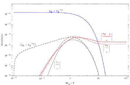
Figure 5: Comoving number density of triplets and antitriplets $\Sigma_{\Delta}$ and asymmetries $\Delta_{\Delta}$, $\Delta_{H}$ and $\Delta_{B-L}=\mbox{Tr}\,(\Delta_{\alpha\beta})$ as a function of $z=M_{\Delta}/T$, for $M_{\Delta}=5\times 10^{12}\,\mathrm{GeV}$, $\lambda_{H}=0.1$ and $m_{\Delta}=im_{\nu}$. Also shown is the departure of $\Sigma_{\Delta}$ from its equilibrium value. Asymmetries are plotted in units of the total CP asymmetry in triplet decays $\epsilon_{\Delta}$.

One can also express the baryon asymmetry of the universe in terms of the more familiar baryon-to-photon ratio $\eta_{B}\ \equiv n_{B}/n_{\gamma}=7.04\,\Delta_{B}$, whose observed value from recent Planck data is [58]

$$\eta^{\rm obs.}_{B}\,=\,(6.10\pm 0.06)\times 10^{-10}\qquad(68\%\,{\rm C.L.})\,.$$ (6.13)

As can be seen from Fig. 5, the $B-L$ asymmetry is already stabilized around $T\sim M_{\Delta}/100$.

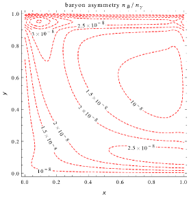
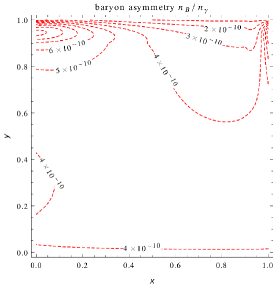
Figure 6: Isocurves of the baryon-to-photon ratio $n_{B}/n_{\gamma}$ in the $(x,y)$ plane for Ansatz 2. Left panel: $M_{\Delta}=5\times 10^{12}\,\mathrm{GeV}$, $\lambda_{H}=0.4$. Right panel: $M_{\Delta}=10^{11}\,\mathrm{GeV}$, $\lambda_{H}=0.025$.

We are now ready to present our numerical results. To reduce the number of free parameters, we concentrate on the ansätze defined in the previous subsection and fix the neutrino parameters as specifed there. Let us first consider Ansatz 2, which unlike Ansatz 1 does not maximize $\epsilon_{\Delta}$, but allows for larger flavour effects. Since this ansatz gives same-sign source terms in the Boltzmann equations, flavour effects are more likely to be relevant when $B_{\ell}\sim B_{H}$; hence, for a given triplet mass, we choose the parameter $\lambda_{H}$ such that $\lambda_{\ell}\sim\lambda_{H}$. Then we study the dependence of the baryon-to-photon ratio $n_{B}/n_{\gamma}$ on $x$ and $y$, the parameters that control the relative sizes of the couplings $f_{\alpha\beta}$. The result of the full computation (i.e. the computation involving the flavour-covariant Boltzmann equations with spectator processes included) is shown in Fig. 6 for two different values of the triplet mass, $M_{\Delta}=5\times 10^{12}\,\mathrm{GeV}$ and $M_{\Delta}=10^{11}\,\mathrm{GeV}$. For $M_{\Delta}=5\times 10^{12}\,\mathrm{GeV}$, $n_{B}/n_{\gamma}$ exceeds the observed value everywhere, but this can by cured by choosing a smaller overall phase in $m_{\Delta}$. We can see that the final baryon asymmetry is maximal for $x$ small and $y$ close to 1, more precisely around $(x,y)=(0.05,0.95)$, corresponding to $D_{\Delta}=\mbox{Diag}\,(0.949,0.0475,0.312)\,\bar{m}_{\nu}$. The baryon-to-photon ratio in this region is typically enhanced by a factor $2$ or $3$ with respect to Ansatz 1, although the total CP asymmetry is smaller. These conclusions are relatively stable under variations of the triplet mass as long as $B_{\ell}\sim B_{H}$.

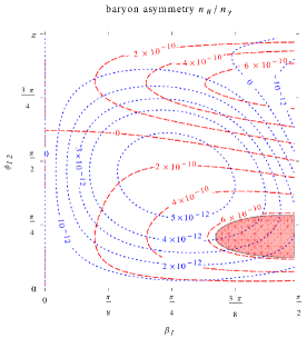
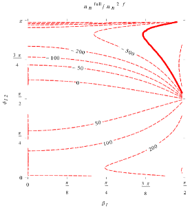
Figure 7: Left panel: the baryon-to-photon ratio $n_{B}/n_{\gamma}$ predicted by the full computation (red dashed lines) and by the 2-flavour approximation (blue dotted lines) as a function of $\beta_{1}$ and $\phi_{12}$ for Ansatz 3-a. The coloured areas indicate where the observed baryon asymmetry can be reproduced. Right panel: ratio of the full computation over the 2-flavour calculation of the baryon asymmetry. Along the solid curve, $n_{B}/n_{\gamma}$ vanishes in the 2-flavour approximation. In both panels, $M_{\Delta}=5\times 10^{11}\,\mathrm{GeV}$ and $\lambda_{H}=0.1$.

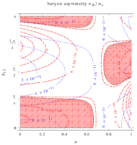
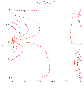
Figure 8: Left panel: the baryon-to-photon ratio $n_{B}/n_{\gamma}$ predicted by the full computation (red dashed lines) and by the 2-flavour approximation (blue dotted lines) as a function of $x$ and $\phi_{12}$ for Ansatz 3-b. The coloured areas indicate where the observed baryon asymmetry can be reproduced. Right panel: ratio of the full computation over the 2-flavour calculation of the baryon asymmetry. In both panels, $M_{\Delta}=5\times 10^{11}\,\mathrm{GeV}$ and $\lambda_{H}=0.1$.

We now proceed to study Ansatz 3, in which the CP asymmetry is concentrated in the $(\ell_{1},\ell_{2})$ subspace (i.e. $\mathcal{E}_{13}=\mathcal{E}_{23}=\mathcal{E}_{33}=0$ in the neutrino mass eigenstate basis). Let us first consider Ansatz 3-a, in which $D_{\Delta}=D_{\nu}$ while $\beta_{1}$ and $\phi_{12}$ can vary, all other phases and mixing angles in the unitary matrix $V$ being zero. We choose a triplet mass in the range [$10^{9}\,\mathrm{GeV},10^{12}\,\mathrm{GeV}$], and compare the result of the full computation with the one of the 2-flavour approximation, as described at the beginning of this section. As can be seen from Fig. 7, the baryon-to-photon ratio computed in a flavour-covariant way can be enhanced by up to a factor of several hundreds with respect to the 2-flavour approximation. Indeed, important flavour effects in the $e$–$\mu$ sector are missed in this approximation. This can be understood by examining a specific point of the parameter space, for instance $\phi_{12}=\pi/6$ and $\beta_{1}=\pi/2$. In the full computation, the sources terms in the Boltzmann equations (5.5) and (5.6) are proportional to

$$\mathcal{E}^{0}\,=\,\left(\begin{matrix}-10.36&-2.496\\ -2.496&6.846\end{matrix}\right)\times 10^{-8}\,,\qquad\mathcal{E}_{\tau\tau}\,=\,3.513\times 10^{-8}\,,$$ (6.14)

where for definiteness we have written $\mathcal{E}^{0}$ in the $(\ell_{e},\ell_{\mu})$ basis, while the flavour dependence of the washout is controlled by the triplet couplings to leptons:

$$\left(\begin{matrix}|f_{ee}|&|f_{e\mu}|&|f_{e\tau}|\\ |f_{\mu e}|&|f_{\mu\mu}|&|f_{\mu\tau}|\\ |f_{\tau e}|&|f_{\tau\mu}|&|f_{\tau\tau}|\end{matrix}\right)\,=\,\left(\begin{matrix}1.428&3.477&1.373\\ 3.477&9.288&9.394\\ 1.373&9.394&13.36\end{matrix}\right)\times 10^{-3}\,.$$ (6.15)

Thus we have a large source term for a flavour asymmetry (namely in the $e$ flavour) that is only weakly washed out by inverse decays. As a result, a large baryon asymmetry is generated ($n_{B}/n_{\gamma}=7.277\times 10^{-10}$) even though the total CP asymmetry vanishes (indeed, for the particular point considered $\epsilon_{\Delta}=\mbox{tr}\,\mathcal{E}^{0}+\mathcal{E}_{\tau\tau}=0$). By contrast, in the 2-flavour approximation, the CP asymmetries appearing in the Boltzmann equations (5.28) are

$$\epsilon_{0}\,=\,-3.513\times 10^{-8}\,=\,-\epsilon_{\tau}\,,$$ (6.16)

and the washout is controlled by

$$\left(\begin{matrix}f_{00}&f_{0\tau}\\ f_{0\tau}&|f_{\tau\tau}|\end{matrix}\right)\,=\,\left(\begin{matrix}10.69&9.567\\ 9.567&13.36\end{matrix}\right)\times 10^{-3}\,.$$ (6.17)

Therefore, the asymmetries stored in the two flavours are washed out with a comparable strength, and the resulting baryon asymmetry ($n_{B}/n_{\gamma}=1.617\times 10^{-12}$) is much smaller than in the full flavoured computation.

A similar (but numerically not as strong) enhancement of the full computation result with respect to the 2-flavour approximation can be observed for Ansatz 3-b, in which $D_{\Delta}=\text{Diag}(x\,m_{0},\sqrt{1-x^{2}}\,m_{0},m_{3})$ with $m_{0}=\sqrt{m^{2}_{1}+m^{2}_{2}}$ and the phases $\beta_{1}$ and $\beta_{2}$ are set to $\pi/4$. This is shown in Fig. 8.

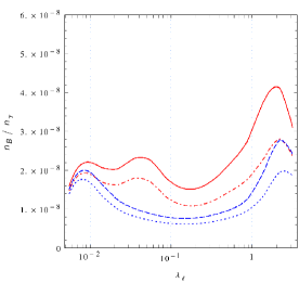
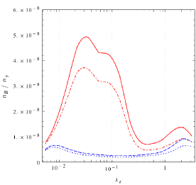
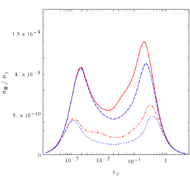
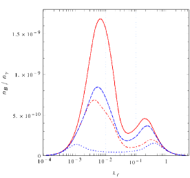
Figure 9: Baryon-to-photon ratio $n_{B}/n_{\gamma}$ as a function of $\lambda_{\ell}$ for $M_{\Delta}=5\times 10^{12}\,\mathrm{GeV}$, assuming Ansatz 1 (left panel) or Ansatz 2 with $(x,y)=(0.05,0.95)$ (right panel). The red lines indicate the result of the flavour-covariant computation involving the $3\times 3$ density matrix $\Delta_{\alpha\beta}$, with (solid red line) or without (dashed-dotted red line) spectator processes taken into account, whereas the blue lines indicate the result of the single flavour approximation, taking spectator processes into account (blue dashed line) or not (blue dotted line). The equality of branching ratios $B_{\ell}=B_{H}$ is realized for $\lambda_{\ell}\simeq 0.15$.

Figure 10: Baryon-to-photon ratio $n_{B}/n_{\gamma}$ as a function of $\lambda_{\ell}$ for $M_{\Delta}=10^{11}\,\mathrm{GeV}$, assuming Ansatz 1 (left panel) or Ansatz 2 with $(x,y)=(0.05,0.95)$ (right panel). The red lines indicate the result of the flavour-covariant computation involving the $2\times 2$ density matrix $\Delta^{0}_{\alpha\beta}$, with (solid red line) or without (dashed-dotted red line) spectator processes taken into account, whereas the blue lines indicate the result of the 2-flavour approximation, taking spectator processes into account (blue dashed line) or not (blue dotted line). The equality of branching ratios $B_{\ell}=B_{H}$ is realized for $\lambda_{\ell}\simeq 0.021$.

In Figs. 10 and 10, we compare the relative impacts of spectator processes and flavour covariance on the generated baryon asymmetry in the temperature regimes $T>10^{12}\,\mathrm{GeV}$ and $10^{9}\,\mathrm{GeV}<T<10^{12}\,\mathrm{GeV}$, respectively. We consider two ansätze designed to produce a large baryon asymmetry (even exceeding the observed value when the CP-violating phases are chosen to be large, as is the case here), namely Ansatz 1, which maximizes the total CP asymmetry, and Ansatz 2 with $(x,y)=(0.05,0.95)$, a parameter choice that has been shown to maximize the final baryon asymmetry in Fig. 6. In Fig. 10, the triplet mass has been chosen to be $M_{\Delta}=5\times 10^{12}\,\mathrm{GeV}$, so that most of the $B-L$ asymmetry is produced at $T>10^{12}\,\mathrm{GeV}$. For Ansatz 1 (i.e. $m_{\Delta}=im_{\nu}$), flavour effects and spectator processes have a quantitatively similar impact on the baryon-to-photon ratio, while for Ansatz 2 flavour effects strongly dominate over spectator processes such as QCD sphalerons or top quark Yukawa interactions (especially for $10^{-2}\lesssim\lambda_{\ell}\lesssim 0.5$). In this case, neglecting spectator processes and including flavour effects gives a much more accurate result than doing the opposite. In Fig. 10, the triplet mass is $M_{\Delta}=10^{11}\,\mathrm{GeV}$, hence the $B-L$ asymmetry is essentially generated in the temperature regime $10^{9}\,\mathrm{GeV}<T<10^{12}\,\mathrm{GeV}$ where the tau Yukawa coupling is in equilibrium, but the muon Yukawa coupling is not. For Ansatz 1, the 2-flavour calculation turns out to be a rather good approximation to the flavour-covariant computation, while neglecting spectator processes gives a very bad estimate, except for small or large values of $\lambda_{\ell}$. For Ansatz 2, on the contrary, both flavour covariance and spectator processes have a significant impact on the baryon-to-photon ratio (except again for extreme values of $\lambda_{\ell}$), and neglecting one of them underestimates the result by up to a factor 2. The 2-flavour approximation without spectator processes actually gives a much larger disagreement with the full computation.

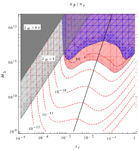
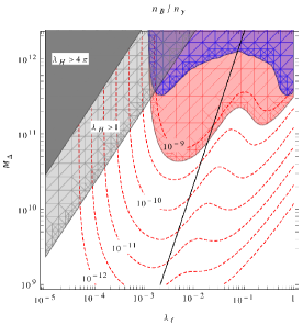
Figure 11: Isocurves of the baryon-to-photon ratio $n_{B}/n_{\gamma}$ in the $(\lambda_{\ell},M_{\Delta})$ plane obtained performing the full computation, assuming Ansatz 1 (left panel) or Ansatz 2 with $(x,y)=(0.05,0.95)$ (right panel). The coloured regions indicate where the observed baryon asymmetry can be reproduced in the full computation (light red shading) or in the single flavour approximation with spectator processes neglected (dark blue shading). The solid black line corresponds to $B_{\ell}=B_{H}$. Also shown are the regions where $\lambda_{H}$ is greater than $1$ or $4\pi$.

Finally, we study in Fig. 11 the dependence of the generated baryon asymmetry on $\lambda_{\ell}$ and $M_{\Delta}$, both for Ansatz 1 and for Ansatz 2 with $(x,y)=(0.05,0.95)$. The computation is performed assuming that the third generation Yukawa couplings as well as the charm Yukawa coupling are in equilibrium, which strictly speaking is true only in the temperature range $10^{9}\,\mathrm{GeV}<T<10^{12}\,\mathrm{GeV}$. From Fig. 11 one can conclude that successful scalar triplet leptogenesis is possible for a triplet mass as low as $4.4\times 10^{10}\,\mathrm{GeV}$, to be compared with $1.2\times 10^{11}\,\mathrm{GeV}$ in the approximation where flavour effects and spectator processes are neglected. Other assumptions about the flavour structure of the triplet couplings to leptons may allow for a lighter scalar triplet. For comparison, we quote the lower bounds found by Ref. [26] in the single flavour approximation with spectator processes neglected: $M_{\Delta}>1.3\times 10^{11}\,\mathrm{GeV}$ in the case $\bar{m}_{\Delta}=0.05\,\mathrm{eV}$ ($\approx\bar{m}_{\nu}$ for a hierarchical neutrino mass spectrum), in agreement with our result, and $M_{\Delta}>2.8\times 10^{10}\,\mathrm{GeV}$ in the case $\bar{m}_{\Delta}=0.001\,\mathrm{eV}\ll\bar{m}_{\nu}$. Although we did not consider ansätze satisfying $\bar{m}_{\Delta}\ll\bar{m}_{\nu}$, because flavour effects are comparatively smaller in this case, we also expect the latter bound to be lowered by the inclusion of flavour and spectator processes.

7 Conclusions

In this paper, we have shown how to consistently include the effects of the different lepton flavours in scalar triplet leptogenesis. When charged lepton Yukawa interactions are out of equilibrium at the time of leptogenesis, i.e. when the lepton asymmetry is generated at high temperature, the proper treatment of flavour effects involves a $3\times 3$ density matrix, whose evolution is governed by flavour-covariant Boltzmann equations. The often-used single flavour approximation, which gives rather accurate results in the standard leptogenesis scenario with right-handed neutrinos, leads to predictions for the generated baryon asymmetry that can depart by a large amount from the flavour-covariant computation. In the intermediate temperature regime where the tau Yukawa coupling is in equilibrium but the muon and the electron ones are not, the $3\times 3$ density matrix can be replaced by the asymmetry stored in the tau lepton doublet and by a $2\times 2$ density matrix describing the flavour asymmetries in the $(\ell_{e},\ell_{\mu})$ subspace and their quantum correlations. In this case too, the 2-flavour calculation in which the $(\ell_{e},\ell_{\mu})$ subspace is described by a single flavour $\ell_{0}$ does not in general give a good approximation of the flavour-covariant computation. Finally, when the tau and muon Yukawa couplings are in equilibrium, flavour covariance is completely broken and the dynamics of leptogenesis is described in terms of the asymmetries stored in the three lepton doublets $\ell_{e}$, $\ell_{\mu}$ and $\ell_{\tau}$.

We performed a numerical study of the impact of flavour effects and spectator processes on the generated baryon asymmetry for judiciously chosen ansätze, and compared the flavour-covariant computation with flavour non-covariant approximations used in the literature, with or without spectator processes included. We found discrepancies in the predictions for the baryon asymmetry ranging from an order one factor to two orders of magnitude. In particular, we showed that successful leptogenesis can easily be achieved when the decays of the triplet into leptons and Higgs bosons occur at a similar rate, while it would require a significantly heavier triplet in the single flavour approximation. As a result, the minimal triplet mass allowed by successful leptogenesis is lowered by the inclusion of flavour effects, from $1.2\times 10^{11}\,\mathrm{GeV}$ to $4.4\times 10^{10}\,\mathrm{GeV}$ in the case where the scalar triplet and the additional heavy states give comparable contributions to neutrino masses.

Throughout this paper, we worked in a framework in which the contribution of the additional heavy states to the CP asymmetries is parametrized by an effective dimension-5 operator, but the procedure we used to derive the flavour-covariant Boltzmann equations can also be applied to explicit models with e.g. several scalar triplets, or with a scalar triplet and right-handed neutrinos. The formalism employed in this paper can also be used to study the scenario of purely flavoured leptogenesis [30, 31] in a flavour-covariant way. In the framework used in this paper, this would require the addition of the effective four-lepton operator (2.15).

Acknowledgments

We thank Thomas Hambye for useful discussions. This work has been supported in part by the Agence Nationale de la Recherche under contract ANR 2010 BLANC 0413 01, by the European Research Council (ERC) Advanced Grant Higgs@LHC, and by the European Union FP7 ITN Invisibles (Marie Curie Actions, PITN-GA-2011-289442).

Appendix A Reaction densities

We summarize in this appendix some useful formulae for the reaction densities used in this paper. Let us first recall the general expression for the (thermally averaged) space-time density of a general reaction $a+b+\ldots\to i+j+\ldots\,$. Neglecting Bose enhancement and Pauli blocking factors:

$$\gamma(a+b+\ldots\rightarrow i+j+\ldots)\,=\int \frac{d^{3}p_{a}}{(2\pi)^{3}2\omega_{\vec{p}_{a}}}\rho^{\mathrm{eq}}_{a}\frac{d^{3}p_{b}}{2\omega_{\vec{p}_{b}}(2\pi)^{3}}\rho^{\mathrm{eq}}_{b}\dots\frac{d^{3}p_{i}}{2\omega_{\vec{p}_{i}}(2\pi)^{3}}\frac{d^{3}p_{j}}{2\omega_{\vec{p}_{j}}(2\pi)^{3}}\dots$$

$$|\mathcal{M}|^{2}\,(2\pi)^{4}\delta^{(4)}(p_{a}+p_{b}+\ldots-p_{i}-p_{j}-\ldots)\,,$$ (A.1)

where $|\mathcal{M}|^{2}$ is the squared matrix element summed over the internal degrees of freedom of the initial and final states, and $\rho^{\mathrm{eq}}_{X}(\vec{p})$ is the phase-space distribution function of the particle $X$ at kinetic and chemical equilibrium, which only depends on the bosonic or fermionic nature of $X$:

$$\rho^{\mathrm{eq}}_{\mathbin{\mathchoice{\ooalign{\raisebox{0.6pt}{\small{$\displaystyle B$}}\cr\smash{\raisebox{-0.6pt}{\small{$\displaystyle F$}}}\cr}}{\ooalign{\raisebox{0.6pt}{\small{$\textstyle B$}}\cr\smash{\raisebox{-0.6pt}{\small{$\textstyle F$}}}\cr}}{\ooalign{\raisebox{0.6pt}{\small{$\scriptstyle B$}}\cr\smash{\raisebox{-0.6pt}{\small{$\scriptstyle F$}}}\cr}}{\ooalign{\raisebox{0.6pt}{\small{$\scriptscriptstyle B$}}\cr\smash{\raisebox{-0.6pt}{\small{$\scriptscriptstyle F$}}}\cr}}}}(\vec{p})\,=\,\frac{1}{e^{\beta(E-\mu)}\mp 1}\,.$$ (A.10)

In the following all computations are done using the Maxwell-Boltzmann statistics, i.e. neglecting the difference between bosons and fermions:

$$\rho^{\mathrm{eq}}_{F}(\vec{p})\,=\,\rho^{\mathrm{eq}}_{B}(\vec{p})\,=\,e^{-\beta(E-\mu)}\,\equiv\,\rho^{\mathrm{eq}}_{\rm MB}(\vec{p})\,.$$ (A.11)

With this approximation, the space-time density of triplet and antitriplet decays can be written as

$$\gamma_{D}\,=\,s\Sigma_{\Delta}^{\mathrm{eq}}\,\frac{K_{1}(z)}{K_{2}(z)}\,\Gamma_{\Delta}\,,$$ (A.12)

where $\Sigma_{\Delta}\equiv(n_{\Delta}+n_{\bar{\Delta}})/s$ is the comoving number density of triplets and antitriplets, $K_{1,2}(z)$ are modified Bessel functions of the second kind, $z\equiv M_{\Delta}/T$ and $\Gamma_{\Delta}$ is the triplet decay width. For $2\to 2$ scatterings, one has

$$\gamma(a+b\rightarrow i+j)\,=\,\frac{T}{64\pi^{4}}\int_{s_{\mathrm{min}}}^{\infty}\!ds\,s^{1/2}\hat{\sigma}(s)\,K_{1}\!\left(\frac{\sqrt{s}}{T}\right),$$ (A.13)

where $\hat{\sigma}(s)=2s\,\lambda(1,m_{a}^{2}/s,m_{b}^{2}/s)\,\sigma(s)$ is the reduced cross-section summed over the internal degrees of freedom of initial and final particles.

When computing the space-time density of a $2\to 2$ scattering, one must take care to properly subtract the contribution of on-shell intermediate particles, which is already taken into account in decays and inverse decays [59]. When the resonance occurs in the $s$-channel, one can compute the subtracted reaction density by taking away the resonant part from the squared propagator in the narrow-width approximation [50, 5]:

$$|D|^{2}\ \rightarrow\ |D|^{2}-\frac{\pi}{M\Gamma}\delta\left(s-M^{2}\right),$$ (A.14)

where $M$ and $\Gamma$ are the mass and width of the intermediate particle, and $D$ is the propagator of the intermediate state in the Breit-Wigner form:

$$D\,=\,\frac{1}{s-M^{2}+iM\Gamma}\ .$$ (A.15)

We have to do this for the computation of $\gamma(\ell\ell\rightarrow\bar{H}\bar{H})$ and $\gamma(\ell\ell\rightarrow\ell\ell)$, which receive a contribution from $s$-channel triplet exchange. Similarly, when computing $\gamma(\ell\bar{\Delta}\rightarrow\ell\bar{\Delta})$, one has to subtract the contribution of real intermediate leptons in the $u$-channel, corresponding to the two processes $\bar{\Delta}\rightarrow\ell\ell$ and $\ell\ell\rightarrow\bar{\Delta}$. Following Ref. [5], we perform the subtraction in the following way:

$$|D|^{2}\ \rightarrow\ |D|^{2}-\frac{\pi}{E\Gamma_{\rm th}}\delta\left(u\right),$$ (A.16)

where $E$ is the energy of the intermediate lepton, $\Gamma_{\rm th}$ its thermal width, and the propagator of the intermediate lepton is

$$D\,=\,\frac{1}{u+iE\Gamma_{\rm th}}\ .$$ (A.17)

As in Ref. [5], we use the following representation of $\delta(x)$ in numerical computations:

$$\delta(x)\,=\,\frac{2}{\pi}\frac{\epsilon^{3}}{(x^{2}+\epsilon^{2})^{2}}\ ,$$ (A.18)

where $\epsilon$ is a small number. In the limit of small width, which we assume to be valid, one can simply set $\epsilon=\Gamma/M$ for a resonance in the $s$-channel with an intermediate particle of mass $M$ and width $\Gamma$, and $E\Gamma_{\rm th}=\epsilon M_{\Delta}^{2}$ for a resonance in the $u$-channel, with any small value for $\epsilon$. With this choice, one can compute the subtracted space-time densities for the various $2\to 2$ scatterings.

In what follows, we note $x\equiv s/M_{\Delta}^{2}$. The reduced cross-sections for the scatterings involving 2 leptons and 2 Higgs bosons are, after subtracting the contribution of the on-shell intermediate triplet,

$$(\hat{\sigma}^{\ell\ell}_{\bar{H}\bar{H}})^{\Delta}\, =\,\frac{3xM_{\Delta}^{2}}{8\pi v^{4}}\,\bar{m}_{\Delta}^{2}\,\frac{(1-x)^{2}-\epsilon^{2}}{[(1-x)^{2}+\epsilon^{2}]^{2}}\ ,$$

$$(\hat{\sigma}^{\ell\ell}_{\bar{H}\bar{H}})^{\mathcal{I}}\, =\,\frac{3xM_{\Delta}^{2}}{8\pi v^{4}}\,\mbox{Re}\!\left[\text{tr}(m_{\Delta}m_{\mathcal{H}}^{\dagger})\right]\frac{1-x}{(1-x)^{2}+\epsilon^{2}}\ ,$$ (A.19)

$$(\hat{\sigma}^{\ell\ell}_{\bar{H}\bar{H}})^{\mathcal{H}}\, =\,\frac{3xM_{\Delta}^{2}}{8\pi v^{4}}\,\bar{m}_{\mathcal{H}}^{2}\,,$$

for $\ell\ell\rightarrow\bar{H}\bar{H}$, and

$$(\hat{\sigma}^{\ell H}_{\bar{\ell}\bar{H}})^{\Delta}\, =\,\frac{3M_{\Delta}^{2}}{2\pi v^{4}}\,\bar{m}_{\Delta}^{2}\left(-\frac{1}{1+x}+\frac{\ln(1+x)}{x}\right),$$

$$(\hat{\sigma}^{\ell H}_{\bar{\ell}\bar{H}})^{\mathcal{I}}\, =\,\frac{3M_{\Delta}^{2}}{2\pi v^{4}}\,\mbox{Re}\!\left[\text{tr}(m_{\Delta}m_{\mathcal{H}}^{\dagger})\right]\!\left(1-\frac{\ln(1+x)}{x}\right),$$ (A.20)

$$(\hat{\sigma}^{\ell H}_{\bar{\ell}\bar{H}})^{\mathcal{H}}\, =\,\frac{3xM_{\Delta}^{2}}{4\pi v^{4}}\,\bar{m}_{\mathcal{H}}^{2}\,,$$

for $\ell H\rightarrow\bar{l}\bar{H}$, where the superscripts $\Delta$, $\mathcal{H}$ and $\mathcal{I}$ refer to the contributions of the scalar triplet, of the $D=5$ operator (2.13) responsible for $m_{\mathcal{H}}$ and to the interference between the two contributions, respectively. For the 2 lepton–2 lepton scatterings $\ell\ell\to\ell\ell$ and $\ell\bar{\ell}\to\ell\bar{\ell}$, we obtain

$$\hat{\sigma}^{\ell\ell}_{\ell\ell}\,=\,\frac{3}{32\pi}\,\lambda^{4}_{\ell}\,x^{2}\frac{(1-x)^{2}-\epsilon^{2}}{\left[(1-x)^{2}+\epsilon^{2}\right]^{2}}\ ,$$ (A.21)

and

$$\hat{\sigma}^{\ell\bar{\ell}}_{\ell\bar{\ell}}\,=\,\frac{3}{16\pi}\,\lambda^{4}_{\ell}\left(2+\frac{2}{1+x}-\frac{4}{x}\ln(1+x)\right).$$ (A.22)

We did not include the gauge contributions since they do not violate flavour, hence they drop from the Boltzmann equations. Finally, the reduced cross-sections for the scatterings $\ell\Delta\rightarrow\ell\Delta$, $\ell\bar{\Delta}\rightarrow\ell\bar{\Delta}$ and $\ell\bar{\ell}\rightarrow\Delta\bar{\Delta}$ are given by, after subtracting the contribution of the on-shell intermediate lepton in the $u$-channel,

$$\hat{\sigma}^{\ell\Delta}_{\ell\Delta}\, =\,\frac{9}{32\pi}\,\text{tr}[ff^{\dagger}ff^{\dagger}]\,\frac{(x-1)^{4}}{x^{4}}\ ,$$ (A.23)

$$\hat{\sigma}^{\ell\bar{\Delta}}_{\ell\bar{\Delta}}\, =\,\frac{9}{32\pi}\,\text{tr}[ff^{\dagger}ff^{\dagger}]\left[\,\ln\!\left(\frac{x^{2}\left((x-2)^{2}+\epsilon^{2}\right)}{x^{2}\epsilon^{2}+1}\right)+\frac{(x-1)^{2}}{x}\frac{4-2x}{(x-2)^{2}+\epsilon^{2}}\,\right],$$ (A.24)

$$\hat{\sigma}^{\Delta\bar{\Delta}}_{\ell\bar{\ell}}\, =\,\frac{9}{32\pi}\,\text{tr}[ff^{\dagger}ff^{\dagger}]\,\sqrt{1-\frac{4}{x}}\,\left[\,\frac{(x-2)}{\sqrt{(x-4)x}}\,\ln\!\left(\frac{x-2+\sqrt{x(x-4)}}{x-2-\sqrt{x(x-4)}}\right)-2\,\right].$$ (A.25)

With the above expressions, one can compute numerically the reaction densities $\gamma_{\ell H}$, $\gamma_{4\ell}$ and $\gamma_{\ell\Delta}$ that appear in the washout terms $\mathcal{W}^{\ell H}_{\alpha\beta}$, $\mathcal{W}^{4\ell}_{\alpha\beta}$ and $\mathcal{W}^{\ell\Delta}_{\alpha\beta}$, respectively (see Subsection 2.3 for the definition of these reaction densities and Eqs. (3.60), (3.61) and (3.62) for the washout terms). We also need the space-time density of triplet-antitriplet annihilations into Standard Model particles, $\gamma_{A}$, which enters the Boltzmann equation for $\Sigma_{\Delta}$, Eq. (3.68). The contribution of gauge scatterings to $\gamma_{A}$ has been computed in Ref. [26]. There are also subleading contributions proportional to $\lambda^{4}_{\ell}$, $\lambda^{4}_{H}$, $\lambda^{2}_{\ell}g^{2}_{a}$ and $\lambda^{2}_{H}g^{2}_{a}$, which we do not include in our computation.

Fig. 12 shows the typical magnitude of the various reaction densities and their evolution as a function of $z=M_{\Delta}/T$ (here for $M_{\Delta}=5\times 10^{12}\,\mathrm{GeV}$, $m_{\Delta}=im_{\nu}$ and $\lambda_{H}=0.2$). A ratio $\gamma_{R}/Hn_{\gamma}$ smaller than $1$ indicates that the reaction $R$ is slow on a cosmological time scale.

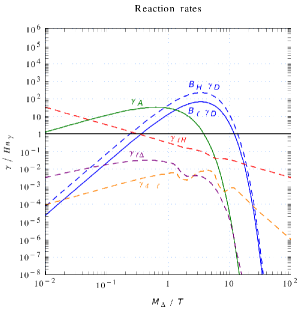
Figure 12: Space-time densities of decays ($B_{\ell}\gamma_{D}$, $B_{H}\gamma_{D}$) and scatterings ($\gamma_{A}$, $\gamma_{\ell H}$, $\gamma_{4\ell}$ and $\gamma_{\ell\Delta}$) in units of $Hn_{\gamma}$, as a function of $z=M_{\Delta}/T$, for the values of the parameters indicated in the text.

In this example, most scatterings are negligible, except for the ones involving Higgs bosons; however, the latter become slower than the expansion of the universe at the time where decays start to dominate over annihilations, a necesary condition for a large lepton asymmetry to develop [26, 32]. For the present choice of parameters, however, the third Sakharov condition would not be satisfied in the single flavour case, as both decays into Higgs bosons and into leptons are in equilibrium at the time of leptogenesis (i.e. at $z\lesssim 10$, before the triplet abundance becomes strongly Boltzmann-suppressed). Taking into account flavour effects leads to an enhanced efficiency because some “flavoured” decay channels $\Delta\to\bar{\ell}_{\alpha}\bar{\ell}_{\beta}$ are significantly slower than others.

References

- [1] M. Fukugita and T. Yanagida, Phys. Lett. B 174 (1986) 45.
- [2] S. Davidson, E. Nardi and Y. Nir, Phys. Rept. 466 (2008) 105 [arXiv:0802.2962 [hep-ph]].
- [3] W. Buchmuller and M. Plumacher, Phys. Lett. B 511 (2001) 74 [hep-ph/0104189].
- [4] E. Nardi, Y. Nir, J. Racker and E. Roulet, JHEP 0601 (2006) 068 [hep-ph/0512052].
- [5] G. F. Giudice, A. Notari, M. Raidal, A. Riotto and A. Strumia, Nucl. Phys. B 685 (2004) 89 [hep-ph/0310123].
- [6] R. Barbieri, P. Creminelli, A. Strumia and N. Tetradis, Nucl. Phys. B 575 (2000) 61 [hep-ph/9911315].
- [7] T. Endoh, T. Morozumi and Z. h. Xiong, Prog. Theor. Phys. 111 (2004) 123 [hep-ph/0308276].
- [8] A. Abada, S. Davidson, F. X. Josse-Michaux, M. Losada and A. Riotto, JCAP 0604 (2006) 004 [hep-ph/0601083].
- [9] E. Nardi, Y. Nir, E. Roulet and J. Racker, JHEP 0601 (2006) 164 [hep-ph/0601084].
- [10] A. Abada, S. Davidson, A. Ibarra, F.-X. Josse-Michaux, M. Losada and A. Riotto, JHEP 0609 (2006) 010 [hep-ph/0605281].
- [11] W. Buchmuller and S. Fredenhagen, Phys. Lett. B 483 (2000) 217 [hep-ph/0004145].
- [12] A. De Simone and A. Riotto, JCAP 0708 (2007) 002 [hep-ph/0703175].
- [13] M. Garny, A. Hohenegger, A. Kartavtsev and M. Lindner, Phys. Rev. D 80 (2009) 125027 [arXiv:0909.1559 [hep-ph]]; M. Garny, A. Hohenegger, A. Kartavtsev and M. Lindner, Phys. Rev. D 81 (2010) 085027 [arXiv:0911.4122 [hep-ph]].
- [14] V. Cirigliano, C. Lee, M. J. Ramsey-Musolf and S. Tulin, Phys. Rev. D 81 (2010) 103503 [arXiv:0912.3523 [hep-ph]].
- [15] M. Beneke, B. Garbrecht, M. Herranen and P. Schwaller, Nucl. Phys. B 838 (2010) 1 [arXiv:1002.1326 [hep-ph]].
- [16] M. Beneke, B. Garbrecht, C. Fidler, M. Herranen and P. Schwaller, Nucl. Phys. B 843 (2011) 177 [arXiv:1007.4783 [hep-ph]].
- [17] A. Anisimov, W. Buchmuller, M. Drewes and S. Mendizabal, Annals Phys. 326 (2011) 1998 [Erratum-ibid. 338 (2011) 376] [arXiv:1012.5821 [hep-ph]].
- [18] P. S. Bhupal Dev, P. Millington, A. Pilaftsis and D. Teresi, Nucl. Phys. B 891 (2015) 128 [arXiv:1410.6434 [hep-ph]].
- [19] T. Hambye, Y. Lin, A. Notari, M. Papucci and A. Strumia, Nucl. Phys. B 695 (2004) 169 [hep-ph/0312203].
- [20] W. Fischler and R. Flauger, JHEP 0809 (2008) 020 [arXiv:0805.3000 [hep-ph]].
- [21] A. Strumia, Nucl. Phys. B 809 (2009) 308 [arXiv:0806.1630 [hep-ph]].
- [22] D. Aristizabal Sierra, J. F. Kamenik and M. Nemevsek, JHEP 1010 (2010) 036 [arXiv:1007.1907 [hep-ph]].
- [23] D. V. Zhuridov, Int. J. Mod. Phys. A 28 (2013) 1350104 [arXiv:1204.4581 [hep-ph]].
- [24] T. Hambye and G. Senjanovic, Phys. Lett. B 582 (2004) 73 [hep-ph/0307237].
- [25] S. Antusch and S. F. King, Phys. Lett. B 597 (2004) 199 [hep-ph/0405093].
- [26] T. Hambye, M. Raidal and A. Strumia, Phys. Lett. B 632 (2006) 667 [hep-ph/0510008].
- [27] E. J. Chun and S. Scopel, Phys. Rev. D 75 (2007) 023508 [hep-ph/0609259].
- [28] T. Hallgren, T. Konstandin and T. Ohlsson, JCAP 0801 (2008) 014 [arXiv:0710.2408 [hep-ph]].
- [29] M. Frigerio, P. Hosteins, S. Lavignac and A. Romanino, Nucl. Phys. B 806 (2009) 84 [arXiv:0804.0801 [hep-ph]].
- [30] R. Gonzalez Felipe, F. R. Joaquim and H. Serodio, Int. J. Mod. Phys. A 28 (2013) 1350165 [arXiv:1301.0288 [hep-ph]].
- [31] D. Aristizabal Sierra, M. Dhen and T. Hambye, arXiv:1401.4347 [hep-ph].
- [32] T. Hambye, New J. Phys. 14 (2012) 125014 [arXiv:1212.2888 [hep-ph]].
- [33] A. D. Dolgov, Sov. J. Nucl. Phys. 33 (1981) 700 [Yad. Fiz. 33 (1981) 1309]; L. Stodolsky, Phys. Rev. D 36 (1987) 2273; G. Raffelt, G. Sigl and L. Stodolsky, Phys. Rev. Lett. 70 (1993) 2363 [Erratum-ibid. 98 (2007) 069902] [hep-ph/9209276]; G. Sigl and G. Raffelt, Nucl. Phys. B 406 (1993) 423.
- [34] M. Magg and C. Wetterich, Phys. Lett. B 94 (1980) 61; G. Lazarides, Q. Shafi and C. Wetterich, Nucl. Phys. B 181 (1981) 287; R. N. Mohapatra and G. Senjanovic, Phys. Rev. D 23 (1981) 165. See also J. Schechter and J. W. F. Valle, Phys. Rev. D 22 (1980) 2227.
- [35] A. D. Sakharov, Pisma Zh. Eksp. Teor. Fiz. 5 (1967) 32 [JETP Lett. 5 (1967) 24] [Sov. Phys. Usp. 34 (1991) 392] [Usp. Fiz. Nauk 161 (1991) 61].
- [36] P. J. O’Donnell and U. Sarkar, Phys. Rev. D 49 (1994) 2118 [hep-ph/9307279].
- [37] E. Ma and U. Sarkar, Phys. Rev. Lett. 80 (1998) 5716 [hep-ph/9802445].
- [38] S. Blanchet, P. Di Bari, D. A. Jones and L. Marzola, JCAP 1301 (2013) 041 [arXiv:1112.4528 [hep-ph]].
- [39] P. S. Bhupal Dev, P. Millington, A. Pilaftsis and D. Teresi, Nucl. Phys. B 886 (2014) 569 [arXiv:1404.1003 [hep-ph]].
- [40] E. K. Akhmedov, V. A. Rubakov and A. Y. Smirnov, Phys. Rev. Lett. 81 (1998) 1359 [hep-ph/9803255].
- [41] T. Asaka and M. Shaposhnikov, Phys. Lett. B 620 (2005) 17 [hep-ph/0505013].
- [42] A. De Simone and A. Riotto, JCAP 0702 (2007) 005 [hep-ph/0611357].
- [43] O. Vives, Phys. Rev. D 73 (2006) 073006 [hep-ph/0512160].
- [44] G. Engelhard, Y. Grossman, E. Nardi and Y. Nir, Phys. Rev. Lett. 99 (2007) 081802 [hep-ph/0612187].
- [45] A. Pilaftsis and T. E. J. Underwood, Phys. Rev. D 72 (2005) 113001 [hep-ph/0506107].
- [46] J. S. Schwinger, J. Math. Phys. 2 (1961) 407; L. V. Keldysh, Zh. Eksp. Teor. Fiz. 47 (1964) 1515 [Sov. Phys. JETP 20 (1965) 1018]; P. M. Bakshi and K. T. Mahanthappa, J. Math. Phys. 4 (1963) 1; P. M. Bakshi and K. T. Mahanthappa, J. Math. Phys. 4 (1963) 12.
- [47] V. Cirigliano, A. De Simone, G. Isidori, I. Masina and A. Riotto, JCAP 0801 (2008) 004 [arXiv:0711.0778 [hep-ph]].
- [48] K. c. Chou, Z. b. Su, B. l. Hao and L. Yu, Phys. Rept. 118 (1985) 1.
- [49] B. A. Campbell, S. Davidson, J. R. Ellis and K. A. Olive, Phys. Lett. B 297 (1992) 118 [hep-ph/9302221].
- [50] J. M. Cline, K. Kainulainen and K. A. Olive, Phys. Rev. D 49 (1994) 6394 [hep-ph/9401208].
- [51] G. D. Moore, Phys. Lett. B 412 (1997) 359 [hep-ph/9705248].
- [52] L. Bento, JCAP 0311 (2003) 002 [hep-ph/0304263].
- [53] S. Antusch, J. Kersten, M. Lindner, M. Ratz and M. A. Schmidt, JHEP 0503 (2005) 024 [hep-ph/0501272].
- [54] P. H. Chankowski and S. Pokorski, Int. J. Mod. Phys. A 17 (2002) 575 [hep-ph/0110249].
- [55] M. C. Gonzalez-Garcia, M. Maltoni and T. Schwetz, JHEP 1411 (2014) 052 [arXiv:1409.5439 [hep-ph]].
- [56] J. A. Harvey and M. S. Turner, Phys. Rev. D 42 (1990) 3344.
- [57] M. D’Onofrio, K. Rummukainen and A. Tranberg, Phys. Rev. Lett. 113 (2014) 14, 141602 [arXiv:1404.3565 [hep-ph]].
- [58] [Planck Collaboration], arXiv:1502.01589 [astro-ph.CO].
- [59] E. W. Kolb and S. Wolfram, Nucl. Phys. B 172 (1980) 224 [Erratum-ibid. B 195 (1982) 542].