Robust Group Linkage

Abstract

We study the problem of group linkage: linking records that refer to entities in the same group. Applications for group linkage include finding businesses in the same chain, finding conference attendees from the same affiliation, finding players from the same team, etc. Group linkage faces challenges not present for traditional record linkage. First, although different members in the same group can share some similar global values of an attribute, they represent different entities so can also have distinct local values for the same or different attributes, requiring a high tolerance for value diversity. Second, groups can be huge (with tens of thousands of records), requiring high scalability even after using good blocking strategies.

We present a two-stage algorithm: the first stage identifies cores containing records that are very likely to belong to the same group, while being robust to possible erroneous values; the second stage collects strong evidence from the cores and leverages it for merging more records into the same group, while being tolerant to differences in local values of an attribute. Experimental results show the high effectiveness and efficiency of our algorithm on various real-world data sets.

1 Introduction

Record linkage aims at linking records that refer to the same real-world entity and it has been extensively studied in the past years (surveyed in [8, 19]). In this paper we study a related but different problem that we call group linkage: linking records that refer to entities in the same group.

One major motivation for our work comes from identifying business chains–connected business entities that share a brand name and provide similar products and services (e.g., Walmart, McDonald’s). With the advent of the Web and mobile devices, we are observing a boom in local search; that is, searching local businesses under geographical constraints. Local search engines include Google Maps, Yahoo! Local, YellowPages, yelp, ezlocal, etc. The knowledge of business chains can have a big economic value to local search engines, as it allows users to search by business chain, allows search engines to render the returned results by chains, allows data collectors to clean and enrich information within the same chain, allows the associated review system to connect reviews on branches of the same chain, and allows sales people to target potential customers. Business listings are rarely associated with specific chains explicitly in real-world business-listing collections, so we need to identify the chains. Sharing the same name, phone number, or URL domain name can all serve as evidence of belonging to the same chain. However, for US businesses alone there are tens of thousands of chains and as we show soon, we cannot easily develop any rule set that applies to all chains.

We are also motivated by applications where we need to find people from the same organization, such as counting conference attendees from the same affiliation, counting papers by authors from the same institution, and finding players of the same team. The organization information is often missing, incomplete, or simply too heterogeneous to be recognized as the same (e.g., “International Business Machines Corporation”, “IBM Corp.”, “IBM”, “IBM Research Labs”, “IBM-Almaden”, etc., all refer to the same organization). Contact phones, email addresses, and mailing addresses of people all provide extra evidence for group linkage, but they can also vary for different people even in the same organization.

Group linkage faces challenges not present for traditional record linkage. First, although different members in the same group can share some similar global values of an attribute, they represent different entities so can also have distinct local values for the same or different attributes. For example, different branches in the same business chain can provide different local phone numbers, different addresses, etc. It is non-trivial to distinguish such differences from various representations for the same value and sometimes erroneous values in the data. Second, there are often millions of records for group linkage, and a group can contain tens of thousands of members. A good blocking strategy should put these tens of thousands of records in the same block; but performing record linkage via traditional pairwise comparisons within such huge blocks can be very expensive. Thus, scalability is a big challenge. We use the following example of identifying business chains throughout the paper for illustration.

Table 1: Identified top-5 US business chains. For each chain, we show the number of stores, distinct business names, distinct phone numbers, distinct URL domain names, and distinct categories.

Name	#Store	#Name	#Phn	#URL	#Cat
SUBWAY	21,912	772	21, 483	6	23
Bank of America	21,727	48	6,573	186	24
U-Haul	21,638	2,340	18,384	14	20
USPS - United State Post Office	19,225	12,345	5,761	282	22
McDonald’s	17,289	2401	16,607	568	47

Table 2: Real-world business listings. We show only state for location and simplify names of category. There is a wrong value in italic font.

RID	name	phone	URL (domain)	location	category
$r_{1}$	Home Depot, The	808		NJ	furniture
$r_{2}$	Home Depot, The	808		NY	furniture
$r_{3}$	Home Depot, The	808	homedepot	MD	furniture
$r_{4}$	Home Depot, The	808	homedepot	AK	furniture
$r_{5}$	Home Depot, The	808	homedepot	MI	furniture
$r_{6}$	Home Depot, The	101	homedepot	IN	furniture
$r_{7}$	Home Depot, The	102	homedepot	NY	furniture
$r_{8}$	Home Depot, USA	103	homedepot	WV	furniture
$r_{9}$	Home Depot USA	808		SD	furniture
$r_{10}$	Home Depot - Tools	808		FL	furniture
$r_{11}$	Taco Casa		tacocasa	AL	restaurant
$r_{12}$	Taco Casa	900	tacocasa	AL	restaurant
$r_{13}$	Taco Casa	900	tacocasa,	AL	restaurant
			tacocasatexas
$r_{14}$	Taco Casa	900		AL	restaurant
$r_{15}$	Taco Casa	900		AL	restaurant
$r_{16}$	Taco Casa	701	tacocasatexas	TX	restaurant
$r_{17}$	Taco Casa	702	tacocasatexas	TX	restaurant
$r_{18}$	Taco Casa	703	tacocasatexas	TX	restaurant
$r_{19}$	Taco Casa	704		NY	food store
$r_{20}$	Taco Casa		tacodelmar	AK	restaurant

Example 1.1

We consider a set of 18M real-world business listings in the US extracted from Yellowpages.com, each describing a business by its name, phone number, URL domain name, location, and category. Our algorithm automatically finds 600K business chains and 2.7M listings that belong to these chains. Table 1 lists the largest five chains we found. We observe that (1) each chain contains up to 22K different branch stores, (2) different branches from the same chain can have a large variety of names, phone numbers, and URL domain names, and (3) even chains of similar sizes can have very different numbers of distinct URLs (same for other attributes). Thus, rule-based linkage can hardly succeed and scalability is a necessity.

Table 2 shows a set of 20 business listings (with some abstraction) in this data set. After investigating their webpages manually, we find that $r_{1}-r_{18}$ belong to three business chains: $\mbox{Ch}_{1}=\{r_{1}-r_{10}\},\mbox{Ch}_{2}=\{r_{11}-r_{15}\}$, and $\mbox{Ch}_{3}=\{r_{16}-r_{18}\}$; $r_{19}$ and $r_{20}$ do not belong to any chain. Note the slightly different names for businesses in chain $\mbox{Ch}_{1}$; also note that $r_{13}$ is integrated from different sources and contains two URLs, one (tacocasatexas) being wrong.

Simple linkage rules do not work well on this data set. For example, if we require only high similarity on name for chain identification, we may wrongly decide that $r_{11}-r_{20}$ all belong to the same chain as they share a popular restaurant name Taco Casa. Traditional linkage strategies do not work well either. If we apply Swoosh-style linkage [27] and iteratively merge records with high similarity on name and shared phone or URL, we can wrongly merge $\mbox{Ch}_{2}$ and $\mbox{Ch}_{3}$ because of the wrong URL from $r_{13}$. If we require high similarity between listings on name, phone, URL, category, we may either split $r_{6}-r_{8}$ out of chain $\mbox{Ch}_{1}$ because of their different local phone numbers, or learn a low weight for phone but split $r_{9}-r_{10}$ out of chain $\mbox{Ch}_{1}$ since sharing the same phone number, the major evidence, is downweighted. $\Box$

The key idea in our solution is to find strong evidence that can glue group members together, while being tolerant to differences in values specific for individual group members. For example, we wish to reward sharing of primary values, such as primary phone numbers or URL domain names for chain identification, but would not penalize differences from local values, such as locations, local phone numbers, and even categories. For this purpose, our algorithm proceeds in two stages. First, we identify cores containing records that are very likely to belong to the same group. Second, we collect strong evidence from the resulting cores, such as primary phone numbers and URL domain names in business chains, based on which we cluster the cores and remaining records into groups. The use of cores and strong evidence distinguishes our clustering algorithm from traditional clustering techniques for record linkage. In this process, it is crucial that core generation makes very few false positives even in the presence of erroneous values, such that we can avoid ripple effect on clustering later. Our algorithm is designed to ensure efficiency and scalability.

The group linkage problem we study in this paper is different from the group linkage in [18, 23], which decides similarity between pre-specified groups of records. Our goal is to find records that belong to the same group and we make three contributions.

1. We study core generation in presence of erroneous data. Our core is robust in the sense that even if we remove a few possibly erroneous records from a core, we still have strong evidence that the rest of the records in the core must belong to the same group.

2. We then reduce the group linkage problem into clustering cores and remaining records. Our clustering algorithm leverages strong evidence collected from cores and meanwhile is tolerant to value variety of records in the same group.

3. We conducted experiments on two real-world data sets in different domains, showing high efficiency and effectiveness of our algorithms.

Note that we assume prior to group linkage, we first conduct record linkage (e.g., [15]). Our experiments show that minor mistakes for record linkage do not significantly affect the results of group linkage, and records that describe the same entity but fail to be merged in the record-linkage step are often put into the same group. We plan to study how to combine record linkage and group linkage to improve the results of both in the future.

In the rest of the paper, Section 2 discusses related work. Section 3 defines the problem and provides an overview of our solution. Sections 4-5 describe the two stages in our solution. Section 6 describes experimental results. Section 7 concludes.

2 Related Work

Record linkage has been extensively studied in the past (surveyed in [8, 19]). Traditional linkage techniques aim at linking records that refer to the same real-world entity, so implicitly assume value consistency between records that should be linked. Group linkage is different in that it aims at linking records that refer to different entities in the same group. The variety of individual entities requires better use of strong evidence and tolerance on different values even within the same group. These two features differentiate our work from any previous linkage technique.

For record clustering in linkage, existing work may apply the transitive rule [17], or do match-and-merge [27], or reduce it to an optimization problem [16]. Our work is different in that our core-identification algorithm aims at being robust to a few erroneous records; and our clustering algorithm emphasizes leveraging the strong evidence collected from the cores.

For record-similarity computation, existing work can be rule based
 [17], classification based [11], or distance based [6]. There has also been work on weight (or model) learning from labeled data [11, 29]. Our work is different in that in addition to learning a weight for each attribute, we also learn a weight for each value based on whether it serves as important evidence for the group. Note that some previous works are also tolerant to different values but leverage evidence that may not be available in our contexts: [10] is tolerant to schema heterogeneity from different relations by specifying matching rules; [15] is tolerant to possibly false values by considering agreement between different data providers; [21] is tolerant to out-of-date values by considering time stamps; we are tolerant to diversity within the same group.

Two-stage clustering has been proposed in the IR and machine learning community [1, 20, 22, 28, 30]; however, they identify cores in different ways. Techniques in [20, 28] consider a core as a single record, either randomly selected or selected according to the weighted degrees of nodes in the graph. Techniques in [30] generate cores using agglomerative clustering but can be too conservative and miss strong evidence. Techniques in [1] identify cores as bi-connected components, where removing any node would not disconnect the graph. Although this corresponds to the 1-robustness requirement in our solution (defined in Section 4), they generate overlapping clusters; it is not obvious how to derive non-overlapping clusters in applications such as business-chain identification and how to extend their techniques to guarantee $k$-robustness. Finally, techniques in [20, 22] require knowledge of the number of clusters for one of the stages, so do not directly apply in our context. We compare with these methods whenever applicable in experiments (Section 6), showing that our algorithm is robust in presence of erroneous values and consistently generates high-accuracy results on data sets with different features.

Finally, we distinguish our work from the group linkage in [18, 23], which has different goals. On et al. [23] decided similarity between pre-specified groups of records and the group-entity relationship is many-to-many (e.g., authors and papers). Huang [18] decided whether two pre-specified groups of records from different data sources refer to the same group by analysis of social network. Our goal is to find records that belong to the same group.

3 Overview

This section formally defines the group linkage problem and provides an overview of our solution.

3.1 Problem definition

Let $\bf R$ be a set of records that describe real-world entities by a set of attributes $\bf A$. For each record $r\in\bf R$, we denote by $r.A$ its value on attribute $A\in\bf A$. Sometimes a record may contain erroneous or missing values.

We consider the group linkage problem; that is, finding records that represent entities belonging to the same real-world group. As an example application, we wish to find business chains–a set of business entities with the same or highly similar names that provide similar products and services (e.g., Walmart, Home Depot, Subway and McDonald’s). We focus on non-overlapping groups, which often hold in applications.

Definition 3.1 (Group linkage)

Given a set $\bf R$ of records, group linkage identifies a set of clusters $\bf CH$ of records in $\bf R$, such that (1) records that represent real-world entities in the same group belong to one cluster, and (2) records from different groups belong to different clusters. $\Box$

Example 3.2

Consider records in Example 1.1, where each record describes a business store (at a distinct location) by attributes name, phone, URL, location, and category.

The ideal solution to the group linkage problem contains 5 clusters: $\mbox{Ch}_{1}=\{r_{1}-r_{10}\}$, $\mbox{Ch}_{2}=\{r_{11}-r_{15}\}$, $\mbox{Ch}_{3}=\{r_{16}-r_{18}\}$, $\mbox{Ch}_{4}=\{r_{19}\}$, and $\mbox{Ch}_{5}=\{r_{20}\}$. Among them, $\mbox{Ch}_{2}$ and $\mbox{Ch}_{3}$ represent two different chains with the same name. $\Box$

3.2 Overview of our solution

Group linkage is related to but different from traditional record linkage because it essentially looks for records that represent entities in the same group, rather than records that represent exactly the same entity. Different members in the same group often share a certain amount of commonality (e.g., common name, primary phone, and URL domain of chain stores), but meanwhile can also have a lot of differences (e.g., different addresses, local phone numbers, and local URL domains); thus, we need to allow much higher variety in some attribute values to avoid false negatives. On the other hand, as we have shown in Example 1.1, simply lowering our requirement on similarity of records or similarity of a few attributes in clustering can lead to a lot of false positives.

The key intuition of our solution is to distinguish between strong evidence and weak evidence. For example, different branches in the same business chain often share the same URL domain name and those in North America often share the same 1-800 phone number. Thus, a URL domain or phone number shared among many business listings with highly similar names can serve as strong evidence for chain identification. In contrast, a phone number shared by only a couple of business entities is much weaker evidence, since one might be an erroneous or out-of-date value.

To facilitate leveraging strong evidence, our solution consists of two stages. The first stage collects records that are highly likely to belong to the same group; for example, a set of business listings with the same name and phone number are very likely to be in the same chain. We call the results cores of the groups; from them we can collect strong evidence such as name, primary phone number, and primary URL domain of chains. The key goal of this stage is to be robust against erroneous values and make as few false positives as possible, so we can avoid identifying strong evidence wrongly and causing incorrect ripple effect later; however, we need to keep in mind that being too strict can miss important strong evidence.

The second stage clusters cores and remaining records into groups according to the discovered strong evidence. It decides whether several cores belong to the same group, and whether a record that does not belong to any core actually belongs to some group. It also employs weak evidence, but treats it differently from strong evidence. The key intuition of this stage is to leverage the strong evidence and meanwhile be tolerant to diversity of values in the same group, so we can reduce false negatives made in the first stage.

We next illustrate our approach for business-chain identification.

Example 3.3

Continue with the motivating example. In the first stage we generate three cores: $\mbox{Cr}_{1}=\{r_{1}-r_{7}\},\mbox{Cr}_{2}=\{r_{14},r_{15}\},\mbox{Cr}_{3}=\{r_{16}-r_{18}\}$. Records $r_{1}-r_{7}$ are in the same core because they have the same name, five of them ($r_{1}-r_{5}$) share the same phone number 808 and five of them ($r_{3}-r_{7}$) share the same URL homedepot. Similar for the other two cores. Note that $r_{13}$ does not belong to any core, because one of its URLs is the same as that of $r_{11}-r_{12}$, and one is the same as that of $r_{16}-r_{18}$, but except name, there is no other common information between these two groups of records. To avoid mistakes, we defer the decision on $r_{13}$. Indeed, recall that tacocasatexas is a wrong value for $r_{13}$. For a similar reason, we defer the decision on $r_{12}$.

In the second stage, we generate groups–business chains. We merge $r_{8}-r_{10}$ with core $\mbox{Cr}_{1}$, because they have similar names and share either the primary phone number or the primary URL. We also merge $r_{11}-r_{13}$ with core $\mbox{Cr}_{2}$, because (1) $r_{12}-r_{13}$ share the primary phone 900 with $\mbox{Cr}_{2}$, and (2) $r_{11}$ shares the primary URL tacocasa with $r_{12}-r_{13}$. We do not merge $\mbox{Cr}_{2}$ and $\mbox{Cr}_{3}$ though, because they share neither the primary phone nor the primary URL. We do not merge $r_{19}$ or $r_{20}$ to any core, because there is again not much strong evidence. We thus obtain the ideal result. $\Box$

To facilitate this two-stage solution, we find attributes that provide evidence for group identification and classify them into three categories.

• Common-value attribute: We call an attribute $A$ a common-value attribute if all entities in the same group have the same or highly similar $A$-values. Such attributes include business-name for chain identification and organization for organization linkage.

• Dominant-value attribute: We call an attribute $A$ a dominant-value attribute if entities in the same group often share one or a few primary $A$-values (but there can also exist other less-common values), and these values are seldom used by entities outside the group. Such attributes include phone and URL-domain for chain identification, and office-address, phone-prefix, and email-server for organization linkage.

• Multi-value attribute: We call the rest of the attributes mutli-value attributes as there is often a many-to-many relationship between groups and values of these attributes. Such attributes include category for chain identification.

The classification can be either learned from training data based on cardinality of attribute values, or performed by domain experts since there are typically only a few such attributes.

We describe core identification in Section 4 and group linkage in Section 5. Our algorithms require common-value and dominant-value attributes, which typically exist for groups in practice. While we present the algorithms for the setting of one machine, a lot of components of our algorithms can be easily parallelized in Hadoop infrastructure [24, 4]; it is not the focus of the paper and we briefly describe the opportunities in Section 6.4.

4 Core Identification

The first stage of our solution creates cores consisting of records that are very likely to belong to the same group. The key goal in core identification is to be robust to possible erroneous values. This section starts with presenting the criteria we wish the cores to meet (Section 4.1), then describes how we efficiently construct similarity graphs to facilitate core finding (Section 4.2), and finally gives the algorithm for core identification (Section 4.3). Note that the notations in this section can be slightly different from those in Graph Theory.

4.1 Criteria for a core

At the first stage we wish to make only decisions that are highly likely to be correct; thus, we require that each core contains only highly similar records, and different cores are fairly different and easily distinguishable from each other. In addition, we wish that our results are robust even in the presence of a few erroneous values in the data. In the motivating example, $r_{1}-r_{7}$ form a good core, because 808 and homedepot are very popular values among these records. In contrast, $r_{13}-r_{18}$ do not form a good core, because records $r_{14}-r_{15}$ and $r_{16}-r_{18}$ do not share any phone number or URL domain; the only “connector” between them is $r_{13}$, so they can be wrongly merged if $r_{13}$ contains erroneous values. Also, considering $r_{13}-r_{15}$ and $r_{16}-r_{18}$ as two different cores is risky, because (1) it is not very clear whether $r_{13}$ is in the same chain as $r_{14}-r_{15}$ or as $r_{16}-r_{18}$, and (2) these two cores share one URL domain name so are not fully distinguishable.

We capture this intuition with connectivity of a similarity graph. We define the similarity graph of a set $\bf R$ of records as an undirected graph, where each node represents a record in R, and an edge indicates high similarity between the connected records (we describe later what we mean by high similarity). Figure 1 shows the similarity graph for the motivating example.

Each core would correspond to a connected sub-graph of the similarity graph. We wish such a sub-graph to be robust such that even if we remove a few nodes the sub-graph is still connected; in other words, even if there are some erroneous records, without them we still have enough evidence showing that the rest of the records should belong to the same group. The formal definition goes as follows.

Definition 4.1 ($k$-robustness)

A graph $G$ is $k$-robust if after removing arbitrary $k$ nodes and edges to these nodes, $G$ is still connected. A clique or a single node is $k$-robust for any $k$. $\Box$

In Figure 1, the subgraph with nodes $r_{1}-r_{7}$ is 2-robust. That with $r_{11}-r_{18}$ is not 1-robust, as removing $r_{13}$ can disconnect it.

According to the definition, we can partition the similarity graph into a set of $k$-robust subgraphs. As we do not wish to split any core unnecessarily, we require the maximal $k$-robust partitioning:

Definition 4.2 (Maximal $k$-robust partitioning)

Let $G$ be a similarity graph. A partitioning of $G$ is a maximal $k$-robust partitioning if it satisfies the following properties.

1. Each node belongs to one and only one partition.

2. Each partition is $k$-robust.

3. The result of merging any partitions is not $k$-robust. $\Box$

Note that a data set can have more than one maximal $k$-robust partitioning. Consider $r_{11}-r_{18}$ in Figure 1. There are three maximal 1-robust partitionings: $\{\{r_{11}\},\{r_{12},r_{14}-r_{15}\},\{r_{13},r_{16}-r_{18}\}\}$; $\{\{r_{11}-r_{12}\},\{r_{14}-r_{15}\},\{r_{13},r_{16}-r_{18}\}\}$; and $\{\{r_{11}-r_{15}\},\{r_{16}-r_{18}\}\}$. If we treat each partitioning as a possible world, records that belong to the same partition in all possible worlds have high probability to belong to the same group and so form a core. Accordingly, we define a core as follows and can prove its $k$-robustness.

Definition 4.3 ($k$-Core)

Let $\bf R$ be a set of records and $G$ be the similarity graph of $\bf R$. The records that belong to the same subgraph in every maximal $k$-robust partitioning of $G$ form a $k$-core of $\bf R$. A core contains at least 2 records. $\Box$

Property 4.4

A $k$-core is $k$-robust. $\Box$

Proof 4.1.

If a $k$-core $C_{r}$ of $G$ is not $k$-robust, there exists a maximal $k$-robust partitioning in $G$, where two nodes $r$ and $r^{\prime}$ in $C_{r}$ are in different partitions of this partitioning (proved by Lemma 4.21). This conflicts with the fact that records in $C_{r}$ belong to the same partition in every maximal $k$-robust partitioning of $G$. Therefore, a $k$-core is $k$-robust.

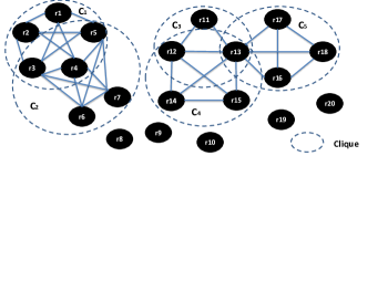
Figure 1: Similarity graph for records in Table 2.

Example 4.2.

Consider Figure 1 and assume $k=1$. There are two connected sub-graphs. For records $r_{1}-r_{7}$, the subgraph is 1-robust, so they form a $1$-core. For records $r_{11}-r_{18}$, there are three maximal 1-robust partitionings for the subgraph, as we have shown. Two subsets of records belong to the same subgraph in each partitioning: $\{r_{14}-r_{15}\}$ and $\{r_{16}-r_{18}\}$; they form 2 $1$-cores. $\Box$

Table 3: Simplified inverted index for the similarity graph in Figure 1.

Record	V-Cliques	Represent
$r_{1/2}$	$C_{1}$	$r_{1}-r_{2}$
$r_{3}$	$C_{1},C_{2}$	$r_{3}$
$r_{4}$	$C_{1},C_{2}$	$r_{4}$
$r_{5}$	$C_{1},C_{2}$	$r_{5}$
$r_{6/7}$	$C_{2}$	$r_{6}-r_{7}$
$r_{11}$	$C_{3}$	$r_{11}$
$r_{12}$	$C_{3},C_{4}$	$r_{12}$
$r_{13}$	$C_{3},C_{4},C_{5}$	$r_{13}$
$r_{14/15}$	$C_{4}$	$r_{14}-r_{15}$
$r_{16/17/18}$	$C_{5}$	$r_{16}-r_{18}$

4.2 Constructing similarity graphs

Generating the cores requires analysis on the similarity graph. Even after blocking, a block can contain tens of thousands of records, so it is not scalable to compare every pair of records in the same block and create edges accordingly. We next describe how we construct and represent the similarity graph in a scalable way.

We add an edge between two records if they have the same value for each common-value attribute and share at least one value on a dominant-value attribute; our experiments show advantages of this method over other edge-adding strategies (Section 6.2.1). All records that share values on the common-value attributes and share the same value on a dominant-value attribute form a clique, which we call a v-clique. We can thus represent the graph with a set of v-cliques, denoted by $\bf C$; for example, the graph in Figure 1 can be represented by 5 v-cliques ($C_{1}-C_{5}$). In addition, we maintain an inverted index $\bar{L}$, where each entry corresponds to a record $r$ and contains the v-cliques that $r$ belongs to. Whereas the size of the similarity graph can be quadratic in the number of the nodes, the size of the inverted index is only linear in that number. The inverted index also makes it easy to find adjacent v-cliques (i.e., v-cliques that share nodes), as they appear in the same entry.

Graph construction is then reduced to v-clique finding, which can be done by scanning values of dominant-value attributes. In this process, we wish to prune a v-clique if it is a sub-clique of another one. Pruning by checking every pair of v-cliques can be very expensive since the number of v-cliques is also huge. Instead, we do it together with v-clique finding. Specifically, our algorithm GraphConstruction takes $\bf R$ as input and outputs $\bf C$ and $\bar{L}$. We start with ${\bf C}=\bar{L}=\emptyset$. For each value $v$ of a dominant-value attribute, we denote the set of records with $v$ by $\bar{R}_{v}$ and do the following.

1. Initialize the v-cliques for $v$ as $\bf C_{v}=\emptyset$. Add a single-record cluster for each record $r\in\bar{R}_{v}$ to a working set $\bar{T}$. Mark each cluster as “unchanged”.

2. For each $r\in\bar{R}_{v}$, scan $\bar{L}$ and consider each v-clique $C\in\bar{L}(r)$ that has not been considered yet. For all records in $C\cap R_{v}$, merge their clusters. Mark the merged cluster as “changed” if the result is not a proper sub-clique of $\bar{C}$. If $C\subseteq\bar{R}_{v}$, remove $C$ from $\bf C$. This step removes the v-cliques that must be sub-cliques of those we will form next.

3. For each cluster $C\in\bar{T}$, if there exists $C^{\prime}\in\bf C_{v}$ such that $C$ and $C^{\prime}$ share the same value for each common-value attribute, remove $C$ and $C^{\prime}$ from $\bar{T}$ and $\bf C_{v}$ respectively, add $C\cup C^{\prime}$ to $\bar{T}$ and mark it as “changed”; otherwise, move $C$ to $\bf C_{v}$. This step merges clusters that share values on common-value attributes. At the end, $\bf C_{v}$ contains the v-cliques with value $v$.

4. Add each v-clique with mark “changed” in $\bf C_{v}$ to $\bf C$ and update $\bar{L}$ accordingly. The marking prunes size-1 v-cliques and the sub-cliques of those already in $\bf C$.

Proposition 4.3.

Let $\bf R$ be a set of records. Denote by $n(r)$ the number of values on dominant-value attributes from $r\in\bf R$. Let $n=\sum_{r\in\bf R}n(r)$ and $m=\max_{r\in\bf R}n(r)$. Let $s$ be the maximum v-clique size. Algorithm GraphConstruction (1) runs in time $O(ns(m+s))$, (2) requires space $O(n)$, and (3) its result is independent of the order in which we consider the records. $\Box$

Proof 4.4.

We first prove that GraphConstruction runs in time $O(ns(m+s))$. Step 2 of the algorithm takes in time $O(nsm)$, where it takes in time $O(ns)$ to scan all records for a dominant-value attribute, and a record can be scanned maximally $m$ times. Step 3 takes in time $O(ns^{2})$. Thus, the algorithm runs in time $O(ns(m+s))$.

We next prove that GraphConstruction requires space $O(n)$. For each value $v$ of a dominate-value attribute, the algorithm keeps three data sets: $\bar{L}$ that takes in space $O(n)$, $\bf C_{v}$ and $\bar{T}$ that require space in total no greater than $O(\bf|R|)$. Since $O(n)\geq O(\bf|R|)$, the algorithm requires space $O(n)$.

We now prove that the result of GraphConstruction is order independent. Given $\bar{L}$ and $\bar{R}_{v}$, Step 2 scan $\bar{L}$ and apply transitive rule to merge clusters of records in $C\cap\bar{R}_{v}$, for each v-clique $C\in\bar{L}$. The process is independent from the order in which we consider the records in $\bar{R}_{v}$. The order independence of the result in Step 3 is proven in [2]. Therefore, the final result is independent from the order in which we consider the records.

Example 4.5.

Consider graph construction for records in Table 2. Figure1 shows the similarity graph and Table 3(a) shows the inverted list. We focus on records $r_{1}-r_{8}$ for illustration.

First, $r_{1}-r_{5}$ share the same name and phone number 808, so we add v-clique $C_{1}=\{r_{1}-r_{5}\}$ to $\bf C$. Now consider URL homedepot where $\bar{R}_{v}=\{r_{3}-r_{8}\}$. Step 1 generates 6 clusters, each marked “unchanged”, and $\bar{T}=\{\{r_{3}\},\dots,\{r_{8}\}\}$. Step 2 looks up $\bar{L}$ for each record in $\bar{R}_{v}$. Among them, $r_{3}-r_{5}$ belong to v-clique $C_{1}$, so it merges their clusters and marks the result $\{r_{3}-r_{5}\}$ “unchanged” ($\{r_{3}-r_{5}\}\subset C_{1}$); then, $\bar{T}=\{\{r_{3}-r_{5}\},\{r_{6}\},\{r_{7}\},\{r_{8}\}\}$. Step 3 compares these clusters and merges the first three as they share the same name, marking the result as “changed”. At the end, ${\bf C}_{v}=\{\{r_{3}-r_{7}\},\{r_{8}\}\}$. Finally, Step 4 adds $\{r_{3}-r_{7}\}$ to $\bf C$ and discards $\{r_{8}\}$ since it is marked “unchanged”. $\Box$

Given the sheer number of records in $\bf R$, the inverted index can still be huge. In fact, according to the following theorem, records in the same v-clique but not any other v-clique must belong to the same core, so we do not need to distinguish them. Thus, we simplify the inverted index such that for each v-clique we keep only a representative for nodes belonging only to this v-clique. Table 3 shows the simplified index for the similarity graph in Figure 1.

Theorem 4.5.

Let $G$ be a similarity graph and $G^{\prime}$ be a graph derived from $G$ by merging nodes that belong to only one and the same $v$-clique. Two nodes belong to the same core of $G^{\prime}$ if and only if they belong to the same core of $G$. $\Box$

Proof 4.6.

We need to prove that (1) if two nodes $r$ and $r^{\prime}$ belong to the same core in $G^{\prime}$, they are in the same core of $G$, and (2) if two nodes $r$ and $r^{\prime}$ belong to the same core of $G$, they are in the same core of $G^{\prime}$.

We first prove that if two nodes $r$ and $r^{\prime}$ belong to the same core in $G^{\prime}$, they are in the same core of $G$. Suppose there does not exist any core in $G$ that contains both $r$ and $r^{\prime}$. It means that there exists a maximal $k$-robust partitioning in $G$, where $r$ and $r^{\prime}$ are in different partitions. Let $P$ be such a partitioning of $G$ and we consider partitioning $P^{\prime}$ of $G^{\prime}$, where each pair of nodes in the same partition $C$ of $P$ are in the same partition $C^{\prime}$ of $P^{\prime}$ and vice versa. We prove that $P^{\prime}$ is a maximal $k$-robust partitioning in $G^{\prime}$. (1) It is obvious that each node in $P^{\prime}$ belongs to one and only one partition. (2) For each partition $C^{\prime}$ in $P^{\prime}$, removing any $k$ nodes in $C^{\prime}$ is equivalent to removing $n+m$ nodes in $C$, where $n$ nodes belong to more than one $v$-cliques in $C$, $m$ nodes belong to single $v$-cliques in $C$, and $n\leq k$. Since removing $m$ nodes that belong to single $v$-cliques do not disconnect $C$ and we know $n\leq k$, removing the $n+m$ nodes does not disconnect $C$. It in turn proves that removing $k$ nodes in $C^{\prime}$ does not disconnect $C^{\prime}$, and $C^{\prime}$ is $k$-robust. (3) Similarly, we have that the result of of merging any partitions in $P^{\prime}$ is not $k$-robust. Therefore, $P^{\prime}$ is a maximal $k$-robust partitioning in $G^{\prime}$. Given that $r$ and $r^{\prime}$ are in different partitions of $P^{\prime}$, there does not exist a core of $G^{\prime}$ that contains both $r$ and $r^{\prime}$. This conflicts with the fact that $r$ and $r^{\prime}$ belong to the same core in $G^{\prime}$, and further proves that $r$ and $r^{\prime}$ are in the same core of $G$.

We next prove that if two nodes $r$ and $r^{\prime}$ belong to the same core of $G$, they are in the same core of $G^{\prime}$. Suppose there does not exist any core in $G^{\prime}$ that contains both $r$ and $r^{\prime}$. It means that there exists a maximal $k$-robust partitioning in $G^{\prime}$, where $r$ and $r^{\prime}$ are in different partitions. Let $P^{\prime}$ be such a partitioning of $G^{\prime}$ and we consider partitioning $P$ of $G$, where each pair of nodes in the same partition $C^{\prime}$ of $P^{\prime}$ are in the same partition $C$ of $P$ and vice versa. In similar ways as above, we have that $P$ is a maximal $k$-robust partitioning in $G$. Given that $r$ and $r^{\prime}$ are in different partitions of $P$, there does not exist a core of $G$ that contains both $r$ and $r^{\prime}$. This conflicts with the fact that $r$ and $r^{\prime}$ belong to the same core in $G$, and further proves that $r$ and $r^{\prime}$ are in the same core of $G^{\prime}$.

Case study: On a data set with 18M records (described in Section 6), our graph-construction algorithm finished in 1.9 hours. The original similarity graph contains 18M nodes and 4.2B edges. The inverted index is of size 89MB, containing 3.8M entries, each associated with at most 8 v-cliques; in total there are 1.2M v-cliques. The simplified inverted index is of size 34MB, containing 1.5M entries, where an entry can represent up to 11K records. Therefore, the simplified inverted index reduces the size of the similarity graph by 3 orders of magnitude.

4.3 Identifying cores

We solve the core-identification problem by reducing it to a Max-flow/Min-cut Problem. However, computing the max flow for a given graph $G$ and a source-destination pair takes time $O(|G|^{2.5})$, where $|G|$ denotes the number of nodes in $G$; even the simplified inverted index can still contain millions of entries, so it can be very expensive. We thus first merge certain v-cliques according to a sufficient (but not necessary) condition for $k$-robustness and consider them as a whole in core identification; we then split the graph into subgraphs according to a necessary (but not sufficient) condition for $k$-robustness. We apply reduction only on the resulting subgraphs, which are substantially smaller as we show at the end of this section. Section 4.3.1 describes screening before reduction, Section 4.3.2 describes the reduction, and Section 4.3.3 gives the full algorithm, which iteratively applies screening and the reduction.

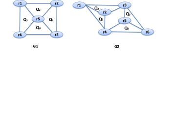
Figure 2: Two example graphs.

4.3.1 Screening

A graph can be considered as a union of v-cliques, so essentially we need to decide if a union of v-cliques is $k$-robust. First, we can prove the following sufficient condition for $k$-robustness.

Theorem 4.6 ($(K+1)$-connected condition).

Let $G$ be a graph consisting of a union $Q$ of v-cliques. If for every pair of v-cliques $C,C^{\prime}\in Q$, there is a path of v-cliques between $C$ and $C^{\prime}$ and every pair of adjacent v-cliques on the path share at least $k+1$ nodes, graph $G$ is $k$-robust. $\Box$

Proof 4.7.

Given Menger’s Theorem [3], graph $G$ is $k$-robust if for any pair of nodes $r,r^{\prime}$ in $G$, there exists at least $k+1$ independent paths that do not share any nodes other than $r,r^{\prime}$ in $G$. We now prove that for any pair of nodes $r,r^{\prime}$ in graph $G$ that satisfies $(k+1)$-connected condition, there exists at least $k+1$ independent paths between $r,r^{\prime}$. We consider two cases, 1) $r,r^{\prime}$ are adjacent such that there exists a v-clique in $G$ that contains $r,r^{\prime}$; 2) $r,r^{\prime}$ are not adjacent such that there exists no v-clique in $G$ that contains $r,r^{\prime}$.

We first consider Case 1 where there exists a v-clique $C$ containing $r,r^{\prime}$. Since each v-clique in $G$ has more than $k+1$ nodes, there exist at least $k$ 2-length paths and one 1-length path between $r,r^{\prime}\in C$. It proves that there exists at least $k+1$ independent paths between $r$ and $r^{\prime}$.

We next consider Case 2 where there exists no v-clique containing $r,r^{\prime}$ in $G$. Suppose $r\in C,r^{\prime}\in C^{\prime}$, where $C,C^{\prime}$ are different v-cliques in $G$. Since there exists a path of v-cliques between $C$ and $C^{\prime}$ where every pair of adjacent v-cliques in the path share at least $k+1$ nodes, there exists at least $k+1$ independent paths between $r$ and $r^{\prime}$.

Given the above two cases, we have that there exist at least $k+1$ independent paths between every pair of nodes in $G$, therefore $G$ is $k$-robust.

We call a single v-clique or a union of v-cliques that satisfy the $(k+1)$-connected condition a $(k+1)$-connected v-union. A $(k+1)$-connected v-union must be $k$-robust but not vice versa. In Figure 1, subgraph $\{r_{1}-r_{7}\}$ is a 3-connected v-union, because the only two v-cliques, $C_{1}$ and $C_{2}$, share 3 nodes. Indeed, it is 2-robust. On the other hand, graph $G_{1}$ in Figure 2 is 2-robust but not 3-connected (there are 4 v-cliques, where each pair of adjacent v-cliques share only 1 or 2 nodes). Accordingly, we can consider a v-union as a whole in core identification.

Next, we present a necessary condition for $k$-robustness.

Theorem 4.7 ($(K+1)$-overlap condition).

Graph $G$ is $k$-robust only if for every $(k+1)$-connected v-union $Q\in G$, $Q$ shares at least $k+1$ common nodes with the subgraph consisting of the rest of the v-unions. $\Box$

Proof 4.8.

We prove that if graph $G$ contains a $(k+1)$-connected v-union $Q$ that shares at most $k$ common nodes with the rest of the graph, $G$ is not $k$-robust. Since $Q$ shares at most $k$ common nodes with the subgraph consisting of the rest of the v-unions, removing the common nodes will disconnect $Q$ from $G$, it proves that $G$ is not $k$-robust. Thus, $(k+1)$-overlap condition holds.

We call a graph $G$ that satisfies the $(k+1)$-overlap condition a $(k+1)$-overlap graph. A $k$-robust graph must be a $(k+1)$-overlap graph but not vice versa. In Figure 1, subgraph $\{r_{11}-r_{18}\}$ is not a 2-overlap graph, because there are two 2-connected v-unions, $\{r_{11}-r_{15}\}$ and $\{r_{13},r_{16}-r_{18}\}$, but they share only one node; indeed, the subgraph is not 1-robust. On the other hand, graph $G_{2}$ in Figure 2 satisfies the 3-overlap condition, as it contains four 3-connected v-unions (actually four v-cliques), $Q_{1}-Q_{4}$, and each v-union shares 3 nodes in total with the others; however, it is not 2-robust (removing $r_{3}$ and $r_{4}$ disconnects it). Accordingly, for $(k+1)$-overlap graphs we still need to check $k$-robustness by reduction to a Max-flow Problem.

Now the problem is to find $(k+1)$-overlap subgraphs. Let $G$ be a graph where a $(k+1)$-connected v-union overlaps with the rest of the v-unions on no more than $k$ nodes. We split $G$ by removing these overlapping nodes. For subgraph $\{r_{11}-r_{18}\}$ in Figure 1, we remove $r_{13}$ and obtain two subgraphs $\{r_{11}-r_{12},r_{14}-r_{15}\}$ and $\{r_{16}-r_{18}\}$ (recall from Example 4.2 that $r_{13}$ cannot belong to any core). Note that the result subgraphs may not be $(k+1)$-overlap graphs (e.g., $\{r_{11}-r_{12},r_{14}-r_{15}\}$ contains two v-unions that share only one node), so we need to further screen them.

We now describe our screening algorithm, Screen (details in Algorithm 1), which takes a graph $G$, represented by $\bf C$ and $\bar{L}$, as input, finds $(k+1)$-connected v-unions in $G$ and meanwhile decides if $G$ is a $(k+1)$-overlap graph. If not, it splits $G$ into subgraphs for further examination.

1. If $G$ contains a single node, output it as a core if the node represents multiple records that belong only to one v-clique.

2. For each v-clique $C\in\bf C$, initialize a v-union. We denote the set of v-unions by $\bar{Q}$, the v-union that $C$ belongs to by $Q(C)$, and the overlapping nodes of $C$ and $C^{\prime}$ by $\bar{B}(C,C^{\prime})$.

3. For each v-clique $C\in\bf C$, we merge v-unions as follows.

   (a) For each record $r\in C$ that has not been considered, for every pair of v-cliques $C_{1}$ and $C_{2}$ in $r$’s index entry, if they belong to different v-unions, add $r$ to overlap $\bar{B}(C_{1},C_{2})$.

   (b) For each v-union $Q\neq Q(C)$ where there exist $C_{1}\in Q$ and $C_{2}\in Q(C)$ such that $|\bar{B}(C_{1},C_{2})|\geq k+1$, merge $Q$ and $Q(C)$.

   At the end, $\bar{Q}$ contains all $(k+1)$-connected v-unions.

4. For each v-union $Q\in\bar{Q}$, find its border nodes as $\bar{B}(Q)=\cup_{C\in Q,C^{\prime}\not\in Q}\bar{B}(C,C^{\prime})$. If $|\bar{B}(Q)|\leq k$, split the subgraph it belongs to, denoted by $G(Q)$, into two subgraphs $Q\setminus\bar{B}(Q)$ and $G(Q)\setminus Q$.

5. Return the remaining subgraphs.

Algorithm 1 Screening($G,\bar{C},\bar{L},k$)

0:  $G$: Simplified similarity graph. $\bar{C}$: Set of $k$-cores.$\bar{L}$: Inverted list of the similarity graph. $k$: Robustness requirement.

0:  $\bar{G}$ Set of subgraphs in $G$.

1:  if $G$ contains a single node $r$ then

2:     if $r$ represent multiple records then

3:        add $r$ to $\bar{C}$.

4:     end if

5:     return $\bar{G}=\phi$.

6:  else

7:     initialize v-union $Q(C)$ for each v-clique $C$ and add $Q(C)$ to $\bar{Q}$.

8:     // find v-union

9:     for each v-clique $C\in G$ do

10:        for each record $r\in C$ that is not proceeded do

11:           for each v-clique pair $C_{1},C_{2}\in\bar{L}(r)$ do

12:              if $C_{1},C_{2}$ are in different v-unions then

13:                 add $r$ to overlap $\bar{B}(Q(C_{1}),Q(C_{2}))$.

14:              end if

15:           end for

16:        end for

17:        for each v-union $Q$ where $\bar{B}(Q,Q(C))\geq k$ do

18:           merge $Q$ and $Q(C)$ as $Q_{m}$.

19:           for each v-union $Q^{\prime}\neq Q,Q^{\prime}\neq Q(C)$ do

20:              set $\bar{B}(Q^{\prime},Q_{m})=\bar{B}(Q^{\prime},Q)\cup\bar{B}(Q^{\prime},Q(C))$

21:           end for

22:        end for

23:     end for

24:     // screening

25:     for each v-union $Q\in\bar{Q}$ do

26:        compute $\bar{B}(Q)=\cup_{Q^{\prime}\in\bar{Q}}\bar{B}(Q,Q^{\prime})$.

27:        if $|\bar{B}(Q)|<k$ then

28:           add subgraphs $Q\setminus\bar{B}(Q)$ and $G(Q)\setminus Q$ into $\bar{G}$

29:        end if

30:     end for

31:  end if

32:  return  $\bar{G}$;

Proposition 4.9.

Denote by $|\bar{L}|$ the number of entries in input $\bar{L}$. Let $m$ be the maximum number of values from dominant-value attributes of a record, and $a$ be the maximum number of adjacent v-unions that a v-union has. Algorithm Screen finds $(k+1)$-overlap subgraphs in time $O((m^{2}+a)\cdot|\bar{L}|)$ and the result is independent of the order in which we examine the v-cliques. $\Box$

Proof 4.10.

We first prove the time complexity of Screen. It takes in time $O(m^{2}|\bar{L}|)$ to scan all entries in $\bar{L}$ and find common nodes between each pair of adjacent v-cliques (Step 3(a)). It takes in time $O(a|\bf C|)$ to merge v-unions, where $|\bf C|$ is the number of v-cliques in $G$ (Step 3(b)). Since $|\bf C|$ $<|\bar{L}|$, the algorithm runs in time $O(m^{2}+a)\cdot|\bar{L}|$.

We next prove that the result of $\sc Screen$ is independent of the order in which we examine the v-cliques, that is, 1) finding all maximal $(k+1)$-connected v-unions in $G$ is order independent; 2) removing all nodes in $\bar{B}(Q)$ from $G$ where $|\bar{B}(Q)|\leq k$ is order independent.

Consider order independency of finding all v-unions in $G$. To find all v-unions in $G$ is conceptually equivalent to find all connected components in an abstract graph $G_{A}$, where each node in $G_{A}$ is a v-clique in $G$ and two nodes in $G_{A}$ are connected if the two corresponding v-cliques share more than $k$ nodes. Screen checks whether each node in $G$ is a common node between two v-cliques (Step 3(a)), and if two cliques share more than $k$ nodes, merges their v-unions (Step 3(b)), which is equivalent to connect two nodes in $G_{A}$. Once all nodes in $G$ is scanned, all edges in $G_{A}$ are added, and the order in which we examine nodes in $G$ is independent from the structure of $G_{A}$ and the connected components in $G_{A}$. Therefore, finding all v-unions in $G$ is order independent.

Consider order independency of removing nodes in $G$. Suppose $Q_{1},Q_{2},...,Q_{m},m>0$ are all v-unions in $G$ with $|\bar{B}(Q_{i})|\leq k,i\in[1,m]$. Since $G$ is finite, $Q_{i}$ is finite and unique; thus, removing all nodes in $\bar{B}(Q))$ from $G$ where $|\bar{B}(Q)|\leq k$ is order independent.

Note that $m$ and $a$ are typically very small, so Screen is basically linear in the size of the inverted index. Finally, we have results similar to Theorem 4.5 for v-unions, so we can further simplify the graph by keeping for each v-union a single representative for all nodes that only belong to it. Each result $k$-overlap subgraph is typically very small.

Example 4.11.

Consider Table 3 as input and $k=1$. Step 2 creates five v-unions $Q_{1}-Q_{5}$ for the five v-cliques in the input.

Step 3 starts with v-clique $C_{1}$. It has 4 nodes (in the simplified inverted index), among which 3 are shared with $C_{2}$. Thus, $\bar{B}(C_{1},C_{2})=\{r_{3}-r_{5}\}$ and $|\bar{B}(C_{1},C_{2})|\geq 2$, so we merge $Q_{1}$ and $Q_{2}$ into $Q_{1/2}$. Examining $C_{2}$ reveals no other shared node.

Step 3 then considers v-clique $C_{3}$. It has three nodes, among which $r_{12}-r_{13}$ are shared with $C_{4}$ and $r_{13}$ is also shared with $C_{5}$. Thus, $\bar{B}(C_{3},C_{4})=\{r_{12}-r_{13}\}$ and $\bar{B}(C_{3},C_{5})=\{r_{13}\}$. We merge $Q_{3}$ and $Q_{4}$ into $Q_{3/4}$. Examining $C_{4}$ and $C_{5}$ reveals no other shared node. We thus obtain three 2-connected v-unions: $\bar{Q}=\{Q_{1/2},Q_{3/4},Q_{5}\}$.

Step 4 then considers each v-union. For $Q_{1/2}$, $\bar{B}(Q_{1/2})=\emptyset$ and we thus split subgraph $Q_{1/2}$ out and merge all of its nodes to one $r_{1/\dots/7}$. For $Q_{3/4}$, $\bar{B}(Q_{3/4})=\{r_{13}\}$ so $|\bar{B}(Q_{3/4})|<2$. We split $Q_{3/4}$ out and obtain $\{r_{11}-r_{12},r_{14/15}\}$ ($r_{13}$ is excluded). Similar for $Q_{5}$ and we obtain $\{r_{16/17/18}\}$. Therefore, we return three subgraphs for further screening. $\Box$

4.3.2 Reduction

Intuitively, a graph $G(V,E)$ is $k$-robust if and only if between any two nodes $a,b\in V$, there are more than $k$ paths that do not share any node except $a$ and $b$. We denote the number of non-overlapping paths between nodes $a$ and $b$ by $\kappa(a,b)$. We can reduce the problem of computing $\kappa(a,b)$ into a Max-flow Problem.

For each input $G(V,E)$ and nodes $a,b$, we construct the (directed) flow network $G^{\prime}(V^{\prime},E^{\prime})$ as follows.

1. Node $a$ is the source and $b$ is the sink (there is no particular order between $a$ and $b$).

2. For each $v\in V,v\neq a,v\neq b$, add two nodes $v^{\prime},v^{\prime\prime}$ to $V^{\prime}$, and two directed edges $(v^{\prime},v^{\prime\prime}),(v^{\prime\prime},v^{\prime})$ to $E^{\prime}$. If $v^{\prime}$ represents $n$ nodes, the edge $(v^{\prime},v^{\prime\prime})$ has weight $n$, and the edge $(v^{\prime\prime},v^{\prime})$ has weight $\infty$.

3. For each edge $(a,v)\in E$, add edge $(a,v^{\prime})$ to $E^{\prime}$; for each edge $(u,b)\in E$, add edge $(u^{\prime\prime},b)$ to $E^{\prime}$; for each other edge $(u,v)\in E$, add two edges $(u^{\prime\prime},v^{\prime})$ and $(v^{\prime\prime},u^{\prime})$ to $E^{\prime}$. Each edge has capacity $\infty$.

Lemma 4.12.

The max flow from source $a$ to sink $b$ in $G^{\prime}(V^{\prime},E^{\prime})$ is equivalent to $\kappa(a,b)$ in $G(V,E)$. $\Box$

Proof 4.13.

According to Menger’s Theorem [3], the minimum number of nodes whose removal disconnects $a$ and $b$, that is $\kappa(a,b)$, is equal to the maximum number of independent paths between $a$ and $b$. The authors in [9] proves that the maximum number of independent paths between $a$ and $b$ in an undirected graph $G(V,E)$ is equivalent to the maximal value of flow from $a$ to $b$ or the minimal capacity of an $a-b$ cut, the set of nodes such that any path from $a$ to $b$ contains a member of the cut, in $G^{\prime}(V^{\prime},E^{\prime})$.

Example 4.14.

Consider nodes $r_{1}$ and $r_{6}$ of graph $G_{2}$ in Figure 2. Figure 3 shows the corresponding flow network, where the dash line (across edges $(r_{3}^{\prime},r_{3}^{\prime\prime}),(r_{4}^{\prime},r_{4}^{\prime\prime})$) in the figure cuts the flow from $r_{1}$ to $r_{6}$ with a minimum cost of 2. The max flow/min cut has value 2. Indeed, $\kappa(r_{1},r_{6})=2$. $\Box$

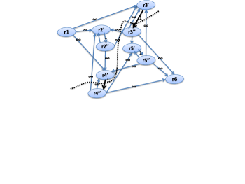
Figure 3: Flow network for $G_{2}$ in Figure 2.

Recall that in a $(k+1)$-connected v-union, between each pair of nodes there are at least $k+1$ paths. Thus, if (1) $\kappa(a,b)=k+1$, (2) $a$ and $b$ belong to different v-unions, and (3) $a$ and $a^{\prime}$ belong to the same v-union, we must have $\kappa(a^{\prime},b)\geq k+1$. We thus have the following sufficient and necessary condition for $k$-robustness.

Theorem 4.14 (Max-flow condition).

Let $G(V,E)$ be an input similarity graph. Graph $G$ is $k$-robust if and only if for every pair of adjacent $(k+1)$-connected v-unions $Q$ and $Q^{\prime}$, there exist two nodes $a\in Q\setminus Q^{\prime}$ and $b\in Q^{\prime}\setminus Q$ such that the max flow from $a$ to $b$ in the corresponding flow network is at least $k+1$. $\Box$

Proof 4.15.

According to Menger’s Theorem [3], $\kappa(a,b)$ in $G$ is equivalent to the max-flow from $a$ to $b$ in the corresponding flow network. We need to prove that graph $G$ is $k$-robust if and only if for each pair of adjacent $(k+1)$-connected v-unions $Q$ and $Q^{\prime}$, there exists two nodes $a\in Q\setminus Q^{\prime}$ and $b\in Q^{\prime}\setminus Q$ such that $\kappa(a,b)\geq k+1$.

We first prove that if $G$ is $k$-robust, for each pair of adjacent $(k+1)$-connected v-unions $Q$ and $Q^{\prime}$, there exists two nodes $a\in Q\setminus Q^{\prime}$ and $b\in Q^{\prime}\setminus Q$ such that $\kappa(a,b)\geq k+1$. Since $G$ is $k$-robust, for each pair of nodes $a$ and $b$ in $G$, we have $\kappa(a,b)\geq k+1$.

We next prove that if $G$ is not $k$-robust, there exists a pair of adjacent $(k+1)$-connected v-unions $Q$ and $Q^{\prime}$ such that for each pair of nodes $a\in Q\setminus Q^{\prime}$ and $b\in Q^{\prime}\setminus Q$, we have $\kappa(a,b)<k+1$. Since $G$ is not $k$-robust, there exists a separator $\bar{S}$, a set of nodes in $G$ with size no greater than $k$ whose removal disconnects $G$ into two sub-graphs $\bar{X}$ and $\bar{Y}$. Suppose $Q$ and $Q^{\prime}$ are two v-unions in $G$ such that $Q\subseteq\bar{X},Q^{\prime}\subseteq\bar{Y}$ and $Q\cap Q^{\prime}\neq\emptyset$. For each pair of nodes $a\in Q\setminus Q^{\prime}$ and $b\in Q^{\prime}\setminus Q$, we have $a\in\bar{X}$ and $b\in\bar{Y}$, and removing the set of nodes in $\bar{S}$ disconnects $a$ and $b$; thus $\kappa(a,b)<k+1$.

The above two cases proves that graph $G$ is $k$-robust if and only if for every pair of adjacent $(k+1)$-connected v-unions $Q$ and $Q^{\prime}$, there exist two nodes $a\in Q\setminus Q^{\prime}$ and $b\in Q^{\prime}\setminus Q$ such that $\kappa(a,b)\geq k+1$, i.e. the max flow from $a$ to $b$ in the corresponding flow network is at least $k+1$.

If a graph $G$ is not $k$-robust, we shall split it into subgraphs for further processing. In the corresponding flow network, each edge in the minimum cut must be between a pair of nodes derived from the same node in $G$ (other edges have capacity $\infty$). These nodes cannot belong to any core and we use them as separator nodes, denoted by $\bar{S}$. Suppose the separator separates $G$ into $\bar{X}$ and $\bar{Y}$ (there can be more subgraphs); we return $\bar{X}\cup\bar{S}$ and $\bar{Y}\cup\bar{S}$.

Note that we need to include $\bar{S}$ in both sub-graphs to maintain the integrity of each v-union. To understand why, consider $G_{2}$ in Figure 2 where $\bar{S}=\{r_{3},r_{4}\}$. According to the definition, there is no 2-core. If we split $G_{2}$ into $\{r_{1}-r_{2}\}$ and $\{r_{5}-r_{6}\}$ (without including $\bar{S}$), both subgraphs are 2-robust and we would return them as 2-cores. The problem happens because v-cliques $Q_{1}-Q_{4}$ “disappear” after we remove the separators $r_{3}$ and $r_{4}$. Thus, we should split $G_{2}$ into $\{r_{1}-r_{4}\}$ and $\{r_{3}-r_{6}\}$ instead and that would further trigger splitting on both subgraphs. Eventually we wish to exclude the separator nodes from any core, so we mark them as “separators” and exclude them from the returned cores.

Algorithm Split (details in Algorithm 2) takes a $(k+1)$-overlap subgraph $G$ as input and decides if $G$ is $k$-robust. If not, it splits $G$ into subgraphs on which we will then re-apply screening.

1. For each pair of adjacent $(k+1)$-connected v-unions $Q,Q^{\prime}\in G$, find $a\in Q\setminus Q^{\prime},b\in Q^{\prime}\setminus Q$. Construct flow network $G^{\prime}(V^{\prime},E^{\prime})$ and apply Ford & Fulkerson Algorithm [13] to compute the max flow.

2. Once we find nodes $a,b$ where $\kappa(a,b)\leq k$, use the min cut of the flow network as separator $\bar{S}$. Remove $\bar{S}$ and obtain several subgraphs. Add $\bar{S}$ back to each subgraph and mark $\bar{S}$ as “separator”. Return the subgraphs for screening.

3. Otherwise, $G$ is $k$-robust and output it as a $k$-core.

Algorithm 2 Split($G,\bar{C},k$)

0:  $G$: Simplified similarity graph. $\bar{C}$: Set of cores.$k$: Robustness requirement.

0:  $\bar{G}$ Set of subgraphs in $G$.

1:  for each adjacent $(k+1)$-connected v-unions $Q,Q^{\prime}$ do

2:     find a pair of nodes $a\in Q\setminus Q^{\prime},b\in Q^{\prime}\setminus Q$.

3:     construct flow-network $G^{\prime}$ and compute $\kappa(a,b)$ by Ford & Fulkerson Algorithm.

4:     if $\kappa(a,b)\leq k$ then

5:        get separator $\bar{S}$ from $G^{\prime}$ and remove $\bar{S}$ from $G$ to obtain disconnected subgraphs; mark $\bar{S}$ as “separator” and add it to each subgraph in $G$.

6:        return the set $\bar{G}$ of subgraphs.

7:     end if

8:  end for

9:  if $\bar{G}=\phi$ then

10:     add $G$ to $\bar{C}$.

11:  end if

12:  return  $\bar{G}$;

Example 4.16.

Continue with Example 4.14 and $k=2$. There are four 3-connected v-unions. When we check $r_{1}\in Q_{1}$ and $r_{6}\in Q_{3}$, we find $\bar{S}=\{r_{3},r_{4}\}$. We then split $G_{2}$ into subgraphs $\{r_{1}-r_{4}\}$ and $\{r_{3}-r_{6}\}$, marking $r_{3}$ and $r_{4}$ as “separators”.

Now consider graph $G_{1}$ in Figure 2 and $k=2$. There are four 3-connected v-unions (actually four v-cliques) and six pairs of adjacent v-unions. For $Q_{1}$ and $Q_{2}$, we check nodes $r_{2}$ and $r_{4}$ and find $\kappa(r_{2},r_{4})=3$. Similarly we check for every other pair of adjacent v-unions and decide that the graph is 2-robust. $\Box$

Proposition 4.17.

Let $p$ be the total number of pairs of adjacent v-unions, and $g$ be the number of nodes in the input graph. Algorithm Split runs in time $O(pg^{2.5})$. $\Box$

Proof 4.18.

Authors in [9] proves that it takes in time $O(g^{2.5})$ to compute $\kappa(a,b)$ for a pair of nodes $a$ and $b$ in $G$. In the worst case Split needs to compute $\kappa(a,b)$ for $p$ pairs of adjacent v-unions. Thus, Split runs in time $O(pg^{2.5})$.

Recall that if we solve the Max-Flow Problem directly for each pair of sources in the original graph, the complexity is $O(|\bar{L}|^{4.5})$, which would be dramatically higher.

4.3.3 Full algorithm

We are now ready to present the full algorithm, Core (Algorithm 3). Initially, it initializes the working queue $\bf Q$ with only input $G$ (Line 1). Each time it pops a subgraph $G^{\prime}$ from $\bf Q$ and invokes Screen (Lines 3-4). If the output of Screen is still $G^{\prime}$ (so $G^{\prime}$ is a $(k+1)$-overlap subgraph) (Line 5), it removes any node with mark “separator” in $G^{\prime}$ and puts the new subgraph into the working queue (Line 7), or invokes Split on $G^{\prime}$ if there is no separator (Line 9). Subgraphs output by Screen and Split are added to the queue for further examination (Lines 10, 13) and identified cores are added to $\bar{C}$, the core set. It terminates when $\bf Q=\emptyset$.

Algorithm 3 Core($G,k$)

0:  $G$: Simplified similarity graph, represented by $\bf C$ and $\bar{L}$. $k$: Robustness requirement.

0:  $\bar{C}$ Set of cores in $G$.

1:  Let ${\bf Q}=\{G\}$, $\bar{C}=\emptyset$;

2:  while $\bf Q\neq\phi$ do

3:     Pop $G^{\prime}$ from $\bf Q$;

4:     Let $\bar{P}=$ Screen($G^{\prime},k,\bar{C}$);

5:     if $\bar{P}=\{G^{\prime}\}$ then

6:        if $G^{\prime}$ contains “separator” nodes then

7:           Remove separators from $G^{\prime}$ and add the result to $\bf Q$ if it is not empty;

8:        else

9:           Let $\bar{S}=$ Split($G^{\prime},k,\bar{C}$);

10:           add graphs in $\bar{S}$ to $\bf Q$;

11:        end if

12:     else

13:        add graphs in $\bar{P}$ to $\bf Q$;

14:     end if

15:  end while

16:  return  $\bar{C}$;

The correctness of algorithm Core is guaranteed by the following Lemmas.

Lemma 4.19.

For each pair of adjacent nodes $r,r^{\prime}$ in graph $G$, there exists a maximal $k$-robust partitioning such that $r,r^{\prime}$ are in the same subgraph. $\Box$

Proof 4.20.

For each pair of adjacent nodes $r,r^{\prime}$ in $G$, we prove the existence of such a maximal $k$-robust partitioning by constructing it.

By definition, adjacent node $r,r^{\prime}$ form a v-clique $C$. Therefore, there exists a maximal v-clique $C^{\prime}$ in $G$ that contains $r,r^{\prime}$, i.e., $C\subseteq C^{\prime}$. V-clique $C^{\prime}$ can be obtained by keep adding nodes in $G$ to $C$ so that each newly-added node is adjacent to each node in current clique until no nodes in $G$ can be added to $C^{\prime}$. By definition, any v-clique is $k$-robust, therefore there exists a maximal $k$-robust sub-graph $G^{\prime}$ in $G$ such that $C^{\prime}\subseteq G^{\prime}$. Graph $G^{\prime}$ can be obtained by keep adding nodes in $G$ to $C^{\prime}$ so that each newly-added node is adjacent to at least $k+1$ nodes in current graph $G^{\prime}$ until no nodes in $G$ can be added to $G^{\prime}$. We remove $G^{\prime}$ from $G$ and take $G^{\prime}$ as a subgraph in the desired partitioning.

We repeat the above process to a randomly-selected pair of adjacent nodes in the remaining graph $G\setminus G^{\prime}$ until it is empty. The desired partitioning satisfies Condition 1 and 2 of Definition 4.2 because the above process makes sure each subgraph is exclusive and $k$-robust; it satisfies Condition 3 of Definition 4.2 because the above process makes sure each subgraph is maximal, which means merging arbitrary number of subgraphs in the partitioning would violate Condition 2.

In summary, the desired partitioning is a maximal $k$-robust partitioning. It proves that for each pair of adjacent nodes $r$ and $r^{\prime}$ in graph $G$, there exists a maximal $k$-robust partitioning such that $r$ and $r^{\prime}$ are in the same subgraph.

Lemma 4.21.

The set of nodes in a separator $\bar{S}$ of graph $G$ does not belong to any $k$-core in $G$, where $|\bar{S}|\leq k$. $\Box$

Proof 4.22 (Lemma 4.21).

Suppose the set $\bar{S}$ of nodes separate $G$ into $m$ disconnected sets $\bar{X}_{i},i\in[1,m],m>0$. To prove that each node $r\in\bar{S}$ does not belong to any $k$-core in $G$, we prove that for a node $r^{\prime}\in G,r^{\prime}\neq r$, there exists a maximal $k$-robust partitioning such that $r$ and $r^{\prime}$ are separated. Node $r^{\prime}$ falls into the following cases: 1) $r^{\prime}\in\bar{X}_{i},i\in[1,m]$ ; 2) $r^{\prime}\in\bar{S}$.

Consider Case 1) where $r^{\prime}\in\bar{X}_{i},i\in[1,m]$. We construct a maximal $k$-robust partitioning of $G$ where $r$ and $r^{\prime}$ are in different subgraphs. We start with a maximal $k$-robust subgraph $G^{\prime}$ in $G$ that contains $r$ and $r^{\prime\prime}$ where $r^{\prime\prime}$ is adjacent to $r$ and in $\bar{X}_{j},j\neq i,j\in[1,m]$, and find other maximal $k$-robust subgraphs as in Lemma 4.19. Since $\bar{S}$ separates $\bar{X}_{i}$ and $\bar{X}_{j}$, maximal $k$-robust subgraph $G^{\prime}$ that contains $r$ and $r^{\prime\prime}$ does not contain any node in $\bar{X}_{i}$. It proves that there exists a maximal $k$-robust partitioning of $G$ where $r$ and $r^{\prime}$ are not in the same subgraph.

Consider Case 2) where $r^{\prime}\in\bar{S}$. We construct a maximal $k$-robust partitioning of $G$ such that $r$ and $r^{\prime}$ are in different subgraphs. We create two maximal $k$-robust subgraphs $G^{\prime}$ and $G^{\prime\prime}$, where $G^{\prime}$ contains $r$ and an adjacent node $r_{i}\in\bar{X}_{i},i\in[1,m]$, $G^{\prime\prime}$ contains $r^{\prime}$ and an adjacent node $r_{j}\in\bar{X}_{j},j\neq i,j\in[1,m]$. We create other subgraphs as in Lemma 4.19. Since each path between $r_{i}\in\bar{X}_{i}$ and $r_{j}\in\bar{X}_{j}$ contains at least one node in $\bar{S}$ and $|\bar{S}|\leq k$, graph $G^{\prime}\cup G^{\prime\prime}$ is not $k$-robust. Therefore, the created partitioning is a maximal $k$-robust partitioning. It proves that there exists a maximal $k$-robust partitioning of $G$ where $r$ and $r^{\prime}$ are not in the same subgraph.

Given the above two cases, we have that any node in separator $\bar{S}$ of $G$ does not belong to any $k$-core in $G$, where $|\bar{S}|\leq k$.

Theorem 4.22.

Let $G$ be the input graph and $q$ be the number of $(k+1)$-connected v-unions in $G$. Define $a,p,g,m,$ and $|\bar{L}|$ as in Proposition 4.9 and 4.17. Algorithm Core finds correct $k$-cores of $G$ in time $O(q((m^{2}+a)|\bar{L}|+pg^{2.5}))$ and is order independent. $\Box$

Proof 4.23.

We first prove that Core correctly finds $k$-cores in $G$, that is 1) nodes not returned by Core do not belong to any $k$-core; 2) each subgraph returned by Core forms a $k$-core.

We prove that nodes not returned by Core do not belong to any $k$-core in $G$. Nodes not returned by Core belong to separators of subgraphs in $G$. Suppose $\bar{S}$ is a separator of graph $G_{n}\in\bf Q$ found in either Screen or Split phase, where $G_{n}\subseteq G,n\geq 0,G_{0}=G$, and $\bar{S}$ separates $G_{n}$ into $m$ sub-graphs $\bar{X}_{n}^{i},i\in[1,m],m>1$. Graph $G_{n}^{i}\in\bf Q$ is a subgraph of $G_{n}$ such that any node $r\in\bar{X}_{n}^{j},j\in[1,m],j\neq i$ does not belong to $G_{n}^{i}$. Nodes removed in $G_{n}^{i}$ by Core belong to separator $\bar{S}$ in $G_{n}$. Given Lema 4.21, such nodes do not belong to any $k$-core in $G_{n}$ and thus does not belong to any $k$-core in $G$.

We next prove that each subgraph returned by Core forms a $k$-core in $G$. We prove two cases: 1) subgraph $G^{\prime}$ in $G$ forms a $k$-core if there exists a separator $\bar{S}$ that disconnects $G^{\prime}$ from $G$, where $|\bar{S}|\leq k$ and $G^{\prime}\cup\bar{S}$ and $G^{\prime}$ are both $k$-robust; 2) if a subgraph is a $k$-core in $G_{n}^{i}$, it is a $k$-core in graph $G_{n}$.

We consider Case 1) that subgraph $G^{\prime}$ in $G$ forms a $k$-core if there exists a separator $\bar{S}$ that disconnects $G^{\prime}$ from $G$, where $|\bar{S}|\leq k$ and $G^{\prime}\cup\bar{S}$ and $G^{\prime}$ are both $k$-robust. For a pair of nodes $r_{1},r_{2}$ in $G^{\prime}$, we prove that there exists no maximal $k$-robust partitioning where $r_{1}$ and $r_{2}$ are in different subgraphs. Suppose such a partitioning exists, and $G_{1},G_{2}$ are subgraphs containing $r_{1},r_{2}$ respectively. Since $G_{1},G_{2}\subseteq G^{\prime}\cup\bar{S}$, we have that $G_{1}\cup G_{2}$ is $k$-robust, it violates the fact that the result of merging any two subgraphs in a maximal $k$-robust partitioning is not $k$-robust. Therefore, there exists no maximal $k$-robust partitioning where $r_{1}$ and $r_{2}$ are in different subgraphs. It proves that $G^{\prime}$ is a $k$-core in $G$.

We next consider Case 2) that if a subgraph $G^{\prime}$ is a $k$-core in $G_{n}^{i}$, it is a $k$-core in graph $G_{n}$. We prove that a pair of nodes $r_{1},r_{2}\in G^{\prime}$ belong to the same subgraph of all maximal $k$-robust partitioning in $G_{n}$. Suppose there exists such a partitioning of $G_{n}$ where $r_{1}\in G_{1},r_{2}\in G_{2}$. Since $G_{n}^{i}\subseteq\bar{X}_{n}^{i}\cup\bar{S}$, we have $G_{1},G_{2}\subseteq G_{n}^{i}$, otherwise $G_{1},G_{2}$ are not $k$-robust. Since $r_{1},r_{2}$ belong to the same $k$-core in $G_{n}^{i}$, we have $G_{1}=G_{2}$. It proves that if $G^{\prime}$ is a $k$-core in $G_{n}^{i}$, it is a $k$-core in $G_{n}$.

The above two cases prove that each subgraph returned by Core forms a $k$-core in $G$. In summary, nodes not returned by Core do not belong to any $k$-core, and each subgraph returned by Core forms a $k$-core in $G$. Thus, Core correctly finds all $k$-cores in $G$. It further proves that the result of Core is independent from the order in which we find and remove separators of graphs in $\bf Q$.

We now analyze the time complexity of Core. For each $(k+1)$-connected v-unions in $G$, it takes in time $O(m^{2}+a)|\bar{L}|$ to proceed Screen phase and in time $O(pg^{2.5})$ to proceed Split phase. In total there are $q$ v-unions in $G$, thus the algorithm takes in time $O(q((m^{2}+a)|\bar{L}|+pg^{2.5}))$.

Table 4: Step-by-step core identification in Example 4.24.

Input	Method	Output
$G_{2}$	Screen	$G_{2}$
$G_{2}$	Split	$G_{2}^{1}=\{r_{1}-r_{4}\},G_{2}^{2}=\{r_{3}-r_{6}\}$
$G_{2}^{1}$	Screen	$G_{2}^{3}=\{r_{3}\},G_{2}^{4}=\{r_{4}\}$
$G_{2}^{2}$	Screen	$G_{2}^{3}=\{r_{3}\},G_{2}^{4}=\{r_{4}\}$
$G_{2}^{3}$	Screen	-
$G_{2}^{4}$	Screen	-
$G$	Screen	$G^{1}=\{r_{1/\dots/7}\},G^{2}=\{r_{11},r_{12},r_{14/15}\},$
		$G^{3}=\{r_{16/17/18}\}$
$G^{1}$	Screen	Core $\{r_{1}-r_{7}\}$
$G^{2}$	Screen	$G^{4}=\{r_{11}\},G^{5}=\{r_{14/15}\}$
$G^{3}$	Screen	Core $\{r_{16}-r_{18}\}$
$G^{4}$	Screen	-
$G^{5}$	Screen	Core $\{r_{14}-r_{15}\}$

Example 4.24.

First, consider graph $G_{2}$ in Figure 2 and $k=2$. Table 4 shows the step-by-step core identification process. It passes screening and is the input for split. Split then splits it into $G_{2}^{1}$ and $G_{2}^{2}$, where $r_{3}$ and $r_{4}$ are marked as “separators”. Screen further splits each of them into $\{r_{3}\}$ and $\{r_{4}\}$, both discarded as each represents a single node (and is a separator). So Core does not output any core.

Next, consider the motivating example, with the input shown in Table 3 and $k=1$. Originally, ${\bf Q}=\{G\}$. After invoking Screen on $G$, we obtain three subgraphs $G^{1},G^{2},$ and $G^{3}$. Screen outputs $G^{1}$ and $G^{3}$ as 1-cores since each contains a single node that represents multiple records. It further splits $G^{2}$ into two single-node graphs $G^{4}$ and $G^{5}$, and outputs the latter as a 1-core. Note that if we remove the 1-robustness requirement, we would merge $r_{11}-r_{18}$ to the same core and get false positives. $\Box$

Case study: On the data set with 18M records, our core-identification algorithm finished in 2.2 minutes. Screen was invoked 114K times and took 2 minutes (91%) in total. Except the original graph, an input contains at most 39.3K nodes; for 97% inputs there are fewer than 10 nodes and running Screen was very fast. Split was invoked only 26 times; an input contains at most 65 nodes (13 v-unions) and on average 7.8 (2.7 v-unions). Recall that the simplified inverted index contains 1.5M entries, so Screen reduced the size of the input to Split by 4 orders of magnitude.

5 Group Linkage

The second stage clusters the cores and the remaining records, which we call satellites, into groups. To avoid merging records based only on weak evidence, we require that a cluster cannot contain more than one satellite but no core. Comparing with clustering in traditional record linkage, our algorithm differs in three aspects. First, in addition to weighting each attribute, we weight the values according to their popularity within a group such that similarity on primary values (strong evidence) is rewarded more. Second, we treat all values for dominant-value attributes as a whole, we are tolerant to differences on local values from different entities in the same group. Third, we distinguish weights for distinct values and non-distinct values such that similarity on distinct values is rewarded more. This section first describes the objective function for clustering (Section 5.1) and then proposes a greedy algorithm for clustering (Section 5.2).

5.1 Objective function

SV-index: Ideally, we wish that each cluster is cohesive (each element, being a core or a satellite, is close to other elements in the same cluster) and different clusters are distinct (each element is fairly different from those in other clusters). Since records in the same group may have fairly different local values, we adopt Silhouette Validation Index (SV-index) [25] as the objective function as it is more tolerant to diversity within a cluster. Given a clustering $\cal C$ of elements $\bf E$, the SV-index of $\cal C$ is defined as follows.

$$S(\cal C) = Avg_{e\in{\bf E}}S(e);$$ (1)

$$S(e) = \frac{a(e)-b(e)+\alpha}{\max\{a(e),b(e)\}+\beta}.$$ (2)

Here, $a(e)\in[0,1]$ denotes the similarity between element $e$ and its own cluster, $b(e)\in[0,1]$ denotes the maximum similarity between $e$ and another cluster, $\beta>\alpha>0$ are small numbers to keep $S(e)$ finite and non-zero (we discuss in Section 6 how we set the parameters). A nice property of $S(e)$ is that it falls in $[-1,1]$, where a value close to $1$ indicates that $e$ is in an appropriate cluster, a value close to $-1$ indicates that $e$ is mis-classified, and a value close to $0$ while $a(e)$ is not too small indicates that $e$ is equally similar to two clusters that should possibly be merged. Accordingly, we wish to obtain a clustering with the maximum SV-index. We next describe how we compare an element with a cluster.

Similarity computation: We consider that an element $e$ is similar to a cluster $Cl$ if they have highly similar values on common-value attributes (e.g., name), share at least one primary value (we explain “primary” later) on dominant-value attributes (e.g., phone, URL); in addition, our confidence is higher if they also share values on multi-value attributes (e.g., category). Following previous work on handling multi-value attributes [7, 21], we compute the similarity $sim(e,Cl)$ as follows.

$$sim(e,Cl) = \min\{1,sim_{s}(e,Cl)+\tau w_{m}sim_{multi}(e,Cl)\};$$ (3)

$$sim_{s}(e,Cl) = \frac{w_{c}sim_{com}(e,Cl)+w_{o}sim_{dom}(e,Cl)}{w_{c}+w_{o}};$$ (4)

$$\tau = \left\{\begin{array}[]{rl}0&\text{if}\ sim_{s}(e,Cl)<\theta_{th},\\ 1&\text{otherwise}.\end{array}\right.$$ (7)

Here, $sim_{com},sim_{dom},$ and $sim_{multi}$ denote the similarity for common-, dominant-, and multi-attributes respectively. We take the weighted sum of $sim_{com}$ and $sim_{dom}$ as strong indicator of $e$ belonging to $Cl$ (measured by $sim_{s}(e,Cl)$), and only reward weak indicator $sim_{multi}$ if $sim_{s}(e,Cl)$ is above a pre-defined threshold $\theta_{th}$; the similarity is at most 1. Weights $0<w_{c},w_{o},w_{m}<1$ indicate how much we reward value similarity or penalize value difference; we learn the weights from sampled data. We next highlight how we leverage strong evidence from cores and meanwhile remain tolerant to other different values in similarity computation.

First, we identify primary values (strong evidence) as popular values within a cluster. When we maintain the signature for a core or a cluster, we keep all values of an attribute and assign a high weight to a popular value. Specifically, let $\bar{R}$ be a set of records. Consider value $v$ and let $\bar{R}(v)\subseteq\bar{R}$ denote the records in $\bar{R}$ that contain $v$. The weight of $v$ is computed by $w(v)={|\bar{R}(v)|\over|\bar{R}|}$.

Example 5.1.

Consider phone for core $\mbox{Cr}_{1}=\{r_{1}-r_{7}\}$ in Table 2. There are $7$ business listings in $\mbox{Cr}_{1}$, $5$ providing 808 ($r_{1}-r_{5}$), one providing 101 ($r_{6}$), and one providing 102 ($r_{7}$). Thus, the weight of 808 is $\frac{5}{7}=.71$ and the weight for 101 and 102 is ${1\over 7}=.14$, showing that 808 is the primary phone for $\mbox{Cr}_{1}$. $\Box$

Second, when we compute $sim_{dom}(e,Cl)$, we consider all the dominant-value attributes together, rewarding sharing primary values (values with a high weight) but not penalizing different values unless there is no shared value. Specifically, if the primary value of an element is the same as that of a cluster, we consider them having probability $p$ to be in the same group. Since we use weights to measure whether the value is primary and allow slight difference on values, with a value $v$ from $e$ and $v^{\prime}$ from $Cl$, the probability becomes $p\cdot w_{e}(v)\cdot w_{Cl}(v^{\prime})\cdot s(v,v^{\prime})$, where $w_{e}(v)$ measures the weight of $v$ in $e$, $w_{Cl}(v^{\prime})$ measures the weight of $v^{\prime}$ in $Cl$, and $s(v,v^{\prime})$ measures the similarity between $v$ and $v^{\prime}$. We compute $sim_{dom}(r,Cl)$ as the probability that they belong to the same group given several shared values as follows.

$$sim_{dom}(e,Cl)=1-\prod_{v\in e,v^{\prime}\in ch}(1-p\cdot w_{e}(v)\cdot w_{Cl}(v^{\prime})\cdot s(v,v^{\prime})).$$ (8)

When there is no shared primary value, $sim_{dom}$ can be close to 0; once there is one such value, $sim_{dom}$ can be significantly increased, since we typically set a large $p$.

Example 5.2.

Consider element $e=r_{8}$ and cluster $\mbox{Cl}_{1}=\{r_{1}-r_{7}\}$ in Example 1.1. Assume $p=.9$. Element $e$ and $\mbox{Cl}_{1}$ share the primary email domain, with weight $1$ and ${5\over 7}=.71$ respectively, but have different phone numbers (assuming similarity of 0). We compute $sim_{dom}(e,\mbox{Cl}_{1})=1-(1-.9\cdot 1\cdot.71\cdot 1)\cdot(1-0)\cdot(1-0)\cdot(1-0)=.639$; essentially, we do not penalize the difference in phone numbers. Note however if homedepot appeared only once so was not a primary value, its weight would be $.14$ and accordingly $sim_{dom}(e,\mbox{Cl}_{1})=.126$, indicating a much lower similarity. $\Box$

Third, when we learn weights, we learn one set of weights for distinct values (appearing in only one cluster) and one set for non-distinct values, such that distinct values, which can be considered as stronger evidence, typically contribute more to the final similarity. In Example 1.1, sharing “Home Depot, The” would serve as stronger evidence than sharing Taco Casa for group similarity.

5.2 Clustering algorithm

In most cases, clustering is intractable [14, 26]. We maximize the SV-index in a greedy fashion. Our algorithm starts with an initial clustering and then iteratively examines if we can improve the current clustering (increase SV-index) by merging clusters or moving elements between clusters. According to the definition of SV-index, in both initialization and adjusting, we always assign an element to the cluster with which it has the highest similarity.

Initialization: Initially, we (1) assign each core to its own cluster and (2) assign a satellite $r$ to the cluster with the highest similarity if the similarity is above threshold $\theta_{ini}$ and create a new cluster for $r$ otherwise. We update the signature of each core along the way. Note that initialization is sensitive in the order we consider the records. Although designing an algorithm independent of the ordering is possible, such an algorithm is more expensive and our experiments show that the iterative adjusting can smooth out the difference.

Example 5.3.

Continue with the motivating example in Table 2. First, consider records $r_{1}-r_{10}$, where $\mbox{Cr}_{1}=\{r_{1}-r_{7}\}$ is a core. We first create a cluster $\mbox{Cl}_{1}$ for $\mbox{Cr}_{1}$. We then merge records $r_{8}-r_{10}$ to $\mbox{Cl}_{1}$ one by one, as they share similar names, and either primary phone number or primary URL.

Now consider records $r_{11}-r_{20}$; recall that there are 2 cores and 5 satellites after core identification. Figure 4 shows the initialization result ${\cal C}_{a}$. Initially we create two clusters $\mbox{Cl}_{2},\mbox{Cl}_{3}$ for cores $\mbox{Cr}_{2},\mbox{Cr}_{3}$. Records $r_{11},r_{19}-r_{20}$ do not share any primary value on dominant-value attributes with $\mbox{Cl}_{2}$ or $\mbox{Cl}_{3}$, so have a low similarity with them; we create a new cluster for each of them. Records $r_{12}$ and $r_{13}$ share the primary phone with $\mbox{Cr}_{2}$ so have a high similarity; we link them to $\mbox{Cl}_{2}$. $\Box$

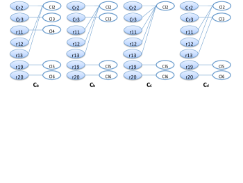
Figure 4: Clustering of $r_{11}-r_{20}$ in Table 2.

Table 5: Element-cluster similarity and SV-index for clusterings in Figure 4. Similarity between an element and its own cluster is in bold and the second-to-highest similarity is in italic. Low $S(e)$ scores are in italic.

	$\mbox{Cl}_{2}$	$\mbox{Cl}_{3}$	$\mbox{Cl}_{4}$	$\mbox{Cl}_{5}$	$\mbox{Cl}_{6}$	$S(e)$
$\mbox{Cr}_{2}$	.9	.5	.5	.5	.5	.44
$\mbox{Cr}_{3}$	.6	1	.5	.5	.5	.4
$r_{11}$	.7	.5	1	.5	.5	.3
$r_{12}$	.99	.5	.95	.5	.5	.05
$r_{13}$	1	.9	.95	.5	.5	.05
$r_{19}$	.5	.5	.5	1	.5	.5
$r_{20}$	.5	.5	.5	.5	1	.5

(a) Cluster ${\cal C}_{a}$.

	$\mbox{Cl}_{2}$	$\mbox{Cl}_{3}$	$\mbox{Cl}_{5}$	$\mbox{Cl}_{6}$	$S(r)$
$\mbox{Cr}_{2}$	.87	.5	.5	.5	.43
$\mbox{Cr}_{3}$	.58	1	.5	.5	.42
$r_{11}$	.79	.5	.5	.5	.37
$r_{12}$	.96	.5	.5	.5	.48
$r_{13}$	.97	.9	.5	.5	.07
$r_{19}$	.5	.5	1	.5	.5
$r_{20}$	.5	.5	.5	1	.5

(b) Cluster ${\cal C}_{b}$.

Cluster adjusting: Although we always assign an element $e$ to the cluster with the highest similarity so $S(e)>0$, the result clustering may still be improved by merging some clusters or moving a subset of elements from one cluster to another. Recall that when $S(e)$ is close to 0 and $a(e)$ is not too small, it indicates that a pair of clusters might be similar and is a candidate for merging. Thus, in cluster adjusting, we find such candidate pairs, iteratively adjust them by merging them or moving a subset of elements between them, and choose the new clustering if it increases the SV-index.

We first describe how we find candidate pairs. Consider element $e$ and assume it is closest to clusters $Cl$ and $Cl^{\prime}$. If $S(e)\leq\theta_{s}$, where $\theta_{s}$ is a threshold for considering merging, we call it a border element of $Cl$ and $Cl^{\prime}$ and consider $(Cl,Cl^{\prime})$ as a candidate pair. We rank the candidates according to (1) how many border elements they have and (2) for each border element $e$, how close $S(e)$ is to 0. Accordingly, we define the benefit of merging $Cl$ and $Cl^{\prime}$ as $b(Cl,Cl^{\prime})=\sum_{e\ is\ a\ border\ of\ Cl\ and\ Cl^{\prime}}(1-S(e))$, and rank the candidate pairs in decreasing order of the benefit.

We next describe how we re-cluster elements in a candidate pair $(Cl,Cl^{\prime})$. We adjust by merging the two clusters, or moving the border elements between the clusters, or moving out the border elements and merging them. Figure 5 shows the four re-clustering plans for a candidate pair. Among them, we consider those that are valid (i.e., a cluster cannot contain more than one satellite but no core) and choose the one with the highest SV-index. When we compute SV-index, we consider only elements in $Cl,Cl^{\prime}$ and those that are second-to-closest to $Cl$ or $Cl^{\prime}$ (their $a(e)$ or $b(e)$ can be changed) such that we can reduce the computation cost. After the adjusting, we need to re-compute $S(e)$ for these elements and update the candidate-pair list accordingly.

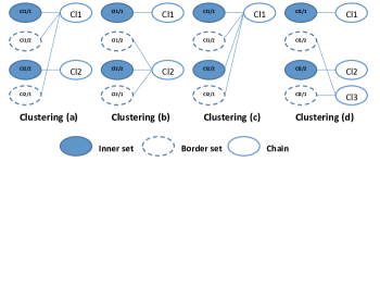
Figure 5: Reclustering plans for $Cl_{1}$ and $Cl_{2}$.

Example 5.4.

Consider adjusting cluster ${\cal C}_{a}$ in Figure 4. Table 5(a) shows similarity of each element-cluster pair and SV-index of each element. Thus, the SV-index is .32.

Suppose $\theta_{s}=.3$. Then, $r_{11}-r_{13}$ are border elements of $\mbox{Cl}_{2}$ and $\mbox{Cl}_{4}$, where $b(\mbox{Cl}_{2},\mbox{Cl}_{4})=.7+.95+.95=2.6$ (there is a single candidate so we do not need to compare the benefit). For the candidate, we have two re-clustering plans, $\{\{r_{11}-r_{13},\mbox{Cr}_{2}\}\}$, $\{\{r_{11}-r_{13}\},\{\mbox{Cr}_{2}\}\}$, while the latter is invalid. For the former (${\cal C}_{b}$ in Figure 4), we need to update $S(e)$ for every element and the new SV-index is $.4$ (Table 5(b)), higher than the original one. $\Box$

The full clustering algorithm Cluster (details in Algorithm 4) goes as follows.

1. Initialize a clustering $\cal C$ and a list $Que$ of candidate pairs ranked in decreasing order of merging benefit. (Lines 1-2).

2. For each candidate pair $(Cl,Cl^{\prime})$ in $Que$ do the following.

   (a) Examine each valid adjusting plan and compute SV-index for it, and choose the one with the highest SV-index. (Line 4).

   (b) Change the clustering if the new plan has a higher SV-index than the original clustering. Recompute $S(e)$ for each relevant element $e$ and move $e$ to a new cluster if appropriate. Update $Que$ accordingly. (Lines 6-16).

3. Repeat Step 2 until $Que=\emptyset$.

Algorithm 4 Cluster($\bf E,\theta_{s}$)

0:  $\bf E$: A set of cores and satellites for clustering.  $\theta_{s}$: Pre-defined threshold for considering merging.

0:  $\cal C$: A clustering of elements in $\bf E$.

1:  Initialize $\cal C$ according to $\bf E$;

2:  Compute $S({\cal C})$ and generate a list $Que$ of candidate pairs;

3:  for each candidate pair $(Cl,Cl^{\prime})\in Que$ do

4:     compute SV-index for its valid re-clustering plans and choose the clustering $\cal C$_max with the highest SV-index;

5:     if $S(\cal C$$)<S(\cal C$${}_{max})$ then

6:        let ${\cal C}={\cal C}_{max}$, $change=true$;

7:        while $change$ do

8:           $change=false$;

9:           for each relevant element $e$ do

10:              recompute $S(e)$;

11:              When appropriate, move $e$ to a new cluster and set $change=true$;

12:              if $S(e)<\theta_{s}$ in the previous or current $\cal C$ then

13:                 update the merging benefit of the related candidate pair and add it to $Que$ or remove it from $Que$ when appropriate;

14:              end if

15:           end for

16:        end while

17:     end if

18:  end for

19:  return  $\cal C$;

Proposition 5.5.

Let $l$ be the number of distinct candidate pairs ever in $Que$ and $|{\bf E}|$ be the number of input elements. Algorithm Cluster takes time $O(l\cdot|{\bf E}|^{2})$. $\Box$

Proof 5.6.

It takes time $O(|{\bf E}|^{2})$ to initialize clustering $\cal C$ and list $Que$. It takes $|{\bf E}|^{2}$ to check each distinct candidate pair in $Que$, where it takes $O(|{\bf E}|)$ to examine all valid clustering plans and select the one with highest SV-index (Step 2(a)), and it takes $O(|{\bf E}|^{2})$ to recompute SV-index for all relevant elements and update $Que$ (Step 2(b)). In total there are $l$ distinct candidate pairs ever in $Que$, thus Cluster takes time $O(l\cdot|{\bf E}|^{2})$.

Note that we first block records according to name similarity and take each block as an input, so typically $|{\bf E}|$ is quite small. Also, in practice we need to consider only a few candidate pairs for adjusting in each input, so $l$ is also small.

Example 5.7.

Continue with Example 5.4 and consider adjusting ${\cal C}_{b}$. Now there is one candidate pair $(\mbox{Cl}_{2},\mbox{Cl}_{3})$, with border $r_{13}$. We consider clusterings ${\cal C}_{c}$ and ${\cal C}_{d}$. Since $S(\cal C$${}_{c})=.37<.40$ and $S(\cal C$${}_{d})=.32<.40$, we keep $\cal C$_b and return it as the result. We do not merge records $\mbox{Cl}_{2}=\{r_{11}-r_{15}\}$ with $\mbox{Cl}_{3}=\{r_{16}-r_{18}\}$, because they share neither phone nor the primary URL. Cluster returns the correct chains. $\Box$

6 Experimental Evaluation

This section describes experimental results on two real-world data sets, showing high scalability of our techniques, and advantages of our algorithm over rule-based or traditional machine-learning methods on accuracy.

Table 6: Statistics of the experimental data sets.

		$\#$Groups		#Singletons
	$\#$Records	(size $>1$)	Group size	(size $=1$)
Random	2062	30	[2, 308]	503
AI	2446	1	2446	0
UB	322	9	[2, 275]	5
FBIns	1149	14	[33, 269]	0
SIGMOD	590	71	[2, 41]	162

6.1 Experiment settings

Data and gold standard: We experimented on two real-world data sets. Biz contains 18M US business listings and each listing has attributes name, phone, URL, location and category; we decide which listings belong to the same business chain. SIGMOD contains records about 590 attendees of SIGMOD’98 and each record has attributes name, affiliation, address, phone, fax and email; we decide which attendees belong to the same institute.

We experimented on the whole Biz data set to study scalability of our techniques. We evaluated accuracy of our techniques on five subsets of data. The first four are from Biz. (1) Random contains 2062 listings from Biz, where 1559 belong to 30 randomly selected business chains, and 503 do not belong to any chain; among the 503 listings, 86 are highly similar in name to listings in the business chains and the rest are randomly selected. (2) AI contains 2446 listings for the same business chain Allstate Insurance. These listings have the same name, but 1499 provide URL “allstate.com”, 854 provide another URL “allstateagencies.com”, while 130 provide both, and 227 listings do not provide any value for phone or URL. (3) UB contains 322 listings with exactly the same name Union Bank and highly similar category values; 317 of them belong to 9 different chains while 5 do not belong to any chain. (4) FBIns data set contains 1149 listings with similar names and highly similar category values; they belong to 14 different chains. Among the listings, 708 provide the same wrong name Texas Farm Bureau Insurance and meanwhile provide a wrong URL farmbureauinsurance-mi.com. Among these four subsets, the latter three are hard cases; for each data set, we manually verified all the chains by checking store locations provided by the business-chain websites and used it as the gold standard. The last “subset” is actually the whole SIGMOD data set. It has very few wrong values, but the same affiliation can be represented in various ways and some affiliation names can be very similar (e.g., UCSC vs. UCSD). We manually identified 71 institutes that have multiple attendees and there are 162 attendees who do not belong to these institutes. Table 6 shows statistics of the five subsets.

Measure: We considered each group as a cluster and compared pairwise linking decisions with the gold standard. We measured the quality of the results by precision ($P$), recall ($R$), and F-measure ($F$). If we denote the set of true-positive pairs by $TP$, the set of false-positive pairs by $FP$, and the set of false-negative pairs by $FN$, then, $P=\frac{|TP|}{|TP|+|FP|}$, $R=\frac{|TP|}{|TP|+|FN|}$, $F=\frac{2PR}{P+R}$. In addition, we reported execution time.

Implementation: We implemented the technique we proposed in this paper, and call it Group. In core generation, for Biz we considered two records are similar if (1) their name similarity is above .95; and (2) they share at least one phone or URL domain name. For SIGMOD we require (1) affiliation similarity is above .95; and (2) they share at least one of phone prefix (3-digit), fax prefix (3-digit), email server, or the addresses have a similarity above .9. We required 2-robustness for cores. In clustering, (1) for blocking, we put records whose name similarity is above .8 in the same block; (2) for similarity computation, we computed string similarity by Jaro-Winkler distance [5], we set $\alpha=.01,\beta=.02,\theta_{th}=.6,p=.8$, and we learned other weights from 1000 records randomly selected from Random data for Biz, and 300 records randomly selected from SIGMOD. We discuss later the effect of these choices.

For comparison, we also implemented the following baselines:

• SameName groups Biz records with highly similar names and groups SIGMOD records with highly similar affiliations (similarity above .95);

• ConnectedGraph generates the similarity graph as
  Group but considers each connected subgraph as a group;

• One-stage machine-learning linkage methods include Partition, Center and Merge [16]; each method computes record similarity by Eq.(3) with learned weights.

• Two-stage method Yoshida [30] generates cores by agglomerative clustering with threshold .9 in the first stage, uses TF/IDF weights for features and applies linear algebra to assign each record to a group in the second stage.

We implemented the algorithms in Java. We used a Linux machine with Intel Xeon X5550 processor (2.66GHz, cache 8MB, 6.4GT/s QPI). We used MySQL to store the data sets and stored the index as a database table. Note that after blocking, we can fit each block of nodes or elements into main memory, which is typically the case with a good blocking strategy.

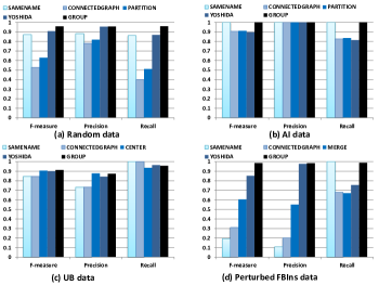
Figure 6: Overall results on Biz data set.

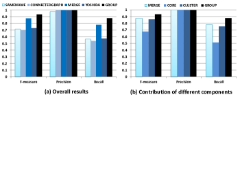
Figure 7: Results on SIGMOD data.

6.2 Evaluating effectiveness

We first evaluate effectiveness of our algorithms. Figure 6 and Figure 7(a) compare Group with the baseline methods, where for the three one-stage linkage methods we plot only the best results. On FBIns, all methods put all records in the same chain because a large number (708) of listings have both a wrong name and a wrong URL. We manually perturbed the data as follows: (1) among the 708 listings with wrong URLs, 408 provide a single (wrong) URL and we fixed it; (2) for all records we set name to “Farm Bureau Insurance”, so removed hints from business names. Even after perturbing, this data set remains the hardest and we use it hereafter instead of the original one for other experiments.

We have the following observations. (1) Group obtains the highest F-measure (above .9) on each data set. It has the highest precision most of the time as it applies core identification and leverages the strong evidence collected from resulting cores. It also has a very high recall (mostly above .95) on each subset because the clustering phase is tolerant to diversity of values within chains. (2) The F-measure of SameName is 7-80% lower than Group. It can have false positives when listings of highly similar names belong to different chains and can also have false negatives when some listings in a chain have fairly different names from other listings. It only performs well in AI, where it happens that all listings have the same name and belong to the same chain. (3) The F-measure of ConnectedGraph is 2-39.4% lower than SameName. It requires in addition sharing at least one value for dominant-value attributes. As a result, it has a lower recall than SameName; it has fewer false positives than SameName, but because it has fewer true positives, its precision can appear to be lower too. (4) The highest F-measure of one-stage linkage methods is 1-94.7% higher than ConnectedGraph. As they require high record similarity, it has similar number of false positives to ConnectedGraph but often has much more true positives; thus, it often has a higher recall and also a higher precision. However, the highest F-measure is still 1-38.7% lower than Group. (5) Yoshida has comparable precision to Group since its first stage is conservative too, which makes it often improve over the best of one-stage linkage methods on Biz dataset where reducing false positives is a big challenge; on the other hand, its first stage is often too conservative (requiring high record similarity) so the recall is 10-34.6% lower than Group, which also makes it perform worse than one-stage linkage methods on Sigmod dataset where reducing false negatives is challenging.

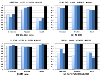
Figure 8: Contribution of different components on Biz.

Contribution of different components: We compared Group with (1) Core, which applies Algorithm CoreIdentification but does not apply clustering, and (2) Cluster, which considers each individual record as a core and applies Algorithm Cluster (in the spirit of [20, 28]). Figure 8 and Figure 7(b) show the results. First, we observe that Core improves over one-stage linkage methods on precision by .1-78.6% but has a lower recall (1.5-34.3% lower) most of the time, because it sets a high requirement for merging records into groups. Note however that its goal is indeed to obtain a high precision such that the strong evidence collected from the cores are trustworthy for the clustering phase. Second, Cluster often has higher precision (by 1.6-77.3%) but lower recall (by 2.5-32.2%) than the best one-stage linkage methods; their F-measures are comparable on each data set. On some data sets (Random, FBIns) it can obtain an even higher precision than Core, because Core can make mistakes when too many records have erroneous values, but Cluster may avoid some of these mistakes by considering also similarity on state and category. However, applying clustering on the results of Cluster would not change the results, but applying clustering on the results of Core can obtain a much higher F-measure, especially a higher recall (98% higher than Cluster on Random). This is because the result of Cluster lacks the strong evidence collected from high-quality cores so the final results would be less tolerant to diversity of values, showing the importance of core identification. Finally, we observe that Group obtains the best results in most of the data sets.

We next evaluate various choices in the two stages. Unless specified otherwise, we observed similar patterns on each data set from Biz and Sigmod, and report the results on Random or perturbed FBIns data, whichever has more distinguishable results.

6.2.1 Core identification

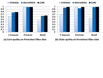
Figure 9: Core identification on perturbed FBIns data.

Core identification: We first compared three core-generation strategies: Core iteratively invokes Screen and Split, OnlyScreen only iteratively invokes Screen, and YoshidaI generates cores by agglomerative clustering [30]. Recall that by default we apply Core. Figure 9 compares them on the perturbed FBIns data. First, we observe similar results of OnlyScreen and Core on all data sets since most inputs to Split pass the $k$-robustness test. Thus, although Screen in itself cannot guarantee soundness of the resulting cores (k-robustness), it already does well in practice. Second, YoshidaI has lower recall in both core and clustering results, since it has stricter criteria in core generation.

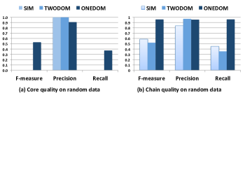
Figure 10: Effect of graph generation on Random data.

Graph generation: We compared three edge-adding strategies for similarity graphs: Sim takes weighted similarity on each attribute except location and requires a similarity of over .8; TwoDom requires sharing name and at least two values on dominant-value attributes; OneDom requires sharing name and one value on dominant-value attributes. Recall that by default we applied OneDom. Figure 10 compares these three strategies. We observe that (1) Sim requires similar records so has a high precision, with a big sacrifice on recall for the cores (0.00025); as a result, the F-measure of the chains is very low (.59); (2) TwoDom has the highest requirements and so even lower recall than Sim for the cores (.00002), and in turn it has the lowest F-measure for the chains (.52). This shows that only requiring high precision for cores with big sacrifice on recall can also lead to low F-measure for the chains.

We also varied the similarity requirement for names and observed very similar results (varying by .04%) when we varied the threshold from .8 to .95.

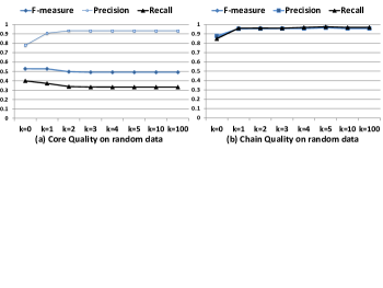
Figure 11: Effect of robustness requirement on Random data.

Robustness requirement: We next studied how the robustness requirement can affect the results (Figure 11). We have three observations. (1) When $k=0$, we essentially take every connected subgraph as a core, so the generated cores can have a much lower precision; those false positives cause both a low precision and a low recall for the resulting chains because we do not collect high-quality strong evidence. (2) When we vary $k$ from 1 to 4, the number of false positives decreases while that of false negatives increases for the cores, and the F-measure of the chains increases but only very slightly. (3) When we continue increasing k, the results of cores and clusters remain stable. This is because setting k=4 already splits the graph into subgraphs, each containing a single v-clique, so further increasing k would not change the cores. This shows that considering $k$-robustness is important, but $k$ does not need to be too high.

6.2.2 Clustering

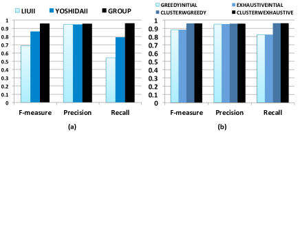
Figure 12: Clustering strategies on Random data.

Clustering strategy: We first compared our clustering algorithm with two algorithms proposed for the second stage of two-stage clustering: LiuII [22] iteratively applies majority voting to assign each record to a cluster and collects a set of representative features for each cluster using a threshold (we set it to 5, which leads to the best results); YoshidaII [30] is the second stage of Yoshida. Figure 12(a) compares their results. We observe that our clustering method improves the recall by 39% over LiuII and by 11% over YoshidaII. LiuII may filter strong evidence by the threshold; YoshidaII cannot handle records whose dominant-value attributes have null values well.

We also compared four clustering algorithms: GreedyInitial performs only initialization as we described in Section 5; ExhaustiveInitial also performs only initialization, but by iteratively conducting matching and merging until no record can be merged to any core; ClusterWGreedy applies cluster adjusting on the results of GreedyInitial, and ClusterWExhaustive applies cluster adjusting on the results of ExhaustiveInitial. Recall that by default we apply ClusterWGreedy. Figure 12(b) compares their results. We observe that (1) applying cluster adjusting can improve the F-measure a lot (by 8.6%), and (2) exhaustive initialization does not significantly improve over greedy initialization, if at all. This shows effectiveness of the current algorithm Cluster.

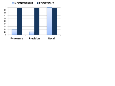
Figure 13: Value weights on perturbed FBIns data.

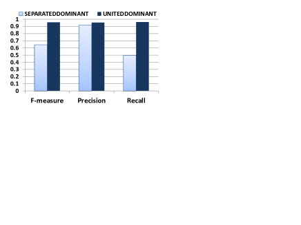
Figure 14: Dominant-value attributes on Random.

Value weight: We then compared the results with and without setting popularity weights for values. Figure 14 compares the results with and without setting popularity weights on perturbed FBIns data. We observe that setting the popularity weight helps distinguish primary values from unpopular values, thus can improve the precision. Indeed, on perturbed FBIns data it improves the precision from .11 to .98, and improves the F-measure by 403%.

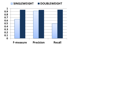
Figure 15: Distinct values on Random data.

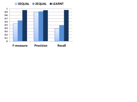
Figure 16: Attribute weights on Random data.

Attribute weight: We next considered our weight learning strategy. We first compared SeparatedDominant, which learns separated weights for different dominant-value attributes, and UnitedDominant (our default), which considers all such attributes as a whole and learns one single weight for them. Figure 14 shows that on Random the latter improves over the former by 95.4% on recall and obtains slightly higher precision, because it penalizes only if neither phone nor URL is shared and so is more tolerant to different values for dominant-value attributes. This shows importance of being tolerant to value variety on dominant-value attributes.

Next, we compared SingleWeight, which learns a single weight for each attribute, and DoubleWeight (our default), which learns different weights for distinct values and non-distinct values for each attribute. Figure 16 shows that DoubleWeight significantly improves the recall (by 94% on Random) since it rewards sharing of distinct values, and so can link some satellite records with null values on dominant-value attributes to the chains they should belong to. This shows importance of distinguishing distinct and non-distinct values.

We also compared three weight-setting strategies: (1) 3Equal considers common-value attributes, dominant-value attributes, and multi-value attributes, and sets the same weight for each of them; (2) 2Equal sets equal weight of .5 for common-value attributes and dominant-value attributes, and weight of .1 for each multi-value attribute; (3) Learned applies weights learned from labeled data. Recall that by default we applied Learned. Figure 16 compares their results. We observe that (1) 2Equal obtains higher F-measure than 3Equal (.64 vs. .54), since it distinguishes between strong and weak indicators for record similarity; (2) Learned significantly outperforms the other two strategies (by 50% over 2Equal and by 76% over 3Equal), showing effectiveness of weight learning. This shows importance of weight learning.

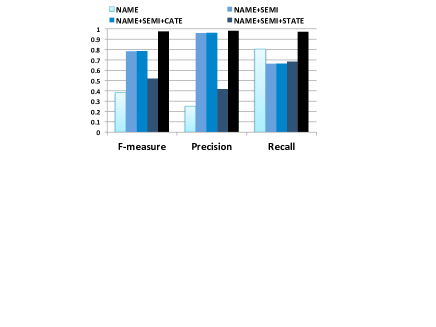
Figure 17: Attribute contribution on perturbed FBIns.

Attribute contributions: We then consider the contribution of each attribute for chain classification. Figure 17 shows the results on the perturbed FBIns data and we have four observations. (1) Considering only name but not any other attribute obtains a high recall but a very low precision, since all listings on this data set have the same name. (2) Considering dominant-value attributes in addition to name can improve the precision significantly and improve the F-measure by 104%. (3) Considering category in addition does not further improve the results while considering state in addition even drops the precision significantly, since three chains in this data set contain the same wrong value on state. (4) Considering both category and state improves the recall by 46% and obtains the highest F-measure.

Robustness w.r.t. parameters: We also ran experiments to test robustness against parameter setting. We observed very similar results when we ranged $p$ from .8 to 1 and $\theta_{th}$ from .5 to .7.

6.3 Evaluating efficiency

Our algorithm finished in 8.3 hours on the whole Biz data set with 18M listings; this is reasonable given that it is an offline process and we used a single machine. Note that simpler methods (we describe shortly) took over 10 hours even for the first stage on fragments of the Biz data set. Also note that using the Hadoop infrastructure can reduce execution time for graph construction from 1.9 hours to 37 minutes; we skip the details as it is not the focus of the paper.

Stage I: It spent 1.9 hours for graph construction and 2.2 minutes for core generation. To test scalability and understand importance of our choices for core generation, we randomly divided the whole data set into five subsets of the same size; we started with one subset and gradually added more. We compared five core generation methods: Naive applies Split on the original graph; Index optimizes Naive by using an inverted index; SIndex simplifies the inverted list by Theorem 4.5; Union in addition merges v-cliques into v-unions by Theorem 4.6; Core (Algorithm 1) in addition splits the input graph by Theorem 4.7. Figure 18(a) shows the results and we have five observations. (1) Naive was very slow. Even though it applies Split rather than finding the max flow for every pair of nodes, so already optimizes by Theorem 4.14, it took 6.8 hours on only 20% data and took more than 10 hours on 40% data. (2) Index improved Naive by two orders of magnitude just because the index simplifies finding neighborhood v-cliques; however, it still took more than 10 hours on 80% data. (3) SIndex improved Index by 41% on 60% data as it reduces the size of the inverted index by 64%. (4) Union improved SIndex by 47% on 60% data; however, it also took more than 10 hours on 80% data. (5) Core improved Union significantly; it finished in 2.2 minutes on the whole data set so further reduced execution time by at least three orders of magnitude, showing importance of splitting. Finally, for graph construction, Figure 18(b) shows the linear growth of the execution time.

Stage II: After core identification we have .7M cores and 17.3M satellites. It spent 6.4 hours for clustering: 1.7 hours for blocking and 4.7 hours for clustering. The long time for clustering is because of the huge number of blocks. There are 1.4M blocks with multiple elements (a core is counted as one element), with a maximum size of 22.5K and an average of 4.2. On only 35 blocks clustering took more than 1 minute and the maximum is 2.5 minutes, but for 99.6% blocks the size is less than 100 and Cluster took less than 60 ms. The average time spent on each block is only 9.6 ms.

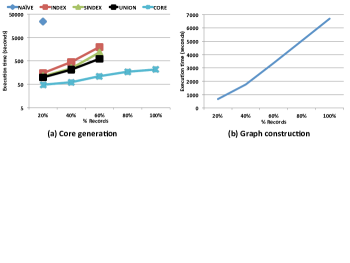
Figure 18: Execution time (we plot only those below 10 hours).

6.4 Summary and discussions

Summary: We summarize our observations as follows.

1. Identifying cores and leveraging evidence learned from the cores is crucial in group linkage.

2. There are often erroneous values in real data and it is important to be robust against them; applying OneDom and requiring $k\in[1,5]$ already performs well on most data sets that have reasonable number of errors.

3. Distinguishing the weights for distinct and non-distinct values, and setting weights of values according to their popularity are critical for obtaining good clustering results.

4. Our algorithm is robust on reasonable parameter settings.

5. Our algorithm is efficient and scalable.

Discussion: In the paper, we present single-machine algorithms to identify groups. Performing such date-intensive tasks on powerful distributed hardwares and service infrastructures has become popular, in particular with the emerging of widely advisable MapReduce programming model [24, 4, 12]. We next discuss possible parallalized solutions of our algorithms in Hadoop infrastructure.

For graph construction, we can proceed in two steps: (1) to create all cliques where nodes sharing the same common-value and a particular dominant-valued attribute are in the same clique, and (2) to find all maximal cliques. In step (1), we first distribute records and map a record $r$ to one or more $<key,value>$ pairs where $key$ is a value on a particular dominant-value attribute of $r$ and $value$ is the value for common-value attribute of $r$ (Mapper). We then find cliques in each block with a particular $key$, and meanwhile keep an inverted list for each block (Reducer). Step (2) takes the output inverted lists and cliques in Step (1) as input. It first uses each entry in the inverted lists as a $<key,value>$ pair to map cliques, so that all cliques that a record $r$ belongs to are mapped into the same block (Mapper). We then find all maximal cliques within each block (Reducer).

To detect cores in the similarity graphs, the algorithm proceeds iteratively. We can use Spark [31], a cluster computing framework to support iterative jobs while retaining the scalability and fault tolerance of MapReduce. For each iteration, we first partition the input graphs into blocks so that each block contains all records of the same maximal connected component (Mapper), and proceed Core within each block in parallel (Reducer). Note that the MapReduce solution may not denominate our single-machine solution that takes only 2.2 minutes, because of the additional overhead of the MapReduce program.

In similar ways, we identify groups as follows. We first partition the input elements (satellites and cores) into blocks so that each block contains elements that may potentially belong to the same group (Mapper), and proceed Cluster within each block in parallel (Reducer).

7 Conclusions

In this paper we studied how to link records to identify groups. We proposed a two-stage algorithm that is shown to be empirically scalable and accurate over two real-world data sets. Future work includes studying the best way to combine record linkage and group linkage, extending our techniques for finding overlapping groups, and applying the two-stage framework in other contexts where tolerance to value diversity is critical.

References

- [1] N. Bansal, F. Chiang, N. Koudas, and F. W. Tompa. Seeking stable clusters in the blogosphere. In VLDB, pages 806–817, 2007.
- [2] O. Benjelloun, H. Garcia-Molina, D. Menestrina, Q. Su, S. E. Whang, and J. Widom. Swoosh: a generic approach to entity resolution. VLDB J., 18(1):255–276, 2009.
- [3] H. Bruhn, R. Diestel, and M. Stein. Menger’s theorem for infinite graphs with ends. J. Graph Theory, 50:199–211, 2005.
- [4] C. Chambers, A. Raniwala, F. Perry, S. Adams, R. R. Henry, R. Bradshaw, and N. Weizenbaum. Flumejava: easy, efficient data-parallel pipelines. In PLDI, pages 363–375, 2010.
- [5] W. W. Cohen, P. Ravikumar, and S. E. Fienberg. A comparison of string distance metrics for name-matching tasks. In IIWEB, 2003.
- [6] D. Dey. Entity matching in heterogeneous databases: A logistic regression approach. Decis. Support Syst., 44:740–747, 2008.
- [7] X. Dong, A. Y. Halevy, and J. Madhavan. Reference reconciliation in complex information spaces. In Proc. of SIGMOD, 2005.
- [8] A. K. Elmagarmid, P. G. Ipeirotis, and V. S. Verykios. Duplicate record detection: A survey. IEEE Trans. Knowl. Data Eng., 19(1):1–16, 2007.
- [9] S. Even and E. R. Tarjan. Network flow and testing graph connectivity. SIAM Journal on Computing, 4(4):507–518, 1975.
- [10] W. Fan, X. Jia, J. Li, and S. Ma. Reasoning about record matching rules. PVLDB, 2(1):407–418, 2009.
- [11] I. P. Fellegi and A. B. Sunter. A theory for record linkage. Journal of the Americal Statistical Association, 64(328):1183–1210, 1969.
- [12] R. L. Ferreira Cordeiro, C. Traina, Junior, A. J. Machado Traina, J. López, U. Kang, and C. Faloutsos. Clustering very large multi-dimensional datasets with mapreduce. In KDD, pages 690–698, 2011.
- [13] L. R. Ford and D. R. Fulkerson. Flows in networks. Princeton University Press, 1962.
- [14] T. Gonzalez. On the computational complexity of clustering and related problems. Lecture Notes in Control and Information Sciences, pages 174–182, 1982.
- [15] S. Guo, X. Dong, D. Srivastava, and R. Zajac. Record linkage with uniqueness constraints and erroneous values. PVLDB, 3(1), 2010.
- [16] O. Hassanzadeh, F. Chiang, H. C. Lee, and R. J. Miller. Framework for evaluating clustering algorithms in duplicate detection. PVLDB, pages 1282–1293, 2009.
- [17] M. A. Hernandez and S. J. Stolfo. Real-world data is dirty: Data cleansing and the merge/purge problem. Data Mining and Knowledge Discovery, 2:9–37, 1998.
- [18] S. Huang. Mixed group discovery: Incorporating group linkage with alternatively consistent social network analysis. International Conference on Semantic Computing, 0:369–376, 2010.
- [19] N. Koudas, S. Sarawagi, and D. Srivastava. Record linkage: similarity measures and algorithms. In SIGMOD, 2006.
- [20] B. Larsen and C. Aone. Fast and effective text mining using linear-time document clustering. In KDD, pages 16–22, 1999.
- [21] P. Li, X. L. Dong, A. Maurino, and D. Srivastava. Linking temporal records. PVLDB, 4(11):956–967, 2011.
- [22] X. Liu, Y. Gong, W. Xu, and S. Zhu. Document clustering with cluster refinement and model selection capabilities. In SIGIR, 2002.
- [23] B. W. On, N. Koudas, D. Lee, and D. Srivastava. Group linkage. In ICDE, pages 496–505, 2007.
- [24] K. Shvachko, H. Kuang, S. Radia, and R. Chansler. The hadoop distributed file system. In MSST, pages 1–10, 2010.
- [25] P. R. Silhouettes. A graphical aid to the interpretation and validation of cluster analysis. Journal of Comp. and Applied Math., 20(1):53–65, 1987.
- [26] J. Sima and S. E. Schaeffer. On the np-completeness of some graph cluster measures. Lecture Notes in Computer Science, 2006.
- [27] S. E. Whang, D. Menestrina, G. Koutrika, M. Theobald, and H. Garcia-Molina. Entity resolution with iterative blocking. In SIGMOD, 2009.
- [28] D. T. Wijaya and S. Bressan. Ricochet: A family of unconstrained algorithms for graph clustering. In DASFAA, pages 153–167, 2009.
- [29] W. E. Winkler. Methods for record linkage and bayesian networks. Technical report, U.S. Bureau of the Census, 2002.
- [30] M. Yoshida, M. Ikeda, S. Ono, I. Sato, and H. Nakagawa. Person name disambiguation by bootstrapping. In SIGMIR, 2010.
- [31] M. Zaharia, M. Chowdhury, M. J. Franklin, S. Shenker, and I. Stoica. Spark: cluster computing with working sets. In HotCloud, 2010.