Substrate-induced Majorana renormalization in topological nanowires

Abstract

We theoretically consider the substrate-induced Majorana localization length renormalization in nanowires in contact with a bulk superconductor in the strong tunnel-coupled regime, showing explicitly that this renormalization depends strongly on the transverse size of the one-dimensional nanowires. For metallic (e.g. Fe on Pb) or semiconducting (e.g. InSb on Nb) nanowires, the renormalization effect is found to be very strong and weak respectively because the transverse confinement size in the two situations happens to be 0.5 nm (metallic nanowire) and 20 nm (semiconducting nanowire). Thus, the Majorana localization length could be very short (long) for metallic (semiconducting) nanowires even for the same values of all other parameters (except for the transverse wire size). We also show that any tunneling conductance measurements in such nanowires, carried out at temperatures and/or energy resolutions comparable to the induced superconducting energy gap, cannot distinguish between the existence of the Majorana modes or ordinary subgap fermionic states since both produce very similar broad and weak peaks in the subgap tunneling conductance independent of the localization length involved. Only low temperature (and high resolution) tunneling measurements manifesting sharp zero bias peaks can be considered to be signatures of Majorana modes in topological nanowires.

I Introduction

Majorana fermions (MF), which were proposed theoretically 80 years ago as real solutions of the Dirac equation in the context of understanding neutrinos Majorana1937 , have recently found their incarnations in solid state systems Read2000Paired ; Kitaev2001Unpaired ; Fu2008Superconducting ; Sau2010Generic as zero-energy localized excitations in topological superconductors (TS). In addition to the defining property of being their own anti-particles, MFs in solid state systems are known to have exotic non-Abelian braiding statistics Read2000Paired , making them of high theoretical interest with a potential application in topological quantum computation Nayak2008Non-Abelian ; DasSarma2015Majorana . While the initial proposals involving exotic materials (e.g. $p$-wave superconductors Read2000Paired ; Kitaev2001Unpaired , $\nicefrac{{5}}{{2}}$-fractional quantum Hall states Read2000Paired , and topological insulators Fu2008Superconducting ) have so far escaped experimental realization, more recent proposals utilizing spin-orbit-coupled semiconductors Sau2010Generic ; Sau2010Non-Abelian ; Lutchyn2010Majorana ; Oreg2010Helical or magnetic adatoms Chung2011Topological ; Duckheim2011Andreev ; Choy2011Majorana ; Nadj-Perge2013Proposal proximity-coupled to $s$-wave superconductors have been the major focus of experimental efforts, with several published works claiming the observation of signatures of MFs in such systems Mourik2012Signatures ; Deng2012Anomalous ; Rokhinson2012fractional ; Das2012Zero-bias ; Churchill2013Superconductor-nanowire ; Finck2013Anomalous ; Nadj-Perge2014Observation . The initial claim of the observation of “Signatures of Majorana Fermions in Hybrid Superconductor-Semiconductor Nanowire Devices” by Mourik et al. Mourik2012Signatures in the InSb/Nb system, following precise theoretical predictions Sau2010Non-Abelian ; Lutchyn2010Majorana ; Oreg2010Helical , was later experimentally replicated by several groups in both InSb/Nb Mourik2012Signatures ; Deng2012Anomalous ; Rokhinson2012fractional ; Churchill2013Superconductor-nanowire and InAs/Al Das2012Zero-bias ; Finck2013Anomalous hybrid structures, giving considerable confidence in the universal nature of the underlying physical phenomena. Despite this apparent experimental success, the identification of the zero-bias peak as a MF is still debated BagretsPRL2012 ; *PikulinNJP2012; more definitive proof, such as signatures of the predicted non-Abelian braiding properties, is yet to be detected as unambiguous evidence for the existence of the Majorana mode Nayak2008Non-Abelian ; DasSarma2015Majorana .

The motivation underlying the semiconductor-superconductor heterostructure Majorana platform Sau2010Non-Abelian is the artificial creation of a spinless low-dimensional (either 2D Sau2010Generic ; Sau2010Non-Abelian or 1D Sau2010Non-Abelian ; Lutchyn2010Majorana ; Oreg2010Helical ) $p$-wave superconductor supporting MFs Kitaev2001Unpaired . The effectively spinless $p$-wave superconductivity residing in the semiconductor serves as the TS here arising from a combination of spin-orbit coupling, spin-splitting, and ordinary $s$-wave superconductivity. The combination of spin-splitting and spin-orbit coupling in the semiconductor allows, under appropriate conditions (of large enough spin-splitting and spin-orbit coupling), ordinary $s$-wave singlet Cooper pairs to tunnel from the superconductor to the semiconductor enabling topological $p$-wave superconductivity with triplet superconducting correlations Liu2015Universal to develop in the semiconductor through proximity coupling. The experimentally relevant topological system has been an InSb Mourik2012Signatures ; Deng2012Anomalous ; Rokhinson2012fractional ; Churchill2013Superconductor-nanowire or InAs Das2012Zero-bias ; Finck2013Anomalous nanowire on a Nb or Al superconducting substrate with the Zeeman spin splitting achieved through the application of an external magnetic field. For the magnetic field larger than a critical value, which is given simply by the proximity-induced superconducting gap in the nanowire (assuming the chemical potential in the nanowire can be taken to be zero), the nanowire becomes an effective TS with zero-energy MFs localized at the wire ends Kitaev2001Unpaired ; Sau2010Non-Abelian ; Lutchyn2010Majorana ; Oreg2010Helical . These zero-energy MFs should lead to zero-bias conductance peaks (ZBCP) in the tunneling conductance measurement Sau2010Non-Abelian , and the experimental observation Mourik2012Signatures ; Churchill2013Superconductor-nanowire ; Das2012Zero-bias ; Finck2013Anomalous of such field-induced ZBCP has been taken as evidence for the existence of MFs in these topological nanowires.

Typically, these MFs are localized near the ends of the wire with a finite Majorana localization length $\xi$ which equals the superconducting coherence length in the topological nanowire. When the wire length $L\gg\xi$, the two MFs at the two ends of the wire are considered to be in the topologically exponential protection regime with the MF wavefunction falling off as $e^{-x/\xi}$ along the wire (modulo some oscillations not of particular interest here Cheng2009Splitting ; Cheng2010Stable ; DasSarma2012Splitting ). The MF is a well-defined zero-energy non-Abelian mode only in this exponentially protected ($L\gg\xi$) regime. By contrast, for short wires or long coherence length (i.e. $L<\xi$), the two end MFs hybridize, producing split peaks shifted away from zero energy (and these split peaks represent fermionic subgap states rather than MFs), and the topological protection no longer applies. It is only when the Majorana splitting is exponentially small (i.e. $L\gg\xi$), the nanowire system can be considered to be topological DasSarma2015Majorana . Thus, the quantitative magnitude of $\xi$ (or more precisely the dimensionless length ratio $L/\xi$) is a key ingredient in the physics of MFs. We note that the localized zero-energy MF bound states are also often called the Majorana modes, and we use the terminology Majorana fermions and Majorana modes interchangeably in this paper to mean the same zero-energy MF subgap localized TS excitations in a spinless p-wave superconductor. The current experimental MF search is mostly focused on looking for subgap zero-bias tunneling conductance peaks associated with these localized zero-energy Majorana modes – ideally, the ZBCP should have the quantized value of $2e^{2}/h$, but experimentally the ZBCPs observed so far have actual conductance values factors of 10 ($10^{4}$) lower in semiconductor nanowires Mourik2012Signatures ; Das2012Zero-bias ; Churchill2013Superconductor-nanowire (ferromagnetic nanowires Nadj-Perge2014Observation ). Finite temperature, finite wire length, finite tunnel barrier, finite experimental resolution, unwanted fermionic subgap states, and possible inelastic processes conspire together to suppress the experimental ZBCP strength, and this non-observation of perfect ZBCP quantization, which is much more severe in the ferromagnetic nanowires than in semiconductor systems, remains an open question in the subject.

The MF localization length (or equivalently the TS coherence length) $\xi$ is often assumed to be given by the standard superconducting coherence length formula, $\xi\sim v_{F}/\Delta$, where $v_{F}$ and $\Delta$ are respectively the Fermi velocity and the induced TS gap in the nanowire. This superconducting coherence length formula is certainly appropriate for MF localization if the nanowire can be considered an isolated spinless $p$-wave superconductor with the Majorana modes localized at the wire ends (which serve as the defects localizing the MFs). But in the experimentally relevant situation the nanowire is not isolated, it is in fact in contact with (or lying on top of) a superconducting substrate which provides the necessary proximity effect to produce the topological system in conjunction with spin-orbit coupling and spin splitting. The question therefore arises whether the MF localization length formula is modified from the simple coherence length formula, or equivalently, whether the Fermi velocity and/or the appropriate nanowire superconducting gap are renormalized by the substrate. This issue was in fact discussed by Sau et al. Sau2010Robustness and Stanescu et al. Stanescu2010Proximity some years ago in the context of 2D sandwich structures involving semiconductor/superconductor and topological-insulator/superconductor heterostructures, and very recently by Peng et al. Peng2014Strong in the context of 1D ferromagnetic nanowire on superconductor hybrid structures used in the recent Princeton STM experiment Nadj-Perge2014Observation . (The actual system theoretically considered by Peng et al. Peng2014Strong is in fact a helical magnetic adatom chain, not a ferromagnetic chain, on a superconducting substrate.) In the first part of the current work, we theoretically study the MF localization question in depth for 1D topological nanowire hybrid systems, discussing the substrate-induced MF renormalization for both semiconductor and ferromagnetic nanowires on an equal footing, comparing and contrasting the two situations. In particular, we address the important issue of how it might be possible that Majorana localization length could be strongly (weakly) renormalized in ferromagnetic (semiconductor) nanowire systems studied in different laboratories.

Recently, it has been proposed that the three ingredients for the semiconductor nanowire proposal, i.e. superconductivity, magnetization, and spin-orbit coupling, can be realized in ferromagnetic nanowires deposited on a spin-orbit coupled superconductor. Experimental evidence in the form of a weak and broad zero-bias peak seems to provide some support to this hypothesis Nadj-Perge2014Observation . Several theoretical calculations Nadj-Perge2013Proposal ; Hui2015Majorana ; Dumitrescu2014Majorana ; Li2014Topological ; HeimesNJP2015 have shown that as a matter of principle Majorana modes can emerge in ferromagnetic wires in superconductors, as had been suggested in more mesoscopic geometries Chung2011Topological ; Duckheim2011Andreev ; Takei2012Microscopic ; Wang2010Interplay . Motivated by earlier STM works Yazdani1997Probing ; Ji2008High-Resolution , some of the theoretical works Choy2011Majorana ; Pientka2013Topological ; Kim2014Helical ; HeimesNJP2015 have modeled the system to be a chain of magnetic atoms [i.e. Yu-Shiba-Rusinov (YSR) impurities] on the superconductor surface, with no direct hopping between the impurity orbitals. This class of proposals supports MFs only in a limited parameter regime Brydon2015Topological ; Peng2014Strong . Although the YSR limit and the ferromagnetic nanowire limit are the two extreme crossover regimes (tuned by very weak and very strong inter-site hopping in the nanowire, respectively) of the same underlying Hamiltonian (i.e. there is no quantum phase transition separating them, it is simply a hopping-induced crossover from the YSR regime to the ferromagnetic wire regime as hopping increases), the TS properties in the two limits are very different. In the YSR limit, considerable fine-tuning of the chemical potential is necessary in order to achieve TS and MF Brydon2015Topological ; HeimesNJP2015 , whereas the TS with localized MF arise generically without any fine-tuning in the ferromagnetic nanowire limit of strong hopping. Thus, any possible generic existence of MF in the magnetic adatom chain on superconducting substrates is more natural in the ferromagnetic wire limit Hui2015Majorana ; Dumitrescu2014Majorana rather than in the YSR limit. Therefore, considering the system as a ferromagnetic wire in proximity to a superconductor is the natural way to understand the zero-bias conductance. This puts the ferromagnetic chain and the semiconductor nanowire topological systems on an equal footing with the only difference being that in the semiconductor wire (the ferromagnetic chain) case the spin-splitting arises from an externally applied magnetic field (an intrinsic ferromagnetic exchange splitting). However, in the semiconductor nanowire proposals Lutchyn2010Majorana ; Oreg2010Helical the decay length of the Majorana is typically found to be comparable to the bulk coherence length in the superconductor. This also seems to be a common feature in the simulations of the ferromagnetic nanowire systems so far since the substrate-induced renormalization of the nanowire parameters is not included in the theory, thus considering the nanowire to be effectively isolated Nadj-Perge2013Proposal ; Hui2015Majorana ; Dumitrescu2014Majorana . On the other hand, it was noted that YSR bound states in STM experiments appeared to show a much shorter decay length than the coherence length Yazdani1997Probing ; Ji2008High-Resolution . Based on this, it was conjectured Dumitrescu2014Majorana that the Majorana modes might appear to be confined to length-scales shorter than the coherence length because of the delocalization of the wavefunction into the bulk superconductor. Very recent work using a spin-helical adatom chain model Peng2014Strong has shown how this substrate-induced renormalization mechanism may suppress the coherence length, possibly leading to a short MF localization length in a magnetic chain on a superconductor which is very strongly tunnel-coupled to the magnetic chain, even if the topological superconducting gap is very small. Anomalously short Majorana localization lengths were numerically demonstrated for similar models in Refs. Li2014Topological and HeimesNJP2015 . Whether such a scenario applies to the actual experimental situation of Ref. Nadj-Perge2014Observation is currently unknown.

The actual MF localization length question is of great importance to the experimental observations in Nadj-Perge2014Observation since the estimated TS gap in the Fe adatom chains on Pb substrates studied therein is very small ($\sim 0.1\,{\rm meV}$) leading to a rather long coherence length (or equivalently MF localization length) of $>100\,{\rm nm}$ (assuming no substrate-induced renormalization) which would be much larger than the typical length of the adatom chains ($5-50\,{\rm nm}$) used in Ref. Nadj-Perge2014Observation . In such a situation, the TS system is not in the exponentially protected regime at all, and the two end MFs should hybridize strongly leading to ordinary uninteresting fermionic states at high energies. Thus, to the extent the observations in Nadj-Perge2014Observation manifest MF features, one must understand how the very long TS coherence length (i.e. the MF localization length) associated with the small induced superconducting gap can be consistent with the existence of isolated (i.e. non-hybridized) MFs in a system where the wire length is shorter than the localization length. (This conceptually problematic situation does not seem to arise in the semiconductor TS systems Mourik2012Signatures ; Deng2012Anomalous ; Rokhinson2012fractional ; Das2012Zero-bias ; Churchill2013Superconductor-nanowire ; Finck2013Anomalous since the wire length ($>1\,{\rm\mu m}$) is typically much larger than the MF localization length ($\sim 10\,{\rm nm}$) in the semiconductor nanowire systems— in fact, systematic experimental efforts appeared to have observed the predicted Majorana hybridization effect in the semiconductor nanowires in the regime of long MF localization length induced by a large external magnetic field Churchill2013Superconductor-nanowire ; Finck2013Anomalous .) If the observed subgap conductance features in Ref. Nadj-Perge2014Observation are indeed implying the existence of MFs in the underlying ferromagnetic nanowire, as has been concluded Nadj-Perge2014Observation , then it is imperative that a clear theoretical understanding is developed for why the TS coherence length being much larger than the topological wire length is not a problem. One possible way out of this quandary, suggested by Peng et al. Peng2014Strong using a helical magnetic chain model, is a strong suppression of the MF localization length by the substrate so that the $L\gg\xi$ condition is still satisfied because the TS coherence length is renormalized by the substrate. This solution comes with the caveat that that the strongly localized MF is accompanied by a power-law tail Pientka2013Topological , which extends to the coherence length of the bulk superconductor. So while the localization length appears to be reduced on length-scales where the splitting is measurable in tunneling, it is not clear that this suppression significantly aids the splitting problem for quantum information purposes because of the power-law tail. We emphasize that it is not clear at all at this stage that the condition (in particular, very strong tunnel coupling between the substrate and the chain) for such strong substrate-induced renormalization of the MF localization length is actually operational in the experiment of Ref. Nadj-Perge2014Observation , but the possibility of the substrate-induced suppression of the MF localization length must be taken seriously since it provides a way forward for future experiments to test this hypothesis as a possible resolution of the long TS coherence length conundrum, e.g., by studying the MF hybridization or splitting systematically as a function of the dimensionless ratio $\xi/L$ by changing $L$ in a controlled manner.

The possibility that the MF localization length is strongly suppressed by the substrate immediately brings up the question of whether such a substrate-induced renormalization phenomenon is also operational in the semiconductor TS systems and, if so, the possible implications for the semiconductor MF experiments Mourik2012Signatures ; Deng2012Anomalous ; Rokhinson2012fractional ; Das2012Zero-bias ; Churchill2013Superconductor-nanowire ; Finck2013Anomalous which have so far been simply interpreted on the basis of the standard $\xi\sim v_{F}/\Delta$ formula with no substrate-induced coherence length suppression. The corresponding renormalization question for semiconductor-superconductor 2D hybrid structures was studied in depth in Refs. Stanescu2010Proximity ; Peng2014Strong , and here we generalize the theory to 1D semiconductors and ferromagnetic metals in proximity to bulk superconductors. One possible reconciliation for why the ferromagnetic (semiconductor) nanowire MF localization length is strongly (not) renormalized by the substrate is simply by assuming that the ferromagnetic adatoms (semiconductor wire) are (are not) strongly tunnel-coupled to the substrate superconductor, but we want to avoid such ad hoc assumptions. One question we address in the first part of the paper is how different the substrate-induced Majorana localization length renormalization can be in metallic and semiconductor TS nanowires assuming essentially identical conditions to be prevailing for the substrate properties (including equivalently strong tunnel coupling of the wire to the substrate) in both cases.

In this paper, we discuss in general the localization length of Majorana modes in proximity-induced superconductors. To set a context, we start by discussing the localization length of Majorana modes in the Kitaev chain Kitaev2001Unpaired in various parameter regimes finding that depending on parameter values the localization length can vary from being of the order of a lattice spacing to more than many hundreds of lattice spacings as is typical for the coherence length in ordinary superconductors. Realizations of such Kitaev chains where the Majorana localization length is of the order of several lattice sites have been proposed in quantum dot arrays Sau2012Realizing , and therefore, in principle, the variation in the MF localization properties can be tested in the linear quantum dot arrays by suitably tuning the dot parameters. Following this, we explicitly consider the proximity effect of the bulk superconductor with a goal to understanding the length-scale problem for ferromagnetic nanowires in proximity to spin-orbit coupled superconductors as used in the experiment of Ref. Nadj-Perge2014Observation . While the superconducting proximity effect is simply modeled by a pairing potential in most papers on the subject, a more microscopic consideration Sau2010Robustness suggests that the proximity effect should be represented by a non-local frequency-dependent self-energy

$$\Sigma\left(\omega;\bm{r},\bm{r}^{\prime}\right)=T\left(\bm{r}\right)G_{SC}\left(\omega;\bm{r},\bm{r}^{\prime}\right)T\left(\bm{r}^{\prime}\right)^{\dagger},$$ (1)

where the matrix $T$ represents the hopping between the nanowire and the superconductor, and $G_{SC}(\omega;\bm{r},\bm{r}^{\prime})$ is the Green function of the superconductor. By approximating the Green function by that of a bulk $s$-wave superconductor, we show below that the local part of the self-energy has the form of

$$\Sigma\left(\omega;\bm{r},\bm{r}\right)\sim-\frac{\Gamma\omega}{\Delta_{SC}}\hat{\tau}_{0}+\Gamma\hat{\tau}_{x},$$ (2)

where $\Gamma$ is the parameter determining the strength of the superconducting proximity coupling in the nanowire. As we argue in Sec. III.5, based on a microscopic derivation, the proximity parameter $\Gamma\sim(R/a)^{-3}E_{F}$, where $a\sim 0.5\,{\rm nm}$ and $E_{F}\sim 1\,{\rm eV}$ are respectively a length scale on the order of the lattice constant and the Fermi energy in the superconductor, and $R$ is the radius of the nanowire. In mesoscopic semiconductor nanowire geometries $R\sim 20{\rm nm}$ leading to $\Gamma\sim 0.01{\rm meV}\ll\Delta_{SC}$, and this fits into the simple picture for the proximity effect where retardation effects associated with the frequency dependence in Eq. (2) may be ignored. Atomistic ferromagnetic wires Nadj-Perge2014Observation are qualitatively different since $R\sim 0.5{\rm nm}$ for these wires and the estimated $\Gamma\sim 1{\rm eV}$. This clearly puts the analysis in the regime $\Gamma\gg\Delta_{SC}$, which is the strongly renormalized limit Sau2010Robustness . Establishing this key difference between the MFs in semiconductor and metallic nanowires (i.e. the MF localization length is strongly renormalized in one, but not in the other, due to substrate renormalization arising from retardation effects in the proximity self-energy function) is a main goal of this paper. While it might appear that a proximity effect of $\Gamma\gg\Delta_{SC}$ in the ferromagnetic nanowire system would produce an $s$-wave pairing in the nanowire that is much greater than $\Delta_{SC}$ in contradiction with experiment, the frequency dependence of the self-energy, where $\Gamma$ enters as a parameter, ensures that the $s$-wave pairing in this case is $\Delta_{0}\sim\frac{\Gamma\Delta_{SC}}{\Delta_{SC}+\Gamma}\sim\Delta_{SC}$, which is much less than $\Gamma$. Therefore, it is clear that the full frequency-dependent self-energy is critical to get the physics correct Sau2010Robustness .

We present calculations of the local density of states for the ferromagnetic nanowire in proximity to a spin-orbit coupled superconductor. We find that the frequency dependence introduces renormalization of all microscopic parameters in a way which drastically reduces the coherence length in the ferromagnetic nanowire, in contrast to the semiconductor nanowire MFs where the standard definition for the coherence length applies with little renormalization by the substrate. After establishing that the MF localization in the ferromagnetic nanowire system could indeed be very short in spite of the induced topological superconducting gap being very small, we consider the actual experimental situation Nadj-Perge2014Observation where the MF observation in a Fe chain on a superconducting Pb substrate has been claimed in an STM study. At first, the very small induced gap ($\sim 100\,{\rm\mu eV}$) in the experiment seems to indicate a very long MF localization length much larger than the length of the Fe chains, casting serious doubt on the experimental interpretation of lattice-scale MF localization in the system. Peng et al. Peng2014Strong , however, provided a way out of this puzzle by showing that, assuming the Pb-Fe tunnel coupling is strong, it is possible for the MF localization length to be short in spite of the induced gap being small within their helical chain model. In the current work, we go beyond the analysis in Ref. Peng2014Strong by showing that this renormalization is a generic feature of chain TS platforms. Moreover, we directly address the question of why such effects are weak in the semiconductor nanowire, revealing the key role of mesoscopic vs microscopic geometry in determining the substrate coupling strength. This provides a clearer understanding of the relationship between these the superficially different chain and nanowire TS platforms.

In the second part of the paper, we address the issue of energy localization of the Majorana zero mode in the recent ferromagnetic wire STM experiment Nadj-Perge2014Observation . Apart from spatial localization, another peculiar feature of the Majorana modes in the ferromagnetic nanowire experiment relates to the broadening of the spectrum in the energy domain. This feature of the experiment Nadj-Perge2014Observation results from the high temperatures ($T=1.4\,{\rm K}$) at which the experiment is carried out comparable to the induced gap ($\sim 0.1\,{\rm meV}$) itself. Such high temperatures limit the energy resolution of the STM, thus compromising the claim of the MF observation in Ref. Nadj-Perge2014Observation . The Majorana mode must be localized both spatially and spectrally, i.e., the MF must be a well-defined zero energy excitation (in addition to being spatially localized at the wire ends) which becomes problematic at high temperatures where the zero mode hybridizes with the above-gap fermionic particle-hole excitations, thus completely losing its non-Abelian Majorana character. The energy localization property is independent of the spatial localization aspect, and both properties must be satisfied for a system to have MF modes. It has recently been shown Dumitrescu2014Majorana that at such a high temperature the MF signature manifested in the tunneling experiment is diffuse over an energy range larger than the gap itself, and as such, the issue of MF localization becomes moot because of the participation of other states. In the second part of our paper, we show that such broad and diffuse zero bias tunneling conductance peak could arise from subgap non-MF states which may generically be present in the system due to disorder. Thus, although the MF may indeed be strongly localized in the ferromagnetic nanowire system, tunneling experiments at temperatures (and instrumental resolution) comparable to the gap energy cannot distinguish between MF features and ordinary (non-MF) subgap state features. Only future experiments carried out at much lower temperatures can therefore settle the question of what is being observed in the experiment of Ref. Nadj-Perge2014Observation . At much lower temperatures, however, the strongly localized nature of the MFs in the ferromagnetic nanowires will come into play in a dramatic fashion, leading to a strong zero bias conductance peak in long wires and clearly split zero bias peaks in short wires, thus definitively establishing the existence (or not) of MFs in the ferromagnetic wire - superconductor hybrid structure. On the other hand, if the physics of substrate-induced MF localization length suppression is not playing any role in the ferromagnetic adatom chains (as it is not in semiconductor nanowires) on superconducting substrates, then at temperatures much lower than the induced gap, the subgap zero bias peak, if it is indeed arising from TS physics, should simply disappear completely since the MF localization length in such an unrenormalized situation would be much larger than the ferromagnetic adatom chain length one can fabricate on superconducting substrates at the present time. Thus, lowering (and improving) experimental temperature (instrumental resolution) is the key to settling the question of whether MFs have indeed been observed in the experiments carried out in Ref. Nadj-Perge2014Observation . Since the state of the arts low-temperature STM experiments are routinely carried out at $\sim 100\,{\rm mK}$ or below Firmo2013Evidence ; *Allan2013Imaging; *ZhouNatPhys2013 (a temperature regime accessible since the early 1990s HessPRL1990 ), we urge future STM low temperature experiments ($<300\,{\rm mK}$) in Fe chains on superconducting Pb substrates to settle the important question of the existence or not of MFs in this system.

At this stage all one can say is that while Majorana modes do not show any basic inconsistencies with experiment, the broad features in the experiment Nadj-Perge2014Observation could also be consistent with accidental fermionic non-MF subgap states. In fact, the possibility that the observed subgap tunneling conductance structure in the experiment of Ref. Nadj-Perge2014Observation arises purely from a type of YSR bound states, rather than MF states, has been suggested recently Sau2015Bound . In fact, the possibility that the observed Nadj-Perge2014Observation broad and weak zero bias feature arises from completely different physics Sau2015Bound ; Kontos2001Inhomogeneous ; *Fauchere1999Paramagnetic nothing to do with Majorana fermions cannot be ruled out at this stage.

II Majorana decay length in the Kitaev Chain

Let us first consider the prototypical and simplest model of a TS supporting Majorana end modes, the so-called Kitaev chain. This is a one-dimensional tight-binding model of spinless fermions with $p$-wave pairing, described by the Hamiltonian

$$H_{w} =-t\sum_{j}\left(a_{j}^{\dagger}a_{j+1}+{\rm h.c.}\right)-\mu\sum_{j}a_{j}^{\dagger}a_{j}$$

$$+\Delta_{p}\sum_{j}\left(a_{j}a_{j+1}+{\rm h.c.}\right)\,,$$ (3)

where $t$ is the hopping, $\mu$ the chemical potential, and $\Delta_{p}$ is the pairing potential. As shown by Kitaev Kitaev2001Unpaired , this model supports unpaired Majorana modes at its boundaries for $\left|\mu\right|<2\left|t\right|$, with a MF localization length that is given by

$$\xi=\max_{\lambda=\pm 1}\left(\left|\textrm{log}\left|\frac{\lambda\sqrt{\mu^{2}-4t^{2}+4\Delta_{p}^{2}}-\mu}{2\left(t+\left|\Delta_{p}\right|\right)}\right|\right|\right)^{-1}.$$ (4)

We plot the localization length in Fig. 1 as a function of the hopping amplitude for different values of $\mu$. Note that $\xi$ is defined only for $\left|t\right|>\left|\mu\right|/2$, where the system is in the topologically non-trivial regime with a Majorana mode at each end. At $\left|t\right|=\left|\mu\right|/2$ the localization length diverges, indicating a topological phase transition into the topologically trivial regime at $|t|<|\mu|/2$.

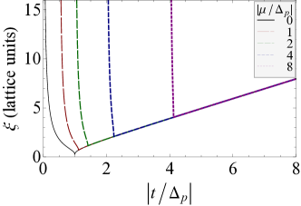
Figure 1: MF localization length $\left(\xi\right)$ given by Eq. (4) as a function of dimensionless hopping strength ($|t/\Delta_{p}|$) for various values of the chemical potential ($|\mu/\Delta_{p}|$). For $|t|<|\mu|/2$ the system is in the non-topological phase without Majorana fermions, and $\xi$ is undefined in this regime. $\xi$ diverges at $|t|=|\mu|/2$, indicating the topological phase transition. For $|t|\gg|\mu|$, $\xi$ is well-approximated by $|t/\Delta_{p}|$, which is the standard coherence length formula for superconductors.

There are two special limits of interest. At the special point $\mu=0$ and $|t|=|\Delta_{p}|$, the localization length vanishes and the Majorana is localized precisely at the end site of the chain Kitaev2001Unpaired . We emphasize that in this fine-tuned case the localization of the Majorana is completely independent of the size of the energy gap, providing a concrete example of a situation where a small gap could in principle also be associated with a small localization length. The other situation of interest is the physically realistic limit $|t|\gg|\Delta_{p}|$, where the bandwidth far exceeds the superconducting gap Sengupta2001Midgap . Here the localization length $\xi$, expressed to lowest order in $\Delta_{p}$, reproduces the familiar form of a superconducting coherence length as discussed in the Introduction,

$$\xi=\left|\frac{t}{\Delta_{p}}\right|=\frac{v_{F}}{2E_{{\rm gap}}},$$ (5)

where $E_{{\rm gap}}=|\Delta_{p}|(1-\mu^{2}/4t^{2})^{1/2}$ and $v_{F}=2|t|(1-\mu^{2}/4t^{2})^{1/2}$ are the spectral gap and Fermi velocity, respectively. Since $|t|\gg|\Delta_{p}|$, the localization length $\xi\gg 1$ and the Majorana decay length is parametrically larger than the lattice constant (taken to be the unit of length here). On the other hand, it is clear that if for some reasons one can realize a Kitaev chain with $\left|t\right|\sim\left|\Delta_{p}\right|$, as has been proposed for a quantum dot array Sau2012Realizing , then the MF decay length is of order a few lattice sites only, qualitatively similar to the fine-tuned case.

III Substrate-Induced Renormalization of the Topological Wire

We now turn to the physical realization Sau2010Non-Abelian ; Lutchyn2010Majorana ; Oreg2010Helical ; Lutchyn2011Search ; Brydon2015Topological ; Hui2015Majorana ; Dumitrescu2014Majorana ; Li2014Topological ; Peng2014Strong ; HeimesNJP2015 of TS in a ferromagnetic nanowire in contact with a bulk $s$-wave superconductor. We note that the minimal model for the ferromagnetic wire proximity-coupled to a superconductor Hui2015Majorana ; Dumitrescu2014Majorana ; Takei2012Microscopic , as used in Ref. Nadj-Perge2014Observation , is formally the same as the corresponding semiconductor nanowire TS system introduced in Refs. Sau2010Non-Abelian ; Lutchyn2010Majorana ; Oreg2010Helical ; Lutchyn2011Search with the only constraint being that the spin-splitting is arising from intrinsic exchange splitting in the ferromagnetic system whereas it is induced as a Zeeman splitting by an externally applied magnetic field in the semiconductor case. This has already been pointed out by Dumitrescu et al. Dumitrescu2014Majorana . The presence of spin-orbit coupling and spin-splitting along with proximity-induced superconductivity enables us to avoid the fermion doubling theorem, leading to topological (effectively spinless p-wave) superconductivity in the wire.

III.1 Self-Energy

The normal state of the superconductor is characterized by strong ${\bf L}\cdot{\bf S}$ spin-orbit coupling. Furthermore, two orbitals of different parity contribute to the states near the Fermi surface, which we label as $s$ and $p\equiv p_{z}$, respectively. This is not essential for our theory (for example, we could also choose three distinct $p$-wave orbitals), but makes the following arguments more transparent; indeed, the details of the electronic structure of the superconductor are not important for our analysis, which relies on symmetry considerations. Although spin itself is not a good quantum number in the presence of spin-orbit coupling, we can label the doubly-degenerate states by a pseudospin index $\varsigma=\pm 1$, which transforms like a spin under inversion and time-reversal. Assuming only a single band crosses the Fermi surface, the general expression for these states is

$$\left|\bm{k},\varsigma\right\rangle=\sum_{\sigma=\uparrow,\downarrow}\left[B_{s,\varsigma\sigma}\left(\bm{k}\right)\left|s,\bm{k},\sigma\right\rangle+B_{p,\varsigma\sigma}\left(\bm{k}\right)\left|p,\bm{k},\sigma\right\rangle\right],$$ (6)

where $B_{s,\varsigma\sigma}\left(\bm{k}\right)$ and $B_{p,\varsigma\sigma}\left(\bm{k}\right)$ are the coefficients of the $s$- and $p$-wave orbitals, respectively. Regarding the coefficients in Eq. (6) as $2\times 2$ matrices in $\varsigma-\sigma$ space, one can derive a number of conditions. First, the normalization of the states in Eq. (6) requires that

$$\hat{s}_{0}={B_{s}^{*}\left(\bm{k}\right)B_{s}^{T}\left(\bm{k}\right)+B_{p}^{\ast}\left(\bm{k}\right)B_{p}^{T}\left(\bm{k}\right).}$$ (7)

From inversion and time-reversal symmetries we deduce that

$$B_{s}\left(\bm{k}\right)=B_{s}\left(-\bm{k}\right)=\hat{s}_{y}B_{s}^{*}\left(-\bm{k}\right)\hat{s}_{y}\,,$$ (8a)

$$B_{p}\left(\bm{k}\right)=-B_{p}\left(-\bm{k}\right)=\hat{s}_{y}B_{p}^{*}\left(-\bm{k}\right)\hat{s}_{y}\,.$$ (8b)

In these equations $\hat{s}_{\mu}$ are Pauli matrices in the $\varsigma-\sigma$ space. We additionally require that the pseudospin index behaves like a spin under mirror reflection in the planes perpendicular to the three Cartesian axes:

$$B_{s}\left(\bm{k}\right) = \hat{s}_{\mu}B_{s}\left({\cal M}_{\mu}\bm{k}\right)\hat{s}_{\mu}\,,\quad\mu=x,y,z\,,$$ (9a)

$$B_{p}\left(\bm{k}\right) = \begin{cases}\hat{s}_{\mu}B_{p}\left({\cal M}_{\mu}\bm{k}\right)\hat{s}_{\mu}&\mu=x,y\\ -\hat{s}_{\mu}B_{p}\left({\cal M}_{\mu}\bm{k}\right)\hat{s}_{\mu}&\mu=z\end{cases}$$ (9b)

where ${\cal M}_{\mu}$ are reflection operators for the plane perpendicular to the $\mu$-axis.

In the pseudospin basis the bulk Green function of the superconductor is written as

$$G_{SC}\left(\omega;\bm{k}\right)=\frac{\omega\hat{\tau}_{0}+\xi_{\bm{k}}\hat{\tau}_{z}+\Delta_{SC}\hat{\tau}_{x}}{\omega^{2}-\xi_{\bm{k}}^{2}-\Delta_{SC}^{2}},$$ (10)

where $\hat{\tau}_{\mu}$ are Pauli matrices in the particle-hole basis, $\xi_{\bm{k}}$ is the dispersion in the superconductor, and $\Delta_{SC}$ is the gap. The nanowire is placed on the $(001)$ surface of the superconductor. The tunneling between the two systems is described by a superconductor-nanowire hopping term

$$H_{{\rm tun}}=\sum_{n\sigma}\left[a_{n\sigma}^{\dagger}\left(t_{s}s_{n\sigma}+t_{p}p_{n\sigma}\right)+{\rm h.c.}\right],$$ (11)

where $a_{n\sigma}^{\dagger}$ creates an electron with spin $\sigma$ at site $n$ on the nanowire, and $s_{n\sigma}$ and $p_{n\sigma}$ are annihilation operators of the orbitals of the superconductor. Only nearest-neighbor hopping is allowed. We remark here that a local breaking of inversion symmetry along $z$ is required to generate non-zero $t_{p}$ which couples the nanowire sites to the $p$-orbital in the superconductor. Without loss of generality, we take $t_{s}$ and $t_{p}$ to be real.

The tunneling matrix $T$, which appears in the self-energy of the nanowire [Eq. (1)], necessarily includes a transformation between the real-spin basis of the nanowire and the pseudospin basis of the superconductor. It is written

$$T = \left(\begin{array}[]{cc}t_{s}B_{s}^{T}+t_{p}B_{p}^{T}&0\\ 0&-t_{s}B_{s}^{T}-t_{p}B_{p}^{T}\end{array}\right).$$ (14)

With $G_{SC}$ and $T$, the self-energy $\Sigma$ can be readily computed as

$$\Sigma\left(\omega;\bm{r},\bm{r}^{\prime}\right) = \int\frac{d^{3}k}{\left(2\pi\right)^{3}}e^{i\bm{k}\cdot\left(\bm{r}-\bm{r}^{\prime}\right)}T\left(\bm{k}\right)G_{SC}\left(\omega;\bm{k}\right)T\left(\bm{k}\right)^{\dagger}$$ (15)

$$= \left(1-Z\right)\omega+Zt\hat{\tau}_{z}+Z\bm{\lambda}\cdot\hat{\bm{\sigma}}\hat{\tau}_{z}$$

$$+Z\Delta\hat{\tau}_{x}+Z\bm{\Delta}^{(t)}\cdot\hat{\bm{\sigma}}\hat{\tau}_{x},$$

where $Z$, $t$, $\bm{\lambda}$, $\Delta$ and $\bm{\Delta}^{(t)}$ are functions of $\omega$ and $\bm{r}-\bm{r}^{\prime}$. Their full expressions are given in the Appendix.

III.2 Nanowire Hamiltonian

We now consider the self-energy of the ferromagnetic nanowire in more detail. Assuming that the nanowire lies along the $x$-axis, in the absence of the superconductor it can be modeled by the tight-binding Hamiltonian

$$H = t_{{\rm int}}\sum_{n\sigma}\left(a_{n\sigma}^{\dagger}a_{n+1,\sigma}+{\rm h.c.}\right)$$ (16)

$$-\mu\sum_{n\sigma}a_{n\sigma}^{\dagger}a_{n\sigma}+B\sum_{n\sigma}\sigma a_{n\sigma}^{\dagger}a_{n\sigma}\,.$$

where $t_{{\rm int}}$ is the hopping intrinsic to the nanowire (not mediated by the superconductor), $\mu$ is the chemical potential, and $B$ is the (spontaneous) ferromagnetic exchange field (written out as an intrinsic magnetic field, rather than as an exchange splitting, in order to maintain the explicit analogy to the semiconductor nanowire TS platforms where $B$ is an extrinsic magnetic field).

Including the self-energy due to the proximate superconductor, the eigenenergies of the nanowire are given by the poles of the Green function

$$G_{{\rm wire}}\left(\omega\right)=\frac{1}{\omega-H_{{\rm BdG}}-\Sigma\left(\omega\right)}=\frac{Z^{-1}}{\omega-H_{{\rm eff}}\left(\omega\right)}$$ (17)

where $H_{{\rm BdG}}$ is the BdG Hamiltonian of the bare nanowire Eq. (16), and in the second equality we have rearranged terms such that the effect of frequency renormalization is captured by $Z$, and $H_{{\rm eff}}$ contains no terms proportional to $\omega\hat{\tau}_{0}$. Explicitly,

$$H_{{\rm eff}}\left(\omega;x_{m},x_{n}\right) = Z^{-1}t_{{\rm int}}\left(\delta_{m,n+1}+\delta_{m,n-1}\right)\hat{\tau}_{z}$$ (18)

$$-Z^{-1}\mu\delta_{m,n}\hat{\tau}_{z}+Z^{-1}B\delta_{m,n}\hat{\sigma}_{z}$$

$$+t_{m-n}\hat{\tau}_{z}+\bm{\lambda}_{m-n}\cdot\hat{\bm{\sigma}}\hat{\tau}_{z}$$

$$+\Delta_{m-n}\hat{\tau}_{x}+\bm{\Delta}_{m-n}^{(t)}\cdot\hat{\bm{\sigma}}\hat{\tau}_{x}.$$

The subscript $m-n$ indicates that the quantities in Eq. (15) are evaluated at nanowire sites with relative coordinates $\bm{r}-\bm{r}^{\prime}=\left(x_{m}-x_{n}\right)\bm{e}_{x}$.

In general, the physics of the nanowire is extracted from the Green function $G_{{\rm wire}}\left(\omega\right)$ including the frequency-dependent self-energy. Since we are interested only in the zero-energy Majorana mode and energy scales $\omega\ll\Delta_{0}$, however, we may take $H_{{\rm eff}}\left(\omega=0\right)$ as our effective BdG Hamiltonian with no loss of generality.

III.3 Effective Kitaev models

To make further analytical progress we need to assume specific forms of $B_{s}$ and $B_{p}$. We take

$$B_{s}\left(\bm{k}\right) = \cos\theta\hat{s}_{0},$$ (19a)

$$B_{p}\left(\bm{k}\right) = \sin\theta\bm{e}_{\bm{k}}\cdot\left(\hat{s}_{y},-\hat{s}_{x},i\hat{s}_{0}\right),$$ (19b)

where $\bm{e}_{\bm{k}}=\bm{k}/|\bm{k}|$. This choice is consistent with the symmetries of the pseudospin states Eq. (6), and leads to an analytically tractable result which captures the essential physics we wish to explore. Other choices lead to qualitatively similar results.

Using Eq. (19) we calculate the full frequency-dependent forms of $Z$, $t$, $\bm{\lambda}$, $\Delta$ and $\bm{\Delta}^{(t)}$, which are given in the Appendix. At zero energy they take the relatively compact forms

$$Z = 1+\frac{\Gamma}{\Delta_{SC}},$$ (20a)

$$t_{n>0} = \frac{\Gamma}{Z}\frac{\cos n\tilde{a}}{n\tilde{a}}e^{-n/\tilde{\xi}},$$ (20b)

$$\bm{\lambda}_{n>0}\cdot\hat{\bm{\sigma}} = -i\hat{\sigma}_{y}g\sin 2\theta\frac{\Gamma}{Z}\frac{\cos n\tilde{a}+n\tilde{a}\sin n\tilde{a}}{n^{2}\tilde{a}^{2}}e^{-n/\tilde{\xi}}$$ (20c)

$$\Delta_{n} = \frac{\Gamma}{Z}\frac{\sin n\tilde{a}}{n\tilde{a}}e^{-n/\tilde{\xi}}$$ (20d)

$$\bm{\Delta}_{n>0}^{(t)}\cdot\hat{\bm{\sigma}} = i\hat{\sigma}_{y}g\sin 2\theta\frac{\Gamma}{Z}\frac{\sin n\tilde{a}-n\tilde{a}\cos n\tilde{a}}{n^{2}\tilde{a}^{2}}e^{-n/\tilde{\xi}}\,,$$ (20e)

where we have introduced dimensionless variables

$$\Gamma=\pi\nu\left(t_{s}^{2}\cos^{2}\theta+t_{p}^{2}\sin^{2}\theta\right),$$ (21)

$g=\pi\nu t_{s}t_{p}$, $\tilde{a}=k_{F}a_{{\rm lat}}$, and $\tilde{\xi}=\xi/a_{{\rm lat}}$, in which $\nu$ and $\xi$ are respectively the Fermi-level density of states and the coherence length of the superconductor, and $a_{{\rm lat}}$ is the lattice constant of the tight-binding model of the nanowire [Eq. (16)].

In the limit of large exchange field $\left(B\gg\left|\bm{\lambda}_{n}\right|,\left|\bm{\Delta}_{n}\right|\right)$, the effects of the spin-orbit coupling and $s$-wave pairing terms are suppressed. As shown in Appendix B, the Hamiltonian (18) thus reduces to two copies of the Kitaev model, albeit with long-range hopping. To make connections with Sec. II, we first ignore the long-ranged part of the self-energy which is beyond nearest neighbors, yielding (second quantized) effective Hamiltonians for spin-up $\left(+\right)$ and spin-down $\left(-\right)$ species

$$H_{0}^{(\pm)} = -\left(Z^{-1}t_{{\rm int}}+t_{1}\right)\sum_{j}\left(a_{j}^{\dagger}a_{j+1}+{\rm h.c.}\right)$$ (22)

$$-Z^{-1}\left(\mu\mp B\right)\sum_{j}a_{j}^{\dagger}a_{j}$$

$$+\Delta_{1}^{(t)}\sum_{j}\left(a_{j}a_{j+1}+{\rm h.c.}\right).$$

The induced hopping integral and pairing potential are given by

$$t_{1} = \frac{\Gamma}{Z}\frac{\cos\tilde{a}}{\tilde{a}}e^{-1/\tilde{\xi}}\,,$$ (23)

$$\Delta_{1}^{(t)} = g\sin 2\theta\frac{\Gamma}{Z}\frac{\sin\tilde{a}-\tilde{a}\cos\tilde{a}}{\tilde{a}^{2}}e^{-1/\tilde{\xi}}\,.$$ (24)

From Eq. (5), the localization length for the Majorana zero modes in these Hamiltonians (valid in their topological phase) is thus

$$\xi_{{\rm wire}}=\frac{Z^{-1}t_{{\rm int}}+t_{1}}{\Delta_{1}^{(t)}}=\frac{\tilde{v}_{F}^{(\pm)}}{2E_{{\rm gap}}^{(\pm)}}$$ (25)

where the renormalized Fermi velocity and excitation gap are

$$\tilde{v}_{F}^{(\pm)} = 2\left(Z^{-1}t_{{\rm int}}+t_{1}\right)\sqrt{1-\frac{\left(\mu\mp B\right)^{2}}{4\left(t_{{\rm int}}+Zt_{1}\right)^{2}}}\,,$$ (26)

$$E_{{\rm gap}}^{(\pm)} = \Delta_{1}^{(t)}\sqrt{1-\frac{\left(\mu\mp B\right)^{2}}{4\left(t_{{\rm int}}+Zt_{1}\right)^{2}}}\,.$$ (27)

Note that the localization length is the same for the spin-up and -down sectors. From Eq. (25) we observe that if one ignores the renormalization of the Fermi velocity and uses instead its intrinsic value, $v_{F}^{(\pm)}=2t_{{\rm int}}[1-\left(\mu\mp B\right)^{2}/4t_{{\rm int}}^{2}]^{1/2}$, to estimate the localization length as $\xi=v_{F}^{(\pm)}/2E_{{\rm gap}}^{(\pm)}$, the result would overestimate the true value by a factor of $v_{F}^{(\pm)}/\tilde{v}_{F}^{(\pm)}>1$. If the coupling between the wire and the superconductor is weak (i.e. $\Gamma\ll\Delta_{SC},t_{{\rm int}}$), the velocity is only weakly renormalized and $\tilde{v}_{F}^{(\pm)}\approx v_{F}^{(\pm)}$. However, when $\Gamma$ is comparable to $\Delta_{SC}$ or even $t_{{\rm int}}$, the discrepancy between the renormalized and the bare Fermi velocity is huge. For large enough $\Gamma$ and hence $Z$, the coherence length could be close to zero even though the induced triplet gap is small. Whether or not this strong velocity renormalization, leading to sharply-localized MFs in the TS nanowire, is present in the experiment of Ref. Nadj-Perge2014Observation can only be determined empirically since the microscopic details about $\Gamma$ are simply not known in the experimental system. What is clear, however, is that there is a well-defined physical mechanism, namely, a very strong tunnel-coupling between the superconductor and the nanowire, which would lead to a strong renormalization of the effective Fermi velocity and a concomitant suppression of the MF localization length in the nanowire even if the induced topological gap is small. We note that the existence of the strong renormalization effect has already been invoked for the Fe/Pb system by Peng et al. using a helical magnetic chain model for the nanowire Peng2014Strong .

III.4 Effects of non-local hopping and pairing

As we mentioned in the introduction, the substrate-induced enhancement of the Majorana localization length is accompanied by a power-law decay of the MFs Pientka2013Topological . This power-law decay of the MFs, if large, limits the validity of the enhanced exponential localization. To understand and estimate this effect we write the Hamiltonian in the large tunneling limit as

$$H=H_{0}+\delta H$$ (28)

where $H_{0}$ is given in Eq. (22) and $\delta H$ contains the hopping and pairing terms in Eq. (18) involving sites separated by two or more lattice spacings. Let $\psi_{0}$ denote the zero-energy Majorana mode that is localized at the end of the wire with a localization length given by Eq. (25). With the non-local perturbation $\delta H^{(\pm)}$ the state acquires a correction $\psi_{0}\rightarrow\tilde{\psi}_{0}=\psi_{0}+\delta\psi_{0}$, where

$$\delta\psi_{0}=-\frac{1}{H_{0}}{\cal P}\delta H\left|\psi_{0}\right\rangle\,,$$ (29)

where ${\cal P}=1-\left|\psi_{0}\right\rangle\left\langle\psi_{0}\right|$. We can now qualitatively see the localization behavior of $\tilde{\psi}_{0}$ including the long-range self-energy correction. We begin by re-writing the equation for $\delta\psi_{0}$ in real space with coordinate $x$ as

$$\delta\psi_{0}(x)=-\int dx^{\prime}dx_{1}\tilde{G}_{0}(x,x^{\prime})\delta H(x^{\prime},x_{1})\psi_{0}(x_{1})\,,$$ (30)

where $\tilde{G}_{0}(x,x^{\prime})\approx H_{0}^{-1}\mathcal{P}$ is the projected Green function corresponding to the Hamiltonian $H_{0}$ at zero energy. For a gapped system the Green function $\tilde{G}_{0}(x,x^{\prime})\propto e^{-|x-x^{\prime}|/\xi_{{\rm wire}}}$ and the unperturbed wavefunction $\psi_{0}\sim e^{-x/\xi_{{\rm wire}}}$ are both localized on a length scale $\xi_{{\rm wire}}$. On the other hand, the perturbation $\delta H$ has a power-law tail so that $\delta H(x^{\prime},x_{1})\propto e^{-|x^{\prime}-x_{1}|/\xi}/(k_{F}|x^{\prime}-x_{1}|)$ where $\xi$ is the coherence length of the bulk superconductor. Assuming that $\xi_{{\rm wire}}\ll\xi$, we see that the integral in Eq. 30 is dominated by $|x_{1}|,|x-x^{\prime}|\lesssim\xi_{{\rm wire}}$ so that for $x\gg\xi_{{\rm wire}}$ the perturbed wave-function is written as

$$\tilde{\psi}_{0}=\psi_{0}+\delta\psi_{0}\sim\alpha e^{-x/\xi_{{\rm wire}}}+\beta\frac{e^{-x/\xi}}{k_{F}x},$$ (31)

where $\alpha$ is a normalization constant and $\beta$ is a parameter determined from the perturbation theory. Strictly speaking, the localization length of $\tilde{\psi}_{0}$ is $\max\left\{\xi_{{\rm wire}},\xi\right\}$. However, the factor of $k_{F}$ in the denominator of the second term in Eq. (31) means that this component of the wavefunction is effectively localized on a scale of $k_{F}^{-1}\ll\xi$. This recalls YSR bound states around magnetic impurities in conventional superconductor Yu1965Bound ; *Shiba1968Classical; *Rusinov1968BSuperconcductivity, where the bound state wavefunction has a similar spatial profile in the superconductor. Indeed, experiments show that such bound states are localized on a scale much smaller than $\xi$ Yazdani1997Probing .

The implication of Eq. (31) is that since the dominant localization length of the non-local part is small, the non-local term $\delta H$ can be safely ignored: the experimentally measured localization length will still be $\xi_{{\rm wire}}$ even with longer-range hopping in Eq. 18. We note, however, that independent of whether $\alpha\gg\beta$ (the perturbative regime) or $\beta\gg\alpha$ (the YSR regime) in Eq. (31), the resultant Majorana wavefunction is strongly localized at the wire end ($x=0$) with a localization length of $\xi_{\rm wire}$ or $k^{-1}_{F}$, both of which are much smaller than the bare MF localization length $\xi$ expected without the substrate renormalization effect (provided, of course, one is in the strong tunnel coupling regime). In Ref. Dumitrescu2014Majorana , Dumitrescu et al. recently took into account the second term in Eq. (31) as causing the suppressed MF localization in ferromagnetic chain TS systems whereas Peng et al. Peng2014Strong mostly considered the first term in discussing MF localization in helical magnetic chains. In principle, both terms could be important, but their qualitative effects are similar, both leading to a strongly suppressed MF localization in the nanowire in the strong tunnel-coupled regime. Importantly, the power law decay of the second term in Eq. (31) may have negative implications for the non-Abelian braiding experiments Zyuzin2013Correlations , severely limiting the usefulness of the resultant MFs in carrying out topological quantum computation although for practical purposes the MFs appear strongly spatially localized at the wire ends.

III.5 Relating quasi-1D models to 1D models

We have established above that as long as the nanowire is strongly tunnel-coupled to the superconductor (so that the condition $\Gamma>t_{{\rm int}},\Delta_{{\rm SC}}$ applies), the MF localization length would be strongly suppressed compared with the standard bare coherence length formula due to the Fermi velocity renormalization caused by the substrate. This renormalization effect appears to be independent of the nature of the nanowire and, therefore, should affect both ferromagnetic nanowires and semiconductor nanowires equally (as long as the tunnel coupling defined by Eq. (21) is large). We now show that this is not the case, and there is good reason to believe that the ferromagnetic chain system of Ref. Nadj-Perge2014Observation is much more strongly renormalized by the substrate than the semiconductor nanowire systems Mourik2012Signatures ; Deng2012Anomalous ; Rokhinson2012fractional ; Das2012Zero-bias ; Churchill2013Superconductor-nanowire ; Finck2013Anomalous .

While it is common to assume a strictly 1D limit in modeling both the semiconductor nanowire and ferromagnetic chain systems, a more realistic model would treat them as quasi-1D and as a result the parameters $t_{s}$ and $t_{p}$ in the 1D model [for example, defining $\Gamma$ in Eq. (21)] are really effective parameters that have a strong dependence on the radius of the nanowire in a quasi-1D geometry. Since we are interested in understanding the scaling behavior with nanowire radius, we will assume a simple model of a three-dimensional (3D) cylindrical lattice nanowire (with the wire transverse cross-sectional width being much smaller than the wire length). The 3D (i.e. quasi-1D) wavefunctions and the strictly 1D wavefunctions $\psi^{{\rm wire,1D}}(x)$ are related by a transverse wavefunction factor as

$$\psi^{{\rm wire,3D}}_{m,j}\left(\rho,x,\phi\right) = \frac{a}{\sqrt{\pi}(R+a)J^{\prime}_{m}(k_{m,j})}J_{m}\left(k_{m,j}\frac{\rho}{R+a}\right)$$ (32)

$$\times e^{im\phi}\psi^{{\rm wire,1D}}\left(x\right)$$

where $k_{m,j}$ is the $j^{\text{th}}$ zero of the $m^{\text{th}}$ Bessel function so that the wavefunction satisfies $\psi^{{\rm wire,3D}}_{m,j}(R+a,x,\phi)=0$ and $a$ is the lattice constant of the wire. In deriving this expression we have used the continuum limit $k_{m,j}a/R\ll 1$ so that the lattice wavefunction can be approximated as $a$ times the continuum wavefunction of a cylinder. Requiring that the lattice wavefunction vanishes at the edge of the cylinder corresponds to the boundary condition that the continuum wavefunction vanishes a distance $a$ outside the wire.

The 1D hopping matrix elements $t_{s,p}$ enter the formalism in Sec. III.3 through the parameter $\Gamma$ defined in Eq. 21. To simplify our analysis we split $\Gamma=\Gamma_{s}\cos{\theta}^{2}+\Gamma_{p}\sin{\theta}^{2}$ where $\Gamma_{s}=\pi\nu t_{s}^{2}$ and $\Gamma_{p}=\pi\nu t_{p}^{2}$. The matrix elements $t_{s,p}$ are proportional to the absolute value square of the 3D tunnelings $\tilde{t}_{s,p}$ and the quasi-1D wavefunction $\psi^{{\rm wire,3D}}_{m,j}\left(\rho,x,\phi\right)$ at the surface of the wire. In addition, for the purpose of our estimate, we will make a simplifying assumption that the Green function of the substrate (which determines the density of states $\nu=\textrm{Im}\{G\}$) is local, i.e. $k_{F}a\approx 1$. With these assumptions (which may be relaxed without qualitatively changing the results), the generalized form for $\Gamma_{s,p}$ is written

$$\Gamma_{s,p} = \pi\nu\tilde{t}_{s,p}^{2}\sum_{\text{surf}}|\psi^{{\rm wire,3D}}_{m,j}\left(R,x,\phi\right)|^{2}$$ (33)

$$\approx \pi\nu\tilde{t}_{s,p}^{2}\frac{R}{a}\int d\phi dx|\psi^{{\rm wire,3D}}_{m,j}\left(R,x,\phi\right)|^{2},$$

where the sum in the first line is over all lattice sites at the surface of the wire. For $R\gg a$ the wavefunction at the surface is approximately given by

$$\psi^{{\rm wire,3D}}_{m,j}\left(R,x,\phi\right)\approx-\frac{a^{2}k_{m,j}}{\sqrt{\pi}R^{2}}e^{im\phi}\psi^{{\rm wire,1D}}(x)\,,$$ (34)

and so we find

$$\Gamma_{s,p}=\nu\tilde{t}_{s,p}^{2}\frac{a^{3}k_{m,j}^{2}}{R^{3}}\,.$$ (35)

The hopping $\tilde{t}_{s,p}$ can be parametrized by a dimensionless parameter $\zeta_{s,p}$ and written as $\tilde{t}_{s,p}=\zeta_{s,p}E_{F}$. Since the hopping between the wire and the SC is expected to be of the same order of magnitude as the bare hopping in the substrate, we expect $\zeta_{s,p}$ to be a parameter of order $1$. while the density of states is $\nu=k^{3}_{F}a^{3}/4\pi^{2}E_{F}$. Using this parametrization we estimate $\Gamma_{s,p}$ as

$$\Gamma_{s,p}\approx\kappa\left(\frac{a}{R}\right)^{3}E_{F}\,,$$ (36)

where $\kappa=\zeta_{s,p}^{2}k_{m,j}^{2}(k_{F}a)^{3}/4\pi^{2}$.

We are now in a position to compare $\Gamma$ for the semiconductor nanowire and the ferromagnetic chain. Qualitatively speaking, $R$ is much smaller for a ferromagnetic chain of atoms (e.g. Ref. Nadj-Perge2014Observation ) than for the semiconductor nanowire (e.g. Ref. Mourik2012Signatures ), and so $\Gamma$ is accordingly expected to be much larger in the former compared to the latter due to the dependence $\Gamma\propto R^{-3}$. Quantitatively, assuming $R\sim a$ is of order $0.5\,{\rm nm}$ for the ferromagnetic Fe chain in Ref. Nadj-Perge2014Observation , we estimate $\Gamma\sim E_{F}\sim 1{\rm eV}$ (assuming $\kappa\sim 1$). On the other hand, for the semiconductor nanowire with much larger mode confinement radius $R\sim 20{\rm nm}$, the same values for the other parameters yields a self-energy parameter $\Gamma$ on the order $0.01{\rm meV}$. This huge difference in $\Gamma$ between the semiconductor nanowires used in Mourik2012Signatures and the ferromagnetic chains used in Nadj-Perge2014Observation gives a natural explanation for why the MF might be strongly localized (delocalized) in the ferromagnetic (semiconductor) nanowires even if both systems manifest the same induced superconducting gap ($\sim 100\,{\rm\mu eV}$). This difference arises, keeping all the other parameters similar, from the difference in the transverse quantization size in the two systems. The wire radius ratio of roughly a factor of 40 between them can in principle lead to a localization length difference by as large as a factor of $40^{3}=64000$! In reality, this is an overestimate, since the bare Fermi velocity in the semiconductor is typically a factor of 100 or so smaller than that in the ferromagnetic metallic chain and also the tunneling factor $\zeta_{s,p}$ in the semiconductor can easily be smaller by an order of magnitude. The combination of these factors may reduce the factor from $64000$ to $64000/100\sim 640$ difference in the MF localization length between the semiconductor nanowire Mourik2012Signatures ; Deng2012Anomalous ; Rokhinson2012fractional ; Das2012Zero-bias ; Churchill2013Superconductor-nanowire ; Finck2013Anomalous and the ferromagnetic wire Nadj-Perge2014Observation systems even if both have exactly the same induced superconducting gap ($\sim 0.1\,{\rm meV}$). This factor of $\sim 500$ difference is in quantitative agreement with the conclusion of Ref. 21 where the MF localization length is inferred to be $<1\,{\rm nm}$ whereas in the semiconductor nanowire case the MF localization length is the same as the bare coherence length in the nanowire ($\sim 100\,{\rm nm}$). Thus, the difference between MF localization in the two systems arises entirely from the difference in the nanowire transverse confinement radius in semiconductors versus metals.

In the next section we show that finite temperature effects in the experiment of Nadj-Perge2014Observation would make the Majorana zero-mode signature weak and diffuse in the tunneling conductance measurement (in spite of strong MF localization) because of strong thermal broadening of both the MF mode and above-gap fermionic excitations in the system. Thus, the high-temperature MF signature (at temperatures comparable to the gap energy) is qualitatively similar in the tunneling spectroscopy as that of any generic non-MF subgap excitation even when these fermionic subgap excitations are not at zero energy. Only experiments at temperatures much lower than the induced gap energy can distinguish MF versus ordinary fermionic subgap states in the tunneling spectra independent of the localization properties of the Majorana zero modes. At temperatures much lower than the gap energy, however, the strongly suppressed MF localization length in the ferromagnetic nanowire becomes an extremely important physical quantity since the very short MF localization length may now allow well-defined (rather than strongly hybridized) zero-energy MF modes to exist in rather short magnetic chains used in Ref. Nadj-Perge2014Observation , which would not be possible if the MF localization length is given by the bare formula. Whether this physics is operational or not can only be determined empirically by carrying out STM measurements at temperatures much lower than the gap energy.

IV Impurity-Induced Subgap States

Split Majoranas that may result from a wire of length comparable to the localization length are essentially identical to conventional Andreev states that are of non-topological origin. In this section we examine tight-binding models for the tunneling conductance from an STM tip into either a $p$-wave or an $s$-wave nanowire with subgap states of nontopological origin. In the $p$-wave case, we induce subgap Andreev states by including non-magnetic impurities. In the $s$-wave case, on the other hand, YSR Yu1965Bound ; *Shiba1968Classical; *Rusinov1968BSuperconcductivity subgap states are created by magnetic impurities. The calculated finite temperature tunneling conductance results (Fig. 2) due to these fermionic subgap states are compared with the corresponding MF-induced tunneling spectra in a TS (Fig. 3). We demonstrate that, in general, the two sets of results are almost impossible to distinguish unless the experimental temperature and energy resolution are much smaller than the superconducting gap energy. We mention here that the temperature dependence of the MF tunneling conductance spectra for the ferromagnetic nanowire system has already been calculated in great details by Dumitrescu et al. Dumitrescu2014Majorana , who have established that high-temperature ZBCP is spectrally spread over the whole energy gap as a very weak and very broad feature making the interpretation of the data in Ref. Nadj-Perge2014Observation problematic. Our results for the temperature dependence of MF induced ZBCP in the ferromagnetic nanowires agree completely with the results presented in Ref. Dumitrescu2014Majorana , but what is new in our current work is showing that non-MF subgap states may also lead to tunneling conductance features which are indistinguishable from the corresponding MF features in high temperature experiments. This comparison between MF versus non-MF conductance features is the new ingredient in our results.

IV.1 Model for a $p$-wave nanowire

The Hamiltonian describing tunneling into the $p$-wave nanowire is

$$H =H_{w}+H_{{\rm lead}}+H_{{\rm tun}}$$ (37a)

$$H_{w} =-t\sum_{j}\left(a_{j}^{\dagger}a_{j+1}+{\rm h.c.}\right)-\sum_{j}\mu_{j}a_{j}^{\dagger}a_{j}$$

$$+\Delta_{p}\sum_{j}\left(a_{j}a_{j+1}+{\rm h.c.}\right)$$ (37b)

$$H_{{\rm tip}} =\sum_{k}\epsilon_{k}c_{k}^{\dagger}c_{k}$$ (37c)

$$H_{{\rm tun}} =t_{L}c_{k}^{\dagger}a_{1}+{\rm h.c.}$$ (37d)

where $H_{w}$, $H_{{\rm tip}}$ and $H_{{\rm tun}}$ are respectively the Hamiltonians for the nanowire, the STM tip, and the tunneling from the tip to the nearest site on the nanowire (designated as site $1$). The annihilation operator for site $j$ in the nanowire is $a_{j}$, while the annihilation operator for state $k$ in the STM tip is $c_{k}$. The $p$-wave spectral gap of the nanowire is $\Delta=\Delta_{p}(1-\mu^{2}/4t^{2})^{1/2}$. Non-magnetic impurities are introduced by giving the chemical potential a site-dependence. We ignore spin as we are only interested in non-magnetic impurities.

The zero-temperature conductance is computed from the Green function ${\cal G}\left(x,x^{\prime},\omega\right)$ of the nanowire by Lobos2014Tunneling

$$G_{T=0}\left(\omega\right)=\frac{e^{2}}{h}\left[2\pi\gamma\rho_{1}\left(\omega\right)-\gamma^{2}\left|g_{11}^{2}\left(\omega\right)\right|+\gamma^{2}\left|f_{11}^{2}\left(\omega\right)\right|\right]$$ (38)

where $g$ and $f$ are respectively the normal and anomalous parts of ${\cal G}$, and the subscripts “11” indicate that both position arguments of the Green function are at the nanowire site in contact with the STM tip. $\gamma=2\pi\nu t_{L}^{2}$ is the broadening due to the STM tip and $\rho_{1}=-(1/\pi){\rm Im}g_{11}$ is the local density of states at the point of contact with the tip. Numerically, the Green function is given by

$${\cal G}\left(x,x^{\prime},\omega\right)=\left[\omega+i\delta-H_{w}\left(x,x^{\prime}\right)+i\frac{1}{2}\Gamma\left(x,x^{\prime}\right)\right]^{-1}$$ (39)

where $\Gamma\left(x,x^{\prime}\right)=\gamma\delta_{x,1}\delta_{x^{\prime},1}$ is the broadening induced by the contact to the STM tip. The broadening term $i\delta$ mimics the energy resolution of the setup, with a lower $\delta$ implying a higher resolution. We note that the experiment of Ref. Nadj-Perge2014Observation has a very poor energy resolution, comparable to the induced energy gap in the nanowire, making the broadening parameter $\delta$ an important aspect of the experimental analysis.

The finite-temperature conductance can be obtained from $G_{T=0}$ using

$$G_{T}\left(\omega\right) = \int d\varepsilon G_{T=0}\left(\varepsilon\right)\partial_{\epsilon}n_{F}\left(\omega-\epsilon\right)$$ (40)

$$= \frac{1}{4T}\int d\varepsilon G_{T=0}\left(\varepsilon\right){\rm sech}^{2}\left(\frac{\omega-\epsilon}{2T}\right)$$

where $n_{F}\left(\omega\right)$ is the Fermi distribution function. The thermal broadening of the zero-temperature conductance is also important to understanding the high-temperature STM experiments carried out in Ref. Nadj-Perge2014Observation as already emphasized in Ref. Dumitrescu2014Majorana .

IV.2 Model for an $s$-wave nanowire

The Hamiltonian for tunneling into the $s$-wave nanowire is

$$H =H_{w}+H_{{\rm lead}}+H_{{\rm tun}}$$ (41a)

$$H_{w} =-t\sum_{j\sigma}\left(a_{j\sigma}^{\dagger}a_{j+1,\sigma}+{\rm h.c.}\right)-\mu\sum_{j\sigma}a_{j\sigma}^{\dagger}a_{j\sigma}$$

$$+\sum_{j\sigma}B_{j}\sigma a^{\dagger}_{j\sigma}a_{j\sigma}+\Delta_{s}\sum_{j}\left(a_{j\uparrow}a_{j\downarrow}+{\rm h.c.}\right)$$ (41b)

$$H_{{\rm tip}} =\sum_{k\sigma}\epsilon_{k}c_{k\sigma}^{\dagger}c_{k\sigma}$$ (41c)

$$H_{{\rm tun}} =t_{L}\sum_{\sigma}c_{k\sigma}^{\dagger}a_{1\sigma}+{\rm h.c.}$$ (41d)

We again adopt the convention that the nanowire site in contact with the STM tip is denoted as site $j=1$. The definition of the annihilation operators is generalized to include the spin degrees of freedom, which must be accounted for in this case. In contrast to the $p$-wave nanowire, here we take a uniform chemical potential $\mu$, but allow for the possibility of magnetic impurities through the site-dependent Zeeman field $B_{j}$. The spectral gap is $\Delta=\Delta_{s}$.

The analysis of the tunneling proceeds similarly to that for the $p$-wave nanowire above. The expression for the zero-temperature conductance is, however, slightly modified to include the spin degrees of freedom

$$G_{T=0}\left(\omega\right) =\frac{e^{2}}{h}\left[2\pi\gamma\sum_{\sigma}\rho_{1\sigma}\left(\omega\right)\right.$$

$$\left.-\gamma^{2}\sum_{\sigma\sigma^{\prime}}\left(\left|g_{1\sigma,1\sigma^{\prime}}^{2}\left(\omega\right)\right|-\left|f_{1\sigma,1\sigma^{\prime}}^{2}\left(\omega\right)\right|\right)\right]$$ (42)

where $g$ and $f$ are the normal and anomalous Green functions, respectively, and the subscripts indicates the site and spin indices.

IV.3 Effects of high temperature and low resolution on the tunneling conductance

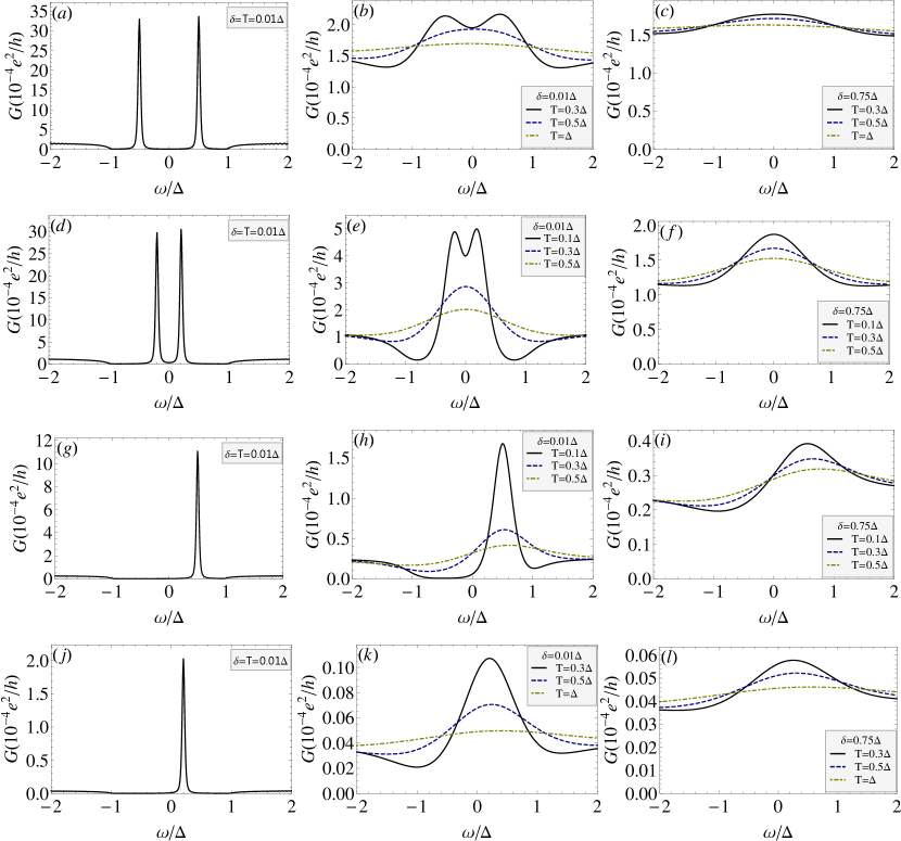
Figure 2: (a-c) The conductance measured by placing the STM tip at a site with a magnetic impurity in an infinite $s$-wave nanowire with $t=2\mu=10\Delta$ and $\gamma=0.001\Delta$. The magnetic impurity induces a YSR state with subgap energy $0.5\Delta$. We show the conductance at high resolution and low temperature [panel (a)], high resolution and high temperature [panel (b)], and low resolution [panel (c)]. (d-f) Similar to Panels (a-c) but with smaller subgap energy $0.2\Delta$. (g-i) Similar to Panels (a-c) but at the site of a nonmagnetic impurity in an infinite $p$-wave nanowire with $t=2\mu=10\Delta$. The impurity induces an Andreev state with energy $0.5\Delta$. (j-l) Similar to Panels (g-i) but with smaller subgap energy $0.2\Delta$.

Fig. 2 shows the differential conductance obtained by tunneling into nontopological subgap states in an infinite nanowire, induced by either magnetic impurities (in the $s$-wave nanowire) or non-magnetic impurities (in the $p$-wave nanowire). At high resolution and low temperature (Fig. 2a,d,g,j) the exact non-zero energy of the subgap state can be extracted from the tunneling spectra. With either high temperatures (Fig. 2b,e,h,k) or low resolutions (Fig. 2c,f,i,l), however, the peaks broaden and could appear to arise from a broadened zero-energy peak. In fact, Fig. 2 shows that with high temperature or low resolution (or both), the tunneling conductance results in the nanowires typically manifest broad features consistent with a zero-energy peak as long as the subgap states are located at $|E|\lesssim 0.5\Delta$. Thus, the observation of broad zero-bias conductance features should not be associated as evidence for the existence of precisely zero-energy MFs since this is also consistent with fermionic subgap states such as ordinary YSR or Andreev bound states. Indeed, the possibility that the experiment of Ref. Nadj-Perge2014Observation is actually observing a YSR state feature instead of a MF state has recently been suggested in the literature Sau2015Bound .

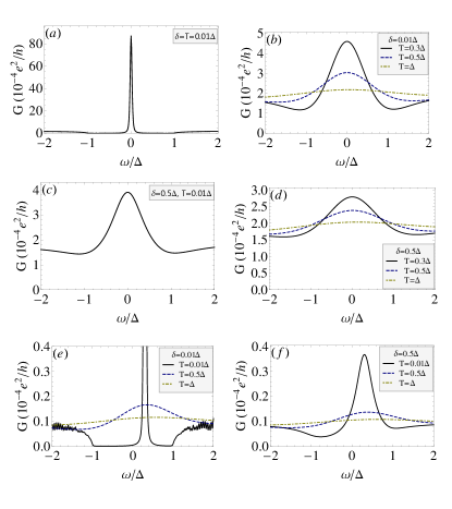
Figure 3: The differential conductance for an STM tunneling measurement on a $p$-wave nanowire with $t=2\mu=10\Delta$ and $\gamma=0.001\Delta$. In panels (a)-(d), the STM tip is placed at the end of the wire, where a zero-energy Majorana mode is found. The results are computed under the conditions of: (a) high resolution and low temperature, (b) high resolution and high temperature, (c) low resolution and high temperature, and (d) low resolution and high temperature. In panels (e)-(f), the STM tip is placed at a site with an impurity, which induces a subgap state with energy $0.3\Delta$, and the results shown correspond to (e) high resolution and (f) low resolution, respectively. The high-temperature results in (b,d,f) are very similar, indicating the difficulty in distinguishing between states at zero energy and states at non-zero but small energy in such circumstances; on the other hand, low-temperature conductance curves with Majoranas in (a,c) can be clearly distinguished from the curves in (e).

We show in Fig. 3(a)-(d) the conductance of a genuine Majorana mode at the end of a clean $p$-wave nanowire, with no other subgap states being present in the system. For comparison, in Fig. 3(e)-(f) we show the conductance of a subgap non-MF state induced by a non-magnetic impurity in an otherwise uniform $p$-wave nanowire. We observe that for low resolutions or high temperatures, the conductance spectra for zero-energy Majorana modes cannot be effectively distinguished from those for non-MF subgap modes. In particular, the high temperature (and/or poor energy resolution) plots in Figs. 3(e) and (f) are indistinguishable from the corresponding plots in Figs. 3(b)-(d), thus confirming that high-temperature STM experiments, as carried out in Ref. Nadj-Perge2014Observation , cannot really confirm the existence of Majorana modes. Thus, only future experiments at lower temperatures and employing better instrumental resolution would be able to conclusively determine the existence or not of MFs in the hybrid Fe nanowire-Pb superconductor system recently studied in Ref. Nadj-Perge2014Observation .

Our work (as well as that presented in Ref. Dumitrescu2014Majorana ) shows that any subgap states, whether MF or not (and whether precisely at zero-energy or not), would manifest very similar STM conductance spectra at high experimental temperatures, and thus the observation of broad, weak, and spectrally diffuse zero bias conductance “peak” cannot be taken as being synonymous with the existence of MFs in the system, as has been done rather uncritically in Ref. Nadj-Perge2014Observation .

V Conclusion

In summary, we have established that the nanowire on superconductor hybrid systems can potentially have very short Majorana localization length even when the induced topological superconducting gap is very small in the nanowire by virtue of the substrate induced strong renormalization of the effective nanowire parameters (e.g. the Fermi velocity, the gap, etc.) because of strong frequency dependence of the relevant self-energy function determining the proximity-induced pair potential in the nanowire. We have shown that this renormalization goes as $R^{-3}$ where $R$ is the effective nanowire confinement size in the transverse direction determining how one-dimensional the system really is (with R going to zero limit being the true 1D nanowire limit). This provides an explanation for why the Majorana localization length could be very small (large) in metallic (semiconducting) nanowires on superconductors since $R\sim 0.5(20)\,{\rm nm}$ in the two systems leads to a large difference in the renormalization effect induced by the substrate. The substrate-induced suppression of the Majorana localization length may have implications for recent efforts Nadj-Perge2014Observation to observe localized Majorana modes in fairly short ($\lesssim 50$nm) ferromagnetic Fe chains on superconducting Pb substrates using STM spectroscopy, providing a possible explanation Peng2014Strong for how the Majorana mode may be spatially highly localized on a sub-nm length scale near the ends of the Fe adatom chain in spite of a very small induced superconducting gap.

But, the definitive observation of spatially localized Majorana fermions (rather than just spatially localized ordinary fermionic subgap states) requires precise energy localization (exactly at mid-gap or zero energy) in addition to strong spatial localization. Such an “energy localization” necessitates an experimental temperature much smaller than the topological superconducting gap. This condition of “energy localization” is absent in the experiment of Ref. Nadj-Perge2014Observation since the temperature is larger than the estimated induced superconducting gap. Thus, the spectral weight of the observed “zero bias” conductance feature is spectrally spread over the whole induced gap, making it difficult to conclude about possible existence of Majorana fermions in spite of the observed spatial localization. In addition, we have shown through explicit numerical simulations that high-temperature and low-resolution tunneling conductance measurements cannot distinguish between Majorana modes and ordinary fermionic subgap states as both manifest broad and weak zero-bias conductance features. The distinction between these two situations necessitates experiments at temperatures (and resolutions) well below the induced superconducting gap energy in the nanowire. We mention in this context that the state of the arts STM experiments on superconductors are routinely carried out at temperatures of $100\,{\rm mK}$ or below Firmo2013Evidence ; *Allan2013Imaging; *ZhouNatPhys2013; HessPRL1990 , and future experiments with much lower temperatures (and much better resolutions) than used in Ref. Nadj-Perge2014Observation can settle the question of whether Majorana fermions have indeed been observed or not in ferromagnetic chains on superconducting substrates. The minimal existence proof of Majorana fermions necessitates the demonstration of both spatial (at wire-ends) and spectral (at zero-energy) localization of the observed excitation.

Lowering temperature (and/or enhancing the topological gap) as well as improving instrumental resolution should lead to the MF-induced ZBCP becoming sharper and stronger [as in Fig. 3(a)-(d)] in longer ferromagnetic chains whereas in shorter chains, the ZBCP should split because of the hybridization between the two Majorana end modes Cheng2009Splitting ; Cheng2010Stable ; DasSarma2012Splitting . (The currently observed zero bias peak in the ferromagnetic chains Nadj-Perge2014Observation is only a very weak fraction ($10^{-4}$) of the quantized value of $2e^{2}/h$ predicted for the Majorana zero modes, and lowering of temperature should enhance its strength Sengupta2001Midgap .) On the other hand, if the observed sub-gap STM conductance features are arising from impurity-induced non-MF subgap bound states [as in Fig. 2 or Fig. 3(e)-(f)], then lowering temperature (and/or increasing the topological gap) and enhancing resolution should clearly show that these accidental subgap states are non-topological and therefore the resultant subgap conductance features are not spectrally located exactly at zero energy. There should not be any energy splitting of such non-MF subgap peaks in shorter chains, also distinguishing them from possible MF peaks. Current experiments Nadj-Perge2014Observation do not actually find any clear evidence for a topological gap in the ferromagnetic chain with the background subgap conductance being typically more than 50% of the normal state conductance, and any definitive claim for the observation of Majorana fermions must necessarily be coupled with the observation of a reasonably well-defined topological gap with background subgap conductance being suppressed by at least one or two orders of magnitude from its current value. In this context, it may be useful to remember that any fermionic subgap bound state in the adatom (Fe)-superconductor (Pb) system will most likely also be localized near the ends of the Fe chain since this is where the impurity potential is the strongest, as was explicitly shown recently Hui2015Majorana for possible YSR states in this system. Indeed a direct numerical diagonalization using model band structures of the Fe/Pb experimental system produces a very large complex of states in the superconducting gap Ji2008High-Resolution , most of which have nothing topological about them (but all of which are likely to contribute to the subgap tunneling conductance), and the complexity of the system therefore makes any straightforward interpretation of the STM data very difficult.

Appendix A Derivation of Effective Hamiltonian

The various terms in the expression of the self-energy [Eq. (15)] are

$$Z = 1-\int\frac{d^{3}k}{\left(2\pi\right)^{3}}\frac{1}{\omega^{2}-\xi_{\bm{k}}^{2}-\Delta_{SC}^{2}}M_{1},$$ (43)

$$Zt_{\bm{r},\bm{r}^{\prime}} = \int\frac{d^{3}k}{\left(2\pi\right)^{3}}e^{i\bm{k}\cdot\left(\bm{r}-\bm{r}^{\prime}\right)}\frac{\xi_{\bm{k}}}{\omega^{2}-\xi_{\bm{k}}^{2}-\Delta_{SC}^{2}}M_{1},$$ (44)

$$Z\bm{\lambda}_{\bm{r},\bm{r}^{\prime}}\cdot\hat{\bm{\sigma}} = \int\frac{d^{3}k}{\left(2\pi\right)^{3}}e^{i\bm{k}\cdot\left(\bm{r}-\bm{r}^{\prime}\right)}\frac{\xi_{\bm{k}}}{\omega^{2}-\xi_{\bm{k}}^{2}-\Delta_{SC}^{2}}M_{2},$$ (45)

$$Z\Delta_{\bm{r},\bm{r}^{\prime}} = -\int\frac{d^{3}k}{\left(2\pi\right)^{3}}e^{i\bm{k}\cdot\left(\bm{r}-\bm{r}^{\prime}\right)}\frac{\Delta_{SC}}{\omega^{2}-\xi_{\bm{k}}^{2}-\Delta_{SC}^{2}}M_{1},$$ (46)

$$Z\bm{\Delta}_{\bm{r},\bm{r}^{\prime}}\cdot\hat{\bm{\sigma}} = -\int\frac{d^{3}k}{\left(2\pi\right)^{3}}e^{i\bm{k}\cdot\left(\bm{r}-\bm{r}^{\prime}\right)}\frac{\Delta_{SC}}{\omega^{2}-\xi_{\bm{k}}^{2}-\Delta_{SC}^{2}}M_{2},$$ (47)

where $M_{1}\equiv t_{s}^{2}B_{s}^{T}B_{s}^{*}+t_{p}^{2}B_{p}^{T}B_{p}^{*}$ and $M_{2}\equiv t_{s}^{2}B_{s}^{T}B_{p}^{*}+t_{p}^{2}B_{p}^{T}B_{s}^{*}$. If we take the specified form of $B_{s}$ and $B_{p}$ [Eq. (19)], they become

$$M_{1}\left(\bm{k}\right) = t_{s}^{2}\cos^{2}\theta+t_{p}^{2}\sin^{2}\theta$$ (48a)

$$M_{2}\left(\bm{k}\right) = t_{s}t_{p}\sin 2\theta\hat{\bm{\sigma}}\cdot\bm{e}_{\bm{k}}$$ (48b)

Further, restricting $\bm{r}$ only at the lattice positions of the nanowire lying on the $x$-axis, we can evaluate the terms exactly as

$$Z = 1-\int\frac{d^{3}k}{\left(2\pi\right)^{3}}\frac{1}{\omega^{2}-\xi_{\bm{k}}^{2}-\Delta_{SC}^{2}}M_{1}\left(\bm{k}\right)$$ (49a)

$$= 1+\frac{\pi\nu}{\sqrt{\Delta_{SC}^{2}-\omega^{2}}}\left(t_{s}^{2}\cos^{2}\theta+t_{p}^{2}\sin^{2}\theta\right)$$

$$Zt_{n>0} = \int\frac{d^{3}k}{\left(2\pi\right)^{3}}e^{ik_{x}na_{{\rm lat}}}\frac{\xi_{\bm{k}}}{\omega^{2}-\xi_{\bm{k}}^{2}-\Delta_{SC}^{2}}M_{1}\left(\bm{k}\right)$$ (49b)

$$= -\pi\nu\frac{\cos nk_{F}a_{{\rm lat}}}{nk_{F}a_{{\rm lat}}}\left(t_{s}^{2}\cos^{2}\theta+t_{p}^{2}\sin^{2}\theta\right)e^{-\frac{n\sqrt{\Delta_{SC}^{2}-\omega^{2}}a_{{\rm lat}}}{v_{F}}}$$

$$Z\bm{\lambda}_{n>0}\cdot\hat{\bm{\sigma}} = \int\frac{d^{3}k}{\left(2\pi\right)^{3}}e^{ik_{x}na_{{\rm lat}}}\frac{\xi_{\bm{k}}}{\omega^{2}-\xi_{\bm{k}}^{2}-\Delta_{SC}^{2}}M_{2}\left(\bm{k}\right)$$ (49c)

$$= -i\pi\nu t_{s}t_{p}\sin 2\theta\hat{\sigma}_{y}\frac{\cos nk_{F}a_{{\rm lat}}+nk_{F}a_{{\rm lat}}\sin nk_{F}a_{{\rm lat}}}{n^{2}k_{F}^{2}a_{{\rm lat}}^{2}}e^{-\frac{n\sqrt{\Delta_{SC}^{2}-\omega^{2}}a_{{\rm lat}}}{v_{F}}}$$

$$Z\Delta_{n} = -\int\frac{d^{3}k}{\left(2\pi\right)^{3}}e^{ik_{x}na_{{\rm lat}}}\frac{\Delta_{SC}}{\omega^{2}-\xi_{\bm{k}}^{2}-\Delta_{SC}^{2}}M_{1}\left(\bm{k}\right)$$ (49d)

$$= \pi\nu\frac{\Delta_{SC}}{\sqrt{\Delta_{SC}^{2}-\omega^{2}}}\frac{\sin nk_{F}a_{{\rm lat}}}{nk_{F}a_{{\rm lat}}}\left(t_{s}^{2}\cos^{2}\theta+t_{p}^{2}\sin^{2}\theta\right)e^{-\frac{n\sqrt{\Delta_{SC}^{2}-\omega^{2}}a_{{\rm lat}}}{v_{F}}}$$

$$Z\bm{\Delta}_{n>0}^{(t)}\cdot\hat{\bm{\sigma}} = -\int\frac{d^{3}k}{\left(2\pi\right)^{3}}e^{ik_{x}na_{{\rm lat}}}\frac{\Delta_{SC}}{\omega^{2}-\xi_{\bm{k}}^{2}-\Delta_{SC}^{2}}M_{2}\left(\bm{k}\right)$$ (49e)

$$= i\pi\nu t_{s}t_{p}\sin 2\theta\hat{\sigma}_{y}\left(\frac{\Delta_{SC}}{\sqrt{\Delta_{SC}^{2}-\omega^{2}}}\frac{\sin nk_{F}a_{{\rm lat}}-nk_{F}a_{{\rm lat}}\cos nk_{F}a_{{\rm lat}}}{n^{2}k_{F}^{2}a_{{\rm lat}}^{2}}\right)e^{-\frac{n\sqrt{\Delta_{SC}^{2}-\omega^{2}}a_{{\rm lat}}}{v_{F}}}$$

The full effective BdG Hamiltonian of the nanowire is then given by substituting these expressions to Eq. (18).

Appendix B Hamiltonian in the strong spin polarization limit

To obtain the Hamiltonian in the limit of strong spin polarization, we start by writing Eq. (18) in momentum space

$$H_{{\rm eff}} = \sum_{k}\left[(\epsilon_{k}-\mu)a_{k}^{\dagger}a_{k}+\lambda_{k}a_{k}^{\dagger}\sigma_{y}a_{k}+\tilde{B}a_{k}^{\dagger}\sigma_{z}a_{k}\right.$$

$$\left.+\Delta_{k}^{\left(t\right)}\left(a_{k\uparrow}a_{-k\uparrow}+a_{k\downarrow}a_{-k\downarrow}+{\rm h.c.}\right)\right.$$

$$\left.+\Delta_{k}\left(a_{k\uparrow}a_{-k\downarrow}+{\rm h.c.}\right)\right],$$

where $a_{k}^{\dagger}=\left(a_{k\uparrow}^{\dagger},a_{k\downarrow}^{\dagger}\right)$, $\epsilon_{k}$ is the Fourier transform of the hopping terms in Eq. (18), $\tilde{B}=Z^{-1}B$ is the renormalized exchange field, while $\lambda_{k}$, $\Delta_{k}$, and $\Delta^{(t)}_{k}$ are the proximity-induced spin-orbit coupling, singlet pairing potential, and triplet pairing potential, respectively. Diagonlizing the first three terms in Eq. (B) gives us the “normal state” dispersion $\xi_{\pm}\left(k\right)=\epsilon_{k}-\mu\pm\sqrt{\tilde{B}^{2}+\tilde{\lambda}_{k}^{2}}$ with eigenvectors

$$\phi_{\pm}\left(k\right)=\frac{1}{2}\left(1\pm\frac{\tilde{B}-i\lambda_{k}}{\sqrt{\tilde{B}^{2}+\lambda_{k}^{2}}},1\mp\frac{\tilde{B}-i\lambda_{k}}{\sqrt{\tilde{B}^{2}+\lambda_{k}^{2}}}\right)^{T}\,.$$ (51)

Following the standard approach Lutchyn2010Majorana ; Alicea2010Majorana , we rewrite the Hamiltonian in this basis with the transformation

$$a_{k}=\phi_{+}\left(k\right)c_{+}\left(k\right)+\phi_{-}\left(k\right)c_{-}\left(k\right),$$ (52)

where $c_{\pm}$ annihilates states in the corresponding normal state bands. Eq. (B) then becomes

$$H_{{\rm eff}} = \sum_{k}\left\{\xi_{+}\left(k\right)c_{+}^{\dagger}\left(k\right)c_{+}\left(k\right)+\xi_{-}\left(k\right)c_{-}^{\dagger}\left(k\right)c_{-}\left(k\right)+\Delta_{k}^{\left(t\right)}\left[c_{+}\left(k\right)c_{+}\left(-k\right)+c_{-}\left(k\right)c_{-}\left(-k\right)+{\rm h.c.}\right]\right.$$ (53)

$$\left.-\frac{i\lambda_{k}\Delta_{k}}{\sqrt{\tilde{B}^{2}+\lambda_{k}^{2}}}\left[c_{+}\left(k\right)c_{+}\left(-k\right)-c_{-}\left(k\right)c_{-}\left(-k\right)+{\rm h.c.}\right]+\frac{\tilde{B}\Delta_{k}}{\sqrt{\tilde{B}^{2}+\lambda_{k}^{2}}}\left[c_{+}\left(k\right)c_{-}\left(-k\right)+{\rm h.c.}\right]\right\}.$$

The pairing terms on the first line correspond to the proximity-induced triplet gap. On the second line, we have additional triplet pairing terms induced from the interplay of the proximity-induced spin-orbit coupling $\lambda_{k}$ and singlet gap $\Delta_{k}$. In the strongly spin-polarized limit where $\tilde{B}\gg\left|\lambda_{k}\right|$, $|\Delta_{k}|$, however, these terms are negligible. The singlet pairing term, also on the second line, is not suppressed at the Hamiltonian level. However, in the strongly spin polarized limit the band basis approximately coincides with the spin basis, and so the singlet pairing potential does not open a gap due to the huge momenta mismatch between the two bands, and may thus be ignored in the effective Hamiltonian.

References

- (1) E. Majorana, Nuovo Cimento 5, 171 (1937)
- (2) N. Read and D. Green, Phys. Rev. B 61, 10267 (2000)
- (3) A. Y. Kitaev, Phys. Usp. 44, 131 (2001)
- (4) L. Fu and C. L. Kane, Phys. Rev. Lett. 100, 096407 (2008)
- (5) J. D. Sau, R. M. Lutchyn, S. Tewari, and S. Das Sarma, Phys. Rev. Lett. 104, 040502 (2010)
- (6) C. Nayak, S. H. Simon, A. Stern, M. Freedman, and S. Das Sarma, Rev. Mod. Phys. 80, 1083 (2008)
- (7) S. Das Sarma, M. Freedman, and C. Nayak, “Majorana zero modes and topological quantum computation,” (2015), arXiv:1501.02813
- (8) J. D. Sau, S. Tewari, R. M. Lutchyn, T. D. Stanescu, and S. Das Sarma, Phys. Rev. B 82, 214509 (2010)
- (9) R. M. Lutchyn, J. D. Sau, and S. Das Sarma, Phys. Rev. Lett. 105, 077001 (2010)
- (10) Y. Oreg, G. Refael, and F. von Oppen, Phys. Rev. Lett. 105, 177002 (2010)
- (11) S. B. Chung, H.-J. Zhang, X.-L. Qi, and S.-C. Zhang, Phys. Rev. B 84, 060510 (2011)
- (12) M. Duckheim and P. W. Brouwer, Phys. Rev. B 83, 054513 (2011)
- (13) T.-P. Choy, J. M. Edge, A. R. Akhmerov, and C. W. J. Beenakker, Phys. Rev. B 84, 195442 (2011)
- (14) S. Nadj-Perge, I. K. Drozdov, B. A. Bernevig, and A. Yazdani, Phys. Rev. B 88, 020407 (2013)
- (15) V. Mourik, K. Zuo, S. M. Frolov, S. R. Plissard, E. P. A. M. Bakkers, and L. P. Kouwenhoven, Science 336, 1003 (2012)
- (16) M. T. Deng, C. L. Yu, G. Y. Huang, M. Larsson, P. Caroff, and H. Q. Xu, Nano Lett. 12, 6414 (2012)
- (17) L. P. Rokhinson, X. Liu, and J. K. Furdyna, Nat. Phys. 8, 795 (2012)
- (18) A. Das, Y. Ronen, Y. Most, Y. Oreg, M. Heiblum, and H. Shtrikman, Nat. Phys. 8, 887 (2012)
- (19) H. O. H. Churchill, V. Fatemi, K. Grove-Rasmussen, M. T. Deng, P. Caroff, H. Q. Xu, and C. M. Marcus, Phys. Rev. B 87, 241401 (2013)
- (20) A. D. K. Finck, D. J. Van Harlingen, P. K. Mohseni, K. Jung, and X. Li, Phys. Rev. Lett. 110, 126406 (2013)
- (21) S. Nadj-Perge, I. K. Drozdov, J. Li, H. Chen, S. Jeon, J. Seo, A. H. MacDonald, B. A. Bernevig, and A. Yazdani, Science 346, 602 (2014)
- (22) D. Bagrets and A. Altland, Phys. Rev. Lett. 109, 227005 (2012)
- (23) D. I. Pikulin, J. P. Dahlhaus, M. Wimmer, H. Schomerus, and C. W. J. Beenakker, New Journal of Physics 14, 125011 (2012)
- (24) X. Liu, J. D. Sau, and S. D. Sarma, “Universal spin-triplet superconducting correlations of majorana fermions,” (2015), arXiv:1501.07273
- (25) M. Cheng, R. M. Lutchyn, V. Galitski, and S. Das Sarma, Phys. Rev. Lett. 103, 107001 (2009)
- (26) M. Cheng, K. Sun, V. Galitski, and S. Das Sarma, Phys. Rev. B 81, 024504 (2010)
- (27) S. Das Sarma, J. D. Sau, and T. D. Stanescu, Phys. Rev. B 86, 220506 (2012)
- (28) J. D. Sau, R. M. Lutchyn, S. Tewari, and S. Das Sarma, Phys. Rev. B 82, 094522 (2010)
- (29) T. D. Stanescu, J. D. Sau, R. M. Lutchyn, and S. Das Sarma, Phys. Rev. B 81, 241310 (2010)
- (30) Y. Peng, F. Pientka, L. I. Glazman, and F. von Oppen, Phys. Rev. Lett. 114, 106801 (2015)
- (31) H.-Y. Hui, P. M. R. Brydon, J. D. Sau, S. Tewari, and S. D. Sarma, Sci. Rep. 5, 8880 (2015)
- (32) E. Dumitrescu, B. Roberts, S. Tewari, J. D. Sau, and S. D. Sarma, Phys. Rev. B 91, 094505 (2015)
- (33) J. Li, H. Chen, I. K. Drozdov, A. Yazdani, B. A. Bernevig, and A. H. MacDonald, Phys. Rev. B 90, 235433 (2014)
- (34) A. Heimes, D. Mendler, and P. Kotetes, New Journal of Physics 17, 023051 (2015)
- (35) S. Takei and V. Galitski, Phys. Rev. B 86, 054521 (2012)
- (36) J. Wang, M. Singh, M. Tian, N. Kumar, B. Liu, C. Shi, J. K. Jain, N. Samarth, T. E. Mallouk, and M. H. W. Chan, Nat. Phys. 6, 389 (2010)
- (37) A. Yazdani, B. A. Jones, C. P. Lutz, M. F. Crommie, and D. M. Eigler, Science 275, 1767 (1997)
- (38) S.-H. Ji, T. Zhang, Y.-S. Fu, X. Chen, X.-C. Ma, J. Li, W.-H. Duan, J.-F. Jia, and Q.-K. Xue, Phys. Rev. Lett. 100, 226801 (2008)
- (39) F. Pientka, L. I. Glazman, and F. von Oppen, Phys. Rev. B 88, 155420 (2013)
- (40) Y. Kim, M. Cheng, B. Bauer, R. M. Lutchyn, and S. Das Sarma, Phys. Rev. B 90, 060401 (2014)
- (41) P. M. R. Brydon, S. Das Sarma, H.-Y. Hui, and J. D. Sau, Phys. Rev. B 91, 064505 (2015)
- (42) J. D. Sau and S. D. Sarma, Nat. Commun. 3, 964 (2012)
- (43) I. A. Firmo, S. Lederer, C. Lupien, A. P. Mackenzie, J. C. Davis, and S. A. Kivelson, Phys. Rev. B 88, 134521 (2013)
- (44) M. P. Allan, F. Massee, D. K. Morr, J. Van Dyke, A. W. Rost, A. P. Mackenzie, C. Petrovic, and J. C. Davis, Nat. Phys. 9, 468 (2013)
- (45) B. B. Zhou, S. Misra, E. H. da Silva Neto, P. Aynajian, R. E. Baumbach, J. D. Thompson, E. D. Bauer, and A. Yazdani, Nat. Phys. 9, 474 (2013)
- (46) H. F. Hess, R. B. Robinson, and J. V. Waszczak, Phys. Rev. Lett. 64, 2711 (1990)
- (47) J. D. Sau and P. M. R. Brydon, “Bound states of a ferromagnetic wire in a superconductor,” (2015), arXiv:1501.03149
- (48) T. Kontos, M. Aprili, J. Lesueur, and X. Grison, Phys. Rev. Lett. 86, 304 (2001)
- (49) A. L. Fauchère, W. Belzig, and G. Blatter, Phys. Rev. Lett. 82, 3336 (1999)
- (50) K. Sengupta, I. Zutic, H.-J. Kwon, V. M. Yakovenko, and S. Das Sarma, Phys. Rev. B 63, 144531 (2001)
- (51) R. M. Lutchyn, T. D. Stanescu, and S. Das Sarma, Phys. Rev. Lett. 106, 127001 (2011)
- (52) L. Yu, Acta Phys. Sin. 21, 75 (1965)
- (53) H. Shiba, Prog. Theor. Phys. 40, 435 (1968)
- (54) A. I. Rusinov, Eksp. Teor. Fiz. Pisma. Red. 9, 146 (1968), [JETP Lett. 9, 85 (1969)]
- (55) A. A. Zyuzin, D. Rainis, J. Klinovaja, and D. Loss, Phys. Rev. Lett. 111, 056802 (2013)
- (56) A. M. Lobos and S. D. Sarma, New J. Phys. 17, 065010 (2015)
- (57) J. Alicea, Phys. Rev. B 81, 125318 (2010)