Evaluation of spatial audio reproduction schemes for application in hearing aid research

Abstract

Loudspeaker-based spatial audio reproduction schemes are increasingly used for evaluating hearing aids in complex acoustic conditions. To further establish the feasibility of this approach, this study investigated the interaction between spatial resolution of different reproduction methods and technical and perceptual hearing aid performance measures using computer simulations. Three spatial audio reproduction methods – discrete speakers, vector base amplitude panning and higher order ambisonics – were compared in regular circular loudspeaker arrays with 4 to 72 channels. The influence of reproduction method and array size on performance measures of representative multi-microphone hearing aid algorithm classes with spatially distributed microphones and a representative single channel noise-reduction algorithm was analyzed. Algorithm classes differed in their way of analyzing and exploiting spatial properties of the sound field, requiring different accuracy of sound field reproduction. Performance measures included beam pattern analysis, signal-to-noise ratio analysis, perceptual localization prediction, and quality modeling. The results show performance differences and interaction effects between reproduction method and algorithm class that may be used for guidance when selecting the appropriate method and number of speakers for specific tasks in hearing aid research.

1 Introduction

Hearing aids are evolving from simple amplifiers to complex systems that are aware of the spatial configuration and contents of their acoustic surroundings (Kates, 2008). Moreover, the interaction between hearing aids and users is gaining increasing attention (Tessendorf et al., 2011). This development causes an increase in the complexity of hearing aids and their use which in turn requires improved evaluation methods in order to demonstrate the properties and benefits of the systems. One way of achieving this is to perform evaluations in real acoustic environments; however, this approach is costly and does not provide completely controllable and reproducible experimental conditions. Laboratory studies, on the other hand, are efficient and reproducible but performance of hearing aid algorithms in real environments and under laboratory conditions often differs substantially due to a different subject behavior (e.g., Smeds et al., 2006) or as a consequence of oversimplification of the acoustic scenarios (Cord et al., 2004; Bentler, 2005). This motivates the reproduction of complex acoustic environments in the laboratory using loudspeaker-based spatial audio reproduction methods to provide controllable and reproducible realistic experimental conditions for hearing aid evaluations. Available reproduction methods, however, have not yet been evaluated systematically in combination with multi-microphone hearing aid algorithms.

Typical applications of spatial audio reproduction systems are sound reinforcement for theaters and cinemas (Brandenburg et al., 2004), music reproduction (Nettingsmeier, 2010), audio reproduction for computer games (Olaiz et al., 2009), room auralization (Favrot and Buchholz, 2009, 2010), and applications in hearing research (Seeber et al., 2010). Each application has its own requirements regarding listening area, tolerance to spatial or timbral artifacts, maximum technical complexity, computational complexity, and latency. In contrast to music- and media-reproduction systems, constraints regarding the size of the listening area are comparably loose in research applications, since typically only a single listener or a small group of listeners is addressed simultaneously. The system layout in theater and cinema applications often uses an asymmetric distribution of loudspeakers, e.g., 5.1 (ITU-R, 2012) or 22.2 (Hamasaki et al., 2005; Hamasaki, 2011), to achieve a higher spatial resolution in the frontal hemisphere. Applications in hearing research commonly use horizontal circular layouts with a regular loudspeaker distribution. Methods for generation of the loudspeaker signals include vector base amplitude panning (VBAP; Pulkki, 1997), higher order ambisonics (HOA; Daniel, 2001) and wave field synthesis (WFS; Berkhout et al., 1993; Spors et al., 2008). Common to all loudspeaker-based spatial audio reproduction methods is their limited spatial resolution due to the finite number of speakers involved in the reproduction. The type, number and spatial distribution of artifacts related to this limitation differ substantially between methods.

Theoretical and perceptual limitations of loudspeaker-based spatial audio reproduction schemes have been studied extensively (e.g., Landone and Sandler, 1999; Daniel et al., 2003; Ahrens and Spors, 2008). Many studies focus primarily on music reproduction (e.g., Bates et al., 2007; Guastavino and Katz, 2004). Other studies measure interaural time difference (ITD) and interaural level difference (ILD) as a predictor of perceptual localization performance (Daniel, 2001; Carlsson, 2004; Pulkki and Hirvonen, 2005; Benjamin et al., 2010; Bertet et al., 2013). These studies thoroughly investigated the perceptual properties of the reproduction methods. Although the physical sound field is not correctly reproduced, it was shown that the perceptual impression can be rendered almost perfectly by exploiting properties of the human (binaural) hearing system. However, when the reproduced sound is processed by a hearing aid algorithm with spatially distributed microphones prior to presenting it to the subject, both physical characteristics of the reproduced sound field and perceptual aspects play a role in assessing the reproduction quality. If the sound field sampled by the spatially distributed microphones physically deviates from the original sound field, the function of the algorithm might be hampered, possibly leading to a decreased algorithm performance and perceptually audible artifacts. To assess this possibly detrimental effect, knowledge of the details of multi-microphone processing in hearing aids is required.

Hamacher et al. (2005) provide an overview of state-of-the-art algorithms applied in hearing aids. They distinguish between five classes of algorithms: Directional microphones, single channel noise reduction, multi-band dynamic compression, feedback suppression, and classification. In their first class they list all algorithms that use spatially distributed microphones. These include first-order and higher-order microphone arrays (e.g., Widrow and Luo, 2003; Rohdenburg et al., 2007), extended adaptive algorithms (e.g., Elko and Pong, 1995; Spriet et al., 2005), and binaural noise reduction schemes (e.g., Kollmeier et al., 1993; Wittkop et al., 1997; Wittkop and Hohmann, 2003). Whereas the functioning of these algorithms explicitly depends on the spatial properties of the sound field in the small area covered by the microphones, i.e., close to the head of the hearing-aid user, the other classes like single channel noise reduction and dynamic compression, depend only implicitly on the spatial properties of the surrounding, e.g., as a result of head shadowing, and in the sense that they potentially modify spatial cues sensed by the listener. Depending on which spatial aspects of the sound field are exploited by a specific algorithm, its performance may therefore be affected differently by the specific limitations of a reproduction method in reproducing the sound field at the head. Thus, several algorithm classes need to be tested in combination with different reproduction methods to assess the interaction between algorithm class and reproduction method.

Only one simulation study by Oreinos et al. (2013) evaluated performance of two different hearing aid algorithms with spatially distributed microphones, an adaptive differential microphone and an interaural coherence-based directional filter, in a sound field reproduced by a 7th order HOA system. Data show that up to a certain frequency the HOA system has no significant effect on the algorithm performance, and that the effect is larger for the adaptive directional microphone than for the interaural coherence-based directional algorithm. However, while showing the principle feasibility of the approach, only a single reproduction method and a fixed array size were considered.

This simulation study systematically evaluates the interaction of reproduction method, array size and different classes of hearing aid algorithms with spatially distributed microphones. The effect of three spatial audio reproduction methods on the performance of three conceptually different classes of multi-microphone hearing aid algorithms, a static binaural beamformer with three microphones at each ear (Rohdenburg et al., 2007), an adaptive directional microphone with two microphones at one ear (Elko and Pong, 1995) and an interaural coherence-based binaural noise reduction algorithm with one microphone at each ear (Grimm et al., 2009) was assessed. Furthermore, a standard single-channel noise reduction scheme (Ephraim and Malah, 1984) was included in the study. Small to medium-sized loudspeaker arrays with 4 to 72 loudspeakers in a horizontal circular configuration were tested, representing the size range and type of systems commonly used in experimental hearing research. Loudspeaker signals were generated with three different methods, which can be interpreted as three different methods of spatial interpolation: The selection of the nearest speaker (NSP) to a virtual sound source uses only a single loudspeaker at a time. With vector base amplitude panning (VBAP) two loudspeakers are used to interpolate virtual source positions not covered by a loudspeaker. In higher order ambisonics (HOA) all loudspeakers contribute to the spatial image. Unless near-field compensation is applied to HOA, these methods commonly reproduce phantom sources in the distance of the loudspeaker array, i.e., they do not encode the curvature of the wave fronts, and distances can only be coded by loudness, spectral cues caused by air absorption and, in case of closed rooms, by the direct-to-reverberant ratio of sounds. Wave field synthesis (WFS) is able to reproduce the curvature of wave fronts by synthesizing the whole sound field of a virtual source. However, WFS differs in its spatial distribution and type of artifacts, and thus does not directly compare to the other mentioned reproduction methods. Specifically, for a comparable amount of artifacts in a single point for a given frequency bandwidth, WFS requires a much higher number of speakers than VBAP or HOA; thus WFS was not considered here. For an assessment of the effects of reproduction systems, all signals were generated by convolution of the loudspeaker signals with anechoic binaural head-related impulse responses (HRIR) of a head-and-torso simulator (HATS) wearing a pair of behind-the-ear hearing aids. In this study only two-dimensional (2D) sound reproduction was considered. Although this corresponds to commonly used setups used in hearing aid research, it brings several limitations: On the perceptual side, the horizontal plane is considered most important for localization. For plausible reproduction, however, full immersion is needed, which implies 3D reproduction. The technical limitation of 2D sound reproduction is that a vertical distribution of microphones in hearing aids can not be tested. Also, for off-center listening, the spatial distribution of sound intensity differs from the 3D case (Daniel, 2001). Still, in many applications of hearing aid research a 2D reproduction might be sufficient, because the largest interaural differences (ILD and ITD) are produced in the horizontal plane. Additionally, also beamformers mostly operate in this range.

In objective hearing aid algorithm evaluation instrumental performance measures or performance measures based on perceptual models are commonly applied (Eneman et al., 2008). To assess spatial audio reproduction methods, performance measures of the free field condition served as a reference in this study. Differences in performance to the reference condition indicate the lumped effect of the properties of the reproduction method on algorithm performance. The selection of performance measures depends on the choice of algorithms to be tested. Beam patterns (e.g., Luo et al., 2002), i.e., the frequency- and azimuth dependent array gains, were analyzed for the static beamformer. For all algorithms, the signal-to-noise ratio (SNR) improvement as a function of input SNR and frequency was used. Since the processed signals are usually presented to a human listener, the predictions of a perceptual localization model and a monaural perceptual similarity measure were also applied as baseline measures.

The remainder of the paper is organized as follows: Section 2.1 describes the used spatial audio reproduction methods. Algorithm classes are described in section 2.2, section 2.3 defines the set of relevant performance measures and the simulation methods. Results are presented and discussed in section 3 and 4, respectively. Conclusions are given in section 5.

2 Methods

2.1 Spatial audio reproduction methods

In this study a spatial audio reproduction method is defined as a set of driving functions in the form of a set of linear filters ${\bf g}_{\bf r}=[g_{1},\dots,g_{N}]$ which generate loudspeaker signals ${\bf x}(t)=[x_{1}(t),\dots,x_{N}(t)]$ by convolution of the audio signal $x_{r}(t)$ of a single omnidirectional (virtual) sound source at the position ${\bf r}$ in space with the filters ${\bf g}_{\bf r}$:

$${\bf x}(t)={\bf g}_{\bf r}*x_{r}(t)$$ (1)

A reproduction system is an arrangement of $N$ loudspeakers at the positions ${\bf s}_{k},\,k=1\dots N$. Only regular, horizontal, circular reproduction systems with even numbers of loudspeakers are addressed here. Without loss of generality, the center of the reproduction system is assumed to be at the origin of the coordinate system.

Each driving function $g_{k}$ can be split into a scalar weight $w_{k}$ which depends on the position ${\bf r}$ of the source, and a transmission part $h_{k}$ which depends only on the distance $||{\bf r}||$ of the source from the origin. $h_{k}$ is the acoustic model of the source, here consisting of a distance-dependent delay $\tau=||{\bf r}||/c$ and an attenuation,

$$g_{k}({\bf r})=\frac{w_{k}({\bf r})}{||{\bf r}||}\cdot\delta(\tau),$$ (2)

where $\delta(\tau)$ is the dirac-function and $c$ is the speed of sound. The weights $w_{k}({\bf r})$ depend on the specific reproduction method and will be defined below.

2.1.1 Nearest speaker (NSP)

The simplest spatial audio reproduction method selects the loudspeaker $k_{min}$ with the least distance to the source for reproduction. The driving weights are thus

$$w_{k}=\left\{\begin{array}[]{ll}1&k=k_{min}\\ 0&{\textrm{otherwise}}\end{array}\right..$$ (3)

This reproduction method is equivalent to placing loudspeakers at the positions of the sources, which is commonly done in hearing aid evaluation (e.g., Greenberg et al., 2003).

2.1.2 Vector base amplitude panning (VBAP)

Horizontal vector base amplitude panning as defined by Pulkki (1997), uses the closest pair $l,m$ of loudspeakers for reproduction of a source. Driving weights $w_{l}$ and $w_{m}$ are calculated from the unit vector of the source $\hat{{\bf r}}={{\bf r}}\cdot||{\bf r}||^{-1}$ and the unit vectors of the closest loudspeakers, $\hat{{\bf s}}_{l}$ and $\hat{{\bf s}}_{m}$, with the loudspeaker matrix ${\bf S}_{l,m}=\left[\hat{{\bf s}}_{l}\,\hat{{\bf s}}_{m}\right]^{\bf T}$ as

$$\left[w_{l}\,w_{m}\right]=\hat{\bf r}^{\bf T}{\bf S}_{l,m}^{-1},$$ (4)

$w_{k}=0$ for $k\neq l,m$. With only two loudspeakers, this method is equivalent to conventional stereo panning.

2.1.3 Higher order ambisonics (HOA)

Higher order ambisonics (HOA) is based on the expansion of the sound field around a single point using spherical harmonics (3D) or cylindrical harmonics (2D) (Daniel, 2001). With increasing truncation order of the expansion, the size of the area in which the sound field is well approximated is increasing. Here, only horizontal higher order ambisonics without near field compensation is considered. In the case of single virtual sound sources, i.e., opposed to recorded sources in HOA format, and a regular reproduction system, the encoding and decoding can be combined, which drastically reduces complexity (Neukom, 2007):

$$w_{k}=\frac{\sin\left(\frac{1}{2}(N-1)\varphi_{k}\right)}{N\sin\left(\frac{1}{2}\varphi_{k}\right)},$$ (5)

with the azimuth $\varphi_{k}$ between the source and the $k$th loudspeaker, and the total number of loudspeakers $N$. With these driving weights the method corresponds to the ’basic’ HOA method (Daniel, 2001). The minimum number of loudspeakers for a given ambisonics order $m$ is $N_{min}=2m+1$. However, in this study only even numbers of $N$ were used, thus the smallest even number of loudspeakers for a given integer ambisonics order $m$ is $N_{even}=2(m+1)$. Accordingly, for any given number of loudspeakers $N$, the largest integer ambisonics order $m=\frac{N}{2}-1$ for even $N$ was used. Coloration artifacts due to spatial aliasing occur if the number of loudspeakers is larger than the minimal number for a given order (Solvang, 2008). However, this effect is small in the current study, because only one more loudspeaker than the minimally required number of speakers was used. Spatial aliasing occurs if

$$kr>\frac{1}{2}N_{min},$$ (6)

with the wave number $k=\frac{2\pi f}{c}$, the listening position $r$, i.e., the distance from the origin, and the speed of sound $c$. This equation can serve as a predictor of the usable bandwidth for a given number of loudspeakers, e.g., $f\leq\frac{c}{4\pi r}N_{min}$, or as a rough guide for choosing the number of loudspeakers for a given application and frequency range, $N\geq\frac{4\pi r}{c}f$. In the case of prediction of binaural listening, $r$ is approximated by the distance of the ear which is further away from the origin.

2.1.4 Test signal generation

The test signals, i.e., the input signals of the hearing aid processing for the instrumental measures, and the input signals of the perceptual models, were generated by convolution of the loudspeaker signals $x_{k}(t)$ (Eq. 1) with HRIR $h({\bf r},t)$ of a Brüel & Kjær HATS in an anechoic room (Kayser et al., 2009),

$$x({\bf r},t)=\sum\limits_{k=1}^{N}h({\bf s}_{k}-{\bf r},t)*x_{k}(t),$$ (7)

where the star denotes convolution, and ${\bf r}$ is the listener position. The database provides HRIR for the in-ear microphones of the HATS as well as the HRIR of six hearing aid microphones, three on each side. HRIR for a distance $d$ between loudspeaker and the center of the head of 0.8 m and 3 m exist in the database. In this study the HRIRs were used for a distance of 3 m, and zero degree elevation, sampled with a spatial resolution of 5 degrees. For the central listening position no interpolation of the HRIR was required. Off-center listening positions, shifted by 0.1 and 0.5 m to the side, were achieved by applying the distance-dependent gains $g=3/d$ and delays $\tau=d/c$ to the HRIRs, and by independent interpolation of the amplitude and phase in the spectrum of the HRIR. The interpolation method produces amplitude errors below 2 dB and only negligible errors of group delay when comparing an interpolated HRIR from two HRIR separated by 10 degree with the corresponding measured HRIR. In the database the HRIRs are sampled with 5 degrees; thus, the expected interpolation error is likely to be smaller. For the experiments based on the perceptual localization model predictions, the in-ear microphone channels of the HRIR database were used, corresponding to channels 1 and 2 in Kayser et al. (2009). For evaluation of hearing aid algorithms, the appropriate channels for the respective hearing aid algorithm were used. For the binaural beamformer these were all six hearing aid channels, for the ADM the front and rear microphones of the left hearing aid, for the binaural noise reduction the front microphones of the left and right hearing aid, and for the single channel noise reduction the front microphone of the left hearing aid.

2.1.5 Reference signal generation

Reference signals were generated by a convolution of the sound source signal with the interpolated anechoic HRIR corresponding to the source direction and distance, which is equivalent to a free field reproduction of the source signal.

2.2 Hearing aid algorithms

Four representative hearing aid algorithms from different classes were selected for analysis. Three of the algorithms are based on spatially separated microphones, with different spatial sensitivity. The fourth algorithm is a standard single-channel noise reduction scheme. All algorithms were implemented in C++ within a software platform for hearing aid algorithm development (Grimm et al., 2006).

2.2.1 Static binaural beamformer

A binaural multi-microphone beamformer algorithm (Rohdenburg et al., 2007) was selected for the assessment of reproduction methods because this algorithm, with six spatially separated microphones, is particularly sensitive to errors in the microphone signals and the sound field reproduction. From the different versions of the beamformer introduced by Rohdenburg et al. (2007), the fixed minimum variance distortionless response beamformer without a general sidelobe canceler was chosen. A diffuse noise field was assumed, and a sampled propagation vector was used, which was matched with the same HRIR as used in the other parts of this study (Kayser et al., 2009, see section 2.1.4 for details). To preserve binaural cues, a real-valued time-variant post filter was applied. With this post filter, the binaural cues of both the target and the noise signal are preserved. In a condition with a single target and an artificial diffuse noise, an absolute SNR improvement of about 6 to 14 dB can be reached, see Fig. 1.

2.2.2 Adaptive differential microphone (ADM)

The ADM algorithm is based on a front-facing and a back-facing microphone signal (Elko and Pong, 1995) as typically found in behind-the-ear hearing aids. These signals are generated by two delay-and-sum beamformers using a single pair of omnidirectional microphones. A mixing weight is adapted to minimize the back-facing signal in the input signal. This algorithm can achieve signal-to-noise ratio (SNR) improvements of up to 20 dB in anechoic conditions with a single noise source, and approximately 3 to 6 dB in diffuse-noise situations, see Fig. 1.

2.2.3 Binaural noise reduction

The binaural noise reduction scheme estimates the interaural coherence function in multiple frequency bands, to steer a Wiener-like filter (Kollmeier et al., 1993; Wittkop and Hohmann, 2003). In this study an omni-directional variant is used (Grimm et al., 2009; Luts et al., 2010), which estimates the interaural coherence from the interaural phase difference (IPD) fluctuations. In each frequency band and time frame, the IPD is measured and transformed onto the complex plane. The vector strength, i.e., the absolute value of the low-pass filtered complex-valued IPD is taken as a measure of the coherence $\gamma$:

$$\gamma=\left|\left\langle e^{i\,\textrm{IPD}}\right\rangle_{\tau}\right|$$ (8)

The low pass filter $\langle\cdots\rangle_{\tau}$ with the time constant $\tau$ was implemented as a first-order IIR low-pass filter. The applied gain in each frequency band is $G=\gamma^{\beta}$. In this study, the algorithm settings of Luts et al. (2010) were used, i.e., $\tau=40$ ms and a frequency-dependent efficiency coefficient $\beta$ ranging from 0 to 0.5.

With this algorithm SNR improvements of about 4 dB can be achieved in real acoustic environments at frequencies above 1 kHz and at about 0 dB input SNR, see Fig. 1.

2.2.4 Single channel noise reduction

The single channel noise reduction algorithm after Ephraim and Malah (1984) was chosen as a typical representative of the class of single channel algorithms. The original algorithm with an optimal noise spectrum estimator using perfect a-priori knowledge of the noise signal was used. With this “oracle” algorithm an SNR improvement of about 10 dB was achieved at negative SNRs, independent of the frequency, see Fig. 1.

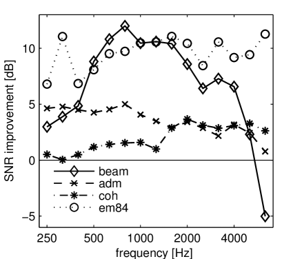
Figure 1: Frequency dependent SNR benefit of the four tested algorithms in a diffuse noise environment (see Sec. 2.3.2), averaged across all tested input SNRs from $-20$ to 20 dB and listening positions, in a free field condition. The SNR benefit is an instrumental measure and not necessarily related to any perceptual benefit.

2.3 Performance measures

This study assesses to what extent commonly applied performance measures are affected by the choice and resolution of the spatial audio reproduction method. Thus, for each reproduction method and number of loudspeakers a full technical evaluation of each of the hearing aid algorithms was performed. The outcome was then compared to a free field condition as a reference (see Sec. 2.1.5). An error function was defined for each performance measure to provide a quantitative analysis of differences compared to the reference.

Suitable measures were applied to each tested algorithm. An analysis of the beam pattern (Sec. 2.3.1) was applied to the static beamformer. The SNR improvement in a simulated diffuse noise condition (Sec. 2.3.2) was applied to all algorithms. Perceptual localization performance was predicted using a perceptual localization model, and monaural audio quality was predicted using a perceptual spectral distance model (Sec. 2.3.3).

2.3.1 Beam pattern analysis

Static beamformers are commonly described by their beam patterns, i.e., the gain $G(\alpha,f)$ as a function of azimuth $\alpha$ and frequency $f$. Here, root-mean-square gain deviation of $\Delta G=20\log_{10}(G_{ref})-20\log_{10}(G_{test})$ averaged across all azimuths $\alpha=0,5,10,\dots,355$ between the reference beam pattern $G_{ref}$ (free field) and a test beam pattern $G_{test}$ (achieved with a specific spatial reproduction method) was taken as a frequency-dependent measure of reproduction method performance. The beam pattern was calculated in third-octave bands. $G_{ref}$ and $G_{test}$ were limited to $-35$ dB for values below $-35$ dB to avoid an excessive effect of Nulls. The error function can be written as:

$$E(f)=\sqrt{\sum_{\alpha}(\Delta G(\alpha,f))^{2}}$$ (9)

The beam patterns were calculated using HRIRs (Kayser et al., 2009) and thus include the effect of the HATS. Exemplary beam patterns and a schematic visualization of the beam error are shown in Figure 2.

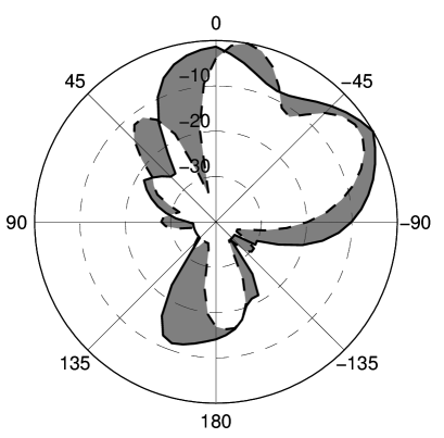
Figure 2: Exemplary beam pattern at 2 kHz in the reference condition, i.e., free field (dashed line) and with 6-channel VBAP (solid line). The RMS of the difference defines the beam pattern error (shaded area).

2.3.2 SNR improvement analysis

Most hearing aid algorithms modify the SNR to some extent – some algorithms like beamformers and noise reduction schemes by intention, others as an artifact. Thus these algorithms are often characterized by the SNR improvement behavior, i.e., the difference of the SNR at the output $R_{o}$ and at the input $R_{i}$ as a function of input SNR.

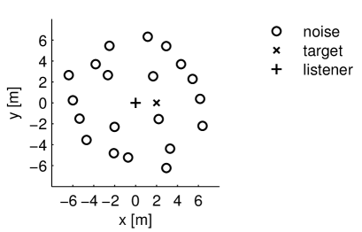
Figure 3: Simulated diffuse noise situation for the SNR evaluation. Circles indicate the positions of noise sources, each radiating a cafeteria-like noise signal. The diagonal cross indicates the position of the frontal target speech signal.

Here, the SNR behavior in a diffuse noise situation with a single target speech signal from the front and 20 spatially distributed cafeteria-noise sources (see Figure 3) was chosen as a measure of reproduction method performance. The target stimulus was a 8.4-second segment of a female monologue. The diffuse noise environment was created by adding cafeteria-noise sound sources from different directions and with an attenuation corresponding to the respective distances. Each of the sources was simulated using the method described in 2.1.4. Early reflections and diffuse reverberation were not added. The noise stimuli were non-overlapping segments taken from a single-channel recording in a real cafeteria, containing a clutter of cutlery noises, babble and moved chairs. The long-term SNR improvement of the hearing aid algorithm $\Delta R(f)$ was estimated in third-octave bands, for nine different nominal broad-band input SNRs $R_{i,n}=-20,-15,-10,\dots,20$ dB. As error measure the root-mean-square difference between reference condition with free field and the test condition with application of the spatial audio reproduction method was computed:

$$E(f)=\sqrt{\frac{1}{9}\sum_{R_{i,n}}\left(\Delta R_{ref}(f)-\Delta R_{test}(f)\right)^{2}}$$ (10)

An exemplary SNR improvement of the binaural noise reduction algorithm is shown in Figure 4.

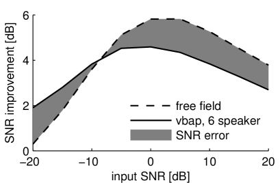
Figure 4: Exemplary SNR improvement of binaural noise reduction in the reference condition, i.e., free field (dashed line) and with 6-channel VBAP (solid line). The RMS of the difference averaged across all input SNRs defines the SNR improvement error (shaded area).

2.3.3 Analysis of errors in perceptual measures of localization and spectral distortion

For modeling source localization, the binaural model of Dietz et al. (2011) was used. It estimates the interaural time difference (ITD) and the interaural level difference (ILD) in auditory frequency bands. An interaural coherence function $\gamma$ is calculated to select only those “glimpses”, i.e., time-frequency signal components, with a high interaural coherence ($\gamma>0.98$) and a rising coherence slope. Only these time-frequency components are assumed to contain reliable perceptual binaural cues. In those frequency bands where temporal fine-structure is available to human listeners (12 bands with center frequencies from 236 to 1296 Hz), the fine-structure ITD is used, and ambiguities are resolved by means of the sign of the ILD, i.e., ILD is only used for disambiguation and not explicitly for estimation of source direction. Direction of arrival (DOA) estimates are interpolated from a look-up table, derived from anechoic HRIRs of the HATS. In this model version, envelope ITDs are used in frequency bands from 1296 Hz to 4 kHz to gather a second DOA estimate. Since only single sources were taken into account in this study, the estimated direction of arrival $\alpha$ was averaged across all selected glimpses of the test stimulus, for fine-structure frequency bands and envelope frequency bands separately.

Based on the localization model output, the perceptual localization error (PLE) was defined as the RMS difference between the estimated direction of arrival in a free field, $\alpha_{ref}$, and the estimated direction of arrival measured with the tested reproduction method, $\alpha_{test}$, for all nominal target directions from $-75$ to 75 degrees in steps of 5 degrees. This limited azimuth range was chosen to avoid problems of the model at lateral signal sources. A small PLE indicates that the predicted perceptual localization does not depend on the reproduction method, whereas for high PLE values the reproduction method has an effect on the predicted perceptual localization. Comparison with the reference condition (free field) has the advantage of separating out the effect of the reproduction methods from the perceptual localization performance as modeled by the binaural model. This means that, similar to the more technical measures introduced above, this measure does not rate the absolute perceptual localization performance in the tested methods.

Monaural perceptual features were assessed by a model for predicting the perceived naturalness of sounds subjected to spectral distortion (Moore and Tan, 2004). The spectral distance between two stimuli (free field and reproduced sound field, in this case) is calculated by a comparison of excitation patterns created by an auditory filter bank. Absolute differences, differences in ripple and spectral slope are combined by a weighted sum to form a scalar spectral distance measure. In the original paper, the spectral distance was further transformed into a prediction of perceived naturalness; here, the distance measure was directly used. In contrast to the binaural model, this measure rates only monaural spectral features, e.g., changes in coloration.

Since the spectral distance represents already a difference between signals, it was averaged across target azimuths from $-75$ to 75 degrees in steps of 5 degrees. As a reference signal the free field condition was used.

The stimulus used for all perceptual evaluations was a 8.4-second segment of a female monologue.

2.3.4 Error criteria

The theoretical spatial aliasing criterion (Eq. 6) can be used as an estimate of the usable frequency range for a given number of loudspeakers and size of the listening area. Likewise it can be used as an estimate of the minimal number of loudspeakers for a given frequency range and listening area, or as a predictor of usable listening area for a given number of loudspeakers and frequency range. However, it does not characterize the interaction between the hearing aid algorithm and the reproduction method. Therefore, for each instrumental measure, an error criterion is desirable providing an algorithm-specific guide for the selection of the appropriate reproduction method and number of loudspeakers, or as a predictor of the usable frequency range and listening area size for a given algorithm and number of loudspeakers. Since the instrumental measures are not directly related to perception, the choice of the threshold is somewhat arbitrary. To allow for a comparison across reproduction methods and algorithms, the threshold was chosen so as to best approximate Eq. 6 in a reference condition. As reference condition the 10 cm off-center listening position with HOA reproduction was used, because Eq. 6 is valid for HOA. In particular, the threshold criterion was set such that for each measure the number of data points meeting the respective criterion was the same as for the theoretical threshold criterion in the reference condition. The resulting error criteria are given in Table 1. In case of the SNR measure, the criterion corresponds to roughly 5% of the maximum algorithm-specific benefit.

Measure	algorithm	criterion
beam error	binaural beamformer	5.7 dB
SNR error	binaural beamformer	0.75 dB
SNR error	adaptive differential microphone	0.42 dB
SNR error	binaural noise reduction	0.42 dB
SNR error	single channel noise reduction	0.65 dB

Table 1: Error criteria used in the instrumental measures for comparison with the spatial aliasing criterion (Eq. 6).

2.4 Evaluated parameter space

All reproduction methods were evaluated with $N=$ 4, 6, 8, 12, 18, 24, 36 and 72 loudspeakers, resulting in an angular distance between loudspeakers of 90, 60, 45, 30, 20, 15, 10 and 5 degrees, and a spatial distance of 2.83, 2.00, 1.53, 1.04, 0.69, 0.52, 0.35 and 0.17 m, respectively. Three listening positions were evaluated, one in the origin, one 0.1 m to the side, corresponding to the range of head movements of a seated listener, and one 0.5 m to the side, corresponding to the range of torso movements of a listener.

3 Results

3.1 Beam pattern error

The beam error (Eq. 9, Sec. 2.3.1) of the static binaural beamformer as a function of the number of loudspeakers and frequency is shown in Figure 5. For all reproduction methods the usable bandwidth is increasing with the number of loudspeakers, and decreasing with the distance of the listener position from the origin. For NSP the beam error is caused by the sub-sampling of the beam pattern, and is largely independent from the listening position. For VBAP and HOA the beam error depends on the listening position. For off-center listening position the beam error criterion is well approximated by the spatial aliasing criterion (Eq. 6). VBAP and HOA show essentially the same behavior except for very low number of loudspeakers, where HOA performs slightly better. For example, to achieve a bandwidth of 2 kHz in the central listening position, 24 loudspeakers would be required for NSP, and 12 for VBAP and HOA. If for example 24 loudspeakers are available, the usable bandwidth in the central listening position is 2 kHz for NSP, 4 kHz for VBAP, and 5 kHz for HOA; in the 50 cm off-center listening position the same number of loudspeakers would lead to a usable bandwidth of 4 kHz with NSP, and 1 kHz with VBAP and HOA.

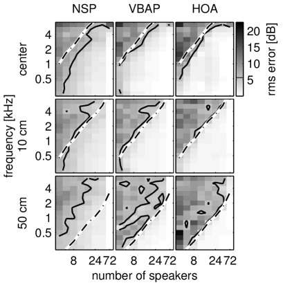
Figure 5: Beam pattern error as a function of frequency and number of loudspeakers, with a contour line for the 5.7 dB beam error criterion (solid line). Additionally, the HOA aliasing criterion (Eq. 6) for the ear with the largest distance to the center is marked by a dashed-dotted line. In the three top panels the listener was positioned in the center of the listening area. In the middle panels, the listener was moved 10 cm to the left side (corresponding to head movements), and in the bottom panels the listener was moved 0.5 m to the left side (corresponding to torso movements).

The exemplary beam patterns (Fig. 6) illustrate the differences in spatial interpolation between the three spatial reproduction methods. The effect of nearest neighbor sampling in the NSP method is obvious. However, VBAP interpolates only between two sources, which results in noncontinuous derivatives over the azimuth (e.g., sharp tips of the side lobes). With HOA the gain is continuously differentiable.

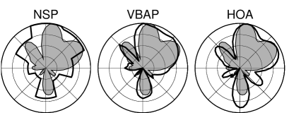
Figure 6: Exemplary beam pattern of the binaural beamformer, measured at 2 kHz with 8 loudspeakers using NSP (left panel), VBAP (center panel) and HOA (right panel). The shaded area denotes the beam pattern in the reference condition (free field).

3.2 SNR behavior of hearing aid algorithms

The SNR error (Eq. 10) of the four tested hearing aid algorithms in a simulated diffuse noise environment with 20 noise sources and a frontal target source is shown in Figures 7 to 10.

The SNR error of the binaural beamformer, Fig. 7, decreases with increasing number of loudspeakers and with decreasing frequency, similar to the beam error. The SNR error criterion of 0.75 dB is well predicted by the theoretical aliasing criterion Eq. 6, for VBAP and HOA. With NSP the SNR error criterion can only be reached up to 2 kHz even for large numbers of loudspeakers. In the 50 cm off-center listening position the SNR error is above the threshold also for low frequencies. For example, if 24 loudspeakers are available, the usable bandwidth in the central listening position is 2 kHz for NSP, 4 kHz for VBAP, and 5 kHz for HOA; in the 50 cm off-center listening position the same number of loudspeakers would lead to a usable bandwidth of 500 Hz with NSP, and 1 kHz with VBAP and HOA.

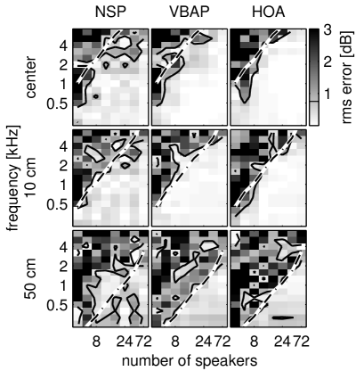
Figure 7: SNR error of the binaural beamformer as a function of frequency and number of loudspeakers, with a contour line for the SNR error criterion of 0.75 dB (solid line). In the three top panels the listener was positioned in the center of the listening area. In the middle panels, the listener was moved 10 cm to the left side (corresponding to head movements), and in the bottom panels the listener was moved 0.5 m to the left side (corresponding to torso movements).

The adaptive differential microphone, Fig. 8, shows a completely different SNR behavior: The SNR error is smallest for NSP; here it is below the threshold criterion of 0.3 dB at most frequencies and all listening positions as soon as more than 8 loudspeakers are used for reproduction. With HOA the SNR error criterion is similar to the spatial aliasing criterion of Eq. 6, limiting the usable bandwidth for low numbers of loudspeaker. With VBAP the performance is between NSP and HOA.

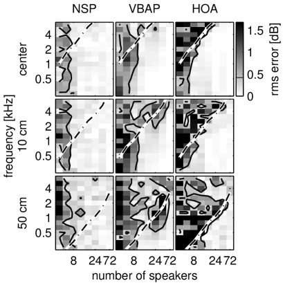
Figure 8: Same as Figure 7, but for the adaptive differential microphone, with an SNR error criterion of 0.42 dB.

The binaural noise reduction algorithm, Fig. 9, draws again a different picture: Here, the SNR error is more or less independent from the reproduction method. For the central listening position and the 10 cm off-center listening position the spatial aliasing criterion, Eq. 6, predicts the performance well for all reproduction methods. At low frequencies the SNR error is low in all conditions. This is caused by the fact that the algorithm has no significant effect on low frequency components, because the interaural coherence is always high. For example, to achieve a bandwidth of 2 kHz in the central listening position, 18 loudspeakers would be required for NSP and VBAP, and 12 for HOA. If for example 24 loudspeakers are available, the usable bandwidth is in central listening position 4 kHz for NSP and VBAP, and 6 kHz for HOA.

Figure 9: Same as Figure 7, but for the binaural noise reduction, with an SNR error criterion of 0.42 dB.

The SNR error of the single channel noise reduction, shown in Fig 10, shows a similar behavior as the binaural noise reduction scheme, even without any explicit spatial sensitivity. For VBAP and HOA the SNR error criterion is again approximated by the aliasing criterion. As a tendency also the SNR error criterion with NSP is predicted by the aliasing criterion. However, the SNR error shows now more frequency dependency than for the other tested algorithms, i.e., the effect of the number of loudspeakers used in the reproduction is smaller. The selection of reproduction method has no clear effect on the SNR error.

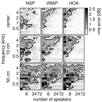
Figure 10: Same as Figure 7, but for the single channel noise reduction, with an SNR error criterion of 0.65 dB.

3.3 Perceptual model predictions

The perceptual localization error (PLE) in the three listening positions is shown in Figure 11. For NSP the PLE is half of the angular distance between the loudspeakers. In the central listening position HOA reproduces the DOA the best, with a negligible PLE starting with 8 loudspeakers. For off-center listening positions the PLE of HOA and VBAP increases, and is the same as for NSP in the 50 cm off-center listening position. The same ranking of errors can be observed when estimating the direction of arrival based on the envelope ITD in frequency bands above 1.3 kHz, see Figure 12.

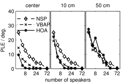
Figure 11: Perceptual localization error (PLE), as predicted by the perceptual binaural localization model of Dietz et al. (2011). The left panel shows data for the central listening position, the center and right panels for the listening position 0.1 m and 0.5 m to the left of the center, respectively. For NSP the PLE is half of the angular distance between the loudspeakers.

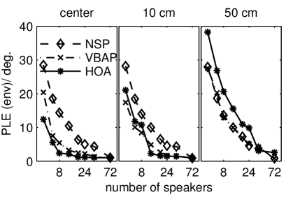
Figure 12: Same as Figure 11, but for the direction of arrival estimation based on the envelope in frequency bands above 1.3 kHz.

The perceptual spectral distance between the virtual sound source (reference) and the reproduced source is shown in Fig. 13. The test stimulus was the same speech signal as in the SNR measurements, see 2.3.2 for details. For NSP the distance is determined only by timbral changes caused by the spatial sampling of the HRIRs. For the other reproduction methods, also spectral changes caused by spatial aliasing contribute to an increased spectral distance.

All of the spectral distance values are below 0.25. A comparison with the subjective data provided by Moore and Tan (2004) indicates that even the largest spectral distance measured in this study corresponds to the highest rating of naturalness for speech.

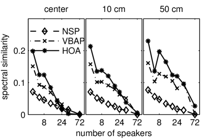
Figure 13: Monaural spectral distance, as predicted by the perceptual model of Moore and Tan (2004). Values of 0 correspond to no perceptual difference to the reference free-field condition. The data were averaged across all tested target directions from $-75$ to 75 degrees. Except for the central listening position with at least 18 loudspeakers, HOA produces the largest monaural quality degradation.

4 Discussion

When loudspeaker-based spatial audio reproduction methods are involved in the evaluation of hearing aids, the question arises to what extend the results are influenced by the reproduction methods. All reproduction methods have a physical limitation caused by the spatial aliasing, which means that above a certain frequency the reproduced signals contain spectral and spatial artifacts. The reproduction methods evaluated in this study represent a trade-off between minimal spectral artifacts and maximal spatial limitations (NSP) at one end, and maximal spectral artifacts combined with minimal spatial artifacts (HOA) on the other end of the scale. However, the picture is not that clear for hearing aid evaluations: Depending on the microphone positions and signal processing of the hearing aids, spatial artifacts can translate into spectral ones and vice versa. The SNR error of the single channel noise reduction (Fig. 10) may serve as an example: Although the algorithm uses only a single microphone, the error of the SNR performance measure follows more or less the spatial aliasing relation with all reproduction methods. Since the only input parameter to the algorithm is the frequency dependent short-time SNR, it can be concluded that spatial resolution can translate into spectral artifacts as soon as multiple virtual sources are involved.

It is well known from the literature that broadband signal to noise ratio is not directly related to speech intelligibility, e.g., single channel noise reduction often increases the SNR without any positive effect on speech intelligibility. Here, the broadband SNR is used as a differential algorithm performance measure. For a prediction of speech intelligibility, however, the SNR remains a major component. Commonly used models for speech intelligibility prediction are segmental SNR (Mermelstein, 1979), frequency weighted SNR (SII) (ANSI, 1997), or some form of signal-to-noise ratio after modeling the auditory periphery (Christiansen et al., 2010). The application of a much simpler broadband measure seems applicable in the context of this study, because not the absolute performance of the algorithms and their user benefit was of interest, but rather the validation of multichannel loudspeaker reproduction. If the tested reproduction methods are unable to reproduce the effect of algorithms on broadband SNR, it is likely that realistic speech intelligibility measurements would not be warranted either.

The threshold criteria for the instrumental measures of this study were derived from the distribution of the measured data, to allow a comparison with the theoretical spatial aliasing criterion. For the SNR-based measure, the resulting criteria are related to the maximal algorithm SNR benefit. For all algorithms, the threshold is in the range between 0.42 and 0.75 dB, which is comparable to the resolution of speech reception threshold measurements.

Multichannel loudspeaker audio reproduction methods may introduce several different artifacts. This study focuses only on artifacts which explicitly relate to hearing aid algorithm performance. This does not imply that other artifacts, such as reduced perceptual spatial resolution, increase of apparent source width, or head movement related time-varying coloration don’t have an effect on naturalness and immersion when listening with hearing aids. However, these classes of artifacts have been thoroughly described in the literature (e.g., Landone and Sandler, 1999; Daniel, 2001; Daniel et al., 2003; Carlsson, 2004; Pulkki and Hirvonen, 2005; Ahrens and Spors, 2008; Benjamin et al., 2010; Bertet et al., 2013; Heeren et al., 2014), and an in-depth analysis of these artifacts would go beyond the scope of this study.

For the purpose of this study, it was necessary to quantify any changes in technical algorithm performance induced by sound field approximations relative to the free sound field in a systematic, significant and sensitive way. It is therefore not claimed nor necessary that the applied instrumental measures reflect subjective performance, they only need to be sensitive to relative changes in algorithm performance induced by small changes of the sound field, in particular for speech sounds. The broadband SNR appears suitable for this purpose, as it is an established measure, integrates in a meaningful way across frequency and is robust against systematic small changes of the absolute transfer characteristics.

Different hearing aid algorithms are designed to provide benefit in different acoustic environments. Here, all algorithms were tested in only one diffuse noise environment. In other environments, the absolute benefit of algorithms might be different, and they might be more sensitive to the spatial resolution of the reproduction system; it remains to be studied to what extent the results in the diffuse noise environment may be generalized. The results indicate that besides some algorithm specific differences, the theoretic spatial aliasing criterion is a good first estimate for the effect on reproduction method performance. This suggests that the selection of the test environment was reasonable, and results may extent to other environments. Additionally, in the diffuse noise environment all of the tested algorithms are expected to provide some benefit, whereas in other environments, e.g., a single target with a single noise source, some algorithms are known to fail.

In this study only broadband spatial audio reproduction methods were tested. By the use of optimal reproduction methods in different frequency ranges the perceptual artifacts can be reduced at high frequencies, especially for off-center listening positions. This is common practice in HOA applications, where often ’basic’ decoding is applied at low frequencies, and ’max-rE’ decoding at higher frequencies (Daniel, 2001).

Here, instrumental performance measures were applied to the assessment of 2D audio reproduction. For plausibility of virtual environments, however, the technical precision of reproduction might be less important than a full immersion, as it would only be achieved by 3D audio reproduction. In hearing-aid research, however, most established evaluation procedures employ high-resolution 2D spatial setups and current algorithms mainly consider horizontal spatial properties, so that a compromise solution may be a mixed system with high horizontal resolution for sources which require high spatial resolution, and a low resolution 3D system primarily for immersion (e.g., Grimm et al., 2013; Grimm and Hohmann, 2014).

This study is based on simulations in a free sound field, as would be achievable by placing the loudspeaker array in an anechoic room. For practical applications, however, most systems would be located in regular rooms, optimally with some sound absorbing acoustic treatment. Accordingly it is of interest to know to what extent the results of the current study may be transferred to such real rooms. Obviously rooms with salient room resonances may create standing waves, which will reduce localization performance for any reproduction method. Also early lateral reflections and large amount of reverberation decrease localization performance, as was shown by Hartmann (1983). On the other hand, the monaural artifact of spectral coloration due to comb filter artifacts introduced by the VBAP and HOA reproduction methods in off-center listening positions, which is clearly perceivable in anechoic conditions when the listener is moving laterally, can be substantially masked by a moderate amount of room reverberation. All together, the main differences between the analyzed reproduction systems therefore will remain in real rooms. Appropriate acoustic treatment is recommended, particularly when physically correct reproduction is of importance.

5 Conclusions

All tested spatial reproduction methods are suitable for the assessment of hearing aid algorithm performance. However, the optimal system and its required number of loudspeakers depend on the type of hearing aid algorithm as well as on bandwidth requirements.

In tasks which require a high spatial resolution, such as an analysis of beam patterns of directional algorithms, higher order ambisonics and vector base amplitude panning performed best.

In tasks which analyze the SNR behavior of hearing aid algorithms the optimal reproduction method depends on the algorithm class: The performance of binaural noise reduction is largely independent of the reproduction method, and depends only on the number of loudspeakers and the listening position. The analysis of an adaptive differential microphone revealed that the theoretical free-field SNR behavior is best reproduced with the selection of the nearest speaker for each source. In that case the performance does not depend on the number of loudspeakers or listening position, if at least eight loudspeakers are used.

The theoretical free-field SNR behavior of a binaural beamformer is best reproduced in the central listening position by higher order ambisonics. Also perceptual localization performance in the central listening position is best reproduced by higher order ambisonics – here the deviation from free field simulation is negligible even with only eight loudspeakers. However, for off-center listening positions the advantage of higher order ambisonics vanishes.

The data also show that care has to be taken in selecting the appropriate reproduction method even when only algorithms are involved that do not explicitly depend on spatial sound field properties, such as single channel noise reduction. Furthermore, it can be concluded that even the selection of discrete speakers, which is free of spatial aliasing for a single source, can lead to typical spatial aliasing artifacts when multiple sources are reproduced.

As a rough guideline the data can be summarized as follows:

• With fewer than eight loudspeakers, the performance measure criteria are not matched for most tested conditions.

• For a beam pattern analysis and 4 kHz bandwidth, 18 loudspeakers are required in the central listening position (no head movements), 36 loudspeakers are required in 10 cm off-center listening position (head movements allowed), and 72 loudspeakers are required in the 50 cm off-center listening position (head- and torso movements allowed). For a beam pattern analysis, VBAP and HOA appear to be the best choice.

• The SNR behavior of the adaptive differential microphone (ADM) in complex acoustic scenarios is best reproduced with discrete speakers (NSP) in all listening positions. Using more than 8 loudspeakers does not provide any benefit in this condition.

• The SNR behavior of single channel noise reduction is best reproduced using VBAP or HOA. This indicates that spatial audio reproduction methods which interpolate between loudspeakers can be beneficial even for hearing aid algorithms which do not explicitly depend on spatial properties of the sound field.

References

- Ahrens and Spors (2008) J. Ahrens and S. Spors. An analytical approach to sound field reproduction using circular and spherical loudspeaker distributions. Acta Acustica united with Acustica, 94(6):988–999, 2008.
- ANSI (1997) ANSI. Methods for the calculation of the speech intelligibility index. American National Standard S3.5–1997, Standards Secretariat, Acoustical Society of America, 1997.
- Bates et al. (2007) E. Bates, G. Kearney, F. Boland, and D. Furlong. Monophonic source localization for a distributed audience in a small concert hall. In Proc. of the 10th Int. Conference on Digital Audio Effects (DAFx-07), Bordeaux, France, September 2007.
- Benjamin et al. (2010) E. Benjamin, A. Heller, and R. Lee. Why ambisonics does work. In Audio Engineering Society Convention 129, 11 2010. URL http://www.aes.org/e-lib/browse.cfm?elib=15664.
- Bentler (2005) R. A. Bentler. Effectiveness of directional microphones and noise reduction schemes in hearing aids: A systematic review of the evidence. Journal of the American Academy of Audiology, 16(7):473–484, 2005. doi: doi:10.3766/jaaa.16.7.7.
- Berkhout et al. (1993) A. J. Berkhout, D. de Vries, and P. Vogel. Acoustic control by wave field synthesis. The Journal of the Acoustical Society of America, 93(5):2764–2778, 1993. doi: 10.1121/1.405852.
- Bertet et al. (2013) S. Bertet, J. Daniel, E. Parizet, and O. Warusfel. Investigation on localisation accuracy for first and higher order ambisonics reproduced sound sources. Acta Acustica united with Acustica, 99(4):642–657, 2013.
- Brandenburg et al. (2004) K. Brandenburg, S. Brix, and T. Sporer. Wave field synthesis: From research to applications. In Proceedings of 12th European Signal Processing Conference (EUSIPCO), Vienna, Austria, 2004.
- Carlsson (2004) K. Carlsson. Objective Localisation Measures in Ambisonic Surround-sound. PhD thesis, Master Thesis in Music Technology, Supervisor: Dr. Damian Murphy. Department of Speech, Music and Hearing, Royal Institute of Technology, Stockholm. Work carried out at Dept. of Electronics University of York, 2004.
- Christiansen et al. (2010) C. Christiansen, M. S. Pedersen, and T. Dau. Prediction of speech intelligibility based on an auditory preprocessing model. Speech Communication, 52(7-8):678 – 692, 2010. ISSN 0167-6393.
- Cord et al. (2004) M. Cord, R. Surr, B. Walden, and O. Dyrlund. Relationship between laboratory measures of directional advantage and everyday success with directional microphone hearing aids. Journal of the American Academy of Audiology, 15(5):353–364, 2004.
- Daniel (2001) J. Daniel. Représentation de champs acoustiques, application à la transmission et à la reproduction de scènes sonores complexes dans un contexte multimédia. PhD thesis, Université Pierre et Marie Curie (Paris VI), Paris, 2001.
- Daniel et al. (2003) J. Daniel, R. Nicol, and S. Moreau. Further investigations of high-order ambisonics and wavefield synthesis for holophonic sound imaging. In Audio Engineering Society Convention 114, March 2003.
- Dietz et al. (2011) M. Dietz, S. D. Ewert, and V. Hohmann. Auditory model based direction estimation of concurrent speakers from binaural signals. Speech Communication, 53(5):592 – 605, 2011. ISSN 0167-6393. doi: 10.1016/j.specom.2010.05.006.
- Elko and Pong (1995) G. W. Elko and A.-T. N. Pong. A simple adaptive first-order differential microphone. Workshop on Applications of Signal Processing to Audio and Acoustics, pages 169 – 172, 1995.
- Eneman et al. (2008) K. Eneman, A. Leijon, S. Doclo, A. Spriet, M. Moonen, and J. Wouters. Advances in Digital Speech Transmission, chapter Auditory-Profile-Based Physical Evaluation of Multi-Microphone Noise Reduction Techniques in Hearing Instruments. John Wiley and Sons, Ltd, 2008.
- Ephraim and Malah (1984) Y. Ephraim and D. Malah. Speech enhancement using a minimum-mean square error short-time spectral amplitude estimator. IEEE Transactions on Acoustics, Speech and Signal Processing, 32(6):1109–1121, 1984.
- Favrot and Buchholz (2009) S. Favrot and J. Buchholz. Validation of a loudspeaker-based room auralization system using speech intelligibility measures. In 126th Audio Engineering Society convention, 2009.
- Favrot and Buchholz (2010) S. Favrot and J. M. Buchholz. LoRA: A Loudspeaker-Based room auralization system. Acta Acustica united with Acustica, 96(2):364–375, 2010.
- Greenberg et al. (2003) J. E. Greenberg, J. G. Desloge, and P. M. Zurek. Evaluation of array-processing algorithms for a headband hearing aid. The Journal of the Acoustical Society of America, 113(3):1646–1657, 2003.
- Grimm and Hohmann (2014) G. Grimm and V. Hohmann. Dynamic spatial acoustic scenarios in multichannel loudspeaker systems for hearing aid evaluations. In 17. Jahrestagung der Deutschen Gesellschaft für Audiologie, Oldenburg, Germany, 2014. Deutschen Gesellschaft für Audiologie.
- Grimm et al. (2006) G. Grimm, T. Herzke, D. Berg, and V. Hohmann. The Master Hearing Aid – a PC-based platform for algorithm development and evaluation. 92:618–628, 2006.
- Grimm et al. (2009) G. Grimm, V. Hohmann, and B. Kollmeier. Increase and subjective evaluation of feedback stability in hearing aids by a binaural coherence based noise reduction scheme. IEEE Transactions on Audio, Speech and Language Processing, 17(7):1408–1419, September 2009.
- Grimm et al. (2013) G. Grimm, G. Coleman, and V. Hohmann. Realistic spatially complex acoustic scenes for space-aware hearing aids and computational acoustic scene analysis. In 16. Jahrestagung der Deutschen Gesellschaft für Audiologie, Rostock, Germany, 2013. Deutschen Gesellschaft für Audiologie.
- Guastavino and Katz (2004) C. Guastavino and B. F. G. Katz. Perceptual evaluation of multi-dimensional spatial audio reproduction. The Journal of the Acoustical Society of America, 116:1105, 2004.
- Hamacher et al. (2005) V. Hamacher, J. Chalupper, J. Eggers, E. Fischer, U. Kornagel, H. Puder, and U. Rass. Signal processing in high-end hearing aids: state of the art, challenges, and future trends. EURASIP Journal on Applied Signal Processing, 2005:2915–2929, 2005.
- Hamasaki (2011) K. Hamasaki. 22.2 multichannel audio format standardization activity. Broadcast Technology, (45), 2011.
- Hamasaki et al. (2005) K. Hamasaki, K. Hiyama, and R. Okumura. The 22.2 multichannel sound system and its application. In Audio Engineering Society Convention 118, May 2005. URL http://www.aes.org/e-lib/browse.cfm?elib=13122.
- Hartmann (1983) W. M. Hartmann. Localization of sound in rooms. The Journal of the Acoustical Society of America, 74(5):1380–1391, 1983.
- Heeren et al. (2014) J. Heeren, G. Grimm, and V. Hohmann. Evaluation of an ambisonics system for psychoacoustical measurements in non-anechoic conditions. In Biomed Tech, volume 59, 2014. doi: DOI 10.1515/bmt-2014-5011.
- ITU-R (2012) ITU-R. Recommendation itu-r bs.775-3: Multichannel stereophonic sound system with and without accompanying picture. Broadcasting service (sound), 2012.
- Kates (2008) J. M. Kates. Digital hearing aids. Plural Pub., 2008.
- Kayser et al. (2009) H. Kayser, J. Anemüller, T. Rohdenburg, V. Hohmann, B. Kollmeier, et al. Database of multichannel in-ear and behind-the-ear head-related and binaural room impulse responses. EURASIP Journal on Advances in Signal Processing, 2009.
- Kollmeier et al. (1993) B. Kollmeier, J. Peissig, and V. Hohmann. Binaural noise-reduction hearing aid scheme with real-time processing in the frequency domain. Scand Audiol, Suppl. 38:28–38, 1993.
- Landone and Sandler (1999) C. Landone and M. Sandler. Issues in performance prediction of surround systems in sound reinforcement applications. In Proceedings of the 2nd COST G-6 Workshop on Digital Audio Effects (DAFx99), Norwegian University of Science and Technology, Trondheim, Norway, December 1999.
- Luo et al. (2002) F.-L. Luo, J. Yang, C. Pavlovic, and A. Nehorai. Adaptive null-forming scheme in digital hearing aids. IEEE Transactions on signal processing, 50(7):1583–1590, 2002.
- Luts et al. (2010) H. Luts, K. Eneman, J. Wouters, M. Schulte, M. Vormann, M. Buechler, N. Dillier, R. Houben, W. A. Dreschler, M. Froehlich, H. Puder, G. Grimm, V. Hohmann, A. Leijon, A. Lombard, D. Mauler, and A. Spriet. Multicenter evaluation of signal enhancement algorithms for hearing aids. The Journal of the Acoustical Society of America, 127(3):1491–1505, 2010. doi: 10.1121/1.3299168. URL http://link.aip.org/link/?JAS/127/1491/1.
- Mermelstein (1979) P. Mermelstein. Evaluation of a segmental snr measure as an indicator of the quality of adpcm coded speech. The Journal of the Acoustical Society of America, 66(6):1664–1667, 1979.
- Moore and Tan (2004) B. C. J. Moore and C.-T. Tan. Development and validation of a method for predicting the perceived naturalness of sounds subjected to spectral distortion. J. Audio Eng. Soc, 52(9):900–914, 2004. URL http://www.aes.org/e-lib/browse.cfm?elib=13018.
- Nettingsmeier (2010) J. Nettingsmeier. General-purpose ambisonic playback systems for electroacoustic concerts - a practical approach. In Proc. of the 2nd International Symposium on Ambisonics and Spherical Acoustics, Paris, France, May 2010.
- Neukom (2007) M. Neukom. Ambisonic panning. In Audio Engineering Society Convention 123, 10 2007. URL http://www.aes.org/e-lib/browse.cfm?elib=14354.
- Olaiz et al. (2009) N. Olaiz, P. Arumı, T. Mateos, and D. Garcia. 3d-audio with clam and blender’s game engine. In Linux Audio Conference, 2009.
- Oreinos et al. (2013) C. Oreinos, J. M. Buchholz, and J. Mejia. Effect of higher-order ambisonics on evaluating beamformer benefit in realistic acoustic environments. In Applications of Signal Processing to Audio and Acoustics (WASPAA), 2013 IEEE Workshop on, pages 1–4. IEEE, 2013.
- Pulkki (1997) V. Pulkki. Virtual sound source positioning using vector base amplitude panning. J. Audio Eng. Soc, 45(6):456–466, 1997.
- Pulkki and Hirvonen (2005) V. Pulkki and T. Hirvonen. Localization of virtual sources in multichannel audio reproduction. Speech and Audio Processing, IEEE Transactions on, 13(1):105–119, 2005.
- Rohdenburg et al. (2007) T. Rohdenburg, V. Hohmann, and B. Kollmeier. Robustness analysis of binaural hearing aid beamformer algorithms by means of objective perceptual quality measures. In Applications of Signal Processing to Audio and Acoustics, 2007 IEEE Workshop on, pages 315–318. IEEE, 2007.
- Seeber et al. (2010) B. U. Seeber, S. Kerber, and E. R. Hafter. A system to simulate and reproduce audio–visual environments for spatial hearing research. Hearing research, 260(1):1–10, 2010.
- Smeds et al. (2006) K. Smeds, G. Keidser, J. Zakis, H. Dillon, A. Leijon, F. Grant, E. Convery, and C. Brew. Preferred overall loudness. ii: Listening through hearing aids in field and laboratory tests. International Journal of Audiology, 45(1):12–25, 2006.
- Solvang (2008) A. Solvang. Spectral impairment of two-dimensional higher order ambisonics. Journal of the Audio engineering Society, 56(4):267–279, 2008.
- Spors et al. (2008) S. Spors, R. Rabenstein, and J. Ahrens. The theory of wave field synthesis revisited. In 124th AES Convention, 2008.
- Spriet et al. (2005) A. Spriet, M. Moonen, and J. Wouters. Robustness analysis of multichannel wiener filtering and generalized sidelobe cancellation for multimicrophone noise reduction in hearing aid applications. Speech and Audio Processing, IEEE Transactions on, 13(4):487–503, 2005.
- Tessendorf et al. (2011) B. Tessendorf, A. Kettner, D. Roggen, T. Stiefmeier, G. Tröster, P. Derleth, and M. Feilner. Identification of relevant multimodal cues to enhance context-aware hearing instruments. In Proceedings of the 6th International Conference on Body Area Networks, pages 15–18. ICST (Institute for Computer Sciences, Social-Informatics and Telecommunications Engineering), 2011.
- Widrow and Luo (2003) B. Widrow and F.-L. Luo. Microphone arrays for hearing aids: An overview. Speech Communication, 39(1):139–146, 2003.
- Wittkop and Hohmann (2003) T. Wittkop and V. Hohmann. Strategy-selective noise reduction for binaural digital hearing aids. Speech Communication, 39:111–138, 2003.
- Wittkop et al. (1997) T. Wittkop, S. Albani, V. Hohmann, J. Peissig, W. S. Woods, and B. Kollmeier. Speech processing for hearing aids: Noise reduction motivated by models of binaural interaction. Acta Acustica united with Acustica, 83(4):684–699, 1997.