Magnetic order and superconductivity observed in bundles of Double-Wall Carbon Nanotubes

Abstract

The magnetotransport properties were studied in hundreds of micrometer length double-wall carbon nanotubes (DWCNT) bundles. Above 15 K the resistance shows an ohmic behavior and its temperature dependence is well described using the variable-range hopping for one-dimensional system. The magnetoresistance is negative and can be explained using an empirical model based on spin-scattering processes indicating the existence of magnetic order up to room temperature. At temperatures between 2 K and 15 K the resistance is non-ohmic and the current-voltage characteristics reveal the appearance of a potential, which can be well described by a fluctuation-induced tunneling conduction model. In this low temperature range and at low enough input current, a positive magnetoresistance appears - in addition to the negative one - with an extraordinary hysteresis in field and vanishes at $T\sim 15~{}$K, suggesting the existence of a superconducting state. Magnetization results partially support the existence of both phenomena in the DWCNT bundles.

1 Introduction

The search for superconductivity and magnetic order in carbon-based materials triggered a large number of studies in recent years. Experimental as well as theoretical works indicate that magnetic order at high temperatures in graphite is possible through the influence of vacancies and/or hydrogen (for recent reviews see [1, 2] and refs. therein). In contrast to graphite and in spite of theoretical predictions on the possibility to have magnetic order due to hydrogen or vacancies in carbon nanotubes (CNT) [3, 4, 5], the observation of this phenomenon in these carbon structures appears to be more difficult. Apparently, only the hydrogenated CNT prepared in [6, 7] showed the existence of magnetic order at room temperature. However, and in clear contrast, several studies reported the existence of superconductivity through measurements in single nanotubes as well as bundles of them (single- and multiwall) [8, 9, 10, 11, 12, 13, 14, 15]. Apparently, the critical temperature obtained for the CNT depends on the sample and the experimental method used; it ranges between $\sim 0.5~{}$K to $\sim 15~{}$K.

The origin of the observed superconductivity in CNT is still under debate. Maxima in the electronic density of states, called van Hove singularities, have been used as possible origin for the superconducting-like signals measured after application of a gate voltage [15], purely electronic mechanism in certain geometries of ultra-small diameter ($\lesssim 2~{}$nm) [16], an overwhelming attractive electron-phonon interaction in double-wall CNT (DWCNT) specially when the outer tube is metallic [17], are some of the theoretical concepts one finds nowadays in recent studies predicting superconductivity in CNT.

In this experimental work, we studied the electrical transport properties of bundles of, mostly, DWCNT as a function of temperature and magnetic field. The observed negative magnetoresistance of the CNT-bundle in the whole temperature range indicates the existence of spin dependent scattering processes up to room temperature, similar to that found in materials with defect-induced magnetism (DIM), see e.g. [18]. We found that an extra contribution to the magnetoresistance appears at $T<15~{}$K and at low enough input currents. This fact and the observed positive magnetoresistance with its hysteretic behavior suggest the existence of superconductivity in a similar temperature range as the one found recently in DWCNT [11] as well as in pyrolytic graphite flakes under an electric field [19]. The temperature dependence of the magnetization, its hysteresis and other features support also the existence of magnetic order and to some extent of superconductivity.

2 Experimental details

2.1 Carbon Nanotubes Synthesis

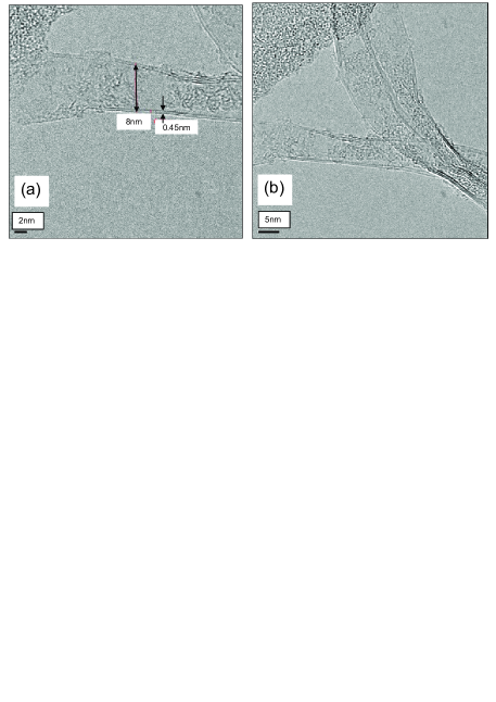
Figure 1: Transmission electron pictures of the measured DWCNT.

The used procedure to synthesize the CNT was the following: The wafers for the growth substrates were prepared by e-beam evaporation (base pressure between $7\times 10^{-7}$ and $2\times 10^{-6}~{}$Torr) where 1.2 nm Fe and 10 nm Al₂O₃ films were deposited on 4 inches diameter silicon wafers. The gases used for the carbon nanotubes (CNT) growth were Ar (99.9995%, Maxima), C₂H₄ (99.5%, Maxima), H₂ (99.999%, Maxima), and a mixture of 99% Ar with 1% oxygen, which we will denote as Ar/O₂ (Maxima). The flows were maintained using electronic mass flow controllers (MKS, model 1179A). The experiment was performed on 0.5 cm² catalyst substrates and with the same gas preheating and fast heating techniques previously described [20, 21]. The synthesis were performed using a fused-silica tube (internal diameter of 22 mm) placed in two atmospheric-pressure tube furnaces (Lindberg Blue) with controlled flows of the source gases - Ar, H₂, C₂H₄, and Ar/O₂. The first furnace (set at 770 ^∘C) preheated the gases. The growth substrate was positioned in the second furnace (at 755^∘C) for the annealing and growth steps. The substrate were inserted into the furnace for a 15 minutes anneal with 100 sccm of Ar and 400 sccm of H₂, followed by a 30 minutes growth cycle with 100 sccm of Ar, 100 sccm of Ar/O₂, 400 sccm of H₂ and 200 sccm of C₂H₄. At the end of CNT growth, the H₂ and C₂H₄ were turned off and the substrate was post-annealed in the remaining Ar and Ar/O₂ for 2 minutes. Then the Ar/O₂ gas was turned off, and H₂ gas was turned on for an additional minute of anneal. Then the H₂ gas was turned off, and the sample was removed from the heated zone and positioned above a cooling fan (with Ar still flowing within the tube) until it was cool enough to be removed for characterization.

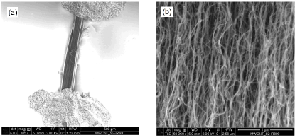
Figure 2: (a) Scanning electron microscope (SEM) picture of one of the measured bundles with the voltage electrodes. The scale bar is 500 $\mu$m. (b) SEM picture with higher resolution of the CNT bundle. The scale bar is 1 $\mu$m.

2.2 Characterization methods

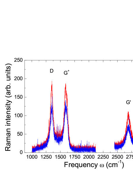
Figure 3: Raman spectra obtained at two different positions of a DWCNT bundle (blue and red curves).

The morphology of the CNT was examined using scanning electron microscopy (SEM, Quanta FEG 250), high-resolution transmission electron microscopy (HRTEM, Jeol 2010) and a dual beam microscope NovaLab XT200 from FEI. Figure 1 shows two TEM pictures where we can recognize the double-wall and the diameter of the CNT. Figure 2 shows scanning electron microscope (SEM) pictures of the measured bundles with the voltage-current electrodes at the edges (a). In Fig. 2(b) we can recognize that most of the CNT are connected. Although we could not measure directly the transport response of a single interconnection, we speculate that these may have some contribution on the observed behavior we describe below. Information about the elemental composition of the bundles was obtained from energy dispersive X-ray (EDX) analysis. Any traces of magnetic elements like Fe, Ni, etc., were below the experimental resolution of 50 ppm. However, from recently published studies [22] we know that EDX analysis is not really appropriate to find and characterize traces of magnetic impurities embedded in carbon-based materials. Therefore a further characterization of the magnetic impurities has been made using particle induced x-ray emission (PIXE), a method that provides better resolution and other advantages in comparison to EDX [22]. The PIXE results indicate the existence of Fe dispersed within the bundle of DWCNT with a concentration $\lesssim 250~{}\pm 50~{}\mu$g Fe per gram of carbon, a concentration equivalent to $\lesssim 60~{}\pm 15~{}$ppm Fe. This concentration is not relevant for electrical transport measurements, because the small amount of Fe-based grains are dispersed and likely attached either at some of the edges and/or at the surface of the DWCNT. However, if this Fe concentration shows magnetic order, it might provide a clear contribution to the total magnetization of the bundles and will be taken into account in the discussion. The concentration of other magnetic impurities is more than one order of magnitude below that of Fe and therefore not relevant for the interpretation of the results.

Micro-Raman spectrum was obtained at room temperature and ambient pressure with a Dilor XY 800 spectrometer at 514.53 nm wavelength and a 2 $\mu$m spot diameter. The incident power was kept at 1.5 mW to avoid any sample damage or laser induced heating effects. The Raman spectra obtained at two different positions of a bundle of CNT are shown in Fig. 3. The spectra show many peaks; as in graphite and single wall carbon nanotubes (SWCNT) a D band peak (at $\simeq 1350~{}$cm^-1), the G⁺ peak (around 1580 cm^-1, also observed in semiconducting SWCNT [23]), the overtone of the D peak, named G’ (at $\simeq 2690~{}$cm^-1) and also observed in semiconducting SWCNT [23] and an overtone longitudinal optic (LO, at $\simeq 2940~{}$cm^-1) peak. For our bundles we observe a G⁺/D ratio of approximately 1, which is indicative of defective CNT. This is consistent with the morphology observed in the SEM/TEM images.

For the electrical resistance measurements we separated carefully bundles of CNT with length of $\sim 800~{}\mu$m using non-magnetic tweezers. Afterwards the bundle was placed on the top of a $5\times 5~{}$mm² silicon (100) substrate covered with a 150-nm insulating Si₃N₄ film. The contacts for the resistance measurements were done using a commercial silver paste and gold wires (25 $\mu$m diameter) in a four-two points configuration (see Fig 2(a)). We have done also measurements with the usual four points to check whether the contact resistance contributed. The results were similar for both, four-two or four points configurations. The temperature dependence measurements were done in a commercial ⁴He-flow cryostat (Oxford Instruments) equipped with a superconducting magnet with maximal field $\pm 8~{}$T. During the measurements the magnetic field was applied perpendicular to the bundle main length. High resolution resistance measurements were done using an AC Bridge (Linear Research LR-700) in the range of temperature between 2 and 275 K. The temperature stabilization was better than 4 mK in the whole temperature range. For the current-voltage ($I-V$) measurements we used a Keithley DC and AC current source (Keithley 6221) and a nanovoltmeter (Keithley 2182). For the magnetization measurements we took a CNT-bundle of mass 1.0 mg and fixed it with grease in the middle of a 13.5 cm long previously characterized pure quartz rod with negligible background [24]. The magnetic moment of the sample was measured using a superconducting quantum interference device magnetometer (SQUID) from Quantum Design.

3 Results and discussion

3.1 Temperature dependence of the resistance and nonlinear response at zero applied field

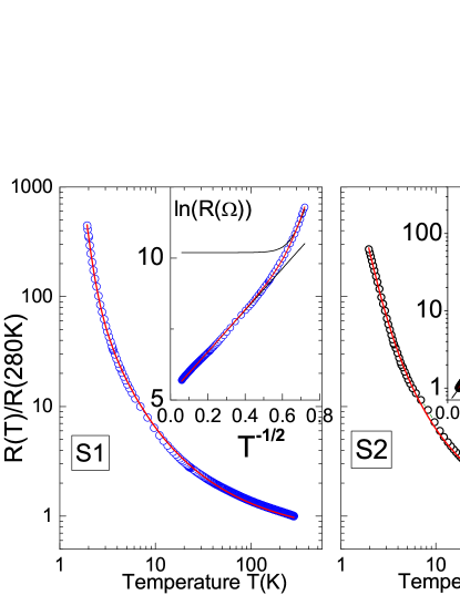
Figure 4: Normalized resistance vs. temperature for two samples, S1 (a) and S2 (b) at zero applied field and with an input current of $10~{}\mu$A. The inset in (a) shows the natural logarithm of the absolute resistance (in Ohms) vs. the inverse square root of the temperature. The inset in (b) shows the normalized resistance vs. $T^{-1/2}$ in semilogarithmic scale. The red lines in the main panels and insets are a fit to Eq. (5), which is the addition of the two contributions given by Eqs. (1,2), the two black lines in the inset of (a).

We have investigated in total five samples, which showed similar behavior. Therefore, we discuss here the results obtained for two of the samples, S1 and S2. Figure 4 shows the resistance as a function of temperature for the two samples. The insets show the same data but vs. $T^{-1/2}$. In the insets we recognize that the temperature dependence shows two different regions, one below and the other above $T\sim 10~{}$K. At temperatures above $\sim 10~{}$K, the resistance can be well described by the variable range hopping theory. In general, the resistance in the variable range hopping (VRH) regime can be expressed as:

$$R_{\rm VRH}(T)=R_{0}\exp((T_{H}/T)^{1/(1+d)})\,,$$ (1)

where $R_{0}$ is a free prefactor, $T_{H}$ is a characteristic temperature coefficient, and $d$ the dimensionality. In the case an energy gap is present at the Fermi Level, the VRH resistance follows $d=1$ as derived by Efros-Shklovskii [25]; for this special case $T_{H}=2.8e^{2}/\xi k_{B}\epsilon$, where $\epsilon$ is the dielectric constant, $e$ the elementary charge of the electron, $\xi$ a localization length and $k_{B}$ the Boltzmann constant. The insets in Fig. 4 indicate that the resistance of the CNT bundles follows a VRH mechanism (straight lines in those insets) above $T\sim 10~{}$K.

The low temperature part of the resistance can be understood using the fluctuation-induced tunneling (FIT) model, which considers metallic-like grains separated by insulating, tunneling barriers with an effective capacitance [26, 27]. According to the FIT model and at small applied electric fields (or currents), the temperature dependent resistance across a single, small junction is given by:

$$R_{\rm FIT}(T)=R_{A}\exp(T_{1}/(T_{0}+T))\,,$$ (2)

where

$$T_{1} = \frac{8\epsilon_{0}}{e^{2}k_{B}}\left(\frac{A\phi_{0}^{2}}{w}\right)\,,$$ (3)

$$T_{0} = \frac{16\epsilon_{0}\hbar}{\pi\sqrt{(2m)}e^{2}k_{B}}\left(\frac{A\phi_{0}^{3/2}}{w^{2}}\right)\,,$$ (4)

where $R_{A}$ is a parameter that depends weakly on temperature, $\phi_{0}$ is the barrier height, $w$ a barrier width and $A$ its lateral area, which is the effective geometrical area at the contact between the two metallic regions, $\epsilon_{0}$ the vacuum permittivity, and $m$ the electronic mass. The characteristic temperature $T_{1}$ can be interpreted as the energy required for an electron to cross the barrier $\phi_{0}$ and $T_{0}$ a temperature, well below which, thermal fluctuation effects become negligible.

We found that the simple addition of these two mechanisms, i.e. assuming the two resistances in series

$$R(T)=R_{\rm VRH}(T)+R_{\rm FIT}(T)\,,$$ (5)

fits the experimental data, as shown by the continuous curves through the experimental points obtained at $I=10~{}\mu$A , see Fig. 4. The parameters that fit the experimental data have some correlations and therefore should be given within some confidence range. Similar curves as shown in Fig. 4 can be obtained compensating the effects of the parameters within the following range: $R_{0}\simeq 180\pm 10~{}\Omega$, $T_{H}\simeq 50\pm 5~{}$K, $R_{A}=1\ldots 10~{}\Omega$, $10\lesssim T_{1}\lesssim 30~{}$K and $0.5\lesssim T_{0}\lesssim 2~{}$K.

Taking into account the SEM pictures, see Fig. 2, we expect that the electric current is not being transported by the same single CNT all along the electrodes but most of them are interconnected having junctions. In this case the resistance will be the sum of the two contributions, one from the 1D transport through the CNT and the other through the junctions in series. It is important to note that the FIT model implies that a nonlinear contribution to the ohmic resistance should exist. This contribution is given by a current-voltage characteristic of the type:

$$I_{\rm FIT}(V,T)=I_{0}\exp\left[-\frac{T_{1}}{T_{0}+T}\left(1-\frac{V}{V_{0}}\right)^{2}\right]\,,$$ (6)

where $V_{0}$ is a critical voltage. The measured current-voltage $(I-V)$ characteristic curves, see Fig. 5, show indeed such a nonlinear behavior that vanishes at $T\gtrsim 10~{}$K. Note the perfect symmetry of the $I-V$ curves for both signs of the applied current, in contrast to the $I-V$ behavior observed in single CNT junctions [28]. On the other hand, the nonlinearity of our $I-V$ curves at $T\lesssim 10~{}$K is similar to that observed in ropes of SWCNT in the same temperature range [29].

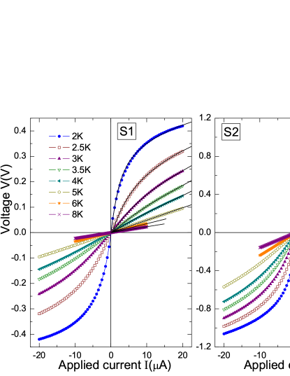
Figure 5: Voltage-current ($V-I$) characteristic curves measured for samples S1 and S2 at different constant temperatures and at zero applied field. The continuous lines through the experimental data are fits to the function given by Eq. (7).

The experimental $I-V$ curves can be fitted adding the contribution from the FIT model, Eq. (6), plus an ohmic term $I_{l}=V/R_{l}$ ($R_{l}$ is an ohmic resistance), which corresponds to the electrical paths without barriers:

$$I=I_{\rm FIT}(V,T)+(V/R_{l}(T))\,.$$ (7)

Figure 5 shows the measured $I-V$ curves for samples S1 and S2 at different constant temperatures. The continuous lines through the experimental data were calculated following Eq. (7) with parameters similar to those used to fit the temperature dependence of the resistance, see Fig. 4. Within the confidence range of the fit parameters $T_{1}$ and $T_{0}$ and Eqs. (3,4) we can estimate the width $w$ and area $A$ ranges of the junctions. Assuming $\phi_{0}\sim 0.1~{}$eV (see Fig. 5), we obtain $2.4~{}$nm $\lesssim w\lesssim 24~{}$nm, and $5\times 10^{-19}~{}$m² $\lesssim A\lesssim 1.5\times 10^{-17}~{}$m², values that indicate junctions of several nm length and width. The values and the spread of the fit parameters obtained using the FIT model are similar to those found in the literature [30, 31].

3.2 Magnetotransport properties

3.2.1 Negative magnetoresistance: Magnetic order contribution

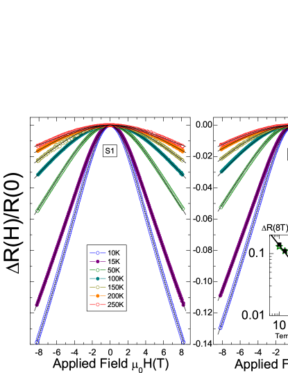
Figure 6: Magnetoresistance for samples S1 and S2 (right panel) as a function of magnetic field applied normal to the main axis of the CNT bundles, with a current of $10~{}\mu$A and at different constant temperatures. The inset in the right panel shows the magnetoresistance at a fixed field of 8 T vs. temperature in a double logarithmic scale. The straight line follows $0.63T^{-2/3}$.

The measurements of the magnetoresistance (MR) were done at different applied currents. At temperatures $T\gtrsim 15~{}$K, where the VRH behaviour of the resistance overwhelms (see Fig. 4), the magnetoresistance does not depend on the applied current for $I\lesssim 20~{}\mu$A, the maximum current applied in these studies. In this temperature range the MR is negative and rather large at low temperatures, see Fig. 6. Its field dependence can be fitted with the model proposed by Khosla and Fischer [32] that combines negative and positive magnetoresistances in semiconductors, taking into account a third-order expansion of the $s-d$ exchange Hamiltonian. The semiempirical formula for the magnetoresistance, defined as $\Delta R/R(0)=(R(H)-R(0))/R(0)$ as a function of the applied field $H=B/\mu_{0}$, is

$$\frac{\Delta R}{R(0)}=-a^{2}\ln(1+b^{2}B^{2})+\frac{c^{2}B^{2}}{1+d^{2}B^{2}}\,,$$ (8)

where $c$ and $d$ are free parameters that depend on the conductivity and the carrier mobility $\mu$, and

$$a^{2}=A_{1}J\rho_{F}[S(S+1)+\langle{M^{2}}\rangle]\,,$$ (9)

$$b^{2}=\left[1+4S^{2}\pi^{2}\left(\frac{2J\rho_{F}}{g}\right)^{4}\right]\frac{g^{2}\mu^{2}}{(\alpha kT)^{2}}\,,$$ (10)

where $\alpha$ is a constant. The parameters $a$ and $b$ in Eq. (8) depend on several factors such as a spin scattering amplitude $A_{1}$, the exchange integral $J$, the density of states at the Fermi energy $N(E_{F})$, the spin of the localized magnetic moments $S$ and the average magnetization square $\langle{M^{2}}\rangle$. The negative first term in Eq. (8) is the term attributed to a spin dependent scattering in third order ($s-d$ in usual $d-$band ferromagnets, $s-p$ in $p-$band ferromagnets [33]) exchange Hamiltonian. The positive second term in Eq. (8) is a Lorentz-like term that saturates at high fields and takes into account field induced changes due to the two conduction bands with different conductivities.

The fits of the experimental data to Eq. (8) for the two samples are shown in Fig. 6. Although the data can be well fitted with this model at all measured temperatures, the correlation and compensation effects between the four free parameters is too large to obtain reliable values of the intrinsic parameters of Eqs. (9) and (10). Instead, we show in the inset of Fig. 6 the MR at a fixed field of 8 T as a function of temperature for the two samples. The MR follows very well a $T^{-2/3}$ law at $T<200~{}$K. This dependence suggests that $<M^{2}(T)>\propto T^{-2/3}$, neglecting the change in temperature from the parameter $b(T)$ inside the logarithmic function in Eq. (9) and the weak contribution of the second term in Eq. (8). It is reasonable to assume that this has the same DIM origin as in graphite or nominally non-magnetic oxides [2]. In the case of bulk graphite the dependence of the ferromagnetic magnetization at fixed fields follows a nearly linear and negative $T$-dependence, i.e. $M(T)\sim M(0)(1-aT)$ [34, 35]. The obtained dependence deviates clearly from that observed in graphite, probably reflecting the different dimensionality of the magnetic order in the CNT.

We would like to emphasize that the contribution of the very small amount of magnetic impurities is unlikely to affect the magnetoresistance results. The detected $\simeq 60~{}$ppm Fe-containing grains would be some at the edges and some at the surface of the DWCNT. Therefore the main measured voltage due to the input current should not be influenced by the impurity grains. If we compare the case of CNT fully filled with conducting 35 nm diameter Fe reported recently [36], the temperature dependence of the negative magnetoresistance at a fixed field is completely different. It remains rather constant between 2 K and 100 K and sharply decreases above this temperature, in clear contrast to the one measured for our DWCNT bundles, see inset in Fig. 6. Also, the temperature dependence of the magnetoresistance of partially Fe-filled CNT [36] is completely different to the one obtained here. Moreover, as we will show in Section 3.3, the measured remanent magnetization of the DWCNT bundle shows a similar temperature dependence as the one obtained from the magnetoresistance.

The magnetization data of the DWCNT bundles indicate that, see Section 3.3, at temperatures below 300 K a clear magnetic hysteresis, characteristic of a ferromagnetic state, which can be well measured. The obtained coercive field amounts to $H_{c}\lesssim 0.02~{}$T at $T\eqslantgtr 2~{}$K. The question arises whether a field hysteresis can be measured in the magnetoresistance. In principle, it should be observed. However, the magnetoresistance decreases $\propto H^{2}$ at fields below 1 T. Therefore, the expected change in the resistance at the measured coercive fields is $\Delta R(0.02)/R(0)\lesssim 5\times 10^{-6}$, a change far below our experimental resolution.

3.2.2 Nonlinear, positive magnetoresistance

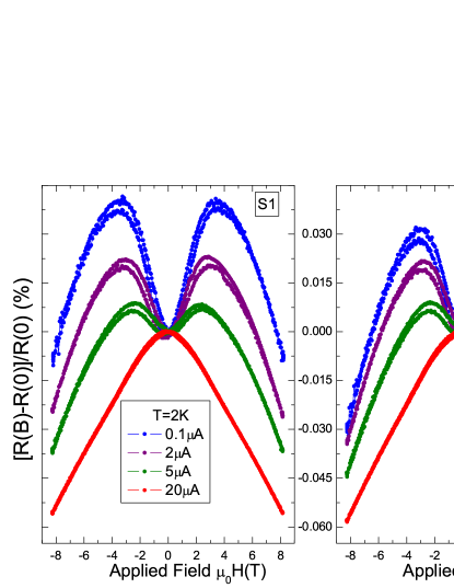
Figure 7: Magnetoresistance of samples S1 and S2 as a function of magnetic field applied normal to the main axis of the CNT bundles at 2 K and at different currents. Note the development of the positive MR the lower the input current as well as the field hysteresis.

At temperatures $T\lesssim 10~{}$K, i.e. in the region where the nonlinear contribution that follows the FIT model (see Fig. 5 and Eq. (6)) appears, an extra positive MR starts to be measurable as can be clearly seen in Fig. 7. There are a few peculiarities about the observed behavior we would like to emphasize:

a) The positive MR is in clear contrast to the ferromagneticlike negative MR behavior observed at higher temperatures, compare Fig. 6 with Fig. 7. This positive and hysteretic (see Fig. 8(b)) MR appears as an additive contribution to the negative one, similar to the addition of the two contributions to the total resistance, see Eq. (5).

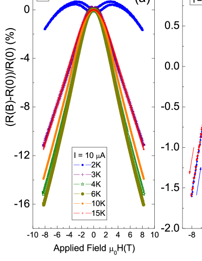
Figure 8: (a) Magnetoresistance of sample S1 as a function of magnetic field applied normal to the main axis of the CNT bundles at different temperatures at fixed current. Note the development of the positive MR the lower the temperature as well as the field hysteresis. (b) The same magnetoresistance data as in (a) but at 2K. The inset shows the temperature dependence of the field $B_{\rm irr}(T)$ defined as the field within the field hysteresis loop at which the hysteresis vanishes. The continuous line follows a simple quadratic $T$-dependence with $B_{\rm irr}(0)=5.9~{}$T and $T_{c}=15~{}$K.

b) The amplitude of the positive MR and the field hysteresis decreases with temperature, see Fig. 8(a). Figure 8(b) shows in more detail the hysteresis loop at 2 K and at an input current of $10~{}\mu$A. As a way to characterize the temperature dependence of the extra contribution to the MR, we define the field $B_{\rm irr}(T)$ at which the hysteresis in the MR vanishes. The temperature dependence of $B_{\rm irr}(T)$ is shown in the inset of Fig. 8(b) and follows roughly a quadratic temperature dependence. This dependence indicates the vanishing of the hysteresis at a critical temperature $T_{c}\simeq 15~{}$K.

c) Figure 9 shows the magnetic hysteresis of sample S1 at $T=2~{}$K after subtraction of the negative MR following Eq. (8), as done at high temperatures. After subtraction, the MR hysteresis loop shows a behavior compatible to superconductors, but also to ferromagnets. The clear addition of the two contributions plus the temperature range where the positive MR and the field hysteresis are observed, indicate a relationship of this phenomenon with the properties of the junctions.

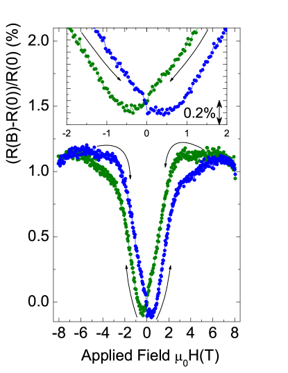
Figure 9: The main panel shows the field hysteresis at $T=2~{}$K and input current $I=0.1~{}\mu$A of sample S1 after subtracting the negative MR contribution following a fit to the high field data using Eq. (8), see Fig. 6. The upper inset blows up the low field region.

d) The behavior of the positive MR as well as of the field hysteresis indicate that the input current plays a mayor role in the development of this phenomenon. For a better characterization of its influence we have measured the change of $B_{\rm irr}$ and the change of the field $B_{m}$ (defined at the minimum of the MR) with current at a fixed temperature. The results are shown in Fig. 10 and indicate a decrease approximately linearly with current of all these two quantities.

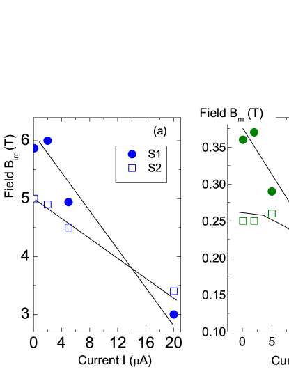
Figure 10: (a) $(\bullet,\square)$: Field at which the field loop gets reversible $B_{\rm irr}$ vs. applied current, for sample S1 and S2, respectively. (b) Field at the minimum of the MR $B_{m}$, see inset in Fig. 9, vs. applied current for samples S1 and S2 at $T=2~{}$K.

The extraordinary hysteresis suggests either the existence of pinning of magnetic entities or a MR hysteresis related to some spin-valve configurations as observed in single-wall CNT with one or two magnetically ordered terminals [37]. Because we do not use any magnetically ordered terminals (in our case those are non-magnetic silver paste) one may think that the magnetically ordered DWCNT themselves, as the negative MR indicates (see Fig. 6), act as spin polarized sources. However, it appears difficult that the DWCNT themselves act simultaneously as ferromagnetic source and drain with different magnetic characteristics to produce the necessary hysteresis. In the case the magnetic entities are magnetic domains existing in the magnetically ordered DWCNT whose walls can be pinned, it appears unlikely that the domain walls can produce such large hysteresis in the MR with a coercive field in the range of $B_{m}(T=2~{}$K$)\simeq 0.35~{}$T at low input currents, see Fig. 10(b). Note that no measurable hysteresis within experimental resolution was measured in the negative MR above 15 K.

There are several hints that suggest that the observed positive MR at low enough currents can be related to a superconducting state, namely: (1) The clear input current dependence, see Fig. 10, indicates that the positive and hysteretic MR should be related to the junctions potential barrier that opens below 15 K. This dependence suggests the existence of a critical Josephson-like current. The Josephson junctions with their two superconducting regions should be localized at certain junctions between DWCNT observed in TEM and SEM measurements.

(2) The value of magnetic field of several Tesla at which the MR saturates, see for example Fig. 12, is of the same order as the upper critical field $H_{c2}$ observed in superconducting coupled $4~{}$Å CNT arrays [38].

(3) The critical temperature $T_{c}\simeq 15~{}$K obtained in our samples coincides with several other $T_{c}$ reported in superconducting $4~{}$Å CNT coupled arrays [38], superconducting $4~{}$Å CNT/Zeolite composites [10], as well as DWCNT arrays [11], and last but not least, in thin graphite flakes with internal interfaces after application of an electric field (with electrical contacts at the top graphene plane) [19].

(4) Finally, we note that the current necessary to depress substantially the positive MR and its hysteresis is $20\ldots 50~{}\mu$A, see Figs. 7 and 10, which is of the same order as the current measured in superconducting coupled $4~{}$Å CNT arrays to reach their normal state [38].

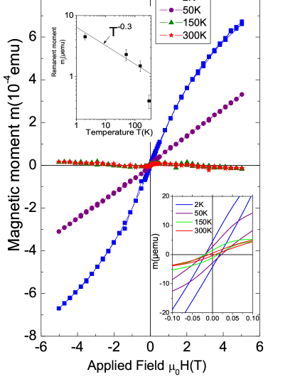
Figure 11: Magnetic field hysteresis for the sample S1 (mass $\sim 1$ mg) measured at different temperatures. Note that due to the used sample holder there is no extra magnetic background signal to be subtracted. The bottom right inset shows the same data expanding the low field region without including the virgin curves for clarity. The top left inset shows the temperature dependence of the remanent moment obtained from the field hysteresis curves.

3.3 Magnetization results

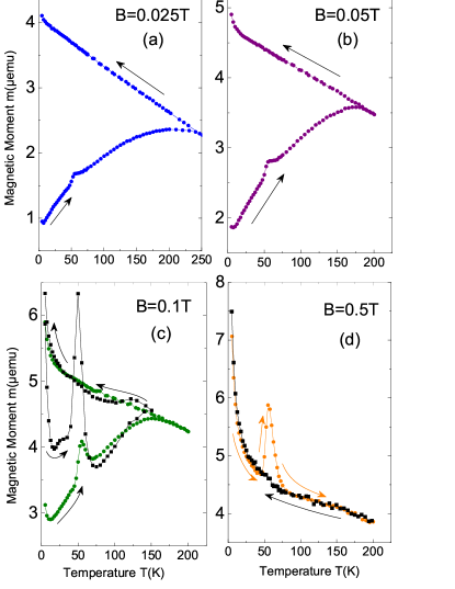
Figure 12: Zero field cooled and field cooled curves (warming up and cooling down respectively), of a DWCNT-bundle of sample S2 of mass $\simeq 1~{}$mg mass, at four different fields applied normal to the main axis of the CNT. Two runs taken at $B=0.1~{}$T and at different maximum temperatures are shown in the corresponding figure as an example of the fair reproducibility of the measurements.

Figure 13: The experimental data points represent the calculated difference between the FC and ZFC curves of sample S1 obtained at $B=0.05~{}$T choosing a maximum temperature of 45 K to avoid the influence of the 50K-peak observed in the ZFC curve. The background difference from the large ferromagnetic contribution has been subtracted using a simple linear in temperature relationship, i.e. (FC-ZFC)${}_{\rm FM}\simeq 2.3\times 10^{-8}(45-T[{\rm K}])-10^{-7}$ [emu].

Taking into account that the magnetotransport properties of the DWCNT bundles reveal one main contribution, a ferromagnetic-like in the whole temperature range, we expect that the magnetization shows a behaviour compatible with it. Figure 11 shows the field hysteresis of the magnetic moment measured in a bundle of DWCNT with the field normal to the main axis of the CNT and at different temperatures. The shown data are as measured, i.e. no subtraction of any background has been done. Note that the used sample holder does not show any extra background. In one of the insets of Fig. 11 we show the same data but in a expanded field scale. One identifies a coercive field of the order of 0.02 T at the lowest temperatures. The magnetization results indicate a paramagnetic and ferromagnetic contributions with a ferromagnetic magnetization that saturates at fields of the order of 0.5 T and remains finite even at room temperature, see inset in Fig. 11. Assuming that the detected Fe-concentration would be ferromagnetic, we expect a maximum magnetic moment at saturation of the order of $m_{\rm Fe,\rm{sat}}\simeq 50~{}\mu$emu. This value is comparable with the saturation magnetic moment of the DWCNT $m_{\rm{sat}}\sim 60~{}\mu$emu at 2 K, estimated after roughly subtracting the large paramagnetic contribution observed in the DWCNT bundle, see Fig. 11. On the other side, the measured paramagnetic contribution clearly overwhelms the largest contribution expected from the Fe impurities by more than a factor of ten. Therefore, the question is, which amount of the ferromagnetic signal does correspond to the DWCNT and which to Fe? Without the knowledge of the magnetic properties of the Fe-containing grains, it is not possible to completely clarify this question because the behavior of the magnetization depends on the stoichiometry (e.g., Fe₃O₄, Fe₃C, etc.) and size of the Fe-containing grains. Comparing the transport and magnetization data related only to the ferromagnetic state, an interesting similarity can be noted. The remanent magnetic moment obtained from the field hysteresis at zero field follows a temperature dependence $T^{-0.3}$ to $\sim 150~{}$K, see upper left inset in Fig. 11. This is the same temperature dependence we would obtain for the ferromagnetic magnetization from the negative magnetoresistance at fixed high fields, see inset in Fig. 6. This similarity suggests that at least part of the ferromagnetic signal in the magnetization measurements might come from the DWCNT themselves.

It should be clear that the possible signal in the magnetization coming from the superconducting-like contribution observed at very low input currents in the MR (see Sec. 3.2.2), is expected to be small and added to the overwhelming para- and ferromagnetic contributions. The measured field hysteresis provides us no clear hints about this extra contribution. Therefore, we decided to measure the temperature hysteresis, i.e. the zero field cooled (ZFC) measured by warming and field cooled (FC) measured afterwards during cooling at fixed applied fields. The results are shown in Fig. 12 at four different fields and at maximum temperatures of 150 K ($B=0.1~{}$T), 200 K ($B=0,05,0.1,0.5~{}$T) and 250 K ($B=0.025~{}$T). The main observation we would like to stress is the large temperature hysteresis that gets smaller the larger the applied field, in agreement with the ferromagnetic field hysteresis loop. This hysteresis in temperature and magnetic field support the existence of magnetic order in our DWCNT, whatever its origin.

In the ZFC, warming up curves a clear maximum at $T\sim 50~{}$K is observed. This maximum, which is a prominent anomaly that shifts slightly to higher temperatures with the applied field, is anomalous because at large enough fields it overwhelms the FC curve. We do not have an explanation for it but we can rule out that it is due to the usual oxygen signal from the SQUID cryostat, since we checked its reproducibility in two SQUIDs and measuring other samples, which do not show any oxygen peak. The reproducibility of this peak indicates that, even if this would be related to oxygen, it should come from the DWCNT bundles. It is interesting to note that a similar behavior has been reported for a superconducting amorphous carbon-sulfur (a-CS) powder in Ref. [39], see also Figs. 14 and 15 in [40], and in the same temperature range. In contrast to those reports, however, the peak in the ZFC curve we observe is always reproducible in the ZFC curves and does not depend on time and/or how many times we measured the ZFC curves. Nevertheless the similarities are remarkable and, as pointed out in Ref. [40], the fact that at the maximum the ZFC curve is above the FC curve, is unique. Even if this maximum would be related to magnetic impurities, the mechanisms that produce such an anomalous behavior remains still unclear.

Due to the large background signal coming from the ferro- and paramagnetic contributions and the large ZFC peak (and its irreversibility) at 50 K, we decided to measure the ZFC-FC curves selecting 45 K as the maximum temperature, applying a relatively small field of 0.05 T. The idea was to check whether a superconducting-like difference in the temperature hysteresis is observed below 15 K. Figure 13 shows the obtained difference between FC and ZFC curves at 0.05 T and after subtraction of a linear in temperature background contribution. The obtained difference starts to increase below $\simeq 15~{}$K, in agreement with the results shown in Fig. 8. We note that this difference is much smaller than the difference from the ferromagnetic contribution and the absolute value of the total magnetic signal. Because the hysteresis in the MR is observed up to large fields, see Fig. 9, one would expect to see it in the ZFC-FC runs as well. However, the paramagnetic contribution is several orders of magnitude larger than the expected hysteresis and, therefore and within SQUID resolution, no clear superconducting-like hysteresis response could be obtained.

4 Conclusion and open issues

Measurements of the magnetotransport properties of bundles of DWCNT reveal the existence of magnetic order that remains up to room temperature. At small enough input currents, a positive and hysteretic magnetoresistance behaviour is observed that vanishes at $T\simeq 15~{}$K, compatible with the existence of superconductivity, in agreement with different reports of CNT as well as in other carbon-based materials that show a similar superconducting transition temperature. Although not a straightforward proof due to the complexity of the observed hysteresis and the possible contribution of Fe impurities, we may conclude that the magnetization data appear compatible to some extent to the interpretation of the magnetotransport data.

Several questions remain unanswered yet. The first is related to the observed magnetic order. Is it due to defects, like C-vacancies or to the curvature of the CNT, or hydrogen? Taking into account the evidence obtained for graphite and theoretical works, all those possibilities may apply. Future experiments should try to decrease substantially the amount of Fe impurities as well as to measure an isolated DWCNT to study the change in the magnetotransport properties with annealing and/or proton bombardment, for example. Second, where is the superconductivity actually localized and why is it triggered there? Which kind of magnetic vortices exist that produce such relatively large hysteresis in the MR? Due to the apparent relationship of this transition to the development of a tunneling region, it is tempting to assume that the superconductivity appears at the junctions of the DWCNT. We note that a junction may consist of a region of two bilayers graphene, twisted by a certain angle. In this case, regions with flat bands may appear where superconductivity develops, following recently published work on the extraordinary superconducting properties of graphite interfaces, see [41, 42] and refs. therein. Those localized regions are expected to be rather small, below 1 $\mu$m in length, see Figs. 1 and 2. If superconductivity is localized at these 2D interfaces, can an applied field produce the so-called Pearl vortices [43], in such a small junction area? We note that these vortices have the property to have a giant effective penetration depth $\Lambda\simeq\lambda^{2}/d$, where $\lambda$ is the London penetration depth and $d$ is the thickness of the superconducting layer. As argued in the original publication [43], it means that they have a very long range interaction. In this case the bundle of Pearl vortices may be pinned by the existence of pinning centers distributed in a much larger region than the superconducting region itself, providing such a relatively large MR hysteresis.

The work in Israel was partially supported by the Israel National Research Center for Electrochemical Propulsion (INREP; I-CORE Program of the Planning and Budgeting Committee and The Israel Science Foundation 2797/11). Fruitful discussions with Prof. Y. Yeshurun from Bar Ilan University are gratefully acknowledged.

References

- [1] O. V. Yazyev, Emergence of magnetism in graphene materials and nanostructures, Rep. Prog. Phys. 73 (2010) 056501.
- [2] P. Esquinazi, W. Hergert, D. Spemann, A. Setzer, A. Ernst, Defect-induced magnetism in solids, Magnetics, IEEE Transactions on 49 (8) (2013) 4668–4674.
- [3] Y. Ma, P. O. Lehtinen, A. S. Foster, R. M. Nieminen, Magnetic properties of vacancies in graphene and single-walled carbon nanotubes, New Journal of Physics 6 (2004) 68–1–15.
- [4] Y. Ma, P. O. Lehtinen, A. S. Foster, R. M. Nieminen, Hydrogen-induced magnetism in carbon nanotubes, Phys. Rev. B 72 (2005) 085451–1–6.
- [5] T. Saito, T. Ozeki, K. Terashima, Hydrogen-induced magnetism in carbon nanotubes, Solid State Commun. 136 (2005) 546–549.
- [6] A. L. Friedman, H. Chun, Y. J. Jung, D. Heiman, E. R. Glaser, L. Menon, Possible room-temperature ferromagnetism in hydrogenated carbon nanotubes, Phys. Rev. B 81 (2010) 115461. doi:10.1103/PhysRevB.81.115461.
- [7] A. L. Friedman, H. Chun, D. Heiman, Y. J. Jung, L. Menon, Investigation of electrical transport in hydrogenated multiwalled carbon nanotubes, Physica B: Condensed Matter 406 (4) (2011) 841 – 845.
- [8] Z. K. Tang, L. Zhang, N. Wang, X. X. Zhang, G. H. Wen, G. D. Li, J. N. Wang, C. T. Chan, P. Sheng, Superconductivity in 4 angstrom single-walled carbon nanotubes, Science 292 (5526) (2001) 2462–2465.
- [9] M. Kociak, A. Y. Kasumov, S. Guéron, B. Reulet, I. I. Khodos, Y. B. Gorbatov, V. T. Volkov, L. Vaccarini, H. Bouchiat, Superconductivity in ropes of single-walled carbon nanotubes, Phys. Rev. Lett. 86 (2001) 2416–2419.
- [10] R. Lortz, Q. Zhang, W. Shi, J. T. Ye, C. Qiu, Z. Wang, H. He, P. Sheng, T. Qian, Z. Tang, N. Wang, X. Zhang, J. Wang, C. T. Chan, Superconducting characteristics of 4-carbon nanotube/zeolite composite, Proceedings of the National Academy of Sciences 106 (18) (2009) 7299–7303.
- [11] W. Shi, Z. Wang, Q. Zhang, Y. Zheng, C. Ieong, M. He, R. Lortz, Y. Cai, N. Wang, T. Zhang, H. Zhang, Z. Tang, P. Sheng, H. Muramatsu, Y. A. Kim, M. Endo, P. T. Araujo, M. S. Dresselhaus, Superconductivity in bundles of double-wall carbon nanotubes, Sci. Rep. 2 (2012) 625.
- [12] I. Takesue, J. Haruyama, N. Kobayashi, S. Chiashi, S. Maruyama, T. Sugai, H. Shinohara, Superconductivity in entirely end-bonded multiwalled carbon nanotubes, Phys. Rev. Lett. 96 (2006) 057001.
- [13] N. Murata, J. Haruyama, Y. Ueda, M. Matsudaira, H. Karino, Y. Yagi, E. Einarsson, S. Chiashi, S. Maruyama, T. Sugai, N. Kishi, H. Shinohara, Meissner effect in honeycomb arrays of multiwalled carbon nanotubes, Phys. Rev. B 76 (2007) 245424.
- [14] M. Ferrier, F. Ladieu, M. Ocio, B. Sacépé, T. Vaugien, V. Pichot, P. Launois, H. Bouchiat, Superconducting diamagnetic fluctuations in ropes of carbon nanotubes, Phys. Rev. B 73 (2006) 094520.
- [15] Y. Yang, G. Fedorov, J. Zhang, A. Tselev, S. Shafranjuk, P. Barbara, The search for superconductivity at van hove singularities in carbon nanotubes, Supercond. Sci. Technol. 25 (2012) 124005.
- [16] S. Belluci, M. Cini, P. Onorato, E. Perfetto, Suppression of electron-electron repulsion and superconductivity in ultra-small carbon nanotubes, J. Phys.: Condens. Matter 18 (2006) S2115–S2126.
- [17] J. Noffsinger, M. L. Cohen, Electron-phonon coupling and superconductivity in double-walled carbon nanotubes, Phys. Rev. B 83 (2011) 165420.
- [18] M. Khalid, P. Esquinazi, Hydrogen-induced ferromagnetism in ZnO single crystals investigated by magnetotransport, Phys. Rev. B 85 (2012) 134424.
- [19] A. Ballestar, P. Esquinazi, J. Barzola-Quiquia, S. Dusari, F. Bern, R. da Silva, Y. Kopelevich, Possible superconductivity in multi-layer-graphene by application of a gate voltage, Carbon 72 (2014) 312–320.
- [20] G. D. Nessim, M. Seita, K. P. O’Brien, A. J. Hart, R. K. Bonaparte, R. R. Mitchell, C. V. Thompson, Low temperature synthesis of vertically aligned carbon nanotubes with ohmic contact to metallic substrates enabled by thermal decomposition of the carbon feedstock, Nano Letters 9 (2009) 3398–3405.
- [21] G. D. Nessim, A. Al-Obeidi, H. Grisaru, E. S. Polsen, C. Ryan Oliver, T. Zimrin, A. John Hart, D. Aurbach, C. V. Thompson, Synthesis of tall carpets of vertically aligned carbon nanotubes by in situ generation of water vapor through preheating of added oxygen, Carbon 50 (2012) 4002–4009.
- [22] D. Spemann, P. Esquinazi, A. Setzer, W. Böhlmann, Trace element content and magnetic properties of commercial HOPG samples studied by ion beam microscopy and squid magnetometry, AIP Advances 4 (2014) 107142.
- [23] A. G. Souza Filho, A. Jorio, G. Dresselhaus, M. S. Dresselhaus, R. Saito, A. K. Swan, M. S. Ünlü, B. B. Goldberg, J. H. Hafner, C. M. Lieber, M. A. Pimenta, Effect of quantized electronic states on the dispersive raman features in individual single-wall carbon nanotubes, Phys. Rev. B 65 (2001) 035404.
- [24] J. Barzola-Quiquia, P. Esquinazi, M. Rothermel, D. Spemann, T. Butz, Proton-induced magnetic order in carbon: Squid measurements, Nuclear Instruments and Methods in Physics Research B 256 (2007) 412–418.
- [25] A. L. Efros, B. I. Shklovskii, Coulomb gap and low temperature conductivity of disordered systems, J. Phys. C: Solid State Phys. 8 (4) (1975) L49.
- [26] P. Sheng, E. K. Sichel, J. I. Gittleman, Fluctuation-induced tunneling conduction in carbon-polyvinylchloride composites, Phys. Rev. Lett. 40 (1978) 1197–1200.
- [27] P. Sheng, Fluctuation-induced tunneling conduction in disordered materials, Phys. Rev. B 21 (1980) 2180–2195.
- [28] M. S. Fuhrer, J. Nygard, L. Shih, M. Forero, Y.-G. Yoon, M. S. C. Mazzoni, H. J. Choi, J. Ihm, S. G. Louie, A. Zettl, P. L. McEuen, Crossed nanotube junctions, Science 28 (2000) 494.
- [29] M. Bockrath, D. H. Cobden, P. L. McEuen, N. G. Chopra, A. Zettl, A. Thess, R. E. Smalley, Single-electron transport in ropes of carbon nanotubes, Science 275 (5308) (1997) 1922–1925.
- [30] G. Kim, S. Jhang, J. Park, Y. Park, S. Roth, Non-ohmic current voltage characteristics in single-wall carbon nanotube network, Synthetic Metals 117 (2001) 123 – 126.
- [31] Y.-R. Lai, K.-F. Yu, Y.-H. Lin, J.-C. Wu, J.-J. Lin, Observation of fluctuation-induced tunneling conduction in micrometer-sized tunnel junctions, AIP Advances 2.
- [32] R. Khosla, J. Fischer, Magnetoresistance in degenerate cds: Localized magnetic moments, Phys. Rev. B 2 (1970) 4084–4097.
- [33] O. Volnianska, P. Boguslawski, Magnetism of solids resulting from spin polarization of orbitals, J. Phys.: Condens. Matter 22 (2010) 073202.
- [34] J. Barzola-Quiquia, P. Esquinazi, M. Rothermel, D. Spemann, T. Butz, N. García, Experimental evidence for two-dimensional magnetic order in proton bombarded graphite, Phys. Rev. B 76 (2007) 161403(R).
- [35] M. A. Ramos, J. Barzola-Quiquia, P. Esquinazi, A. Muñoz Martin, A. Climent-Font, M. García-Hernández, Magnetic properties of graphite irradiated with MeV ions, Phys. Rev. B 81 (2010) 214404.
- [36] J. Barzola-Quiquia, N. Klingner, J. Krüger, A. Molle, P. Esquinazi, A. Leonhardt, M. T. Martínez, Quantum oscillations and ferromagnetic hysteresis observed in iron filled multiwall carbon nanotubes, Nanotechnology 23 (2012) 015707.
- [37] A. Jensen, J. R. Hauptmann, J. Nygård, P. E. Lindelof, Magnetoresistance in ferromagnetically contacted single-wall carbon nanotubes, Phys. Rev. B 72 (2005) 035419.
- [38] Z. Wang, W. Shi, H. Xie, T. Zhang, N. Wang, Z. Tang, X. Zhang, R. Lortz, P. Sheng, I. Sheikin, A. Demuer, Superconducting resistive transition in coupled arrays of carbon nanotubes, Phys. Rev. B 81 (2010) 174530.
- [39] I. Felner, E. Prilutskiy, J Supercond Nov Magn 25 (2012) 2547.
- [40] I. Felner, Superconductivity and unusual magnetic behavior in amorphous carbon, Materials Research Express 1 (2014) 016001.
- [41] A. Ballestar, J. Barzola-Quiquia, T. Scheike, P. Esquinazi, Evidence of Josephson-coupled superconducting regions at the interfaces of highly oriented pyrolytic graphite, New J. Phys. 15 (2013) 023024.
- [42] P. Esquinazi, T. T. Heikkilä, Y. V. Lysogoskiy, D. A. Tayurskii, G. E. Volovik, On the superconductivity of graphite interfaces, JETP Letters 100 (2014) 336–339, arXiv:1407.1060.
- [43] J. Pearl, Current distribution in superconducting films carrying quantized fluxoids, Applied Physics Letters 5 (1964) 65–66.