A many–body perturbation theory approach to the electron–phonon interaction with density–functional theory as a starting point
Andrea Marini
Istituto di Struttura della Materia of the National Research Council, Via Salaria Km 29.3,
I-00016 Monterotondo Stazione, Italy
European Theoretical Spectroscopy Facilities (ETSF)
S. Poncé
Université catholique de Louvain, Institute of Condensed Matter and Nanosciences,
NAPS Chemin des étoiles 8, bte L07.03.01, B-1348 Louvain-la-neuve, Belgium
European Theoretical Spectroscopy Facilities (ETSF)
X. Gonze
Université catholique de Louvain, Institute of Condensed Matter and Nanosciences,
NAPS Chemin des étoiles 8, bte L07.03.01, B-1348 Louvain-la-neuve, Belgium
European Theoretical Spectroscopy Facilities (ETSF)
Abstract
The electron–phonon interaction plays a crucial role in many fields of physics and chemistry. Nevertheless, its actual
calculation by means of modern many–body perturbation theory is weakened by the use of model Hamiltonians that
are based on parameters difficult to extract from the experiments.
Such shortcoming can be bypassed by using density–functional theory to evaluate the electron–phonon scattering amplitudes, phonon frequencies and electronic
bare energies.
In this work, we discuss how a consistent many–body diagrammatic
expansion can be constructed on top of density–functional theory.
In that context, the role played by screening and self–consistency when all the components of the electron–nucleus and nucleus–nucleus interactions are taken into account is paramount.
A way to avoid overscreening is notably presented.
Finally, we derive cancellations rules as well as internal consistency constraints in order to draw a clear, sound and practical scheme to merge
many–body perturbation and density–functional theory.
pacs:
71.38.-k,71.15.Mb, 71.15.-m
In physics and chemistry the interaction between electronic and vibrational
degrees of freedom is at the origin of a multitude of phenomena. Focusing on
solid state physics, this coupling usually determines the electrical
and thermal conductivity of metals as well as carrier lifetime in
doped semiconductorsZiman (1960). It also induces the transition to a
superconducting phase in many solids and nanostructuresMitsuhashi et al. (2010).
The electron–nucleus coupling also plays a role in the renormalization of electronic
bandsAllen and Cardona (1983), carriers mobility in organic devicesGosar and Choi (1966) and
dissociation at the donor/acceptor interface in organic
photovoltaicTamura et al. (2008).
This coupling can naturally interact with other couplings like the magnetic field leading, for example, to the spin-Seebeck effectAdachi et al. (2013).
This effect is nowadays the subject of an intense research activity for its crucial role in new emerging fields of
experimental and theoretical physics. The electron–nucleus coupling plays a crucial role in the relaxation and dissipation of
photo–excited carriers in
pump and probe experiments Bernardi et al. (2014); Sangalli and Marini (2014). Similarly, modern
Angle–Resolved Photoemission Spectra (ARPES) experiments have recently disclosed the complex and temperature dependent structures appearing in the spectral functions of
several oxidesMoser et al. (2013). These structures quite remarkably resemble similar structures predicted to exist in conjugated polymersCannuccia and Marini (2011a, 2012)
pointing to a strong effect whose physical origin is still not completely clear.
From the theoretical point of view, the most up–to–date scheme to calculate and predict the ground– and excited–state properties of
a wide range of materials is based on the merging of
Density–Functional–Theory (DFT)R.M.Dreizler and E.K.U.Gross (1990) with Many–Body Perturbation
Theory (MBPT)Onida et al. (2002).
DFT is a broadly used ab-initio ground–state theory,
that allows to calculate exactly electronic density and total energy without adjustable parameter.
The merging of DFT with perturbation theory gives the so-called
Density-Functional Perturbation TheoryBaroni et al. (1987); Gonze (1997); Baroni et al. (2001) (DFPT). The DFPT is a powerful computational tool for the direct treatment of phonons.
However, the DFT computation of excited electronic states
properties like the bandgap energies is a known problematic topic R.M.Dreizler and E.K.U.Gross (1990).
As a result, MBPT
is nowadays the preferred alternative to DFT for that purpose. It
is based on the accurate treatment of correlation effects by means of the
Green’s function formalism. MBPT is formally correct and leads to a close
agreement with experimentvan Schilfgaarde et al. (2006) but is extremely
computationally demanding. A natural way to solve this issue is to merge the
quick DFT calculation with the accurate MBPT one. The latter method
is often referred to as ab-initio Many-Body Perturbation
Theory Onida et al. (2002) (ai–MBPT).
In this method, DFT provides a suitable single–particle basis for the MBPT scheme.
This methods has been applied successfully to correct the well–known band–gap underestimation problem of
DFTGrüning et al. (2006); Niquet and Gonze (2004).
Although the ai–MBPT aims at calculating the excited state properties with an unprecedent precision,
it is commonly applied by neglecting the effect of lattice vibrations.
Even today, most of the ai–MBPT results are compared with finite-temperature experimental dataCardona et al. (1999).
Such comparison is not even well motivated at zero temperature as the lattice vibrations induce a zero–point motion effect
that can be sizeable Cannuccia and Marini (2011a, 2012); Gonze et al. (2011); Giustino et al. (2010),
e.g. on the order of 0.4–0.6 eV for the direct and indirect band gaps of diamond Poncé et al. (2014a); Antonius et al. (2014).
This represent a clear motivation to develop a coherent ab–initio theory in which the electron–phonon interaction is rigorously included on top
of ai–MBPT.
The need for such theory is exemplified by the very fragmented historical development of the ab–initio approach to the temperature dependence
of the electronic structure due to the electron–phonon interaction.
From the fifties to the late eighties, a coherent ab–initio framework was still not devised and the electron–phonon interaction
was initially investigated and computed in a semi-empirical context
by FanFan (1950, 1951). His theory had no adjustable parameters and was based on the first-order perturbed
Hamiltonian. During the same period, AntoncíkAntoncík (1955), followed by othersKeffer et al. (1968); Walter et al. (1970); Kasowski (1973), developed empirical Debye-Waller (DW) corrections to the nuclear potential.
Only in 1976, Allen and HeineAllen and Heine (1976) rigorously unified the Fan and DW corrections in a common framework. Their approach, combined with the use of a semi-empirical
model, allows for a re-writing of the problem in terms of first-order derivatives of an effective potential only. Calculations of the
electron–phonon renormalization effects were then led by Cardona and
coworkersAllen and Cardona (1981, 1983); Lautenschlager et al. (1985); Zollner et al. (1992), including Allen.
The resulting approach is now called the Allen-Heine-Cardona (AHC) theory.
In 1989, the first ab–initio calculation of the temperature dependence of the gap was attempted, by King-Smith et alKing-Smith et al.(1989), based on DFPT.
Starting from there, several
first–principle calculations have been done, relying mainly on three types of formalisms: (i) time averaging of bandgap obtained using first principles molecular dynamics
simulationsFranceschetti (2007); Kamisaka et al. (2008); Ibrahim et al. (2008); Ramírez et al. (2006, 2008); (ii) frozen phonons (FP) calculations Monserrat et al. (2013); Antonius et al. (2014); Capaz et al. (2005); Patrick and Giustino (2013); Han and Bester (2013); Poncé et al. (2014b) and
(iii) the AHC approach implemented in a full ab–initio framework by using DFT and DFPT as a reference system Giustino et al. (2010); Poncé et al. (2014a); Antonius et al. (2014); Poncé et al. (2014b); Kawai et al. (2014).
All these approaches are based on an adiabatic and static treatment of the electron–phonon interaction. This limitation was overcome by using
the dynamical version of MBPT by Marini et alMarini (2008); Cannuccia and Marini (2011a, 2012) who focused on retardation effects.
Since then, there have been an increasing number of studies in which the electron–phonon interaction is fully included
in the computation of the electronic structure, well beyond DFT. Still, several basic questions remain. In particular,
the use of an electron–phonon interaction whose strength is computed from DFT, in a formalism that goes beyond DFT, e.g. the ai–MBPT approach, leads to
several ambiguities due to the simultaneous inclusion of different levels of correlation at the MBPT and DFT/DFPT level.
Indeed, the DFPT electron–phonon interaction is naturally screened as it is computed from the derivative of the self–consistent Kohn-Sham potential with respect to atomic displacements.
This screening is taken as it is in the MBPT part of the ai–MBPT scheme, although it is well known that the diagrammatic technique also predicts the screening of
the electron–phonon interaction consistently with the kind of correlation included in the self–energy Mattuck (1976); Fetter and Walecka (1971).
It has in fact been shown that the size of the zero-point motion renormalization is significantly larger in the MBPT than in the DFPT approachesAntonius et al. (2014).
Another important issue of the ai–MBPT approach is the lack of a diagrammatic interpretation of the screening of the Debye–Waller term. This screening arises quite naturally
in the DFPT Poncé et al. (2014b) and AHC approaches Allen and Heine (1976). It is easy to show that it comes from the DFT self–consistent screened ionic potential. Instead, in the pure MBPT treatment
of electrons and nuclei, this diagram is un–screened.
The Debye–Waller diagram is however usually taken as screened without justification in most practical application because of the DFPT basis.
In addition, a non–rigid nuclei correction to the Debye–Waller contribution Poncé et al. (2014b) is predicted to exist within the DFPT approach. However, this term is notably absent from the standard derivation of the electron–phonon theory based on the MBPT.
The last issue is even more fundamental. Most of the electron–phonon interaction treatments that appears in textbooks, see e.g. Refs. [Mahan, 1998; Fetter and Walecka, 1971; Mattuck, 1976], are based on the study of the homogeneous electronic gas (jellium). At variance with any realistic
material, the jellium model is based on a drastic approximation:
the ions are replaced by a jelly of positive charge, in contrast with realistic materials where the nuclei and their mutual interaction must be taken explicitly into account. This is correctly done in DFT and DFPT but not in the MBPT approach derived from the jellium model.
This paper aims at answering all these questions by devising a coherent, formal and accurate approach to merge the MBPT scheme with DFT and DFPT.
We present a consistent electron–phonon interaction theory based on the MBPT formalism, insisting specifically on the connection between the MBPT and AHC approaches. This work is inspired by the seminal works of
AllenAllen (1978) and van Leeuwenvan Leeuwen (2004), going further by including the full description of the atomic potential into account.
The merging procedure will lead to the natural definition of a series of practical rules and advices about how to perform electron–phonon calculations on top of DFT without
double counting problems. These series of rules are well justified within the ai–MBPT scheme that, in its practical form used in material science calculations,
can be seen as a collection of prescriptions only partially based on a solid theoretical ground and rather inspired by the succesfull comparison with the experiments
of several different materials. This a posteriori validation represents and important part of the ai–MBPT approach.
The structure of the paper is as follows. Section I presents the total Hamiltonian and introduces the notation. In section II, we draw a parallel
between the electron–electron and the electron–phonon self–energies to show what is the source of the problems that arise in the
merging of MBPT with DFT and DFPT. Section III properly defines the reference Hamiltonian to be used as a zero–th order in the many–body expansion.
In Section IV, the different interaction terms are described, including the contributions from the nuclei–nuclei interaction. In
Section V, we perform the formal diagrammatic summations at different level of approximations: Hartree, Hartree–Fock and .
We use the different levels of correlation of these self–energies to discuss
the different role played by self–consistency diagrams and how the screening of the interaction terms arises.
At the same time we derive cancellation rules that highlight the crucial role
played by the nuclei–nuclei interaction.
Finally, Section VI reviews the DFPT approach to the electron–phonon coupling in order, in Section VII, to compare the different properties of the DFT and of the Many–Body approach.
We provide, in a practical and schematic way, a series of formal properties of the Many–Body expansion performed on top of the DFT reference Hamiltonian. We discuss, from a diagrammatic perspective, the
physical origin of the Debye–Waller terms beyond the screened rigid–ion contribution (Section VII.3) and a practical approach to calculate iteratively the n–th order derivatives of the DFT self–consistent potential
(Section VII.4 and Appendix B). Atomic (Hartree) units are used throughout the article.
I The total Hamiltonian
We start from the generic form of the total Hamiltonian of the system, that we divide in its electronic ,
nuclear and electron–nucleus (e–n) contributions,
(1)
where is a generic notation that represents a dependence on the positions of the nuclei.
The electronic and nuclear parts are divided in a kinetic and interaction part
:
(2)
(3)
Note that the nuclear kinetic energy depends on the nuclear momenta, and not on the actual positions of the nuclei.
In the above definitions, the operators are bare (un–dressed). The analysis of the dressing of that arises as a consequence of the electronic correlations is one of the key objective of this work.
Indeed, in the Many–Body (MB) approach, this dressing appears in the perturbative expansion in the form of electron–hole pair excitations and therefore, cannot be introduced a priori
in the definition of the Hamiltonian.
The explicit expression for the bare (e–n) interaction term is
(4)
where is the nuclear position operator for the nucleus
inside the cell (the cell is located at position ), is the corresponding charge, is the electronic position operator of the electron and
is the
bare Coulomb potential. Similarly,
(5)
(6)
with .
We now use the notation , or equivalently , to indicate a quantity or an operator that is evaluated
with the nuclei frozen in their equilibrium crystallographic positions (). We expand the Hamiltonian as a Taylor series up to second order in the
nuclear displacements,
(7)
where and are Cartesian coordinates and
(8)
The equilibrium crystallographic positions are defined, in the present context, as the
positions minimizing the expectation energy of the Born-Oppenheimer Hamiltonian (with fully correlated electrons), i.e. all the contributions
to the total Hamiltonian, except the nuclear kinetic energy,
(9)
Those positions are equivalently defined by the condition that
the expectation of the Born-Oppenheimer force acting on the nucleus located at position is zero
(10)
The average in Eq. (10) is done on the exact electronic ground state of the Born-Oppenheimer Hamiltonian. Still, the present theory
will go beyond the Born-Oppenheimer approximation by considering fluctuations around the equilibrium positions.
II The problem
The problem we aim at solving is how to treat the effect of the two last terms in the right–hand side of Eq. (7) and how to do it
by merging the MB approach, well-established for the treatment of , with a DFT description of the reference electronic and nuclear systems.
When the Hamiltonian represents indeed
a purely electronic problem, for which the MB approach is well-established in the
literatureOnida et al. (2002); Mahan (1998); Hedin and Lundqvist (1970); Fetter and Walecka (1971). It relies on the definition of an electronic self–energy
that is a complex and non–local function in frequency and space. can be approximated by following different strategies available
in the literature (like the well–known approximation Aryasetiawan and Gunnarsson (1998)).
For periodic solids, once the self–energy is known, the calculation of the correction to an energy level can be obtained by solving the corresponding
Dyson equation ( is a band index and the corresponding wavevector).
Usually, the MB methodology starts from an independent–particle (IP) electronic Hamiltonian that includes only the kinetic
electronic operator and the electron-nucleus operator,
(11)
The analysis of the correlated electronic Hamiltonian,
(12)
is addressed through the diagrammatic expansion.
A simple approximation to the solution of the Dyson Equation that fully captures the role played by correlation effects
is the
on–the–mass–shell approximation
where:
(13)
where and are the n–th single–particle eigenstate
and eigenenergy of the independent–particle (IP) Hamiltonian .
In the present context, where we must consider different configurations of nuclei, and determine
also the equilibrium geometry through Eq. (10), the initial correlation present in the reference system for the diagrammatic expansion must be carefully analyzed.
Adding the nucleus-nucleus energy to gives
(14)
namely, the Born-Oppenheimer Hamiltonian without electron–electron interaction operator .
This initial Hamiltonian do not include electron–electron correlations, and can be used as the starting point of a MB approach to the electronic problem.
However, using this Hamiltonian instead of the true Born-Oppenheimer Hamiltonian
means that no electronic correlation energy contribution
appears in the total energy and in the definition of the equilibrium nuclear positions through Eq. (10). This would lead
to a completely irrealistic description of the starting nuclear geometry and vibrational frequencies. Indeed, e.g. the latter could be imaginary,
and this would lead to unusual technical problems with the canonical transformation from the displacement operator to the
phonon creation and annihilation operators.
Thus, the extension of the electronic–only MB approach to the case where nuclear displacements are considered cannot use such a starting point.
As DFT provides a treatment of energy and forces that include the electron–electron interaction, it yields a better starting point than Eq. (14).
DFT is an exact mean–field theory in the sense that
all electronic correlation effects are embodied in a mean–field exchange–correlation (xc) potential which replaces the full electron–electron interaction operator , and depends on the ground-state density . The bracket in denotes a functional dependence.
By adding to the Hartree potential,
, we get the total DFT potential:
(15)
with
(16)
DFT is exact in the sense that the corresponding Kohn–Sham (KS) Hamiltonian
(17)
provides, when the nuclear positions are given, a set of electronic eigenvectors whose corresponding density is the exact ground state density
of (Hohenberg–Kohn theoremR.M.Dreizler and E.K.U.Gross (1990)).
The Hohenberg–Kohn theorem also states that and the ground–state energy are functional of the exact
electronic density .
It follows that, once the correct exchange-correlation functional is used,
DFT gives the exact equilibrium nuclear positions through Eq. (10).
In practice, an exact expression for is not known and
several approximations for it have been proposed in the literature R.M.Dreizler and E.K.U.Gross (1990).
In any case, even the simple local–density approximation (LDA) Ceperley and Alder (1980); Perdew and Zunger (1981), provides quite reasonable structural properties. Thus DFT represents a concrete and accurate
reference Hamiltonian to be used as zero–th order for a diagrammatic expansion that will allow vibrational degrees of freedom to be included.
Formally, at the equilibrium geometry, one decomposes the correlated Hamiltonian as
(18)
At this point, the perturbative expansion is performed in terms of instead of . This is the theoretical basis of the
standard ai–MBPT schemeOnida et al. (2002).
If DFT is used as a reference non–interacting system Eq. (13) does not hold anymore. Its extension can be shown to be
(19)
where is the n–th single–particle eigenstate of with energy .
Note that in Eq. (19) only the and terms appears as the Hartree terms in and cancels out.
Eq. (19) reveals the simplicity of the ai–MBPT scheme. The accuracy
and universality of DFT avoids the use of ad–hoc parameters and the prize to pay (at least in the electronic case) is to simply subtract from the self–energy
the xc potential. This simplicity represents one of the key reasons for the wide–spread use of ai–MBPT .
At this point, one would be tempted to follow the same strategy
in the electron–phonon case by adding to Eq. (18), the nuclear Hamiltonian, , and the contributions from that are linear and quadratic in the atomic displacements.
This is, however, formally not correct. Indeed, when the nuclei are allowed to be displaced from their equilibrium configuration, the DFT (or more directly, DFPT)
will be expanded in a Taylor series,
(20)
with, however,
(21)
This is due to the fact that, in , the electron-phonon interaction terms are statically screened by the electronic dielectric function
while in the Taylor expansion Eq. (7) they are bare, unscreened. In other words,
the ground state density present in Eq. (17) actually depends implicitly on the nuclear coordinates.
In practice, this means that the effect of does not appear only as an additive term in the Dyson equation but it
screens the interaction potentials and .
An additional problem, partially connected to the potential double counting of correlation when DFT is used as the reference Hamiltonian, is due to the fact that
most of the electron-phonon theory has been devised in the jellium model where the nuclei appear only as static and frozen positive charges.
As a consequence, strong approximations on the perturbative expansion are used in textbooks.
This is inconsistent with the microscopic description of the nuclear lattice and indeed represents the most critical shortcoming of the commonly applied
approaches. In all the aforementioned applications of the ai–MBPT schemes (AHC and beyond) is neglected and is screened by hand directly in the initial Hamiltonian.
From these simple arguments we can argue that, although ai–MBPT is a well-established schemeOnida et al. (2002), its extension to the electron-phonon problem is still far from being formally defined.
We would like to apply the MBPT technique to the perturbative expansion of Eq. (7) where the non–interacting Kohn–Sham Hamiltonian and its derivatives as calculated by DFT and DFPT are used.
We propose to apply the standard diagrammatic MBPT on the total bare Hamiltonian, given by Eqs. (7),
explicitly taking into account all interaction terms. We will then examine the properties of the operator in order to
draw a clear and formal comparison between ai–MBPT and DFPT.
In this way, we aim at creating a consistent framework where
the role played by screening and self–consistency is clearly evidenced even when all the components of the electron–nucleus and nucleus–nucleus interactions are taken into account.
III The reference, independent–particle Hamiltonian
As it emerges from the discussion of the previous section, the choice of the non–interacting Hamiltonian to be used as a reference for the perturbative expansion represents the
connection with DFT and thus provides the ab–initio basis for the entire theoretical derivation. This is particularly important for the definition of the phonon modes.
Therefore, we start by introducing a splitting of the total Hamiltonian in an independent particle part
(for independent electrons as well as independent phonons) plus interaction terms,
(22)
Eq.(22) is more suited than Eq. (7) to the MB treatment.
The reference independent–particle Hamiltonian is
(23)
where and are evaluated
at the equilibrium geometry.
We have introduced a reference nucleus–nucleus interaction , a second–order contribution
within the Taylor expansion in the nuclear displacements, that provides the reference phonon modes to be used in the diagrammatic expansion.
This can be defined from DFPT
(24)
with the Born–Oppenheimer total energy of the system calculated within DFT. By construction, the phonon frequencies
and eigenvectors will be equal to those of the Born-Oppenheimer approximation based on the correlated electronic Hamiltonian.
Therefore, Eq. (23) defines an independent–particle Hamiltonian beyond the equilibrium geometry.
The remaining interaction part, up to second order in nuclear displacements, is
(25)
where
(26)
and
(27)
At this point we can introduce the eigenstates of the nuclear harmonic oscillations of , written in terms of
the canonical transformation
(28)
where is a generic DFPT phonon mode with momentum , energy branch
and energy .
is the number of –points in the whole Brillouin Zone (BZ). We assume the –point grid to be uniform so that
we have also –points for the single particle representation.
is the nuclear mass,
is the polarization vector of the atom in the unit cell in the Cartesian direction ,
while and , respectively, are the annihilation and creation operators
of the phonon mode , respectively.
We now introduce a second quantization formulation for the electrons.
If is the electronic eigen–function, we introduce the field operator
(29)
with
(30)
with the annihilation operator of an electron.
By using field operators, the independent-particle Hamiltonian can be written in a second quantization form:
(31)
where the first term corresponds to and the second one to
. The Born-Oppenheimer energy of the ground state at equilibrium geometry
has been redefined to be the zero of energy
(hence e.g. disappears from this expression).
The introduction of a reference nucleus–nucleus potential in was the crucial step to be able to map it with its second quantization form.
Indeed it is well known that phonon dynamics is actually decoupled from the electronic one, as shown in many referencesvan Leeuwen (2004); Mattuck (1976).
Nonetheless, the phonon dynamics can describe accurately the vibrational properties of a real system only if it feels the electronic screening. Such screening is accounted for in DFPT by the reference potential operator.
IV The electron–phonon interaction terms
Thanks to the definition of the reference part of the Hamiltonian, Eq. (23), we have that the final
splitting in independent–particle and interaction terms easily follows from Eq. (7). The first two orders of the Taylor expansion of are:
(32)
with
(33)
and
(34)
By using Eq. (28) we can manipulate Eq. (33) and (34) in order to introduce the
electron–phonon interaction in the basis of the phonon modes. We analyze separately the first and second order terms.
The first order can be written by using Eqs. (28)–(30) as:
(35)
with
(36)
The function represents the derivative of the electron–phonon interaction along the phonon mode
. The definitions of the operator and the function are given in the appendix A.
Note that, in Eq. (35), the real–space integral is performed in the unit cell and not in the whole crystal. This is because the sum running on all unit cell replicas
has been used to impose the momentum conservation at each vertex of the interaction terms (see Eq. (135)).
A similar derivation can be done for , which represents the first-order derivative of the nucleus–nucleus potential
(37)
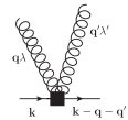
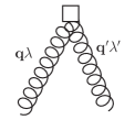
The second–order terms can be worked out in a similar way leading to the final form for their contribution to the electron–phonon interaction Hamiltonian:
(38)
In Eq. (38) we have introduced the functions and whose definition is quite similar to Eq. (36) and
Eq. (37)
(39)
(40)
with the reference nucleus–nucleus potential written in the
phonon modes basis by plugging Eq. (28) into Eq. (24).
The explicit expressions for and for are given in Appendix A, Eqs. (140) and (141).
Finally, the total Hamiltonian , up to second order in the nuclear displacements, can be written as
(41)
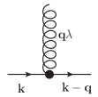
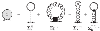
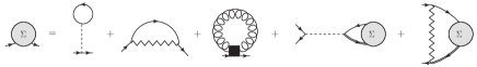
The diagrammatic transposition of the four electron–phonon interaction terms in Eq. (41) is given in Fig. (1). We see that we have two terms with
electronic legs ( and ). Those give direct contributions to the electronic propagator.
In addition, there are two purely nuclear contributions ( and ) that do not contribute directly to the electron propagator but
can be combined with the two electronic interactions and still contribute to the electronic self–energy, as it will be clear in the following.
Those are commonly neglected in textbook theories of the electron–phonon interaction.
But from Eq. (37) and Eq. (40) we see that there is no reason, a priori, to assume that both
and are zero.
The and interaction terms do not have electronic legs because they arise from the purely nuclear potential (). Nevertheless, at it is
evident from the above discussion, they can exchange momentum with the electronic subsytem. Energy, instead, is not exchanged as the nuclear potential is a static function. The momentum exchange
reflects the change in the nuclear–nuclear potential induced by a nuclear displacement. This term is neglected in the jellium model because, as it will be clear
in the following, the only allowed modes are acoustic excitations for which the zero frequency limit corresponds to the zero momentum limit. This contribution vanishes
as explained in Sec.V.1.1.
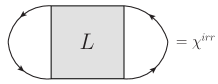
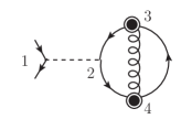
Figure 1:
Diagrammatic representations of the electron and phonon propagators (diagrams (a) and (b)) and of
the first (, diagram (c) and , diagram (d)) and second (, diagram (e) and , diagram (f)) order interaction terms in the Taylor expansion of
in powers of the nuclear displacements. All interaction terms are written in the basis of the phonon displacements.
More definitions can be found in the text.
Thus, any coherent and accurate framework that aims at providing a consistent way of introducing screening and correlation in the perturbative expansion of
Eq. (41) will also have to answer to the key question about the role played by the nucleus–nucleus interaction.
V The perturbative expansion
Now that the total Hamiltonian has been split in the bare Hamiltonian, Eq. (31), and in the interaction contributions,
, (Eq. (35)),
and (Eq. (38)), it is possible to perform a standard diagrammatic
analysis. In the following, we will work in the finite temperature regime where
the electronic Green’s function is defined Fetter and Walecka (1971) as
(42)
In Eq. (42) and is the temperature. represents the time ordering product,
the operator is written in the Heisenberg representation,
, with the chemical potential
and the total electronic number operator. We have introduced global variables to represent space and time components .
The average spanned by the trace operator runs over all possible interacting states weighted by the density operator .
By using Eq. (29), we can expand the Green’s function in the electronic basis defined by the reference Hamiltonian:
(43)
with
(44)
The electronic Green’s function can also be expressed in a matrix representation as
(45)
We will later use the same generic representation of Eqs. (43),(44) and (45) for the self–energy operator.
The non–interacting electronic Green’s function is diagonal in the band index and it reduces to a simple exponentialFetter and Walecka (1971)
(46)
with the Fermi-Dirac distribution function.
A similar expression holds for the non–interacting phonon propagator defined similarly to Eq. (42), with bosonic phonon operators replacing the
electronic ones :
(47)
with the Bose-Einstein distribution function.
Thanks to the standard many-body approach and perturbative expansion,
it is possible to rewrite in terms of and the electronic self–energy operator by means of
the Dyson equation Fetter and Walecka (1971)
(48)
where the matrix has been introduced following a definition similar to Eq. (45). Eq. (48) is written in
diagrammatic form in Fig.(2.a).
Note that in Eq. (48) the time variables and runs in the range .
In the following subsections we will write using approximations with an increasing level of correlation, self–consistency and screening in order to investigate the effect of the different electron-phonon interaction terms. The solution of the Dyson equation
corresponds to an infinite series in terms of the Green’s function and the self-energy.
Consistently with the harmonic approximation (the expansion with respect to the nuclear displacements is limited to the
second power in Eqs. (7) and (41)), we will work
up to second order with respect to , and only to first order in .
Higher orders of nuclear displacements
might appear as a consequence of self-consistency or screening (in the Dyson equation), but we will consider them to be negligible or to have no impact,
consistently with our choice of the harmonic approximation.
By contrast, for the electron-electron interaction, there will be no such approximation: higher-order powers of the electron-electron interaction will be significant.
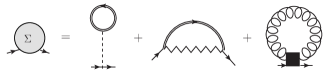
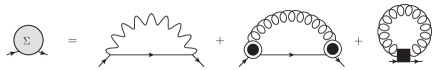
V.1 The Hartree, Debye–Waller and tad–poles self–energies
We analyze first the electronic self-energy that is obtained by considering only one interaction node attached to the electronic Green’s function, and select the lowest
non-vanishing diagrams. This self–energy can be obtained mathematically from the Feynmann diagrams in figure 2.b, following the diagrammatic rules of Ref. Fetter and Walecka, 1971, for example.
It is composed of four terms: the Hartree , Debye-Waller , nucleus-nucleus and electron-nucleus self-energy:
(49)
(50)
(51)
where .
The electron-phonon induced tad–pole contribution is
(52)
The other diagram (Fan diagram) appearing at second order in will be analyzed in the next subsection, Sec. V.2,
together with the Fock diagram from . They both have two interactions nodes attached to the electronic Green’s function.
The self-energy is the usual Hartree contribution which is a tad–pole diagram made of a Coulomb interaction that connects the incoming electronic propagator with another, closed,
electronic loop. Also the is a tad–pole diagram, but, in contrast to the Hartree term,
the interaction is not electronic but phonon mediated.
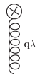
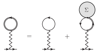
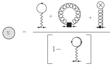
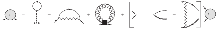
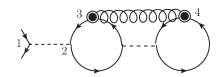
Figure 2:
Dyson equation written in terms of diagrams (frame (a)). In frame (b), instead,
the lowest-order electronic self–energy in the electron–electron and electron–phonon interaction is shown. We see the usual electronic Hartree contribution (first diagram) , the well-known
Debye–Waller term (second diagram) , and the electron–phonon induced tad–pole (fourth diagram) . In addition we see the
appearance of a new diagram due to the derivative of the nucleus–nucleus potential (third diagram), . This diagram plays a crucial role
in balancing the contribution from that, indeed, is not zero in general.
The nucleus-nucleus self-energy is a new term that has never been discussed before in the literature. It comes from the merging of a nucleus–nucleus and electron–nucleus interaction. It acquires an electronic character thanks to the contraction with the electronic propagator embodied in the electron–nucleus interaction ().
Finally is the well–known Debye–Waller (DW) self–energy. It represents the lowest (first) order electronic self–energy in the second–order derivative of the Hamiltonian.
The total self–energy is local in time and space and therefore the Dyson equation of Eq. (48) reduces to
(53)
with
(54)
The different contributions shown in Eq. (54) have the following properties:
(a)
All self–energy contributions are bare. No screening is present. This is not what should be applied for practical calculations because, as it will be clear
in the following, bare potentials lead also to unphysical properties.
Moreover from DFPT, we know that is screened.
In the original work of AHC this screening was introduced in a semi–empirical manner while in the more advanced
approach based on DFPTBaroni et al. (2001); Gonze (1995) the electron–nucleus interaction is screened in the self–consistent solution of the Kohn–Sham equation.
It is clear, however, that from a rigorous MB approach this screening is not present in the original Hamiltonian and must be build–up by the electronic correlations.
How does this screening emerge from a MB perspective?
(b)
The nucleus-nucleus self-energy is a new contribution that is not present in any treatment of the electron–phonon interaction where the nuclear density is approximated with an homogeneous charge density. In this work, the nuclear coordinates are instead coherently taken into account. This is an essential step to bridge the MBPT and DFT approaches.
(c)
In the standard approach to the electron–phonon interaction the electron-nucleus self-energy is commonly neglected. However the arguments that motivate this approximation Fetter and Walecka (1971) are based
on two specific approximations: (i) the nuclear interaction is dressed and (ii) there are only acoustic modes. In general, however, any system has both acoustic
and optical modes and the self–energy is not vanishing. What is its role and is it justified to neglect it?
In order to answer those questions we proceed with a detailed analysis of the two series of diagrams connected with the dressing of the tad–pole and of the Debye–Waller terms.
V.1.1 The electron–phonon induced tad–pole diagram and the nucleus–nucleus interaction contribution
The sum of the and is
(55)
This sum would be zero if the prefactor or if
the expression between brackets vanishes.
However the derivative of the bare ionic potential, when , diverges
like . Thus Eq.(55) is, actually, divergent.
In the Jellium model the
screening Fetter and Walecka (1971) of the electron–nucleus potential regularizes this divergence and
the dressed e–n interaction vanishes when . This is the standard motivation
used to neglect the contribution coming from the integral appering in the r.h.s of Eq.(55).
The term due to , instead, has been never considered before.
We focus our attention, instead, on the sum of the terms between brackets appearing in Eq. (55) for small but not vanishing values of . If we work it out we can rewrite it in a more clear way.
We notice that and, from Eq. (136) and Eq. (140), we have that
(56)
Before proceeding in the evaluation of Eq.(56) we notice that from the Dyson equation (Eq. (48)) it follows that
(57)
with the change in the Green’s function due to el–el correlation effects. Eq. (57) implies that
with the exact charge of the system with atoms frozen at the equilibrium positions.
Therefore, as in Eq. (56) , it follows that, within the harmonic approximation, we can safely assume
.
It follows than, that within the harmonic approximation,
the overlined quantity in Eq. (56) is minus the force acting on the nucleus located at
(58)
By using the Hellmann–Feynman theorem it follows that
(59)
with the exact electronic ground state of the total frozen Hamiltonian, .
Thus we can draw the following conclusion: if the self–energy is chosen in such a way that the nuclear positions and density correspond to the exact
electronic ground state
then it follows
(60)
This is true for the exact self–energy but it is not true for any approximation of the self–energy unless the Born-Oppenheimer energy of the
system is calculated accordingly by means of MBPT (for example by using the Luttinger–Ward expressions Fetter and Walecka (1971)).
The condition represented by Eq. (60) reveals the crucial role played by the nucleus–nucleus interaction. It is only thanks to the
coherent inclusion of electron-nucleus and nucleus-nucleus contributions that the theoretical framework can lead to the justification
of the AHC approach or to the textbooks results. A formal condition for the
tad–pole diagram to be zero can therefore be defined.
As an additional approximation we notice that one of the most widely approximation used in the litterature is to treat correlation effects non self–consistently. In pratice this means to use the
Dyson equation to renormalize the single particle energies but not the wave–functions. As a consequence, within this approximation, the charge density is assumed to be well described by the
one calculated within DFT. This approximation has an important and usefull consequence. Eq. (57) would impose to use as ionic positions ()
the ones calculated with a level of correlation coherent with the one introduced in . As this is a hardly (if not impossible) to
do in practice the use of the DFT charge allows to approximate both and in Eq. (58).
In this case are the DFT equilibrium atomic positions that are a simple by–product of any DFT calculation.
V.1.2 Self–consistent diagrams: dressing of the internal Green’s functions and of the bare interactions
Before starting the analysis of the diagrammatic structure of the self–energy we notice that at any order
of the diagrammatic expansion we can clearly distinguish between diagrams that dress the internal
electronic propagators and the interaction.
A clear definition of these two families of diagrams can be done
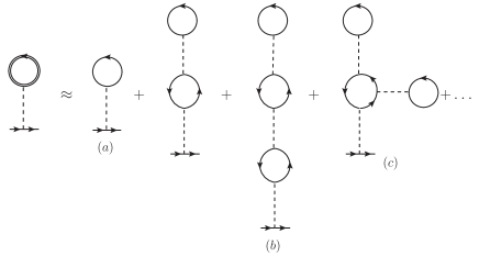
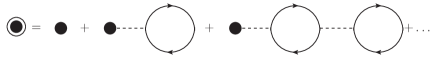
by using the simple Hartree approximation for the self–energy. Its diagrammatic expansion is shown in Fig.(3) and we notice that at third order, two different diagrams appear ( and ). In the case of diagram the interaction builds up a series of bubbles that describes electron–hole pair excitations. These bubbles, when summed to all orders,
reduce to the well–known Random Phase Approximation for the response function as it will be shown explicitly in Sec. (V.1.3).
The diagram , instead, represents a bare self–energy insertion in an internal Green’s function. Any other diagram where an internal propagator is dressed belongs to this family. The effect of these diagrams is to renormalize the single particle states. This can be easily visualized in the quasi–particle approximation where all internal propagator self–interaction contributions can be summed
in the definition of a new set of independent particle energies, .
In this work, we are interested in building up a scheme to concretely compare the Many–Body and DFT schemes as far as the e–n interaction is concerned. In order to greatly simplify the analysis, we will focus on the first series of diagrams disregarding all diagrams that correspond to a dressing of internal electronic propagators. In the self–consistent Hartree case this amounts to neglect
the diagram and, in practice, this means that the screening of the interaction is described by oscillations (described by bubble diagrams) of the bare charge. This approximation is commonly
used in the ai–MBPT scheme and can be written analytically as
(61)
When applied in the diagramatic context we will refer to Eq.(61) as the linearization procedure. The reason of the name will be clear in the next section.
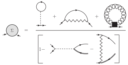
Figure 3: Diagrammatic expansion of the self–consistent Hartree self–energy. Diagram (a) is the non self–consistent contribution corresponding to the
bare electronic charge. Diagram (b) is composed of bare bubble diagrams. These diagrams belongs to the family of diagrams that dress the interaction. Diagram (c), instead, represents a dressing of the internal electronic propagator. All diagrams of this kind
can be, within the quasi–particle approximations, summed in a definition of a new independent particle Hamiltonian, as explained in the text.
V.1.3 Screening of the second–order electron-phonon interaction and of the Debye–Waller diagram
As mentioned earlier, one important aspect that must be included in the perturbative analysis in order to bridge it with
the DFPT formalism is the screening of the electron–phonon interaction terms.
How does screening build up ? This question could appear easy to answer as the series of diagrams that screen the lowest order () interaction is, indeed,
well known in the litterature. But, what about the second
order interaction, ?
In the original AHC work, the DW self–energy is written, from the beginning, in terms of a statically screened interaction.
However this screening cannot be introduced directly in the Hamiltonian. It must appear
as a result of the diagrammatic expansion.
In addition, from the discussion of the previous section, it follows that is not zero for any self–energy that does not
reproduce the exact reference density and the exact corresponding nuclear positions. As a matter of fact this is a condition hard to fulfill in any practical implementation as
it is computationally very difficult to find the nuclear positions corresponding to a specific level of approximation for .
Even if the condition given by Eq. (60) can be used as a simple approximation it is instructive, for the moment, to keep the two self–energies
in our derivation in order to see their effect on the definition of the screening.
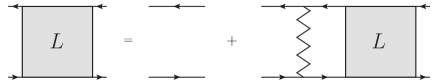
Figure 4:
The total bare interaction .
At the lowest order of the perturbative expansion the self–energy shown in Diagram 2.b can be explicitly written as
(62)
where we have introduced a total bare electron–electron interaction (see Fig. (4)) defined as
(63)
with the periodic –component of the Fourier transformation of the bare Coulomb interaction
(64)
with the integral restricted to the Brillouin Zone (BZ) only.
The total bare electron-electron interaction gets dressed (i.e. screened) by self-consistency when the Green’s function (Eq. (53)) is inserted into the self–energy (Eq. (62)). We can also sum over as the Hartree self–energy
is a local function and get
(65)
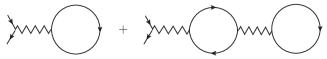
The term appearing in Eq.(62) is written in terms of Feynman diagrams in Fig.(5.a).
Now we group all operators to the left hand side of the equation.
We have that
(66)
and the corresponding diagrams are shown on Fig.(5.b).
Now, Eq. (66) is not linear in the sense that the right-hand side depends on the dressed because of the perturbative expansion of
the inverse of the square bracket quantity appearing in the left-hand side.
By using the discussion of Sec.V.1.2 we observe that all dressed
’s are internal Green’s functions. This can be deduced also by the expansion of the diagrammatic fraction appearing in Fig.(5.c). Then we can apply the linearization procedure, Eq.(61) to approximate with in the Eq.(66). This allows to define
the single–particle response function
(67)
Then, we define the dielectric matrix in the Time-Dependent Hartree approximation (see later) as
(68)
By using Eq. (66) into Eq. (67) the screening of the bare potential and
electron-phonon terms appears
so that
(69)
with , and the dressed counterparts of the bare , and functions
(70)
(71)
(72)
Eq. (69) and Eqs. (70), (71), (72) represent an important result of the present work. Indeed, they show that self–consistency screens
the interaction lines of all diagrams, including the Debye–Waller one. This result will be crucial in discussing how to include higher-order diagrams
avoiding double-counting problems.
Indeed, there are two well known ways of increasing the order of the perturbative expansion. One is to add skeleton diagrams and the other is to use
self–consistency. This second path is extremely important as it provides the way for a given self–energy to fulfill conserving conditionsStrinati (1988).
Skeleton (as well as reducible) diagrams are known to build–up the screening of the electron–electron and electron–nucleus interactions.
In this section we have shown that screening arises also from self–consistency.
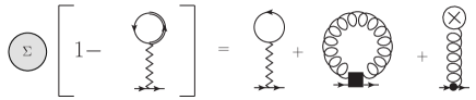
Figure 5:
Diagrammatic proof that self–consistency at the Hartree level is equivalent to screening, at the
time–dependent Hartree level. The proof is obtained by
using the Dyson equation inside the definition of the Hartree self–energy. This can be solved in terms of the self–energy
itself by a simple Fourier transformation because the Hartree self–energy is local in time. The mathematical transposition of
this proof is discussed in the text.
The first two diagrams resulting from the expansion of the diagrammatic fraction appearing in Fig. (5.c) are shown in Fig. 6.
The repeated closed loops represent the Time–Dependent Hartree (TDH) approximation for the response function. The corresponding screening of the interaction is known as
Random–Phase Approximation (RPA).
The RPA is the most elemental way to introduce screening in a system of correlated electrons.
Self–consistency dresses the electron-phonon interaction in the Hartree, in the tad–pole and in the DW diagrams. As it will be clear in the following,
the equation of motion for the corresponding screening function changes with the level of approximation used in the self–energy.
Moreover, when , the screening is due to the total time–dependent Hartree dielectric function that
includes the lattice polarization contribution. This follows from the definition of the zig–zag interaction, Fig. (4) and Eq. (63),
which induces (see Fig. (6), for example) scatterings processes where an electron–hole pair is annihilated and a phonon propagator is created.
Figure 6:
First two diagrams contributing to the screening of the Hartree (upper diagram) and DW (lower diagram) term. The screening can be written as the action of a
time–dependent Hartree screening function (see text). The dielectric function contains only the Hartree exchange diagrams as we considered only the Hartree term
in the electronic self–energy. However, it also includes phonon–mediated scatterings as a consequence of the fact that has been included in the diagrammatic expansion.
As it will be clear in the Sec. V.2, the addition of more diagrams to the electronic self–energy corresponds to modify the
equation of motion satisfied by the dielectric function.
Even today, most of the calculations at the level are performed by using the non self–consistent version.
However, this section shows that the DW diagram gets correctly screened only by solving the Dyson equation self–consistently.
V.2 The Fock and Fan self-energies
The analysis of the previous paragraph has been restricted at the Hartree level to keep the notation as simple as possible. In this section, we extend the derivation to the Fock approximation
by showing how the screening of the second–order electron-phonon interaction is modified by the inclusion of electronic exchange scatterings via the
Fock diagram. We will assume for simplicity that and show the changes that this approximation induces in the definition of the dielectric function.
The procedure to disentangle the self–consistency from the electron propagator appearing in the Fock operator can be done entirely using Feynman diagrams.
We start by using the Dyson equation to rewrite the dressed (thick line) electronic propagators in Fig. (7) in terms of the bare electronic propagators (thin line) and
of the self–energy. The resulting diagrammatic expression for is showed in Fig.(8.a).
Figure 7:
The Dyson equation at the Fock level in the electron–electron and electron–phonon interaction.
In addition to the Hartree and DW contributions we include the Fock diagram. Note that the zig–zag interaction lines
include the bare electron-phonon interaction defined in Fig.(4). Thus includes the DW and the Fan diagrams with bare and
un–dressed interactions.
We can then work out diagram (8.a) by isolating a non–local operator that is evidenced by the square brackets in the diagram (8.b).
The self–energy can be isolated to the left-hand side of the equation. Then, in the same spirit as for the
Hartree case, we can invert the equation. By following the same procedure used to go from diagram (5.b) to (5.c) we
introduce a diagrammatic fraction represented by the square bracket in the diagram (8.c). Formally speaking, this fraction must be
interpreted as follows. Let us consider the generic expression
, with and two generic diagrams with open interaction lines (in the present case
). Then we have that
(73)
where the sub–script means that, at each order, we consider the totally contracted products of and
in such a way that the resulting diagram has, again, open interaction lines.
We can illustrate this procedure by applying it to the DW term (last term in the numerator of diagram 8.c).
In this case, Eq. (73) applied to the square bracket produces an infinite series of diagrams that are closed in the upper part by a fermion
line contracted in the second–order bare interaction ().
The first three diagrams of this series are shown in Fig. (9.a).
The final result is
that, like in Sec.V.1.3, the Debye–Waller diagram is screened by a dielectric function. However, there are two important differences with respect to the Hartree case.
First of all, after linearization of the Green’s functions appearing in the right-hand side of the diagram (8.c) by using Eq. (61), we can define a different dielectric function than Eq. (68):
(74)
with the time–dependent Hartree–Fock irreducible response function. The equation that defines is represented in diagrammatic form in Fig. (9.b) and Fig. (9.c).
The corresponding definition of the screened second–order electron-phonon interaction is
Figure 8:
Diagrammatic proof of the equivalence between self–consistency and screening when a Fock and a Fan diagrams are present (second and third in
the r.h.s. of Fig.(7)). In the frame (b) a portion of the equation is isolated and enclosed in square brackets. By
defining formally the diagrammatic fraction (see text) the equation is inverted and the diagram in the square bracket goes
in the denonimator of frame (c). The perturbative expansion of this fraction leads to the screening of Hartree term and of
the second–order bare electron-phonon interaction . Some of the diagrams that follows from the expansion are shown
in Fig.(9).
The first two orders of are represented by the two bubbles
appearing in Fig.(9.a) while in Fig. (6) only the independent-particle bubbles appear (this is, indeed, the definition of the RPA).
In this case the Fock and Fan diagrams induce a first order bubble with the interaction connecting the two fermion propagators. This diagram represents the contribution of the electron–hole attraction and, when summed to all orders,
it can explain and predict the formation of excitonic statesOnida et al. (2002). Such bound electron–hole states are commonly observed in the absorption spectrum of several materials Onida et al. (2002).
In this case the electron–hole attraction is both electron and phonon mediated Marini (2008).
The second difference is the fact that in this derivation of the Hartree–Fock screening, we have assumed that the two tad-poles and cancel each other.
Formally speaking this cancellation is never exact. If the
contribution of these two terms is included then the dashed interaction in the denominator of the diagrammatic equation (8.c) would contain a electron-phonon contribution and
the whole definition of the screening function would be affected. This corresponds, for example, to the appearance of
exchange diagrams mediated by phonons.
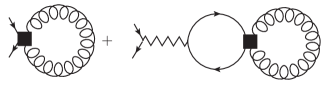
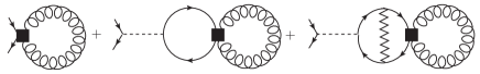
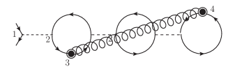
Figure 9:
The series corresponds to the first three diagrams contributing to the screening of the DW term. Similar series of diagrams contributing to the self–energy can be obtained by replacing the DW bare
self–energy with the Hartree and Fock self–energies. As we see besides the usual time–dependent Hartree contribution to the polarization
function (second diagram) there is a irreducible diagram where the electron and hole interact via the total screened interaction defined in
Eq. (63). The definition of the irreducible time–dependent Fock response function is given in the diagram in terms of the four point function . The final equation for
follows, then, from the corresponding equation of motion for (diagram ).
V.3 Skeleton diagrams, GW approximation and self–consistency issues
In Sec. V.1 and Sec. V.2 we have noticed that, even if we assume that tad–poles diagrams cancel each other, i.e. Eq. (60) is
satisfied, the screening of the first () and second ()
electron-phonon interaction potentials induced by self–consistency depends on the kind of approximation used for the electronic self–energy.
The situation for the other family of diagrams that must be considered at each order of the perturbative expansion is different. Indeed, if we consider
skeleton (bare) diagrams we have that the function is renormalized by the purely electronic dielectric function, as explained for example
in Ref. Mattuck, 1976 (via the diagrammatic method) and in Ref. van Leeuwen, 2004 (via the equation of motion approach):
(76)
In this case is the electronic dielectric function whose irreducible response function part follows directly by contracting the
vertex function associated with the self–energy. In the case of the well–known approximation, the dielectric function
is calculated within the RPA. The purely electronic expression can be obtained
from Eq. (68) when the phonon–mediated exchange
contribution is neglected and corresponds to approximate by .
Figure 10:
The Dyson equation at the GW level in the electron–electron and electron–phonon interaction. The electron–phonon diagram is known as Fan self–energy and its vertex (represented by the
circled dot) represents a dressed electron–phonon interaction (see Eq. (76)).
The wiggled line is a dressed electron–electron interaction (see Eq. (77)). The
most important aspect of this diagram is that, as long as only skeleton diagrams are included, the second–order electron-phonon interaction, and consequently the
DW diagram, is not screened.
The non self–consistent self–energy is showed in Fig. (10). The circled dot symbol () represents
the dressed interaction defined in Eq. (76) and, diagrammatically, in Fig. (11).
Similarly, the wiggled line is the screened electron–electron interaction
(77)
All the equations and definitions connected to the inclusion of skeleton diagrams are well–known in the literature. The original aspect outlined by the derivations presented in the previous sections is that, while
the first order electron-phonon interaction appearing in the Fan diagram is screened by skeleton diagrams, the second–order is screened by
self–consistency.
This deep difference in the procedure that defines the kind of screening of the electron-phonon interaction is reflected in the different equation that is satisfied by in, for example,
Eq. (77), Eq. (75) and Eq. (70). Depending on the choice of the self–energy, we have phonon mediated exchange and/or direct scatterings and electron–hole attraction diagrams.
We will see in the following that yet another family of dielectric functions is used within the DFPT approach. The
physical interpretation of these different definitions is discussed in Sec. VII.2.
Figure 11:
Diagramatic representation of the dressed electron–phonon vertex within the approximation for the self–energy. In this case the diagrams are bare (skeleton) and sum into an RPA dielectric screening
of the ionic potential. In this case, even in the case where the tad–pole diagrams are non zero, the dielectric screening is purely electronic. The standard additional approximation is to
consider a static screening.
VI The Density–Functional–Theory approach to the electron-phonon problem
In the previous section we have analyzed the kind of diagrams induced by the electron–electron interaction in the dressing of the
electron–nucleus interaction terms. We have disclosed the key role played by self–consistency and the different level of approximation that arises
from the perturbative expansion.
In order to link the DFPT and MBPT approaches we
start with a short review of the purely DFT–based approach to the electron–phonon coupling.
DFT is a self–consistent theory,
and DFPT is its extension to take into account, self–consistently, the effect of static perturbations (like nuclear displacements). In this
case, DPFT provides an exact description of phonons within the limits of a static and adiabatic approach. The phonon frequencies in DFPT are always real and no
phonon dissipation process is included.
If we introduce a total (electron–electron plus electron–nucleus) potential
(78)
where the functional dependence of the electronic density on the nuclear positions introduce a direct (via ) and
indirect (via ) dependence on in . In DFPT this complicated dependence links the calculation
of to the solution of a self–consistent set
of equations.
By applying the same procedure used to derive Eq. (7), a formal Taylor expansion of can be obtained.
However, if the dependence of the density on the nuclear positions is not taken into account,
all terms in the Taylor expansion are bare. In DFT (or DFPT), screening builds–up because of the
indirect dependence on . We introduce
(79)
and
(80)
The expression for can be written in terms
of by following the same procedure outlined in appendix A. The screening
of within a pure DFPT scheme follows from the fact that
(81)
In order to evaluate Eq. (81) and create a link with the MB approach, we notice that DFPT is based on the linear response
regime Baroni et al. (2001); Gonze (1995) where:
(82)
where the DFT polarizability is solution of the following Dyson equation
(83)
with the independent particle KS response function.
From the definition of the Hartree and xc potential it follows that
(84)
(85)
which, finally, yields the well-known expression for the derivative of the total DFT self–consistent potential
(86)
If we now introduce the DFT dielectric function
(87)
we have, finally, that
(88)
Similarly, the second–order derivative of can be introduced Gonze (1995); Baroni et al. (2001) as
(89)
Eqs. (88) and (89) must be compared with Eqs. (70), (71) and (72) in order to highlight the differences between the two formulations and potential similitudes.
Eq. (88) can be written in the basis of phonon displacements as
(90)
This last equation can directly be compared with Eq. (70) and the following observations can be made
(a)
In DFPT the function (and more generally the electron–phonon interaction) is statically screened and it does not include the contribution from the lattice polarization. In the MBPT, instead,
the electron-phonon interaction is dynamically screened (i.e. the dielectric functions defined in Eq. (68) and Eq. (74) are time dependent) and it includes
phonon mediated scatterings (see Eq. (70)).
The static screening of DFPT reflects the fact that there are no retardation effects in the theory. Those effects are peculiar of the MBPT and, in some cases, can
lead to important deviations from the static limit Cannuccia (2011); Cannuccia and Marini (2011b, 2012) when included in the self–energy.
(b)
The DFT dielectric function defined in Eq. (87) is a test–electron dielectric function whereas in the MBPT the dielectric function that screens the bare
electron-phonon interaction is a test–charge function. The difference between those two functions is well described in Ref. Hybertsen and Louie, 1987 and Ghosez et al., 1997. In the
test–charge case, the dielectric function represents a response to an external particle, while in the test–electron case, the charge is itself an electron. We will discuss in more detail this
difference from a physical perspective in Sec.VII.2.
(c)
A peculiar consequence of the DFPT approach is the appearance of non–rigid nuclei contributions to the second–order derivative of the electron–nucleus interaction potential,
. This contribution does not appear in the Many–Body derivation carried on in the previous sections.
Such non–rigid nuclei (recently called in the literature non–rigid ion contributionPoncé et al. (2014b)) can be studied by applying the derivative with respect to a nucleus displacement on the right-hand side of Eq. (89) and by distinguishing a rigid–nuclei (RN) and a non–rigid nuclei (NRN) terms
(91)
with
(92)
and
(93)
If we now rewrite both terms in the DFPT phonon basis and multiply by a pre factor we get
(94)
and
(95)
From the local dependence on of the it follows that, in the RN contribution, a appears. In the rigid–nuclei approximation
(also called the rigid-ion approximation) the is neglected.
The physical interpretation of the NRN contribution to the second–order derivative of the self–consistent potential is obscure in the DFPT derivation and
seems to be more a mathematical separation based on computational load of the calculations rather than a physically motivated choice (see Ref. Poncé et al., 2014b for a detailed explanation).
We will discuss this term from a Many–Body perspective in Sec. VII.3.
VII MBPT starting from Density–Functional and Density–Functional Perturbation Theory
The main difficulty in performing a diagrammatic expansion on top of DFT is that it is not possible to write the initial Hamiltonian in terms of
dressed interactions. This means that, even within DFT, the Taylor expansion of is still given by Eq. (32) with the only
difference that the electron–electron interaction is replaced by the mean–field xc–potential. At this point DFPT and MBPT follow two different routes in order to describe the dressing
of the interaction and the definition of the electronic self–energies.
To obtain the same screening as DFT+DFPT from a purely many–body point of view, we start by writing again the total Hamiltonian as a function of the KS one
(96)
We can determine the value of from Eqs. (17), (23) and (25)
(97)
with the equilibrium DFT density.
Now the full MBPT machinery described in the previous sections can be applied to Eq. (97), leading to the screening of the electron-phonon interactions. However, our aim is to create a link with
the DFPT definitions of Eq. (88) and (89). The main differences between the MBPT and DFPT approach
are listed in Table 1 and explained below.
Table 1: Schematic representation of the different treatment within MBPT and DFPT of the most important aspects of the electron–nucleus interaction.
Vanishing only when the atomic positions are evaluated consistently with the level of correlation included in the self–energy.
Vanishing.
Screening of the first order interaction, .
Time–dependent and described by a test–charge dielectric function consistent with the self–energy. Induced by skeleton diagrams.
Screened by the static test–electron DFT dielectric function. Introduced via self–consistency.
Screening of the second order interaction, .
Time–dependent and described by a test–charge dielectric function consistent with the self–energy. Induced by self–consistency diagrams.
Screened by the static test–electron DFT dielectric function. Introduced via self–consistency.
Non–rigid nuclei contribution to the second order interaction, .
Appears in the static limit from the diagrams that describe the dressing of the electronic density caused by the e–n interaction. It is, again, caused
by self–consistent diagrams.
Present and static. Induced by the implicit dependence of the screening on the atomic positions.
VII.1 Tad–Poles
By definition the DFT density is the exact one and it satisfies Eq. (58). Thus, bearing in mind the linearization procedure outlined at the end of Sec. V.1.1, we can affirm
that within DFPT, . As a consequence the dielectric function that screens the electron-phonon interaction does not include
phonon-mediated exchange scatterings.
VII.2 Screening of the second–order electron–nucleus interaction
In order to discuss how screening builds up, we start from the lowest order self–energy in the electron–phonon scattering (see Fig.(2.b)).
Again, we start from the bare Hamiltonian but this time we use the KS system as reference.
The Dyson equation that follows from
the Hamiltonian of Eq. (96) is
(98)
Moreover, since the Hartree part () also appears in , we have
(99)
In the case of a local self–energy, the difference of densities can be rewritten in terms of the self–energy by
using Eq. (53)
(100)
Following Eq. (68), we obtain within RPA and after linearization of the Green’s function () that
(101)
with
(102)
The final expression of the second–order electron-phonon interaction thus becomes
We notice that Eq. (104) defines a test–charge dielectric function while in DFPT, Eq. (87), a test–electron dielectric function appears.
This difference of definition is a straightforward consequence of the fact that the
definition of the dielectric function is linked to the distinction between the classical and the quantum parts of the induced potential.
The classical part satisfies a Poisson equation whose solution is the Hartree potential. The quantum part is treated in different ways in
MBPT and DFPT. In the MBPT, the quantum induced field is represented by the change of the
correlation self–energy due to a test charge. This is described by the vertex functionStrinati (1988) that can also be used to rewrite the exact self–energy in a closed form.
In DFT, instead, electronic correlations are included in a mean–field manner by means of the exchange–correlation potential. It follows that,
the variation of mimics the variation of the self–energy and, thus, represent the quantum part of the induced potential.
Therefore, the difference between a test–electron and a test–charge is that the test–electron includes the total variation of the total potential,
including . This contribution leads to the term appearing in the right-hand side of Eq. (87) and marks the difference between the
MBPT and DFPT screening.
As additional proof, we can notice that if the electronic self–energy is approximated with a DFT exchange–correlation potential, then
the many–body vertex turns the test–particle into a test–electron dielectric function that is
consistent with the DFPT definition. This means that is taking into account, in a mean–field manner, the effect of the MBPT vertex function.
At this point, we can conclude by observing that if local or semi–local approximations for are used, the difference between
a test–charge and a test–electron dielectric function can be safely neglected. Indeed any local or semi–local expression for
is regular in the short–distance limit whereas diverges. This means that, when , it follows that
.
More elaborate expressions for that also include proper short–distance spatial corrections exist.
In this case, a more accurate analysis of the effect of the Many–Body vertex function on the screening of the
electron-phonon interaction becomes essential to draw a conclusive parallel between MBPT and DFPT. However, this goes beyond the scope of the present work.
Therefore, as far as local or semi–local approximations for are used, we can approximate the DW screened interaction with the one evaluated at the DFPT level.
VII.3 The non–rigid nuclei contribution to the Debye–Waller self–energy from a diagrammatic perspective
One of the most undeniable difference between the DFT and MBPT scheme is the absence of a diagrammatic explanation for the non–rigid nuclei contribution (Eq. (95)) to the
second–order derivative of the nuclear potential. This terms has been shown to be quite important in low–dimensional systems Gonze et al. (2011) but, at first sight, it does not appear in
the many–body theory of the electron-phonon interaction. Indeed, in Eq. (71) and Eq. (75), the derivatives with respect to the atomic positions act only on the local bare ionic
potential.
In order to find a diagrammatic perspective of we follow again the path of performing a diagrammatic expansion
of the bare, un–dressed Hamiltonian and, at the end, draw links with DFT. In the present case we need to
to consider a new series of diagrams describing the change
of the electronic density induced by the electron–phonon interaction. Three examples of this series of diagrams are showed
in Fig. (12). We can see that those diagrams are of the same order of magnitude as the lowest
order self–energies and there is a priori no reason to neglect them.
Figure 12: First three diagrams that dress the Hartree self–energy due to the change of the electronic density induced by the
electron-phonon interaction. The sum of all diagrams of this kind (see Eq. (105) for a more formal definition) reduce, in the static and adiabatic limit, to the
NRN contribution to the Debye–Waller self–energy as discussed in the text.
The dressing of the Hartree self–energy can occur in two ways: the first is by dressing the internal electronic
propagators (an example is the Diagram (12.a)). The second way is to dress two tad–poles with phonon scatterings like in Diagrams (12.b)
and (12.c). All the diagrams of this kind can be written as
where is a first-order interaction that we assume to be screened by the very same skeleton diagrams that we
described in Sec.V.3.
In order to introduce a simple and clear interpretation of the contribution due to the diagrams, we take the static and adiabatic limit
of the atomic displacements. This approach will also simplify the connection with the corresponding quantity evaluated with the
DFPT scheme.
We start by taking the static limit of and of .
Moreover, in this limit, we can treat the
atomic displacements as classical and static variables in order to approximate
(109)
with the phonon displacements defined as
(110)
As we are interested in a specific series of diagrams, we can disregard higher-order corrections to .
The Eq. (109) allows to formally define
the derivative of the Green’s function, evaluated at the equilibrium nuclear positions. Indeed, from Eq. (109), it follows that
(111)
and
(112)
which, finally, using the identity
(113)
yields the desired definition
(114)
Eq. (114) is diagrammatically represented in Fig. (13). The derivative of the Green’s function splits the projector in two with the insertion
of a dressed electron-phonon first–order interaction ().
Figure 13: Diagrammatic transposition of the derivative of a Green’s function with respect to a specific displacement written in the phonon basis (see text, in particular Eq. (114)). The derivative
splits the Green’s function with the insertion of an electron-phonon first–order interaction.
By using Eq. (114) we notice that the first–order interactions appearing in the can be interpreted
as derivatives of the Green’s function.
By using Eq. (114) we can indeed rewrite the quantity in square brackets of Eq. (108) as
(115)
We take now the static limit of , which is consistent with the static and adiabatic approach taken in this section. In this way, we obtain the contribution of the first diagram (12.a) to
(116)
where the factor follows from the definition of (see Eq. (67)) that yields two equivalent contributions to .
If we now perform the same procedure to all bubble diagrams that contribute to time–dependent
Hartree reducible response function we get the diagram (12.b) and (12.c). The final expression for is
(117)
We have demonstrated that, in the static and adiabatic limit, the series of diagrams due to the dressing of the electronic density as a consequence of the
electron–nucleus interaction reduce to a new contribution to the series of second–order diagrams. However, the derivative with respect to the atomic displacements is acting on the dielectric function.
The Eq. (117) allows us to rewrite the DFPT NRN potential in a purely MBPT language.
A direct comparison between Eq. (117) and Eq. (95) reveals that the difference between the MBPT and the DFPT approaches lies in the dielectric function ( for the first and for the second).
VII.4 Screening of the first–order electron–nucleus interaction
If we now consider terms beyond the Hartree approximation, the definition of the dielectric function that screens the second–order interaction will change. This means that if we add to the
Hartree potential a Fock operator, a potential or a self–energy, the dielectric function will
solve a time–dependent Fock, DFT or GW equations.
We can anyway add new correlation terms to the self–energy by keeping frozen the self–consistency at the DFT level. This means that the dielectric function will approximatively
solve a DFT equation that, within the limits of the discussion of Sec. VII.2, will correspond to a simple RPA approximation written in the KS basis.
If we now include the Fan contribution to the total self–energy and
follow the same procedure already discussed for the skeleton diagrams (see Sec. V.3), we will obtain that the function is
renormalized by the standard skeleton polarization diagrams. These, again, will be summed in a RPA
dielectric function written in terms of KS bare Green’s functions.
VII.5 Self–consistency
As already mention earlier, the self–consistent diagrams play a crucial role in the definition of the second–order interaction.
The screening of the rigid–nuclei second–order interaction can be obtained with a simple self–consistent Hartree approximation (that is
already embodied in the DFT procedure). Instead, the non–rigid nuclei term requires to include, self–consistently, Fan diagrams and cannot be obtained with a simple
mean–field approximation.
This complicates the merging of MBPT and DFT as it is now clear that we can approximate the and
functions with the DFPT counterparts under the condition that the Dyson equation is not solved self–consistently. Any kind of
self–consistency would screen again the interaction leading to a severe over–screening.
The self–consistency must be taken from the solution of the KS equations and not re–introduced at the MB level. This, as explained above, will correspond to the inclusion of certain
class of diagrams, a practice that is well motivated within a many-body approach.
Finally, if the Dyson equation is not solved self–consistently, any additional electronic self–energy beyond the can be introduced as an additive potential (see Eq. (19)).
This means that it is safe to introduce non self–consistent quasi-particle corrections (electron and/or phonon mediated).
VII.6 Higher–order derivatives of the
The importance of creating a coherent merging of DFT and MBPT stems from the possibility of deriving an accurate and predictive approach to the electron-phonon interaction. There is however an entire family of physical problems induced by a strong electron–phonon interaction that requires to introduce higher-order self–energy diagrams.
A crucial difference with respect to the state–of–the–art models (like Fröhlich or Holstein Hamiltonians) is that the correct treatment of the
nuclear positions produce a new category of diagrams of generic order where the n–th order derivative of the
self–consistent potential appears
(118)
where the Debye–Waller diagram is the lowest order example.
Thanks to the simplicity of DFPT, it is possible to define an iterative expression for the matrix elements of
(119)
Such matrix can be rewritten in terms of and of the n–th derivative of the KS energy levels
(120)
with
(121)
and
(122)
where is a generic function of the atomic positions.
More information on Eq. (120) is provided in appendix B. Such procedure can be used to calculate numerically,
in an ab–initio manner, the high–order self–energies.
VIII Conclusions
In this work we have studied the electron–phonon problem by comparing
the standard Many–Body Perturbation Theory (MBPT) with Density Functional Theory (DFT) and Density Functional Perturbation Theory (DFPT).
By analyzing the different diagrams that contribute to the electronic self–energy we have achieved
several important goals.
(i) The well–known electron–phonon induced tad–pole diagram is not zero in general but can be cancelled by a nuclear–nuclear self–energy if
the equilibrium nuclear positions are coherent with the level of correlation introduced at the single–particle levels. In the case of
a non self–consistent calculation, the equilibrium positions evaluated with a DFT reference Hamiltonian removes the sum of the tad–pole diagrams.
(ii) Self–consistency diagrams dress the second–order interaction and the corresponding
Debye–Waller self–energy. This provides the many–body interpretation of the screened Debye–Waller self–energy already
known in the DFPT case.
(iii) We identify the specific series of diagrams that explain the non–rigid nuclei contribution to the Debye–Waller self–energy.
The existence of this term was known only in a purely DFPT (static and adiabatic) approach.
In the present work, we provide a clear
physical interpretation of this term by performing a static limit of the MBPT expression to
demonstrate that, indeed, it reduces to the well–known DFPT result.
(iv) We have drawn a final series of statements regarding the possibility
to perform many–body perturbation theory calculations on top of Density Functional and Density Functional Perturbation Theory avoiding
the double counting of diagrams.
This work represents a firm and formally accurate inspection of the two methods while describing the limitations of the static DFPT approach and providing
a practical way to go beyond by the merging with more advanced MBPT methods.
Acknowledgments
Financial support for AM was provided by the Futuro in Ricerca grant No. RBFR12SW0J of the
Italian Ministry of Education, University and Research.
SP and XG gratefully acknowledge support from FRS-FNRS through a FRIA grant (SP), and through the PDR Grant T.0238.13 - AIXPHO .
Appendix A The interaction Hamiltonians in the phonon displacements representation
We proceed here to discuss the details of the derivation and definition of the functions
(123)
(124)
(125)
(126)
where we purposely did not place a nucleus dependence on the left-hand side of those equations. We will indeed see that the dependence
is lifted by Eq. (131), as the derivatives have to be evaluated at .
Those functions enter in the different interaction terms of the electron-phonon interaction . We start by remembering that
(127)
and
(128)
It follows that
(129)
and
(130)
with and
. By using Eqs. (129) and (130) the
evaluation of the and is straightforward. It is enough to remember that
(131)
with a generic function. The resulting expression is therefore independent of .
The is then obtained by applying twice Eq. (131). We finally obtain that
(132)
The same machinery can be applied to obtaining:
(133)
Two important quantities follow from the integral of Eq. (132) and (133) when multiplied by two single–particle
wavefunction: and .
In order to evaluate those we have to consider, in the first-order derivative case, a term like
(134)
with the integral performed on the whole crystal. Now we observe that and depend on the atomic positions only via their argument.
If with the position of the atom inside the unit cell located at
we can change variable from to to center the sum in the unit cell corner. It follows that
Eq. (134) turns into
(135)
where is the periodic part of the wavefunction.
By using the fact that we finally obtain that
(136)
The same strategy can be used to define the matrix elements of :
(137)
The definition of is similar and follows directly from Eq. (126) and from the extension of Eqs. (129) and (130)
to the nucleus-nucleus potential:
(138)
and
(139)
This, leads to
(140)
and, finally, that
(141)
Appendix B An iterative expression for arbitrary n–th order derivatives of with respect to the nuclear displacements
One of the ingredients that are most difficult to calculate within an
ab–initio framework is the higher order derivatives of . While the first and second order are needed to calculate the lowest
order electron-phonon self–energies an extension of the theory to the regime of strong interaction requires the knowledge of an arbitrary order derivative
(142)
In order to derive a close expression for we use the following property of the nuclear momentum operator
(143)
This identity can be iterated to give:
(144)
More generally we have that
(145)
In order to evaluate the matrix elements we start by noticing that, within DFPT,
(146)
Now we define
(147)
and we plug into Eq. (145) a complete set of eigenstates obtaining
(148)
In order to rewrite in terms of we need to evaluate
In order to check the soundness of this approach we apply it to the first order case:
(151)
But it is easy to verify that
(152)
which implies that
(153)
Eq. (153),when used in Eq. (151), gives an identity
that confirms the correctness of the iterative equation, Eq. (150).
When Eq. (150) is applied to the second–order derivative it provides a well–known relation that connects the second to
the first derivative Poncé et al. (2014b); Gonze et al. (2011).
(154)
More in general Eq. (150) can efficiently rewrite the n–th order derivative in terms of the first order derivative and of the n–th order derivative of the
electronic energies,
.
But these derivatives can be efficiently calculated using DFPT or finite differences Poncé et al. (2014b); Antonius et al. (2014).
References
Ziman (1960)J. Ziman, Electrons and Phonons :
The Theory of Transport Phenomena in Solids (Oxford University Press, 1960).
Mitsuhashi et al. (2010)R. Mitsuhashi, Y. Suzuki,
Y. Yamanari, H. Mitamura, T. Kambe, N. Ikeda, H. Okamoto, A. Fujiwara, M. Yamaji, N. Kawasaki, Y. Maniwa, and Y. Kubozono, Nature 464, 76 (2010).
Allen and Cardona (1983)P. B. Allen and M. Cardona, Phys.
Rev. B 27, 4760
(1983).
Gosar and Choi (1966)P. Gosar and S.-i. Choi, Phys.
Rev. 150, 529 (1966).
Tamura et al. (2008)H. Tamura, J. Ramon,
E. Bittner, and I. Burghardt, Phys. Rev. Lett. 100, 107402 (2008).
Moser et al. (2013)S. Moser, L. Moreschini,
J. Jaćimović, O. S. Barisić, H. Berger, A. Magrez, Y. J. Chang, K. S. Kim, A. Bostwick,
E. Rotenberg, L. Forró, and M. Grioni, Phys. Rev. Lett. 110, 196403 (2013).
Cannuccia and Marini (2011a)E. Cannuccia and A. Marini, Phys.
Rev. Lett. 107, 255501
(2011a).
Cannuccia and Marini (2012)E. Cannuccia and A. Marini, The
European Physical Journal B 85, 1 (2012).
R.M.Dreizler and E.K.U.Gross (1990)R.M.Dreizler and E.K.U.Gross, Density Functional Theory (Springer-Verlag, 1990).
Onida et al. (2002)G. Onida, L. Reining, and A. Rubio, Rev. Mod. Phys. 74, 601 (2002).
Baroni et al. (1987)S. Baroni, P. Giannozzi, and A. Testa, Phys. Rev. Lett. 58, 1861 (1987).
Gonze (1997)X. Gonze, Phys.
Rev. B 55, 10337
(1997).
Baroni et al. (2001)S. Baroni, S. de Gironcoli, A. Dal
Corso, and P. Giannozzi, Rev. Mod. Phys. 73, 515
(2001).
van Schilfgaarde et al. (2006)M. van
Schilfgaarde, T. Kotani,
and S. Faleev, Phys. Rev. Lett. 96, 226402 (2006).
Gonze et al. (2011)X. Gonze, P. Boulanger, and M. Côté, Annalen der
Physik 523, 168
(2011).
Giustino et al. (2010)F. Giustino, S. G. Louie,
and M. L. Cohen, Phys. Rev. Lett. 105, 265501 (2010).
Poncé et al. (2014a)S. Poncé, G. Antonius,
P. Boulanger, E. Cannuccia, A. Marini, M. Côté, and X. Gonze, Computational Materials Science 83, 341 (2014a).
Antonius et al. (2014)G. Antonius, S. Poncé,
P. Boulanger, M. Côté, and X. Gonze, Phys. Rev. Lett. 112, 215501 (2014).
Keffer et al. (1968)C. Keffer, T. M. Hayes, and A. Bienenstock, Phys. Rev. Lett. 21, 1676 (1968).
Walter et al. (1970)J. P. Walter, R. R. L. Zucca, M. L. Cohen, and Y. R. Shen, Phys. Rev. Lett. 24, 102 (1970).
Kasowski (1973)R. V. Kasowski, Phys. Rev. B 8, 1378
(1973).
Allen and Heine (1976)P. B. Allen and V. Heine, Journal of Physics
C: Solid State Physics 9, 2305 (1976).
Allen and Cardona (1981)P. B. Allen and M. Cardona, Phys.
Rev. B 23, 1495
(1981).
Lautenschlager et al. (1985)P. Lautenschlager, P. B. Allen, and M. Cardona, Phys.
Rev. B 31, 2163
(1985).
Zollner et al. (1992)S. Zollner, M. Cardona, and S. Gopalan, Phys. Rev. B 45, 3376 (1992).
King-Smith et al. (1989)R. D. King-Smith, R. J. Needs, V. Heine, and M. J. Hodgson, EPL (Europhysics
Letters) 10, 569
(1989).
Franceschetti (2007)A. Franceschetti, Phys. Rev. B 76, 161301
(2007).
Kamisaka et al. (2008)H. Kamisaka, S. V. Kilina, K. Yamashita, and O. V. Prezhdo, The Journal of
Physical Chemistry C 112 (2008).
Ibrahim et al. (2008)Z. A. Ibrahim, A. I. Shkrebtii, M. J. G. Lee, K. Vynck, T. Teatro, W. Richter, T. Trepk, and T. Zettler, Phys. Rev. B 77, 125218 (2008).
Ramírez et al. (2006)R. Ramírez, C. P. Herrero, and E. R. Hernández, Phys. Rev. B 73, 245202
(2006).
Ramírez et al. (2008)R. Ramírez, C. P. Herrero, E. R. Hernández, and M. Cardona, Phys.
Rev. B 77, 045210
(2008).
Monserrat et al. (2013)B. Monserrat, N. D. Drummond, and R. J. Needs, Phys.
Rev. B 87, 144302
(2013).
Capaz et al. (2005)R. B. Capaz, C. D. Spataru,
P. Tangney, M. L. Cohen, and S. G. Louie, Phys. Rev. Lett. 94, 036801 (2005).
Patrick and Giustino (2013)C. E. Patrick and F. Giustino, Nature Communications 4 (2013).
Han and Bester (2013)P. Han and G. Bester, Phys. Rev. B 88, 165311 (2013).
Poncé et al. (2014b)S. Poncé, G. Antonius,
Y. Gillet, P. Boulanger, J. Laflamme Janssen, A. Marini, M. Côté, and X. Gonze, Phys. Rev. B 90, 214304 (2014b).
Kawai et al. (2014)H. Kawai, K. Yamashita,
E. Cannuccia, and A. Marini, Phys. Rev. B 89, 085202 (2014).
Marini (2008)A. Marini, Phys.
Rev. Lett. 101, 106405
(2008).
Mattuck (1976)R. Mattuck, A guide to Feynman
diagrams in the Many-Body problem (McGraw-Hill,
New York, 1976).
Fetter and Walecka (1971)A. L. Fetter and J. D. Walecka, Quantum theory of
many-particles systems (McGraw-Hill, 1971).