Improving the convergence properties of the moving-mesh code AREPO

Abstract

Accurate numerical solutions of the equations of hydrodynamics play an ever more important role in many fields of astrophysics. In this work, we reinvestigate the accuracy of the moving-mesh code Arepo and show how its convergence order can be improved for general problems. In particular, we clarify that for certain problems Arepo only reaches first-order convergence for its original formulation. This can be rectified by simple modifications we propose to the time integration scheme and the spatial gradient estimates of the code, both improving the accuracy of the code. We demonstrate that the new implementation is indeed second-order accurate under the $L^{1}$ norm, and in particular substantially improves conservation of angular momentum. Interestingly, whereas these improvements can significantly change the results of smooth test problems, we also find that cosmological simulations of galaxy formation are unaffected, demonstrating that the numerical errors eliminated by the new formulation do not impact these simulations. In contrast, simulations of binary stars followed over a large number of orbital times are strongly affected, as here it is particularly crucial to avoid a long-term build up of errors in angular momentum conservation.

1 Introduction

Gravity and hydrodynamics provide the foundations for describing almost all phenomena in astrophysics. Often, the dynamics and geometry are sufficiently complicated that analytic solutions, especially for hydrodynamics, cannot be obtained. These limitations can be overcome by numerical approaches, which have developed over the recent decades into powerful tools for studying complex hydrodynamical flow problems. It is however an ongoing and persistent challenge to derive ever better discretization schemes that reduce numerical discretization errors to a minimum, while at the same time offering high adaptivity to different time- and length-scales and a high degree of parallel scalability. Astrophysical code development is therefore best viewed as an iterative effort which never is fully complete and finished. Rather, new generations of numerical ‘instruments’ (i.e. codes) should ideally improve their accuracy and speed, somewhat similar in spirit to the advances regularly realized in observational instrumentation.

Traditionally, stationary mesh codes with or without adaptive mesh refinement (e.g. Fryxell et al., 2000; Teyssier, 2002; Almgren et al., 2010; Stone et al., 2008; Bryan et al., 2014) and smoothed particle hydrodynamics (SPH) codes (e.g. Wadsley et al., 2004; Springel, 2005) have dominated astrophysical fluid dynamics. Moving meshes and hybrid techniques combining Eulerian and Lagrangian meshes have been applied only rarely in astrophysics and related fields (e.g. Hirt et al., 1974; Gnedin, 1995; Pen, 1998). However, in particular in astrophysics they have not seen widespread use so far.

Recently, moving-mesh techniques based on a Voronoi mesh have been proposed (Springel, 2010; Duffell & MacFadyen, 2011), which offer a quasi-Lagrangian description that inherits some of the advantages of SPH while retaining the accuracy of a Eulerian mesh-based description. These new methods have matured into interesting alternative codes that have already been widely applied in cosmological simulations of structure formation (e.g. Vogelsberger et al., 2012; Sijacki et al., 2012; Marinacci et al., 2013; Vogelsberger et al., 2014; Genel et al., 2014), as well as in first star formation (e.g. Greif et al., 2011, 2012; Smith et al., 2014), and to a smaller extent in stellar astrophysics (Pakmor et al., 2013) and in problems related to planet formation (Duffell & MacFadyen, 2012; Muñoz et al., 2014, 2015). It has become clear that it can be very worthwhile to accept the technical complications introduced by a dynamic and unstructured mesh given the benefits realized by combining most of the advantages of fixed mesh codes (e.g. better convergence for smooth flows, good shock capturing) and SPH techniques (e.g. intrinsic adaptivity, lack of advection errors, small numerical diffusion).

A well-defined and rapid convergence rate is a particularly important feature of mesh codes, which are usually constructed to be at least second-order accurate for smooth flows, i.e. in the absence of shocks or other discontinuities. For SPH codes, in contrast, it is very hard to demonstrate proper convergence in the first place (Zhu et al., 2015). In practice, the convergence rate dictates how rapidly a numerical solution improves as more computational effort is invested, an aspect that is arguably even more important than the absolute size of the error itself. For example, while SPH often obtains a qualitatively correct result with acceptable error at low resolution, its poor convergence rate does not allow it to reach comparable accuracy to mesh codes at comparable numerical cost once the resolution is high. In contrast state of the art mesh-based codes are expected to show at least second order convergence.

Moving-meshes in general have been studied extensively (see, e.g. Thomas & Lombard, 1979; Guillard & Farhat, 2000). In this paper, we reexamine the accuracy and convergence rate of the Arepo code (Springel, 2010), which is at present the most widely employed implementation of the moving-mesh technique in astrophysics. We address weaknesses in the original version of this code and show how they can be overcome to improve the overall accuracy of the scheme. This directly affects the range of applicability of the code and is hence important for further maturing the moving-mesh approach in general.

The paper is structured as follows. In Section 2, we concisely review the essential parts of the implementation of moving-mesh hydrodynamics in Arepo and analyse its convergence. In Sections 3 and 4, we describe improvements to the time integration scheme and the gradient estimate, respectively. We apply the new implementation to test problems in Section 5, show results for realistic applications in Section 6, and discuss the implications of our work in Section 7.

2 Moving-mesh hydrodynamics in Arepo

The moving-mesh code Arepo solves the Euler equations using the finite-volume approach on an unstructured Voronoi mesh that is generated from a set of points (Springel, 2010). At any given time during the simulation, the mesh can be uniquely constructed given only the positions of the mesh-generating points. Since the mesh-generating points move, the geometry of the mesh and its connectivity change over time.

The Euler equations can be written as a system of hyperbolic conservation laws for conserved quantities U and a flux function $\textbf{F}(\textbf{U})$,

$$\frac{\partial\textbf{U}}{\partial t}+\nabla\cdot\textbf{F}=0.$$ (1)

For the standard Euler equations the conserved quantities are mass, momentum and energy. They define a vector of conserved quantities and an associated flux function as

$$\textbf{U}=\left(\begin{array}[]{c}\rho\\ \rho\textbf{v}\\ \rho e\end{array}\right),\ \ \ \ \ \ \ \textbf{F}(\textbf{U})=\left(\begin{array}[]{c}\rho\textbf{v}\\ \rho\textbf{v}\textbf{v}^{T}+P\\ \rho e\textbf{v}+P\textbf{v}\end{array}\right),$$ (2)

where $\rho$, v, $P$, and $e$ are density, velocity, pressure, and total specific energy of the fluid, respectively. The latter is defined as the sum of the specific internal energy $u$ and the specific kinetic energy $\frac{1}{2}\textbf{v}^{2}$, thus $e=u+\frac{1}{2}\textbf{v}^{2}$. The system of equation is closed by an equation of state $P=\rho(\gamma-1)e$ with the adiabatic index $\gamma$.

To solve the Euler equations, the state of the fluid is discretised using the cells of the Voronoi mesh. To this end, averages of the conserved quantities U of the fluid are computed for each cell through integration over the finite volume of a cell $i$,

$$\textbf{Q}_{i}=\int_{V_{i}}\textbf{U}\,\mathrm{d}V.$$ (3)

yielding a census of the conserved physical quantities in the cell. This state is then evolved in time by

$$\textbf{Q}_{i}^{n+1}=\textbf{Q}_{i}^{n}-\Delta t\sum_{j}A_{ij}\mathbf{\hat{F}}_{ij}^{n+1/2},$$ (4)

where $A_{ij}$ is the oriented area of the face between cells $i$ and $j$ and $\mathbf{\hat{F}}$ is a time-averaged approximation of the true flux $\textbf{F}_{ij}$ across the interface between cells $i$ and $j$.

The calculation of the fluxes $\mathbf{\hat{F}}$ is done in the original version of Arepo using a MUSCL-Hancock scheme (van Leer, 1984; Toro, 1999), which has been shown to provide second-order accuracy in time and space for all kinds of stationary meshes (see, e.g. Fryxell et al., 2000). This method uses a slope-limited piece-wise linear spatial reconstruction step in each cell and a first order time extrapolation of the fluid states by half a timestep to obtain the states on both sides of all interfaces. Finally, a Riemann solver uses the states on both sides of an interface to compute the flux that is exchanged during the timestep.

The extrapolation is carried out in primitive variables

$$\textbf{W}=\left(\begin{array}[]{c}\rho\\ \textbf{v}\\ P\end{array}\right),$$ (5)

which are straightforwardly calculated from the conserved quantities and the geometry of a cell with the equation of state, combined with estimates for their local spatial gradients. By construction, they represent the values at the center of mass of a cell. Then, the left and right states of an interface are computed by a linear spatial extrapolation from the center of mass $\mathbf{s}$ of a cell to the center $\mathbf{f}$ of a cell face, and by a half-step prediction forward in time (where $\Delta t$ is the full timestep) as

$$\textbf{W}^{\prime}_{\mathrm{L,R}}=\textbf{W}_{\mathrm{L,R}}+\left.\frac{\partial\textbf{W}}{\partial\textbf{r}}\right|_{\mathrm{L,R}}\left(\mathbf{f}-\mathbf{s}_{\mathrm{L,R}}\right)+\left.\frac{\partial\textbf{W}}{\partial\textbf{t}}\right|_{\mathrm{L,R}}\frac{\Delta t}{2}.$$ (6)

The time derivatives of the primitive variables in Eqn. (6) are not calculated directly. Instead, the Euler equations are used to express them in terms of the primitive variables and their spatial derivatives only:

$$\frac{\partial\rho}{\partial t} = -\textbf{v}\nabla\rho-\rho\nabla\textbf{v},$$ (7)

$$\frac{\partial\textbf{v}}{\partial t} = -\frac{\nabla P}{\rho}-\textbf{v}\nabla\textbf{v}^{T},$$ (8)

$$\frac{\partial P}{\partial t} = -\gamma P\nabla\textbf{v}-\textbf{v}\nabla P.$$ (9)

The extrapolation and computation of the fluxes over an interface are all done in the rest frame of the (moving) interface, i.e. the interface velocity is subtracted from the equations above. This allows solutions that are manifestly Galilean-invariant, an important conceptual advantage over traditional Eulerian methods where the numerical truncation error grows with the fluid velocity.

In the original implementation of Arepo, the spatial gradients are calculated using an improved Green-Gauss estimator that makes use of certain mathematical properties of the Voronoi mesh. Specifically, the gradient estimate for a primitive variable $\phi$ in cell $i$ is given by

$$\left<\nabla\phi\right>_{i}=\frac{1}{V_{i}}\sum_{j}A_{ij}\left(\left[\phi_{j}-\phi_{i}\right]\frac{\textbf{c}_{ij}}{r_{ij}}-\frac{\phi_{i}+\phi_{j}}{2}\frac{\textbf{r}_{ij}}{r_{ij}}\right),$$ (10)

where

$$\textbf{c}_{ij}=\frac{1}{A_{ij}}\int_{A_{ij}}\left(\textbf{r}-\frac{\textbf{r}_{i}+\textbf{r}_{j}}{2}\right)\mathrm{d}A$$ (11)

is the center of mass of the face between $i$ and $j$, and $\textbf{r}_{ij}=\textbf{r}_{i}-\textbf{r}_{j}$ is the difference between the positions of the mesh-generation points of cells $i$ and $j$, and $r_{ij}=\left|\textbf{r}_{ij}\right|$ is its length. The sum runs over all cells that share an interface with cell $i$. Note that this estimate of the spatial gradient of a primitive variable depends only on the values of the primitive variable in the cell itself and its direct neighbours, and on the local geometry of the cell. If the values of the primitive variables sample an underlying smooth field at the positions of the mesh-generating points, then the gradient estimate is second-order accurate for an arbitrary mesh geometry, i.e. it reproduces a constant gradient in the field to machine precision. However, the primitive variables Q used to compute the gradient estimates represent volume averaged quantities rather than the value of the fluid at the mesh generating point of a cell.

Figure 1: $L^{1}$ norm of the density field as a function of the number of resolution elements per dimension at $t=10$ for the isentropic Yee vortex, simulated with the standard Arepo implementation using MUSCL-Hancock time integration and the improved Green-Gauss gradient estimates.

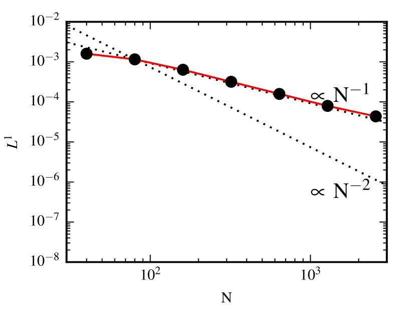
In the original AREPO implementation of Springel (2010), all computations that require geometrical quantities, e.g. volumes, areas, or positions of face centroids, use the geometry of the mesh at the beginning of the timestep. Nevertheless, it has been argued that the scheme is second-order accurate, based on simple sound-wave tests (Springel, 2010) using the $L^{1}$ norm, and based on the much more-demanding stationary isentropic vortex flow (Yee et al., 2000), where the error decreases quadratically with increasing spatial resolution (Springel, 2011).

In this paper, we define the $L^{p}$ norm of a continuous field as

$$L^{p}=\left(\frac{1}{V}\int_{V}\left|f\left(\textbf{r}\right)\right|^{p}\mathrm{d}V\right)^{1/p},$$ (12)

where $f\left(\textbf{r}\right)$ is, for example, the deviation of the density field from its analytical value at a position r. For our finite volume discretisation this becomes

$$L^{p}=\left(\frac{1}{V}\sum_{i=1}^{N_{\mathrm{cells}}}\left|f_{i}\right|^{p}V_{i}\right)^{1/p}.$$ (13)

The $L^{1}$ norm of the density field for the Yee vortex (for the detailed setup, see Appendix A) evolved until $t=10$ with the original AREPO code is shown in Figure 1. In contrast to previous claims, the error only decreases linearly with resolution, i.e. AREPO shows first order convergence only. The difference to previous results (in particular Springel, 2011) arises from an inappropriate definition of the $L^{2}$-norm employed there.

On static Cartesian meshes, we find that Arepo is fully second order convergent for smooth problems. On moving meshes, however, an inaccuracy is introduced since the time integration only uses the geometry of the mesh at the beginning of the timestep, ignoring changes of the mesh geometry during a timestep. One possibility to account for these changes in the time integration is to do an additional mesh construction at the middle of the timestep and use the geometrical properties at $t=t_{0}+\Delta t/2$ to calculate the fluxes. However, this requires at least one further (expensive) mesh construction per timestep, nearly doubling the computational cost. Such an approach combined with a Runge-Kutta time integration scheme is followed in Tess (Duffell & MacFadyen, 2011).

3 Runge-Kutta time integration

Alternatively, one can abandon the MUSCL-Hancock scheme and try to use a different Runge-Kutta time integration scheme that avoids a mid-step mesh construction. Of particular interest for us is Heun’s method, which is a second-order Runge-Kutta variant that calculates the flux as an average of the fluxes at the beginning and the end of the timestep. Applying Heun’s method to our moving mesh leads to the following update equations of the conservative variables for a cell $i$

$$\textbf{Q}^{\prime}_{i} = \textbf{Q}^{n}_{i}-\Delta t\sum_{j}A^{n}_{ij}\mathbf{\hat{F}}_{ij}^{n}\left(\textbf{U}^{n}\right),$$ (14)

$$\textbf{r}^{\prime} = \textbf{r}^{n}+\Delta t\,\textbf{w}^{n},$$ (15)

$$\textbf{Q}^{n+1}_{i} = \textbf{Q}^{n}_{i}-$$ (16)

$$\frac{\Delta t}{2}\,\left(\sum_{j}A^{n}_{ij}\mathbf{\hat{F}}_{ij}^{n}\left(\textbf{U}^{n}\right)+\sum_{j}A^{\prime}_{ij}\mathbf{\hat{F}}_{ij}^{\prime}\left(\textbf{U}^{\prime}\right)\right),$$

$$\textbf{r}^{n+1} = \textbf{r}^{n}+\frac{\Delta t}{2}\,\left(\textbf{w}^{n}+\textbf{w}^{\prime}\right).$$ (17)

Here, the vectors r denote again the coordinates of the mesh-generating points, w their velocities, and $\mathbf{\hat{F}}_{ij}$ is an approximation for the fluxes of the conserved variables over the interface between cells $i$ and $j$. In principle it is possible to allow the velocities of the mesh-generating points to change during a timestep (Duffell & MacFadyen, 2011), but we choose to always keep them constant over the course of a full timestep.

Note that this update rule also requires the geometry of two different meshes ($\textbf{r}^{n}$ and $\textbf{r}^{\prime}$), and the fluxes have to be computed twice for every timestep. However, since for Heun’s scheme and a constant velocity $\textbf{w}^{\prime}=\textbf{w}^{n}$ of the mesh-generating points over the whole timestep we can show that

$$\textbf{r}^{n+1}=\textbf{r}^{n}+\frac{\Delta t}{2}\,\left(\textbf{w}^{n}+\textbf{w}^{\prime}\right)=\textbf{r}^{n}+\Delta t\,\textbf{w}^{n}=\textbf{r}^{\prime},$$ (18)

we can reuse the mesh we constructed for the second half of the current timestep for the first half of the next timestep. Thus, we only need to construct the mesh effectively once per timestep, which keeps the mesh construction effort equal to Arepo’s original implementation. The fluxes need to be calculated twice as often, but the computational cost required for this is a relatively small effort compared to the 3D mesh construction needed in a moving-mesh code, and therefore does not increase the overall computational cost significantly.

In practice, computing the intermediate state $\textbf{Q}^{\prime}$ through Eqn. (14) is inconvenient for several reasons. In particular, it significantly complicates the internal bookkeeping of the conserved variables since we need to know $\textbf{Q}^{n}_{i}$ and $\textbf{Q}^{\prime}_{i}$ at the same time in Eqn. (16). While this can be resolved in principle, further complications arise when one tries to consistently implement this update scheme for individual time steps that vary locally.

These problems can be circumvented in a simple way by extrapolating to the intermediate step using spatial derivatives, like in the previous MUSCL-Hancock scheme. This leads to an update of the conservative variables through

$$\textbf{W}^{\prime}_{i} = \textbf{W}^{n}_{i}+\Delta t\,\frac{\partial\textbf{W}}{\partial\textbf{t}},$$ (19)

$$\textbf{r}^{\prime} = \textbf{r}^{n}+\Delta t\,\textbf{w}^{n},$$ (20)

$$\textbf{Q}^{n+1}_{i} = \textbf{Q}^{n}_{i}-$$

$$\frac{\Delta t}{2}\,\left(\sum_{j}A^{n}_{ij}\mathbf{\hat{F}}_{ij}^{n}\left(\textbf{W}^{n}\right)+\sum_{j}A^{\prime}_{ij}\mathbf{\hat{F}}_{ij}^{\prime}\left(\textbf{W}^{\prime}\right)\right),$$

$$\textbf{r}^{n+1} = \textbf{r}^{\prime}.$$ (22)

Here, we only need to do the time extrapolation for the primitive variables, and we again use the Euler equations to replace time derivatives with spatial derivatives. Note that this update scheme can be easily generalized to local individual time steps. For the calculation of the fluxes between two cells on different time steps, the time extrapolation (Eqn. 19) is in this case done for each cell always from the last time the cell was active. At this time the estimates for its primitive variables and gradients were obtained. Similarly, the linear spatial extrapolation to the current center of the interface is always done from the center of mass for which primitive variables and their gradients have been calculated. Note, that with the time-extrapolation to the intermediate step our scheme is not a Runge-Kutta scheme anymore, but becomes a hybrid between Runge-Kutta and MUSCL-Hancock schemes.

4 Least square gradient estimates

Another source of accuracy degradation in the original Arepo implementation lies in the quality of the gradient estimates, which can suffer in general problems. The issue appears when a cell is distorted and its mesh-generating point deviates significantly from the position of the center of mass of the cell. In this case, the Voronoi-optimized Green-Gauss estimate of Eqn. (10) introduces a systematic error, because it assumes that the primitive variables are known at the mesh-generating points, whereas, by construction, the primitive variables represent volume-averaged quantities that represent the value of the underlying field at the cell’s center-of-mass. Although the small steering motions added by Arepo to the velocities of the mesh generating points usually manage to keep the mesh nicely regular with only a small offset between the mesh-generating point and the center-of-mass of a cell, the typical distance between these two points can amount to a few percent of the radius of the cell, enough to significantly degrade the accuracy of the gradient estimate in some situations.

Figure 2: $L^{1}$ error norm of the Voronoi-optimized Green-Gauss gradient estimate of the density field for different types of meshes for the initial state of the Yee vortex at $t=0$.

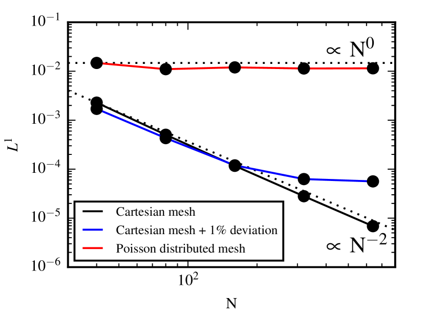
We investigate this in Fig. 2 explicitly, where we show that such a small deviation already compromises the accuracy of the gradient estimate, spoiling its convergence rate for higher resolutions. In fact, a one percent deviation of the mesh-generating points from the centers of mass in an almost Cartesian mesh already stops the improvement of the gradient estimate with resolution for resolutions better than $320^{2}$ cells. Even worse, for a completely random mesh in which the mesh-generating points are a Poisson sample of the simulation domain the gradient estimate does not improve with resolution at all. Note, however, that the hydro scheme still converges with first order, even though the error in the gradient estimate is constant.

To more robustly reach second-order convergence of the hydrodynamical scheme, we therefore need better gradient estimates that are correct to at least first order for severely distorted meshes where center-of-mass values are known, equivalent to requiring that linear gradients are still reproduced exactly in this case.

Figure 3: $L^{1}$ norm of the least-square-fit gradient estimate of the density field for different types of meshes for the initial state of the Yee vortex at $t=0$.

Assuming that we know the local geometry of the mesh and the values of a quantity $\phi$ at the centroids of the cells, we can obtain such a gradient estimate through a local least squares fit. We note that polynomial least squares reconstructions are well known for unstructured meshes, and form a standard technique in particular for high-order ENO and WENO schemes (e.g. Ollivier-Gooch, 1997). Also, such methods are well known for the estimation of gradients (e.g. Maron & Howes, 2003). They have also been recently used for SPH and in new variants of mesh-less methods (Hopkins, 2014) and to compute the cell-centered magnetic fields in constrained transport schemes for unstructured meshes (Mocz et al., 2014). The method assumes that the quantity $\phi$ can be approximated everywhere within cell $i$ as

$$\phi\left(\textbf{r}\right)=\phi\left(\textbf{s}_{i}\right)+\left<\nabla\phi\right>_{i}\left(\textbf{r}-\textbf{s}_{i}\right).$$ (23)

The value of $\phi$ at the center of mass of the cell $\phi\left(\textbf{s}_{i}\right)\equiv\phi_{i}$ is known as a prerequisite, and we are now looking for an estimate of the gradient $\left<\nabla\phi\right>_{i}$. We also know $\phi$ at the centres of mass of all neighbouring cells $j$, so we can require that our gradient estimate reproduces those $\phi_{j}$ as well as possible. Thus, for every neighbouring cell, we would like to have

$$\phi_{j}=\phi_{i}+\left<\nabla\phi\right>_{i}\left(\textbf{s}_{j}-\textbf{s}_{i}\right).$$ (24)

For $N$ neighbouring cells this is an overdetermined set of $N$ equations with only up to three free variables (or two in 2D). We select the best linear approximation for $\left<\nabla\phi\right>_{i}$ by requiring that it minimises the sum of the deviations for all neighbours,

$$S_{\mathrm{{tot}}}=\sum_{j}g_{j}\left(\phi_{j}-\phi_{i}-\left<\nabla\phi\right>_{i}\left(\textbf{s}_{j}-\textbf{s}_{i}\right)\right)^{2}.$$ (25)

Here, $g_{j}$ is the relative weight for neighbor $j$. Different choices for these weights are possible, but according to our experiments the results are not very sensitive to the particular choice made. We follow de Vasconcellos & da Silva (2014) and set it to $g_{j}=A_{ij}/\left|\textbf{s}_{j}-\textbf{s}_{i}\right|^{2}$.

To minimise $S_{\mathrm{{tot}}}$, we use the normal equations which yield

$$\hskip 28.45274pt\sum_{j}g_{j}\textbf{n}_{ji}\otimes\textbf{n}_{ji}\left<\nabla\phi\right>_{i}\left|\textbf{s}_{j}-\textbf{s}_{i}\right|^{2}=$$

$$\;\;\;\sum_{j}g_{j}\left(\phi_{j}-\phi_{i}\right)\textbf{n}_{ji}\left|\textbf{s}_{j}-\textbf{s}_{i}\right|,$$ (26)

where $\textbf{n}_{ji}=\left(\textbf{s}_{j}-\textbf{s}_{i}\right)/\left|\textbf{s}_{j}-\textbf{s}_{i}\right|$. This corresponds to a $2\times 2$ or $3\times 3$ matrix inversion problem in two- or three-dimensional problems, respectively, which can be solved by an appropriate solver to obtain $\left<\nabla\phi\right>_{i}$.

Figure 4: $L^{1}$ norm of the density field for the evolved Yee vortex at $t=10$ when different schemes for the hydrodynamics are employed. For the detailed setup of the Yee vortex problem see Appendix A.

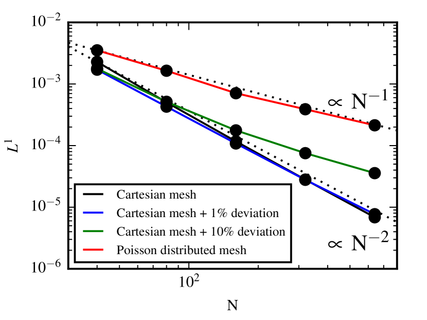
The accuracy of the new least squares fit gradient estimate is shown in Fig. 3. On the nearly Cartesian mesh examined earlier, the gradient estimate is as accurate as the Voronoi-optimized Green-Gauss estimate. For increasing deviations from the Cartesian mesh, the accuracy of the least squares gradient estimate slowly deteriorates, but importantly, it never becomes worse than first order. In particular, even for the random mesh it still accurately recovers the linear gradient, unlike the Voronoi-optimized Green-Gauss estimate.

5 Test problems

To examine the difference between the original Arepo implementation that employs a MUSCL-Hancock time integration scheme (MH) and the Voronoi-adjusted Green-Gauss gradient estimate (GG) versus the Runge-Kutta time integrator (RK) combined with the least squares gradient estimator (LSF), we compare these schemes for several representative test problems. In obtaining the results for the different implementations, we always use identical code configurations, parameters, and initial conditions, and only vary the time integration method and/or gradient estimate.

All test problems in this paper are run using a Courant factor of $0.3$ to determine the timestep and employ the same strategy and parameters to evolve the mesh while keeping it regular. To regularise the mesh, the mesh-generating points are moved towards the center of mass of their cell. Their total velocity is calculated as

$$\textbf{v}_{\mathrm{vertex}}=\textbf{v}-\frac{1}{2}\Delta t\frac{\nabla P}{\rho}+\textbf{v}_{\mathrm{reg}}$$ (27)

where v, $P$, $\rho$, $\Delta t$, and $\textbf{v}_{\mathrm{reg}}$ are the fluid velocity, pressure, and density, timestep of the cell, and a regularisation component that is added purely to improve the mesh. It is given by

$$\textbf{v}_{\mathrm{reg}}=\epsilon\max\left(c,r\,\left|\nabla\times\textbf{v}\right|\right)\frac{\textbf{d}}{\left|\textbf{d}\right|}.$$ (28)

Here, $c$ is the sound speed in the cell, $r$ the approximate extent of the cell calculated from its area (volume) in 2D (3D) assuming the cell is a circle (sphere), and $\textbf{d}=\textbf{r}-\textbf{s}$ is the separation between mesh-generating point and center of mass of the cell. Note that this separation is interesting in its own right, as it can be used to quantify the regularity of the mesh. Moreover, $\epsilon$ is defined as

$$\epsilon=\max\left(0,\min\left(0.5,0.5\,\frac{\alpha-0.75\beta}{0.25\beta}\right)\right)$$ (29)

and $\alpha$ is given by

$$\alpha=\max_{i}\left(\frac{1}{N_{\mathrm{dim}}}\frac{2A_{i}}{\left|\textbf{r}-\textbf{r}_{i}\right|}\right),$$ (30)

where the maximum runs over all neighbours of a cell and their interfaces connecting a cell to them. We choose the parameter $\beta$ to be 2.25 in all simulations in this paper.

Figure 5: Conservation of total angular momentum for the Yee vortex at $t=10$ when different hydrodynamical schemes are used.

Figure 6: Density error compared to the analytical solution (top panel) and relative separation between mesh-generating point and center of mass (bottom panel) at $t=100$ for the RKLSF Yee vortex.

5.1 Yee vortex

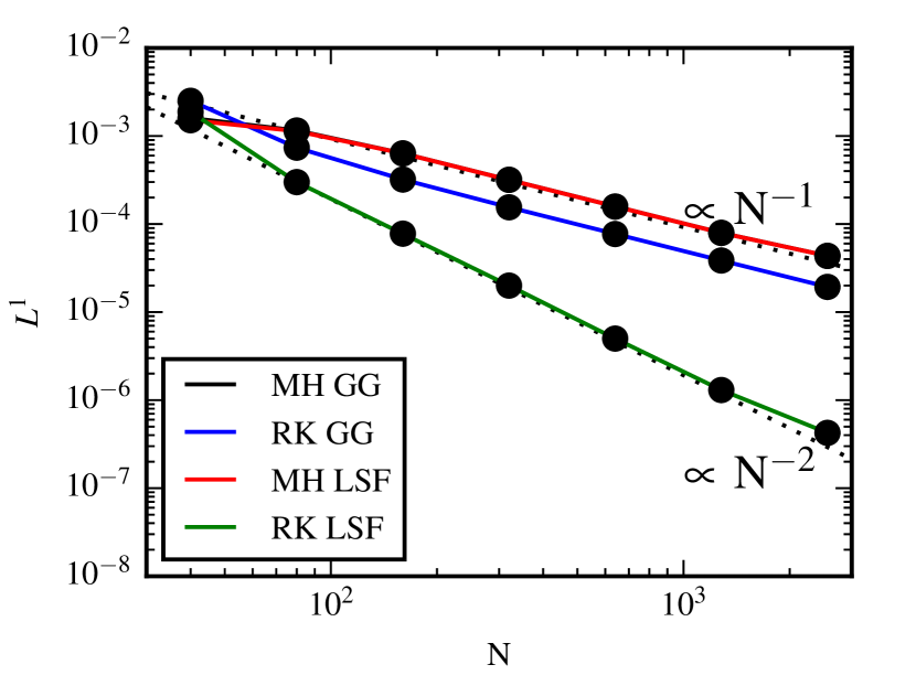
We first reevaluate the convergence rate for the isentropic Yee vortex. Since this vortex flow is completely smooth, we in principle expect to see second-order convergence in the strong $L^{1}$ norm if the implementation is correct. As shown in Fig. 4, we indeed obtain second-order convergence up to very high resolution for Arepo in the moving-mesh case if we use both the least squares gradient estimate and the Runge-Kutta time integration scheme. Using only one of the two improvements while keeping the MUSCL-Hancock integration scheme or the improved Green-Gauss gradient estimate, respectively, does not change the convergence rate at all and makes the implementation drop back to first-order convergence in the $L^{1}$ norm. The detailed setup including the initial mesh can be found in Appendix A.

Figure 7: Evolution of the surface density of a two-dimensional cold Keplerian disc. The top panels show the initial conditions and the evolved state at $t=100$ obtained with the original Arepo implementation based on the improved Green-Gauss gradient estimate and the MUSCL-Hancock time integration. The bottom panels show the new implementation with least squares gradient estimate and Runge-Kutta time integration at $t=100$ and $t=600$, respectively. At the latter time, the inner disc has finished more than $250$ orbits. The detailed setup can be found in Appendix B.

It is interesting to note that the Tess code has been shown to be second-order accurate for an isentropic sound wave with a Runge-Kutta time integration scheme (Duffell & MacFadyen, 2011), while the same Voronoi-optimized Green-Gauss gradient estimate as implemented originally in Arepo has been used. With this gradient estimate, the convergence order is however expected to break down for meshes in which the mesh-generating points are not close to the centers of mass of their cells. The difference here is most likely that the one-dimensional propagation of the wave in this particular problem only stretches the mesh, without displacing the mesh-generating points from the centres of mass of their cells. As discussed before, in this special case the Voronoi-optimized gradient estimate is sufficient and does not negatively impact the convergence properties. For the more demanding Yee vortex this is not the case, however, and the convergence is expected to break down in Tess just as in the original Arepo code.

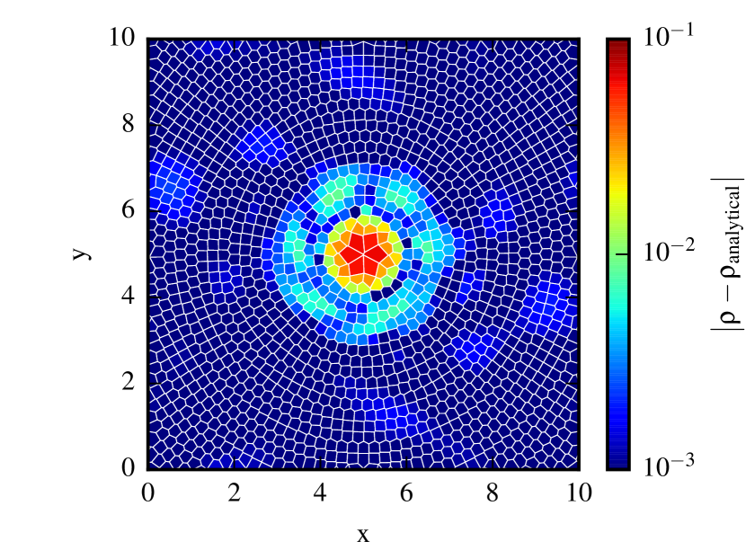
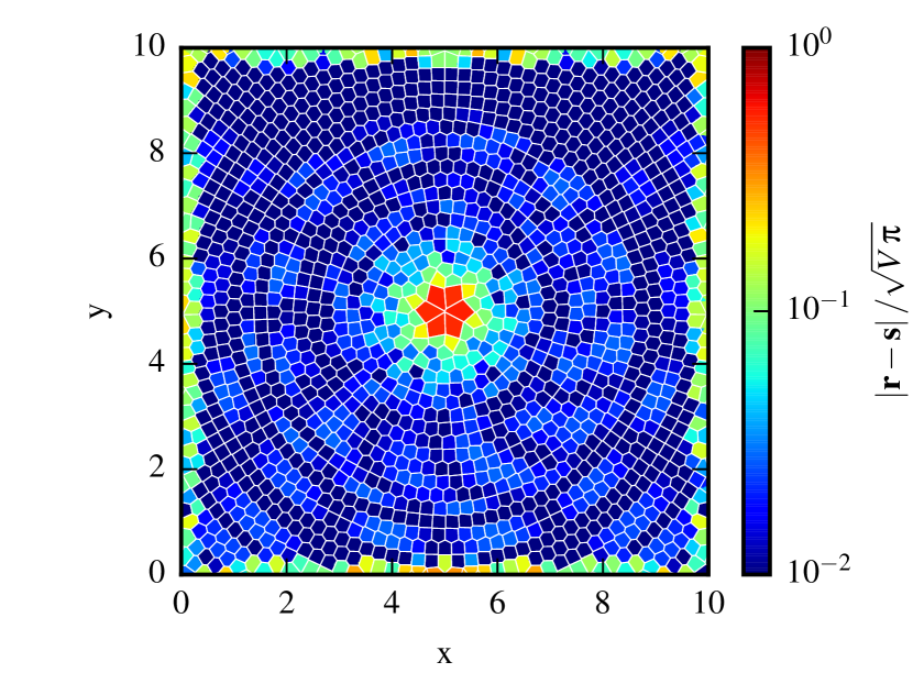
Another interesting observation to make is that second-order convergence in Arepo for the new implementation as measured by computing the $L^{1}$ norm between the current density field and the analytical solution is only reached at very high resolution when the initial mesh-generating points are set up in rings around the center of the vortex. If an initially Cartesian mesh is adopted instead, the convergence degrades to first order at sufficiently high resolution. As shown in Fig. 6 there is only a weak correlation between the density error in a cell and its distortion, as both are largest close to the center of the vortex.

This is fundamentally caused by the discretization of the analytical problem onto our mesh. There are two discretizations involved, a first discreziation on the initial mesh to generate the discretized initial conditions and a second discretization on the current mesh when we measure the $L^{1}$ norm. If the structure of the mesh changes systematically between the initial and the current mesh, there is also a systematic difference in the two discretizations, which turns out to lead to a first order error that dominates the total error at sufficiently high resolution. Because an initially Cartesian mesh will eventually be transformed to a spherical mesh by the mesh regularization, the measured $L^{1}$ norm after the mesh changed will not be better than first order at high resolution. To overcome this problem, we arrange the mesh-generating points in the initial mesh already on circles around the center of the vortex. This mesh configuration is stable for the problem, thus there is no systematic change in the discretisation over time.

Another approach is to look at error measures intrinsic to the discrete problem that do not require a second discretisation of the analytical problem. Analysing the conservation of total angular momentum (which also may be viewed as a norm) instead of the $L^{1}$ norm of the total density field is therefore considerably simpler and also more robust. In particular, here the measured convergence rate is independent of the initial mesh, and the rearrangement from an initially Cartesian to a circular mesh does not give rise to additional errors. As shown in Fig. 5, the angular momentum conservation is again only improved if both, a better time integration method and a more accurate gradient estimate, are used. Interestingly, the angular momentum even shows third order convergence in the new implementation, although this may be the result of the special spherical symmetry of the vortex flow and may be lost for more general problems.

5.2 Keplerian disc

Evolving a cold Keplerian disc for many orbits is a common problem in astrophysics, with applications from planetary to galactic discs. Using such a set-up in the limit of a pressure-less gas disc is a demanding test problem (Cullen & Dehnen, 2010; Hopkins, 2014). In fact, as highlighted by Hopkins (2014), many state-of-the-art static mesh or SPH codes have severe problems in coping accurately with this situation. Instead, the disc is typically destroyed during the first $10$ orbits by these methods.

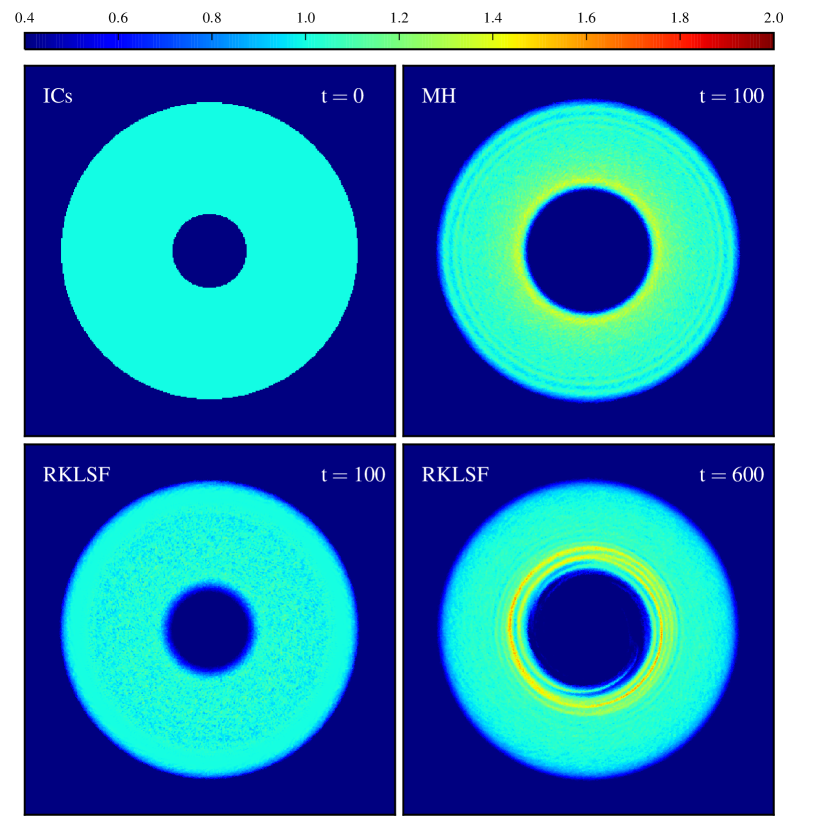
The original AREPO code with the MUSCL-Hancock time integration and improved Green-Gauss gradients already does quite well on this problem, as shown in Fig. 7 where we display the disc after roughly $15$ inner orbits with a resolution of 320x320 cells. However, whereas the outer parts of the disc are very stable, the inner boundary of the disc moves outwards with time owing to systematic errors in angular momentum conservation. Our new implementation with Runge-Kutta time integration and least squares gradients works significantly better, keeping the disc essentially perfectly stable until $t=100$, and showing similar errors only much later, at times $t\simeq 600$ or later. These residual errors can now be much more efficiently improved to essentially arbitrary precision by an increase of the spatial resolution, thanks to the improved convergence order. This is in line with previous results on conservation of angular momentum in AREPO for more realistic problems (Muñoz et al., 2015).

These results compare very favourably not only to stationary Eulerian grid codes on Cartesian meshes, but also to the new mesh-free hydrodynamical method proposed by Hopkins (2014). Note, however, that the optimal mesh configuration for this specific problem is most likely a polar grid.

6 Testing on realistic applications

6.1 Evolution of a stellar binary

In light of our previous results, it is interesting to investigate whether the improvements in the Arepo code proposed here affect the results of real world scientific applications of the code. Compared to the Yee vortex and the Keplerian disc, which are smooth hydrodynamics-only problems, or hydrodynamical problems with a constant external gravitational field, one example of a more complex problem including discontinuities, shocks, and self-gravity is the inspiral and merger of a close binary system of two white dwarfs.

Such simulations are essential to understanding the complex evolution of the merger process and to determining the fate of the binary system (see, e.g. Zhu et al., 2013; Pakmor et al., 2013; Dan et al., 2014). The initial mesh for the white dwarfs is constructed from shells that are tesselated using the HEALPIX algorithm to obtain regular cells with roughly the same mass (Pakmor et al., 2012). The simulation box is then filled by a low resolution Cartesian background grid. Figure 8 shows the total angular momentum for the merger of two white dwarfs with masses of $0.65\mathrm{M_{\odot}}$ and $0.625\mathrm{M_{\odot}}$, an initial orbital period of $44$ s, identical to the setup of the same system in Zhu et al. (2013). We employ a mass resolution of $10^{-6}\mathrm{M_{\odot}}$ (high resolution) and $5\,10^{-6}\mathrm{M_{\odot}}$ (low resolution), respectively.

Figure 8: Conservation of total angular momentum for the merger of two white dwarfs with an initial orbital period of $44$s for the MUSCL-Hancock time integration and improved Green-Gauss gradient estimate and the Runge-Kutta time integration combined with the least squares gradient estimate.

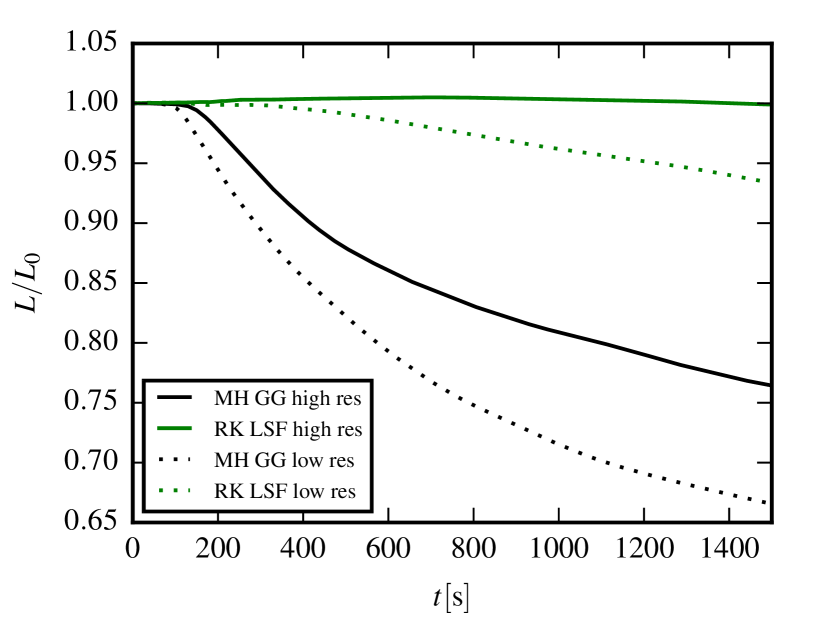
The binary merges at around $t=200\,{\rm s}$, after initial mass transfer reduced the separation and lead to runaway mass transfer. It then forms a differentially rotating merger remnant. The differential rotation in the merger remnant is crucial for its further evolution. As shown in Figure 8, conservation of angular momentum during the further evolution of the merger remnant is significantly violated for the implementation with MUSCL-Hancock time integration and improved Green-Gauss gradient estimates. The system loses a significant fraction of the total angular momentum present in the simulation. In contrast, the new implementation with Runge-Kutta time integration and least squares gradient estimates conserves the total angular momentum in the simulation to a relative error of about one percent even after many orbits for the high resolution simulation and still loses less than $10\%$ of the total angular momentum in the low resolution simulation.

Figure 9: Comparison of two cosmological zoom runs of a galaxy similar to the Milky-Way (as in Marinacci et al., 2013) using either the combination of MUSCL-Hancock time integration and improved Green-Gauss gradient estimate, or the combination of Runge-Kutta time integration and least squares gradient estimate, respectively. Initial conditions, code configuration and parameters including all sub-grid physics are identical for both runs and chosen in line with Marinacci et al. (2013) and Pakmor et al. (2014). The top row shows, from left to right, stellar projections of the two runs at $z=0$ and the evolution of the star formation rate in the disc of the main galaxy. The bottom row shows circularities of stars in the disc, evolution of the total mass of the halo compared to its stellar mass, and the average root mean square magnetic field strength in the disc for the two runs.

6.2 Cosmological zoom simulation of galaxy formation

An even more complex problem are simulations of galaxy formation and evolution. They not only involve self-gravity, but also feature high Mach numbers and turbulent flows, as well as a large number of additional source terms to model effects like radiative cooling of gas or the energy injection of evolving stars. In addition, sometimes explicit sub-grid models for unresolved physics are used that are introduced as a modified equation of state or pressure floors and the like.

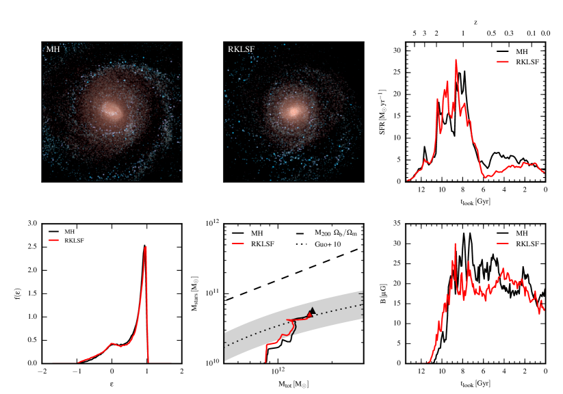
To compare the performance of our new code with the original Arepo version in this regime we have repeated one of the recent Milky Way galaxy formation simulations of Marinacci et al. (2013) and Pakmor et al. (2014). These are advanced calculations that can serve as an example for current state of the art simulations of cosmic structure formation (see, e.g. Agertz et al., 2011; Scannapieco et al., 2012; Stinson et al., 2013; Hopkins et al., 2014; Vogelsberger et al., 2014; Schaye et al., 2015; Khandai et al., 2015). As shown in the results overview of Fig. 9, there is no significant difference between the results obtained for both implementations.

A possible interpretation of the lack of differences for the cosmological runs is that the properties of galaxies and their dynamics are already captured sufficiently accurately by the standard Arepo implementation. The accuracy improvements brought about by the new formulation proposed here are either irrelevant for this problem, or are completely dominated by first order errors introduced by the sub-grid models for radiative cooling, star formation, and feedback. The latter is particularly likely as it is now well understood that the outcome of galaxy formation simulations depends very sensitively on the treatment of highly non-linear feedback processes. Thus, in regions of the simulation that are crucially shaped by feedback we do not expect our improvements to the code to lead to significant changes of the results. Changing this to improve the solution requires implementing and coupling the source terms such that the combined system is second order accurate. This may be different in regions where hydrodynamics and gravity are the only relevant phenomena. For example, conceivably some differences may be found in the approximately hydrostatic atmosphere of rich galaxy clusters, where our new formulation may result in a marginally better representation of turbulence.

7 Conclusions

In this paper, we have discussed in detail two simple modifications of the cosmological moving-mesh code Arepo, which are nevertheless quite important to recover full second-order convergence in the $L^{1}$ norm for general smooth problems with non-trivial mesh motions. One of these changes concerns the time integration, where a Runge-Kutta time integration scheme is adopted instead of the MUSCL-Hancock approach in order to account for changes of the mesh geometry during a timestep at second order. This does not increase the number of mesh-constructions needed, but does double the number of required flux computations. The other change is the adoption of a more general (and slightly more expensive) gradient estimate that retains the necessary accuracy even for large offsets between the mesh-generating points and the centers of masses of cells.

These improvements are most relevant for smooth, pure hydrodynamics problems where the influence of self-gravity and of complicated source terms is limited. Among the astrophysical problems that fall into this regime and that have already been tackled with the original version of Arepo are proto-planetary discs (Muñoz et al., 2014), cold gas in galactic discs (Smith et al., 2014), and dynamical stellar mergers (Pakmor et al., 2013). Such simulations and similar problems will benefit in the future from the added accuracy facilitated by the improvements proposed here. It is also prudent to carry out additional tests to see whether previous simulations were sometimes degradated in a noticeable way by an accuracy loss of the code, for example by an unnecessarily large error in the conservation of angular momentum. We expect such noticeable errors only for problems that evolve a system for many dynamical timescales.

Cosmological simulations of galaxy formation seem to be unaffected by the improvements of the hydrodynamical moving-mesh scheme proposed here. This is of course reassuring as it means that previous results from galaxy formation studies carried out with Arepo, both with zoom-in techniques (Marinacci et al., 2013; Pakmor et al., 2014) and in large cosmological boxes (Vogelsberger et al., 2014; Genel et al., 2014), have not suffered from the convergence rate issues discussed above. Nevertheless, it is clearly desirable to use the improved scheme in the future in this regime as well, especially since it offers higher accuracy at an insignificant increase of the computational cost.

Appendix A Yee Vortex

For the setup of the Yee vortex we follow Yee et al. (2000). The mesh is defined on the domain $\left[-5,5\right]\times\left[-5,5\right]$. In the initial conditions, we set density $\rho$, velocity v, and specific internal energy $u$ of the cells to the value of the continuous fields at the centres of mass of the cells. The continuous fields at position $\textbf{r}=\left(x,y\right)$ are given by

$$T\left(\textbf{r}\right) = T_{\inf}-\frac{\left(\gamma-1\right)\beta^{2}}{8\gamma\pi^{2}}e^{1-r^{2}},$$

$$\rho\left(\textbf{r}\right) = T^{\frac{1}{1-\gamma}},$$

$$v_{x}\left(\textbf{r}\right) = -y\frac{\beta}{2\pi}e^{\frac{1-r^{2}}{2}},$$

$$v_{y}\left(\textbf{r}\right) = x\frac{\beta}{2\pi}e^{\frac{1-r^{2}}{2}},$$

$$u\left(\textbf{r}\right) = \frac{T}{\gamma-1}.$$

We choose the parameters as $T_{\inf}=1$, $\gamma=1.4$, and $\beta=5$.

The setup of a Cartesian mesh is trivial. To organise the mesh-generating points on rings around the center of the vortex in a regular way, we first compute the width of a ring as $d_{\mathrm{ring}}=10/N$, where $10$ is the size of our domain in one dimension and $N$ the linear resolution. We then add mesh-generating points on circles with radii that are multiples of the width of a ring, $r_{\mathrm{ring}}=i\times d_{\mathrm{ring}}$. On every circle we equidistantly add $2\pi\,r_{\mathrm{ring}}/d_{\mathrm{ring}}$ points. We only add points that lie in the computational domain and repeat this until none of the points of a new ring are in the domain anymore.

Appendix B Keplerian Disc

The setup for the Keplerian disc is similar to the one used in Hopkins (2014). We use a computational domain of $\left[-2.5,2.5\right]\times\left[-2.5,2.5\right]$. The disc is cold, i.e. the pressure support is negligible compared to gravitational force and orbital velocity. The initial mesh is again organised on rings around the center of the disk. We set the initial surface density $\rho$, velocity v, and specific internal energy $u$ of the cells to the values of the continuous fields at the centres of mass of the cells. The continuous fields at position $\textbf{r}=\left(x,y\right)$ and $r\equiv\left|r\right|$ are given as follows. For $r<0.5$ and $r>2$ we set

$$\rho = 10^{-5},$$

v $$= 0,$$

$$u = \frac{5\gamma}{2\rho}\times 10^{-5}.$$

And for $0.5\leq r\leq 2$ we adopt

$$\rho = 1.0,$$

$$v_{x} = -\frac{y}{r}\sqrt{\frac{1}{r}},$$

$$v_{y} = \frac{x}{r}\sqrt{\frac{1}{r}},$$

$$u = \frac{5\gamma}{2\rho}\times 10^{-5}.$$

We choose an adiabatic index of $\gamma=5/3$. The constant external gravitational acceleration is given by

$$\textbf{g}=-\frac{\textbf{r}}{r\left(r^{2}+\epsilon^{2}\right)},$$ (31)

where $\epsilon=0.25$ for $r<0.25$ and $\epsilon=0$ everywhere else.

References

- Agertz et al. (2011) Agertz O., Teyssier R., Moore B., 2011, MNRAS, 410, 1391
- Almgren et al. (2010) Almgren A. S., et al., 2010, ApJ, 715, 1221
- Bryan et al. (2014) Bryan G. L., et al., 2014, ApJS, 211, 19
- Cullen & Dehnen (2010) Cullen L., Dehnen W., 2010, MNRAS, 408, 669
- Dan et al. (2014) Dan M., Rosswog S., Brüggen M., Podsiadlowski P., 2014, MNRAS, 438, 14
- Duffell & MacFadyen (2011) Duffell P. C., MacFadyen A. I., 2011, ApJS, 197, 15
- Duffell & MacFadyen (2012) Duffell P. C., MacFadyen A. I., 2012, ApJ, 755, 7
- Fryxell et al. (2000) Fryxell B., et al., 2000, ApJS, 131, 273
- Genel et al. (2014) Genel S., et al., 2014, MNRAS, 445, 175
- Gnedin (1995) Gnedin N. Y., 1995, ApJS, 97, 231
- Greif et al. (2011) Greif T. H., Springel V., White S. D. M., Glover S. C. O., Clark P. C., Smith R. J., Klessen R. S., Bromm V., 2011, ApJ, 737, 75
- Greif et al. (2012) Greif T. H., Bromm V., Clark P. C., Glover S. C. O., Smith R. J., Klessen R. S., Yoshida N., Springel V., 2012, MNRAS, 424, 399
- Guillard & Farhat (2000) Guillard H., Farhat C., 2000, Computer Methods in Applied Mechanics and Engineering, 190, 1467
- Hirt et al. (1974) Hirt C. W., Amsden A. A., Cook J. L., 1974, JCP, 14, 227
- Hopkins (2014) Hopkins P. F., 2014, preprint, (arXiv:1409.7395)
- Hopkins et al. (2014) Hopkins P. F., Kereš D., Oñorbe J., Faucher-Giguère C.-A., Quataert E., Murray N., Bullock J. S., 2014, MNRAS, 445, 581
- Khandai et al. (2015) Khandai N., Di Matteo T., Croft R., Wilkins S., Feng Y., Tucker E., DeGraf C., Liu M.-S., 2015, MNRAS, 450, 1349
- Marinacci et al. (2013) Marinacci F., Pakmor R., Springel V., 2013, MNRAS,
- Maron & Howes (2003) Maron J. L., Howes G. G., 2003, ApJ, 595, 564
- Mocz et al. (2014) Mocz P., Vogelsberger M., Hernquist L., 2014, MNRAS, 442, 43
- Muñoz et al. (2014) Muñoz D. J., Kratter K., Springel V., Hernquist L., 2014, MNRAS, 445, 3475
- Muñoz et al. (2015) Muñoz D. J., Kratter K., Vogelsberger M., Hernquist L., Springel V., 2015, MNRAS, 446, 2010
- Ollivier-Gooch (1997) Ollivier-Gooch C. F., 1997, Journal of Computational Physics, 133, 6
- Pakmor et al. (2012) Pakmor R., Edelmann P., Röpke F. K., Hillebrandt W., 2012, MNRAS, 424, 2222
- Pakmor et al. (2013) Pakmor R., Kromer M., Taubenberger S., Springel V., 2013, ApJ, 770, L8
- Pakmor et al. (2014) Pakmor R., Marinacci F., Springel V., 2014, ApJ, 783, L20
- Pen (1998) Pen U.-L., 1998, ApJS, 115, 19
- Scannapieco et al. (2012) Scannapieco C., Wadepuhl M., Parry O. H., Navarro J. F., Jenkins A., Springel V., Teyssier R., et al. 2012, MNRAS, 423, 1726
- Schaye et al. (2015) Schaye J., et al., 2015, MNRAS, 446, 521
- Sijacki et al. (2012) Sijacki D., Vogelsberger M., Kereš D., Springel V., Hernquist L., 2012, MNRAS, 424, 2999
- Smith et al. (2014) Smith R. J., Glover S. C. O., Clark P. C., Klessen R. S., Springel V., 2014, MNRAS, 441, 1628
- Springel (2005) Springel V., 2005, MNRAS, 364, 1105
- Springel (2010) Springel V., 2010, MNRAS, 401, 791
- Springel (2011) Springel V., 2011, preprint, (arXiv:1109.2218)
- Stinson et al. (2013) Stinson G. S., Brook C., Macciò A. V., Wadsley J., Quinn T. R., Couchman H. M. P., 2013, MNRAS, 428, 129
- Stone et al. (2008) Stone J. M., Gardiner T. A., Teuben P., Hawley J. F., Simon J. B., 2008, ApJS, 178, 137
- Teyssier (2002) Teyssier R., 2002, A&A, 385, 337
- Thomas & Lombard (1979) Thomas P. D., Lombard C. K., 1979, AIAA Journal, 17, 1030
- Toro (1999) Toro E. F., 1999, Riemann Solvers and Numerical Methods for Fluid Dynamics: A Practical Introduction, 2nd edn. Springer, Berlin
- Vogelsberger et al. (2012) Vogelsberger M., Sijacki D., Kereš D., Springel V., Hernquist L., 2012, MNRAS, 425, 3024
- Vogelsberger et al. (2014) Vogelsberger M., et al., 2014, Nature, 509, 177
- Wadsley et al. (2004) Wadsley J. W., Stadel J., Quinn T., 2004, New Astron., 9, 137
- Yee et al. (2000) Yee H. C., Vinokur M., Djomehri M. J., 2000, Journal of Computational Physics, 162, 33
- Zhu et al. (2013) Zhu C., Chang P., van Kerkwijk M. H., Wadsley J., 2013, ApJ, 767, 164
- Zhu et al. (2015) Zhu Q., Hernquist L., Li Y., 2015, ApJ, 800, 6
- de Vasconcellos & da Silva (2014) de Vasconcellos J., da Silva D., 2014, Journal of the Brazilian Society of Mechanical Sciences and Engineering, pp 1–9
- van Leer (1984) van Leer B., 1984, SIAM Journal on Scientific and Statistical Computing, 5, 1