Recovering PCA from Hybrid-$(\ell_{1},\ell_{2})$ Sparse Sampling of Data Elements

Abstract

This paper addresses how well we can recover a data matrix when only given a few of its elements. We present a randomized algorithm that element-wise sparsifies the data, retaining only a few its elements. Our new algorithm independently samples the data using sampling probabilities that depend on both the squares ($\ell_{2}$ sampling) and absolute values ($\ell_{1}$ sampling) of the entries. We prove that the hybrid algorithm recovers a near-PCA reconstruction of the data from a sublinear sample-size: hybrid-($\ell_{1},\ell_{2}$) inherits the $\ell_{2}$-ability to sample the important elements as well as the regularization properties of $\ell_{1}$ sampling, and gives strictly better performance than either $\ell_{1}$ or $\ell_{2}$ on their own. We also give a one-pass version of our algorithm and show experiments to corroborate the theory.

1 Introduction

We address the problem of recovering a near-PCA reconstruction of the data from just a few of its entries – element-wise matrix sparsification (Achlioptas and McSherry (2001, 2007)). Read: you have a small sample of data points and those data points have missing features. This is a situation that one is confronted with all too often in machine learning. For example, with user-recommendation data, one does not have all the ratings of any given user. Or in a privacy preserving setting, a client may not want to give you all entries in the data matrix. In such a setting, our goal is to show that if the samples that you do get are chosen carefully, the top-$k$ PCA features of the data can be recovered within some provable error bounds.

More formally, the data matrix is ${\bm{\mathrm{A}}}\in\mathbb{R}^{m\times n}$ ($m$ data points in $n$ dimensions). Often, real data matrices have low effective rank, so let ${\bm{\mathrm{A}}}_{k}$ be the best rank-$k$ approximation to ${\bm{\mathrm{A}}}$ with $\mbox{}\|{\bm{\mathrm{A}}}-{\bm{\mathrm{A}}}_{k}\|_{2}$ being small. ${\bm{\mathrm{A}}}_{k}$ is obtained by projecting ${\bm{\mathrm{A}}}$ onto the subspace spanned by its top-$k$ principal components. In order to approximate this top-$k$ principal subspace, we adopt the following strategy. Select a small number, $s$, of elements from ${\bm{\mathrm{A}}}$ and produce a sparse sketch $\tilde{{\bm{\mathrm{A}}}}$; use the sparse sketch $\tilde{\bm{\mathrm{A}}}$ to approximate the top-$k$ singular subspace. In Section 4, we give the details of the algorithm and the theoretical guarantees on how well we recover the top-$k$ principal subspace. The key quantity that one must control to recover a close approximation to PCA is how well the sparse sketch approximates the data in the operator norm. That is, if $\|{\bm{\mathrm{A}}}-\tilde{\bm{\mathrm{A}}}\|_{2}$ is small then you can recover PCA effectively.

Problem: sparse sampling of data elements Given ${\bm{\mathrm{A}}}\in{\mathbb{R}}^{m\times n}$ and $\epsilon>0$, sample a small number of elements $s$ to obtain a sparse sketch $\tilde{\bm{\mathrm{A}}}$ for which $\displaystyle\|{\bm{\mathrm{A}}}-\tilde{{\bm{\mathrm{A}}}}\|_{2}\leq\epsilon$ and $\displaystyle\|\tilde{\bm{\mathrm{A}}}\|_{0}\leq s.$ (1)

Our main result addresses the problem above. In a nutshell, with only partially observed data that have been carefully selected, one can recover an approximation to the top-$k$ principal subspace. An additional benefit is that computing our approximation to the top-$k$ subspace using iterated multiplication can benefit computationally from sparsity. To construct $\tilde{\bm{\mathrm{A}}}$, we use a general randomized approach which independently samples (and rescales) $s$ elements from ${\bm{\mathrm{A}}}$ using probability $p_{ij}$ to sample element ${\bm{\mathrm{A}}}_{ij}$. We analyze in detail the case $p_{ij}\propto\alpha|{\bm{\mathrm{A}}}_{ij}|+(1-\alpha)|{\bm{\mathrm{A}}}_{ij}|^{2}$ to get a bound on $\|{\bm{\mathrm{A}}}-\tilde{\bm{\mathrm{A}}}\|_{2}$. We now make our discussion precise, starting with our notation.

1.1 Notation

We use bold uppercase (e.g., ${\bm{\mathrm{X}}}$) for matrices and bold lowercase (e.g., ${\mathbf{x}}$) for column vectors. The $i$-th row of ${\bm{\mathrm{X}}}$ is ${\bm{\mathrm{X}}}_{(i)}$, and the $i$-th column of ${\bm{\mathrm{X}}}$ is ${\bm{\mathrm{X}}}^{(i)}$. Let $[n]$ denote the set $\{1,2,...,n\}$. $\mathbb{E}(X)$ is the expectation of a random variable $X$; for a matrix, $\mathbb{E}({\bm{\mathrm{X}}})$ denotes the element-wise expectation. For a matrix ${\bm{\mathrm{X}}}\in\mathbb{R}^{m\times n}$, the Frobenius norm $\mbox{}\left\|{\bm{\mathrm{X}}}\right\|_{F}$ is $\mbox{}\left\|{\bm{\mathrm{X}}}\right\|_{F}^{2}=\sum_{i,j=1}^{m,n}{\bm{\mathrm{X}}}_{ij}^{2}$, and the spectral (operator) norm $\mbox{}\left\|{\bm{\mathrm{X}}}\right\|_{2}$ is $\mbox{}\left\|{\bm{\mathrm{X}}}\right\|_{2}=\text{max}_{\mbox{}\left\|{\mathbf{y}}\right\|_{2}=1}\mbox{}\left\|{\bm{\mathrm{X}}}{\mathbf{y}}\right\|_{2}$. We also have the $\ell_{1}$ and $\ell_{0}$ norms: $\mbox{}\left\|{\bm{\mathrm{X}}}\right\|_{1}=\sum_{i,j=1}^{m,n}\left|{\bm{\mathrm{X}}}_{ij}\right|$ and $\mbox{}\left\|{\bm{\mathrm{X}}}\right\|_{0}$ (the number of non-zero entries in ${\bm{\mathrm{X}}}$). The $k$-th largest singular value of ${\bm{\mathrm{X}}}$ is $\sigma_{k}({\bm{\mathrm{X}}})$. For symmetric matrices ${\bm{\mathrm{X}}},\ {\bm{\mathrm{Y}}}$, ${\bm{\mathrm{Y}}}\succeq{\bm{\mathrm{X}}}$ if and only if ${\bm{\mathrm{Y}}}-{\bm{\mathrm{X}}}$ is positive semi-definite. ${\bm{\mathrm{I}}}_{n}$ is the $n\times n$ identity and $\ln x$ is the natural logarithm of $x$. We use ${\mathbf{e}}_{i}$ to denote standard basis vectors whose dimensions will be clear from the context.

Two popular sampling schemes are $\ell_{1}$ ($p_{ij}={\left|{\bm{\mathrm{A}}}_{ij}\right|}/{\mbox{}\left\|{\bm{\mathrm{A}}}\right\|_{1}}$ Achlioptas and McSherry (2001); Achlioptas et al. (2013)) and $\ell_{2}$ ($p_{ij}={{\bm{\mathrm{A}}}_{ij}^{2}}/{\mbox{}\left\|{\bm{\mathrm{A}}}\right\|_{F}^{2}}$ Achlioptas and McSherry (2001); Drineas and Zouzias (2011)). We construct $\tilde{{\bm{\mathrm{A}}}}$ as follows: $\tilde{{\bm{\mathrm{A}}}}_{ij}=0$ if the $(i,j)$-th entry is not sampled; sampled elements ${\bm{\mathrm{A}}}_{ij}$ are rescaled to $\tilde{{\bm{\mathrm{A}}}}_{ij}={\bm{\mathrm{A}}}_{ij}/p_{ij}$ which makes the sketch $\tilde{{\bm{\mathrm{A}}}}$ an unbiased estimator of ${\bm{\mathrm{A}}}$, so $\mathbb{E}[\tilde{{\bm{\mathrm{A}}}}]={\bm{\mathrm{A}}}$. The sketch is sparse if the number of sampled elements is sublinear, $s=o(mn)$. Sampling according to element magnitudes is natural in many applications, for example in a recommendation system users tend to rate a product they either like (high positive) or dislike (high negative).

Our main sparsification algorithm (Algorithm 1) receives as input a matrix ${\bm{\mathrm{A}}}$ and an accuracy parameter $\epsilon>0$, and samples $s$ elements from ${\bm{\mathrm{A}}}$ in $s$ independent, identically distributed trials with replacement, according to a hybrid-$(\ell_{1},\ell_{2})$ probability distribution specified in equation (2). The algorithm returns $\tilde{{\bm{\mathrm{A}}}}\in\mathbb{R}^{m\times n}$, a sparse and unbiased estimator of ${\bm{\mathrm{A}}}$, as a solution to (1).

1.2 Prior work

Achlioptas and McSherry (2001, 2007) pioneered the idea of $\ell_{2}$ sampling for element-wise sparsification. However, $\ell_{2}$ sampling on its own is not enough for provably accurate bounds for $\mbox{}\|{\bm{\mathrm{A}}}-\tilde{{\bm{\mathrm{A}}}}\|_{2}$. As a matter of fact Achlioptas and McSherry (2001, 2007) observed that “small” entries need to be sampled with probabilities that depend on their absolute values only, thus also introducing the notion of $\ell_{1}$ sampling. The underlying reason for the need of $\ell_{1}$ sampling is the fact that if a small element is sampled and rescaled using $\ell_{2}$ sampling, this would result in a huge entry in $\tilde{{\bm{\mathrm{A}}}}$ (because of the rescaling). As a result, the variance of $\ell_{2}$ sampling is quite high, resulting in poor theoretical and experimental behavior. $\ell_{1}$ sampling of small entries rectifies this issue by reducing the variance of the overall approach.

Arora et al. (2006) proposed a sparsification algorithm that deterministically keeps large entries, i.e., entries of ${\bm{\mathrm{A}}}$ such that $\left|{\bm{\mathrm{A}}}_{ij}\right|\geq\epsilon/\sqrt{n}$ and randomly rounds the remaining entries using $\ell_{1}$ sampling. Formally, entries of ${\bm{\mathrm{A}}}$ that are smaller than $\epsilon\sqrt{n}$ are set to $\text{sign}\left({\bm{\mathrm{A}}}_{ij}\right)\epsilon/\sqrt{n}$ with probability $p_{ij}=\sqrt{n}\left|{\bm{\mathrm{A}}}_{ij}\right|/\epsilon$ and to zero otherwise. They used an $\epsilon$-net argument to show that $\mbox{}\|{\bm{\mathrm{A}}}-\tilde{{\bm{\mathrm{A}}}}\|_{2}$ was bounded with high probability.  Drineas and Zouzias (2011) bypassed the need for $\ell_{1}$ sampling by zeroing-out the small entries of ${\bm{\mathrm{A}}}$ (e.g., all entries such that $\left|{\bm{\mathrm{A}}}_{ij}\right|<\epsilon/2n$ for a matrix ${\bm{\mathrm{A}}}\in\mathbb{R}^{n\times n}$) and then use $\ell_{2}$ sampling on the remaining entries in order to sparsify the matrix. This simple modification improves Achlioptas and McSherry (2007) and Arora et al. (2006), and comes with an elegant proof using the matrix-Bernstein inequality of Recht (2011). Note that all these approaches need truncation of small entries. Recently, Achlioptas et al. (2013) showed that $\ell_{1}$ sampling in isolation could be done without any truncation, and argued that (under certain assumptions) $\ell_{1}$ sampling would be better than $\ell_{2}$ sampling, even using the truncation. Their proof is also based on the matrix-valued Bernstein inequality of Recht (2011).

1.3 Our Contributions

We introduce an intuitive hybrid approach to element-wise matrix sparsification, by combining $\ell_{1}$ and $\ell_{2}$ sampling. We propose to use sampling probabilities of the form

$$p_{ij}=\alpha\cdot{\left|{\bm{\mathrm{A}}}_{ij}\right|\over\mbox{}\left\|{\bm{\mathrm{A}}}\right\|_{1}}+(1-\alpha){{\bm{\mathrm{A}}}_{ij}^{2}\over\mbox{}\left\|{\bm{\mathrm{A}}}\right\|_{F}^{2}},\qquad\alpha\in(0,1]$$ (2)

for all $i,j$ . We essentially retain the good properties of $\ell_{2}$ sampling that bias us towards data elements in the presence of small noise, while regularizing smaller entries using $\ell_{1}$ sampling. The proof of the quality-of-approximation result of Algorithm 1 (i.e. Theorem 1) uses the matrix-Bernstein Lemma 1. We summarize the main contributions below:

$\bullet$ We give a parameterized sampling distribution in the variable $\alpha\in(0,1]$ that controls the balance between $\ell_{2}$ sampling and $\ell_{1}$ regularization. This greater flexibility allows us to achieve greater accuracy.

$\bullet$ We derive the optimal hybrid-$(\ell_{1},\ell_{2})$ distribution, using Lemma 1 for arbitrary ${\bm{\mathrm{A}}}$, by computing the optimal parameter $\alpha^{*}$ which produces the desired accuracy with smallest sample size according to our theoretical bound.

Our result generalizes the existing results because setting $\alpha=1$ in our bounds reproduces the result of Achlioptas et al. (2013) who claim that $\ell_{1}$ sampling is almost always better than $\ell_{2}$ sampling. Our results show that $\alpha^{*}<1$ which means that the hybrid approach is best.

$\bullet$ We give a provable algorithm (Algorithm 2) to implement hybrid-$(\ell_{1},\ell_{2})$ sampling without knowing $\alpha$ a priori, i.e., we need not ‘fix’ the distribution using some predetermined value of $\alpha$ at the beginning of the sampling process. We can set $\alpha$ at a later stage, yet we can realize hybrid-$(\ell_{1},\ell_{2})$ sampling. We use Algorithm 2 to propose a pass-efficient element-wise sampling model using only one pass over the elements of the data ${\bm{\mathrm{A}}}$, using $O(s)$ memory. Moreover, Algorithm 3 gives us a heuristic to estimate $\alpha^{*}$ in one-pass over the data using $O(s)$ memory.

$\bullet$ Finally, we propose the Algorithm 4 which provably recovers PCA by constructing a sparse unbiased estimator of (centered) data using our optimal hybrid-$(\ell_{1},\ell_{2})$ sampling.

Experimental results suggest that our optimal hybrid distribution (using $\alpha^{*}$) requires strictly smaller sample size than $\ell_{1}$ and $\ell_{2}$ sampling (with or without truncation) to solve (1). Also, we achieve significant speed up of PCA on sparsified synthetic and real data while maintaining high quality approximation.

1.3.1 A Motivating Example for Hybrid-$(\ell_{1},\ell_{2})$ Sampling

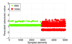
The main motivation for introducing the idea of hybrid-$(\ell_{1},\ell_{2})$ sampling on elements of ${\bm{\mathrm{A}}}$ comes from achieving a tighter bound on $s$ using a simple and intuitive probability distribution on elements of ${\bm{\mathrm{A}}}$. For this, we observe certain good properties of both $\ell_{1}$ and $\ell_{2}$ sampling for sparsification of noisy data (in practice, we experience data that are noisy, and it is perhaps impossible to separate “true” data from noise). We illustrate the behavior of $\ell_{1}$ and $\ell_{2}$ sampling on noisy data using the following synthetic example. We construct a $500\times 500$ binary data ${\bm{\mathrm{D}}}$ (Figure 1), and then perturb it by a random Gaussian matrix N whose elements $\textbf{N}_{ij}$ follow Gaussian distribution with mean zero and standard deviation $0.1$.

Figure 1: (left) Synthetic noiseless $500\times 500$ binary data ${\bm{\mathrm{D}}}$; (right) mesh view of noisy data ${\bm{\mathrm{A}}}_{0.1}$.

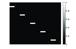
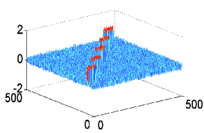
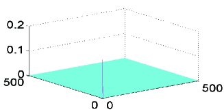
We denote this perturbed data matrix by ${\bm{\mathrm{A}}}_{0.1}$. First, we note that $\ell_{1}$ and $\ell_{2}$ sampling work identically on binary data ${\bm{\mathrm{D}}}$. However, Figure 2 depicts the change in behavior of $\ell_{1}$ and $\ell_{2}$ sampling sparsifying ${\bm{\mathrm{A}}}_{0.1}$. Data elements and noise in ${\bm{\mathrm{A}}}_{0.1}$ are the elements with non-zero and zero values in ${\bm{\mathrm{D}}}$, respectively. We sample $s=5000$ indices in i.i.d. trials according to $\ell_{1}$ and $\ell_{2}$ probabilities separately to produce sparse sketch $\tilde{{\bm{\mathrm{A}}}}$. Figure 2 shows that elements of $\tilde{{\bm{\mathrm{A}}}}$, produced by $\ell_{1}$ sampling, have controlled variance but most of them are noise. On the other hand, $\ell_{2}$ sampling is biased towards data elements, although small number of sampled noisy elements create large variance due to rescaling. Our hybrid-$(\ell_{1},\ell_{2})$ sampling benefits from this bias of $\ell_{2}$ towards data elements, as well as, regularization properties of $\ell_{1}$.

(a) $\ell_{1}$

(b) $\ell_{2}$

(c) Hybrid-$(\ell_{1},\ell_{2})$

Figure 2: Elements of sparse sketch $\tilde{{\bm{\mathrm{A}}}}$ produced from ${\bm{\mathrm{A}}}_{0.1}$ via (a) $\ell_{1}$ sampling, (b) $\ell_{2}$ sampling, and (c) hybrid-$(\ell_{1},\ell_{2})$ sampling with $\alpha=0.7$. The $y$-axis plots the rescaled absolute values (in $\ln$ scale) of $\tilde{{\bm{\mathrm{A}}}}$ corresponding to the sampled indices. $\ell_{1}$ sampling produces elements with controlled variance but it mostly samples noise, whereas $\ell_{2}$ samples a lot of data although producing large variance of rescaled elements. Hybrid-$(\ell_{1},\ell_{2})$ sampling uses $\ell_{1}$ as a regularizer while sampling a fairly large number of data that helps to preserve the structure of original data.

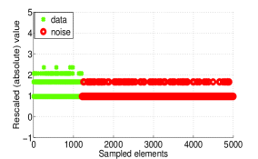
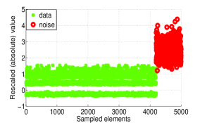
We parameterize our distribution using the variable $\alpha\in(0,1]$ that controls the balance between $\ell_{2}$ sampling and $\ell_{1}$ regularization. We derive an expression to compute $\alpha^{*}$, the optimal $\alpha$, corresponding to the smallest sample size that we need in order to achieve a given accuracy $\epsilon$ in (1). Setting $\alpha=1$, we reproduce the result of Achlioptas et al. (2013). However, $\alpha^{*}$ may be smaller than 1, and the bound on sample size $s$, using $\alpha^{*}$, is guaranteed to be tighter than that of Achlioptas et al. (2013).

2 Main Result

We present the quality-of-approximation result of our main algorithm (Algorithm 1). We define the sampling operator $\mathcal{S}_{\Omega}:\mathbb{R}^{m\times n}\rightarrow\mathbb{R}^{m\times n}$ in (3) that extracts elements from a given matrix ${\bm{\mathrm{A}}}\in\mathbb{R}^{m\times n}$. Let $\Omega$ be a multi-set of sampled indices $(i_{t},j_{t})$, for $t=1,...,s$. Then,

$$\mathcal{S}_{\Omega}\left({\bm{\mathrm{A}}}\right)={1\over s}\sum_{t=1}^{s}{{\bm{\mathrm{A}}}_{i_{t}j_{t}}\over p_{i_{t}j_{t}}}{\mathbf{e}}_{i_{t}}{\mathbf{e}}_{j_{t}}^{T},\quad(i_{t},j_{t})\in\Omega$$ (3)

Algorithm 1 randomly samples (in i.i.d. trials) $s$ elements of a given matrix ${\bm{\mathrm{A}}}$, according to a probability distribution $\{p_{ij}\}_{i,j=1}^{m,n}$ over the elements of ${\bm{\mathrm{A}}}$. Let the $p_{ij}$’s be as in eqn. (2). Then, we can prove the following theorem.

Theorem 1

Let ${\bm{\mathrm{A}}}\in\mathbb{R}^{m\times n}$ and let $\epsilon>0$ be an accuracy parameter. Let $\mathcal{S}_{\Omega}$ be the sampling operator defined in (3), and assume that the multi-set $\Omega$ is generated using sampling probabilities $\left\{p_{ij}\right\}_{i,j=1}^{m,n}$ as in (2). Then, with probability at least $1-\delta$,

$$\mbox{}\left\|\mathcal{S}_{\Omega}({\bm{\mathrm{A}}})-{\bm{\mathrm{A}}}\right\|_{2}\leq\epsilon\mbox{}\left\|{\bm{\mathrm{A}}}\right\|_{2},$$ (4)

if

$$s\geq{2\over\epsilon^{2}\mbox{}\left\|{\bm{\mathrm{A}}}\right\|_{2}^{2}}\left(\rho^{2}(\alpha)+\gamma(\alpha)\epsilon\mbox{}\left\|{\bm{\mathrm{A}}}\right\|_{2}/3\right)\ln\left({m+n\over\delta}\right)$$ (5)

where,

$$\xi_{ij}={\mbox{}\left\|{\bm{\mathrm{A}}}\right\|_{F}^{2}}/\left({\alpha\cdot\mbox{}\left\|{\bm{\mathrm{A}}}\right\|_{F}^{2}\over\left|{\bm{\mathrm{A}}}_{ij}\right|\cdot\mbox{}\left\|{\bm{\mathrm{A}}}\right\|_{1}}+(1-\alpha)\right),\text{ for }{\bm{\mathrm{A}}}_{ij}\neq 0,$$

$$\rho^{2}(\alpha)=\max\left\{\max_{i}\sum_{j=1}^{n}\xi_{ij},\max_{j}\sum_{i=1}^{m}\xi_{ij}\right\}-\sigma_{min}^{2}({\bm{\mathrm{A}}}),$$

$$\gamma(\alpha)=\max_{\stackrel{{\scriptstyle i,j:}}{{{\bm{\mathrm{A}}}_{ij}\neq 0}}}\left\{{\mbox{}\left\|{\bm{\mathrm{A}}}\right\|_{1}\over\alpha+(1-\alpha){\mbox{}\left\|{\bm{\mathrm{A}}}\right\|_{1}\cdot\left|{\bm{\mathrm{A}}}_{ij}\right|\over\mbox{}\left\|{\bm{\mathrm{A}}}\right\|_{F}^{2}}}\right\}+\mbox{}\left\|{\bm{\mathrm{A}}}\right\|_{2},$$

$\sigma_{min}({\bm{\mathrm{A}}})$ is the smallest singular value of ${\bm{\mathrm{A}}}$. Moreover, we can find $\alpha^{*}$ (optimal $\alpha$ corresponding to the smallest $s$) and $s^{*}$ (the smallest $s$), by solving the following optimization problem in (6):

$$\alpha^{*}=\min_{\alpha\in(0,1]}f(\alpha),\quad f(\alpha)=\rho^{2}(\alpha)+\gamma(\alpha)\epsilon\mbox{}\left\|{\bm{\mathrm{A}}}\right\|_{2}/3,$$ (6)

$$s^{*}={2\over\epsilon^{2}\mbox{}\left\|{\bm{\mathrm{A}}}\right\|_{2}^{2}}\left(\rho^{2}(\alpha^{*})+\gamma(\alpha^{*}){\epsilon\mbox{}\left\|{\bm{\mathrm{A}}}\right\|_{2}\over 3}\right)\ln\left({m+n\over\delta}\right)$$ (7)

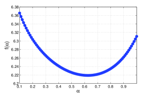
The functional form in (5) comes from the Matrix-Bernstein inequality in Lemma 1, with $\rho^{2}$ and $\gamma$ being functions of ${\bm{\mathrm{A}}}$ and $\alpha$. This gives us a flexibility to optimize the sample size with respect to $\alpha$ in (5), which is how we get the optimal $\alpha^{*}$. For a given matrix ${\bm{\mathrm{A}}}$, we can easily compute $\rho^{2}(\alpha)$ and $\gamma(\alpha)$ for various values of $\alpha$. Given an accuracy $\epsilon$ and failure probability $\delta$, we can compute $\alpha^{*}$ corresponding to the tightest bound on $s$. Note that, for $\alpha=1$ we reproduce the results of Achlioptas et al. (2013) (which was expressed using various matrix metrics). However, $\alpha^{*}$ may be smaller than 1, and is guaranteed to produce tighter $s$ comparing to extreme choices of $\alpha$ (e.g. $\alpha=1$ for $\ell_{1}$ sampling). We illustrate this by the plot in Figure 3.

Algorithm 1 Element-wise Matrix Sparsification

1:  Input: ${\bm{\mathrm{A}}}\in\mathbb{R}^{m\times n}$, accuracy parameter $\epsilon>0$.

2:  Set $s$ as in eq. (7).

3:  For $t=1\ldots s$ (i.i.d. trials with replacement) randomly sample pairs of indices $(i_{t},j_{t})\in[m]\times[n]$ with $\mathbb{P}\left[(i_{t},j_{t})=(i,j)\right]\ =\ p_{ij}$, where $p_{ij}$ are as in (2), using $\alpha$ as in (6).

4:  Output(sparse): $\mathcal{S}_{\Omega}\left({\bm{\mathrm{A}}}\right)={1\over s}\sum_{t=1}^{s}{{\bm{\mathrm{A}}}_{i_{t}j_{t}}\over p_{i_{t}j_{t}}}{\mathbf{e}}_{i_{t}}{\mathbf{e}}_{j_{t}}^{T}.$

Figure 3: Plot of $f(\alpha)$ in eqn (6) for data ${\bm{\mathrm{A}}}_{0.1}$. We use $\epsilon=0.05$ and $\delta=0.1$. $x$-axis plots $\alpha$ and $y$-axis is in log₁₀ scale. For this data, $\alpha^{*}\approx 0.6$.

We give a proof of Theorem 1 in Section 2.1.

2.1 Proof of Theorem 1

In this section we provide a proof of Theorem 1 following the proof outline of Drineas and Zouzias (2011); Achlioptas et al. (2013). We use the following non-commutative matrix-valued Bernstein bound of Recht (2011) as our main tool to prove Theorem 1. Using our notation we rephrase the matrix Bernstein bound.

Lemma 1

[Theorem 3.2 of Recht (2011)] Let ${\bm{\mathrm{M}}}_{1},{\bm{\mathrm{M}}}_{2},...,{\bm{\mathrm{M}}}_{s}$ be independent, zero-mean random matrices in $\mathbb{R}^{m\times n}$. Suppose

$$\max_{t\in[s]}\left\{\mbox{}\left\|\mathbb{E}({\bm{\mathrm{M}}}_{t}{\bm{\mathrm{M}}}_{t}^{T})\right\|_{2},\mbox{}\left\|\mathbb{E}({\bm{\mathrm{M}}}_{t}^{T}{\bm{\mathrm{M}}}_{t})\right\|_{2}\right\}\leq\rho^{2}$$

and $\mbox{}\left\|{\bm{\mathrm{M}}}_{t}\right\|_{2}\leq\gamma$ for all $t\in[s]$. Then, for any $\epsilon>0$,

$$\mbox{}\left\|{1\over s}\sum_{t=1}^{s}{\bm{\mathrm{M}}}_{t}\right\|_{2}\leq\epsilon$$

holds, subject to a failure probability at most

$$\left(m+n\right)\hbox{\rm exp}\left({-s\epsilon^{2}/2\over\rho^{2}+\gamma\epsilon/3}\right).$$

For all $t\in[s]$ we define the matrix ${\bm{\mathrm{M}}}_{t}\in\mathbb{R}^{m\times n}$ as follows:

$${\bm{\mathrm{M}}}_{t}={{\bm{\mathrm{A}}}_{i_{t}j_{t}}\over p_{i_{t}j_{t}}}{\mathbf{e}}_{i_{t}}{\mathbf{e}}_{j_{t}}^{T}-{\bm{\mathrm{A}}}.$$

It now follows that

$${1\over s}\sum_{t=1}^{s}{\bm{\mathrm{M}}}_{t}={1\over s}\sum_{t=1}^{s}\left[{{\bm{\mathrm{A}}}_{i_{t}j_{t}}\over p_{i_{t}j_{t}}}{\mathbf{e}}_{i_{t}}{\mathbf{e}}_{j_{t}}^{T}-{\bm{\mathrm{A}}}\right]=S_{\Omega}({\bm{\mathrm{A}}})-{\bm{\mathrm{A}}}.$$

We can bound $\mbox{}\left\|{\bm{\mathrm{M}}}_{t}\right\|_{2}$ for all $t\in[s]$. We define the following quantity:

$$\lambda={\mbox{}\left\|{\bm{\mathrm{A}}}\right\|_{1}\cdot\left|{\bm{\mathrm{A}}}_{ij}\right|\over\mbox{}\left\|{\bm{\mathrm{A}}}\right\|_{F}^{2}},\text{ for }{\bm{\mathrm{A}}}_{ij}\neq 0$$ (8)

Lemma 2

Using our notation, and using probabilities of the form (2), for all $t\in[s]$,

$$\mbox{}\left\|{\bm{\mathrm{M}}}_{t}\right\|_{2}\leq\max_{\stackrel{{\scriptstyle i,j:}}{{{\bm{\mathrm{A}}}_{ij}\neq 0}}}{\mbox{}\left\|{\bm{\mathrm{A}}}\right\|_{1}\over\alpha+(1-\alpha)\lambda}+\mbox{}\left\|{\bm{\mathrm{A}}}\right\|_{2}.$$

Proof: Using probabilities of the form (2), and because ${\bm{\mathrm{A}}}_{ij}=0$ is never sampled,

$$\mbox{}\left\|{\bm{\mathrm{M}}}_{t}\right\|_{2}=\mbox{}\left\|{{\bm{\mathrm{A}}}_{i_{t}j_{t}}\over p_{i_{t}j_{t}}}{\mathbf{e}}_{i_{t}}{\mathbf{e}}_{j_{t}}^{T}-{\bm{\mathrm{A}}}\right\|_{2}\leq\max_{\stackrel{{\scriptstyle i,j:}}{{{\bm{\mathrm{A}}}_{ij}\neq 0}}}\left\{\left({\alpha\over\mbox{}\left\|{\bm{\mathrm{A}}}\right\|_{1}}+{(1-\alpha)\cdot\left|{\bm{\mathrm{A}}}_{ij}\right|\over\mbox{}\left\|{\bm{\mathrm{A}}}\right\|_{F}^{2}}\right)^{-1}\right\}+\mbox{}\left\|{\bm{\mathrm{A}}}\right\|_{2}$$

Using (8), we obtain the bound.
$\diamond$
Next we bound the spectral norm of the expectation of ${\bm{\mathrm{M}}}_{t}{\bm{\mathrm{M}}}_{t}^{T}$.

Lemma 3

Using our notation, and using probabilities of the form (2), for all $t\in[s]$,

$$\mbox{}\left\|\mathbb{E}({\bm{\mathrm{M}}}_{t}{\bm{\mathrm{M}}}_{t}^{T})\right\|_{2}\leq\mbox{}\left\|{\bm{\mathrm{A}}}\right\|_{F}^{2}\beta_{1}-\sigma_{min}^{2}({\bm{\mathrm{A}}}),$$

where,

$$\beta_{1}=\max_{i}\sum_{j=1}^{n}\left({\alpha\cdot\mbox{}\left\|{\bm{\mathrm{A}}}\right\|_{F}^{2}\over\left|{\bm{\mathrm{A}}}_{ij}\right|\cdot\mbox{}\left\|{\bm{\mathrm{A}}}\right\|_{1}}+(1-\alpha)\right)^{-1},\text{ for }{\bm{\mathrm{A}}}_{ij}\neq 0.$$

Proof: Recall that ${\bm{\mathrm{A}}}=\sum_{i,j=1}^{m,n}{\bm{\mathrm{A}}}_{ij}{\mathbf{e}}_{i}{\mathbf{e}}_{j}^{T}$ and ${\bm{\mathrm{M}}}_{t}={{\bm{\mathrm{A}}}_{i_{t}j_{t}}\over p_{i_{t}j_{t}}}{\mathbf{e}}_{i_{t}}{\mathbf{e}}_{j_{t}}^{T}-{\bm{\mathrm{A}}}$ to derive

$$\mathbb{E}[{\bm{\mathrm{M}}}_{t}{\bm{\mathrm{M}}}_{t}^{T}] = \sum_{i,j=1}^{m,n}p_{ij}\left({{\bm{\mathrm{A}}}_{ij}\over p_{ij}}{\mathbf{e}}_{i}{\mathbf{e}}_{j}^{T}-{\bm{\mathrm{A}}}\right)\left({{\bm{\mathrm{A}}}_{ij}\over p_{ij}}{\mathbf{e}}_{j}{\mathbf{e}}_{i}^{T}-{\bm{\mathrm{A}}}^{T}\right)$$

$$= \sum_{i,j=1}^{m,n}\left({{\bm{\mathrm{A}}}_{ij}^{2}\over p_{ij}}{\mathbf{e}}_{i}{\mathbf{e}}_{i}^{T}\right)-{\bm{\mathrm{A}}}{\bm{\mathrm{A}}}^{T}.$$

Sampling according to probabilities of eqn. (2), and because ${\bm{\mathrm{A}}}_{ij}=0$ is never sampled, we get, for ${\bm{\mathrm{A}}}_{ij}\neq 0$,

$$\sum_{i,j=1}^{m,n}{{\bm{\mathrm{A}}}_{ij}^{2}\over p_{ij}} = \mbox{}\left\|{\bm{\mathrm{A}}}\right\|_{F}^{2}\sum_{i,j=1}^{m,n}\left({\alpha\cdot\mbox{}\left\|{\bm{\mathrm{A}}}\right\|_{F}^{2}\over\left|{\bm{\mathrm{A}}}_{ij}\right|\cdot\mbox{}\left\|{\bm{\mathrm{A}}}\right\|_{1}}+(1-\alpha)\right)^{-1},$$

$$\leq \mbox{}\left\|{\bm{\mathrm{A}}}\right\|_{F}^{2}\sum_{i=1}^{m}\max_{i}\sum_{j=1}^{n}\left({\alpha\cdot\mbox{}\left\|{\bm{\mathrm{A}}}\right\|_{F}^{2}\over\left|{\bm{\mathrm{A}}}_{ij}\right|\cdot\mbox{}\left\|{\bm{\mathrm{A}}}\right\|_{1}}+(1-\alpha)\right)^{-1}.$$

Thus,

$$\mathbb{E}[{\bm{\mathrm{M}}}_{t}{\bm{\mathrm{M}}}_{t}^{T}]\preceq\mbox{}\left\|{\bm{\mathrm{A}}}\right\|_{F}^{2}\beta_{1}\sum_{i=1}^{m}{\mathbf{e}}_{i}{\mathbf{e}}_{i}^{T}-{\bm{\mathrm{A}}}{\bm{\mathrm{A}}}^{T}=\mbox{}\left\|{\bm{\mathrm{A}}}\right\|_{F}^{2}\beta_{1}{\bm{\mathrm{I}}}_{m}-{\bm{\mathrm{A}}}{\bm{\mathrm{A}}}^{T}.$$

Note that, $\mbox{}\left\|{\bm{\mathrm{A}}}\right\|_{F}^{2}\beta_{1}{\bm{\mathrm{I}}}_{m}$ is a diagonal matrix with all entries non-negative, and ${\bm{\mathrm{A}}}{\bm{\mathrm{A}}}^{T}$ is a postive semi-definite matrix. Therefore,

$$\mbox{}\left\|\mathbb{E}[{\bm{\mathrm{M}}}_{t}{\bm{\mathrm{M}}}_{t}^{T}]\right\|_{2}\leq\mbox{}\left\|{\bm{\mathrm{A}}}\right\|_{F}^{2}\beta_{1}-\sigma_{min}^{2}({\bm{\mathrm{A}}}).$$

$\diamond$
Similarly, we can obtain

$$\mbox{}\left\|\mathbb{E}[{\bm{\mathrm{M}}}_{t}^{T}{\bm{\mathrm{M}}}_{t}]\right\|_{2}\leq\mbox{}\left\|{\bm{\mathrm{A}}}\right\|_{F}^{2}\beta_{2}-\sigma_{min}^{2}({\bm{\mathrm{A}}}),$$

where,

$$\beta_{2}=\max_{j}\sum_{i=1}^{m}\left({\alpha\cdot\mbox{}\left\|{\bm{\mathrm{A}}}\right\|_{F}^{2}\over\left|{\bm{\mathrm{A}}}_{ij}\right|\cdot\mbox{}\left\|{\bm{\mathrm{A}}}\right\|_{1}}+(1-\alpha)\right)^{-1},\text{ for }{\bm{\mathrm{A}}}_{ij}\neq 0.$$

We can now apply Theorem 1 with

$$\rho^{2}(\alpha)=\mbox{}\left\|{\bm{\mathrm{A}}}\right\|_{F}^{2}\max\{\beta_{1},\beta_{2}\}-\sigma_{min}^{2}({\bm{\mathrm{A}}})$$

and

$$\gamma(\alpha)={\mbox{}\left\|{\bm{\mathrm{A}}}\right\|_{1}\over\alpha+(1-\alpha)\lambda}+\mbox{}\left\|{\bm{\mathrm{A}}}\right\|_{2}$$

to conclude that $\mbox{}\left\|\mathcal{S}_{\Omega}({\bm{\mathrm{A}}})-{\bm{\mathrm{A}}}\right\|_{2}\leq\varepsilon$ holds subject to a failure probability at most

$$\left(m+n\right)\hbox{\rm exp}\left({(-s\varepsilon^{2}/2)}/{\left(\rho^{2}(\alpha)+\gamma(\alpha)\varepsilon/3\right)}\right).$$

Bounding the failure probability by $\delta$, and setting $\varepsilon=\epsilon\cdot\mbox{}\left\|{\bm{\mathrm{A}}}\right\|_{2},$ we complete the proof.

3 One-pass Hybrid-$(\ell_{1},\ell_{2})$ Sampling

Here we discuss the implementation of $(\ell_{1},\ell_{2})$-hybrid sampling in one pass over the input matrix ${\bm{\mathrm{A}}}$ using $O(s)$ memory, that is, a streaming model. We know that both $\ell_{1}$ and $\ell_{2}$ sampling can be done in one pass using $O(s)$ memory (see Algorithm SELECT p. 137 of Drineas et al. (2006) ). In our hybrid sampling, we want parameter $\alpha$ to depend on data elements, i.e., we do not want to ‘fix’ it prior to the arrival of data stream. Here we give an algorithm (Algorithm 2) to implement a one-pass version of the hybrid sampling without knowing $\alpha$ a priori.

Algorithm 2 One-pass hybrid-$(\ell_{1},\ell_{2})$ sampling

1:  Input: ${\bm{\mathrm{A}}}_{ij}$ for all $(i,j)\in[m]\times[n]$, arbitrarily ordered, and sample size $s$.

2:  Apply SELECT algorithm in parallel with $O(s)$ memory using $\ell_{1}$ probabilities to sample $s$ independent indices $(i_{t_{1}},j_{t_{1}})$ and corresponding elements ${\bm{\mathrm{A}}}_{i_{t_{1}}j_{t_{1}}}$ to form random multiset $S_{1}$ of triples $(i_{t_{1}},j_{t_{1}},{\bm{\mathrm{A}}}_{i_{t_{1}}j_{t_{1}}})$, for $t_{1}=1,...,s$.

3:  Run step 2 in parallel to form another independent multiset $S_{3}$ of triples $(i_{t_{3}},j_{t_{3}},{\bm{\mathrm{A}}}_{i_{t_{3}}j_{t_{3}}})$, for $t_{3}=1,...,s$. (This step is only for Algorithm 3)

4:  Apply SELECT algorithm in parallel with $O(s)$ memory using $\ell_{2}$ probabilities to sample $s$ independent indices $(i_{t_{2}},j_{t_{2}})$ and corresponding elements ${\bm{\mathrm{A}}}_{i_{t_{2}}j_{t_{2}}}$ to form random multiset $S_{1}$ of triples $(i_{t_{2}},j_{t_{2}},{\bm{\mathrm{A}}}_{i_{t_{2}}j_{t_{2}}})$, for $t_{2}=1,...,s$.

5:  Run step 4 in parallel to form another independent multiset $S_{4}$ of triples $(i_{t_{4}},j_{t_{4}},{\bm{\mathrm{A}}}_{i_{t_{4}}j_{t_{4}}})$, for $t_{4}=1,...,s$. (This step is only for Algorithm 3)

6:  Compute and store $\mbox{}\left\|{\bm{\mathrm{A}}}\right\|_{F}^{2}$ and $\mbox{}\left\|{\bm{\mathrm{A}}}\right\|_{1}$ in parallel.

7:  Set the value of $\alpha\in(0,1]$ (using Algorithm 3).

8:  Create empty multiset of triples $S$.

9:  ${\bm{\mathrm{X}}}\leftarrow\textbf{0}_{m\times n}$.

10:  For $t=1\ldots s$

11:   Generate a uniform random number $x\in[0,1]$.

12:   if $x\geq\alpha$, $S(t)\leftarrow S_{1}(t)$; otherwise, $S(t)\leftarrow S_{2}(t)$.

13:   $(i_{t},j_{t})\leftarrow S(t,1:2)$.

14:   $p\leftarrow\alpha\cdot{\left|S(t,3)\right|\over\mbox{}\left\|{\bm{\mathrm{A}}}\right\|_{1}}+(1-\alpha)\cdot{\left|S(t,3)\right|^{2}\over\mbox{}\left\|{\bm{\mathrm{A}}}\right\|_{F}^{2}}$

15:   ${\bm{\mathrm{X}}}\leftarrow{\bm{\mathrm{X}}}+{S(t,3)\over p\cdot s}e_{i_{t}}e_{j_{t}}^{T}$.

16:  End

17:  Output: random multiset $S$, and sparse matrix ${\bm{\mathrm{X}}}$.

We note that steps 2-5 of Algorithm 2 access the elements of ${\bm{\mathrm{A}}}$ only once, in parallel, to form independent multisets $S_{1}$, $S_{2}$, $S_{3}$, and $S_{4}$. Step 6 computes $\mbox{}\left\|{\bm{\mathrm{A}}}\right\|_{F}^{2}$ and $\mbox{}\left\|{\bm{\mathrm{A}}}\right\|_{1}$ in parallel in one pass over ${\bm{\mathrm{A}}}$. Subsequent steps do not need to access ${\bm{\mathrm{A}}}$ anymore. Interestingly, we set $\alpha$ in step 7 when the data stream is gone. Steps 10-16 sample $s$ elements from $S_{1}$ and $S_{2}$ based on the $\alpha$ in step 7, and produce sparse matrix ${\bm{\mathrm{X}}}$ based on the sampled entries in random multiset $S$. Theorem 2 shows that Algorithm 2 indeed samples elements from ${\bm{\mathrm{A}}}$ according to the hybrid-$(\ell_{1},\ell_{2})$ probabilities in eqn (2).

Theorem 2

Using the notations in Algorithm 2, for $\alpha\in(0,1]$, $t=1,...,s$,

$${P\left[{S(t)=(i,j,{\bm{\mathrm{A}}}_{ij})}\right]}=\alpha\cdot p_{1}+(1-\alpha)\cdot p_{2},$$

where  $p_{1}={\left|{\bm{\mathrm{A}}}_{ij}\right|\over\mbox{}\left\|{\bm{\mathrm{A}}}\right\|_{1}}$  and  $p_{2}={{\bm{\mathrm{A}}}_{ij}^{2}\over\mbox{}\left\|{\bm{\mathrm{A}}}\right\|_{F}^{2}}$.

Proof: Here we use the notations in Theorem 2. Note that $t$-th elements of $S_{1}$ and $S_{2}$ are sampled independently with $\ell_{1}$ and $\ell_{2}$ probabilities, respectively. We consider the following disjoint events:

$$\mathcal{E}_{1}:S_{1}(t)=(i,j,{\bm{\mathrm{A}}}_{ij})\land S_{2}(t)\neq(i,j,{\bm{\mathrm{A}}}_{ij})$$

$$\mathcal{E}_{2}:S_{1}(t)\neq(i,j,{\bm{\mathrm{A}}}_{ij})\land S_{2}(t)=(i,j,{\bm{\mathrm{A}}}_{ij})$$

$$\mathcal{E}_{3}:S_{1}(t)=(i,j,{\bm{\mathrm{A}}}_{ij})\land S_{2}(t)=(i,j,{\bm{\mathrm{A}}}_{ij})$$

$$\mathcal{E}_{4}:S_{1}(t)\neq(i,j,{\bm{\mathrm{A}}}_{ij})\land S_{2}(t)\neq(i,j,{\bm{\mathrm{A}}}_{ij})$$

Let us denote the events $x_{1}:x\geq\alpha$ and $x_{2}:x<\alpha$. Clearly, ${P\left[{x_{1}}\right]}=\alpha,{P\left[{x_{2}}\right]}=1-\alpha$. Since the elements $S_{1}(t)$ and $S_{2}(t)$ are sampled independently, we have

$${P\left[{\mathcal{E}_{1}}\right]} = {P\left[{S_{1}(t)=(i,j,{\bm{\mathrm{A}}}_{ij})}\right]}{P\left[{S_{2}(t)\neq(i,j,{\bm{\mathrm{A}}}_{ij})}\right]}=p_{1}(1-p_{2})$$

$${P\left[{\mathcal{E}_{2}}\right]} = (1-p_{1})p_{2}$$

$${P\left[{\mathcal{E}_{3}}\right]} = p_{1}p_{2}$$

$${P\left[{\mathcal{E}_{4}}\right]} = (1-p_{1})(1-p_{2})$$

We note that $\alpha$ may be dependent on the elements of $S_{3}$ and $S_{4}$ (in Algorithm 3), but is independent of elements of $S_{1}$ and $S_{2}$. Therefore, events $x_{1}$ and $x_{2}$ are independent of the events $\mathcal{E}_{j}$, $j=1,2,3,4$. Thus,

$${P\left[{S(t)=(i,j,{\bm{\mathrm{A}}}_{ij})}\right]}$$

$$= {P\left[{(\mathcal{E}_{1}\land x_{1})\lor(\mathcal{E}_{2}\land x_{2})\lor\mathcal{E}_{3}}\right]}$$

$$= {P\left[{\mathcal{E}_{1}\land x_{1}}\right]}+{P\left[{\mathcal{E}_{2}\land x_{2}}\right]}+{P\left[{\mathcal{E}_{3}}\right]}$$

$$= {P\left[{\mathcal{E}_{1}}\right]}{P\left[{x_{1}}\right]}+{P\left[{\mathcal{E}_{2}}\right]}{P\left[{x_{2}}\right]}+{P\left[{\mathcal{E}_{3}}\right]}$$

$$= p_{1}(1-p_{2})\alpha+(1-p_{1})p_{2}(1-\alpha)+p_{1}p_{2}$$

$$= \alpha\cdot p_{1}+(1-\alpha)\cdot p_{2}$$

$\diamond$

Note that, Theorem 2 holds for any arbitrary $\alpha\in(0,1]$ in line 7 of Algorithm 2, i.e., Algorithm 3 is not essential for correctness of Theorem 2. We only need $\alpha$ to be independent of elements of $S_{1}$ and $S_{2}$. However, we use Algorithm 3 to get an iterative estimate of $\alpha^{*}$ (Section 3.1) in one pass over ${\bm{\mathrm{A}}}$. In this case, we need additional independent multisets $S_{3}$ and $S_{4}$ to ‘learn’ the parameter $\alpha^{*}$. Algorithm 2 (without Algorithm 3) requires a memory twice as large required by $\ell_{1}$ or $\ell_{2}$ sampling. Using Algorithm 3 this requirement is four times as large. However, in both the cases the asymptotic memory requirement remains the same $O(s)$.

3.1 Iterative Estimate of $\alpha^{*}$

We obtain independent random multiset of triples $S_{3}$ and $S_{4}$, each containing $s$ elements from ${\bm{\mathrm{A}}}$ in one pass, in Algorithm 2. We can create a sparse random matrix ${\bm{\mathrm{X}}}$, as shown in step 11 in Algorithm 3, that is an unbiased estimator of ${\bm{\mathrm{A}}}$. We use this ${\bm{\mathrm{X}}}$ as a proxy for ${\bm{\mathrm{A}}}$ to estimate the quantities we need in order to solve the optimization problem in (9).

Algorithm 3 Iterative estimate of $\alpha^{*}$

1:  Input: Multiset of triples $S_{3}$ and $S_{4}$ with $s$ elements each, number of iteration $\tau$, accuracy $\epsilon$, $\mbox{}\left\|{\bm{\mathrm{A}}}\right\|_{F}^{2}$, and $\mbox{}\left\|{\bm{\mathrm{A}}}\right\|_{1}$.

2:  Create empty multiset of triples $S$.

3:  $\alpha_{0}=0.5$

4:  For $k=1\ldots\tau$

5:   ${\bm{\mathrm{X}}}\leftarrow\textbf{0}_{m\times n}$.

6:   For $t=1\ldots s$

7:    Generate a uniform random number $x\in[0,1]$.

8:    If $x\geq\alpha_{k-1}$, $S(t)\leftarrow S_{3}(t)$; else, $S(t)\leftarrow S_{4}(t)$.

9:    $(i_{t},j_{t})\leftarrow S(t,1:2)$.

10:    $p\leftarrow\alpha_{k-1}\cdot{\left|S(t,3)\right|\over\mbox{}\left\|{\bm{\mathrm{A}}}\right\|_{1}}+(1-\alpha_{k-1})\cdot{\left|S(t,3)\right|^{2}\over\mbox{}\left\|{\bm{\mathrm{A}}}\right\|_{F}^{2}}$

11:    ${\bm{\mathrm{X}}}\leftarrow{\bm{\mathrm{X}}}+{S(t,3)\over p\cdot s}e_{i_{t}}e_{j_{t}}^{T}$.

12:   End

13:   $\alpha_{k}\leftarrow$ $\tilde{\alpha}$ in (9) using ${\bm{\mathrm{X}}}$.

14:  End

15:  Output: $\alpha_{\tau}$.

$$\tilde{\alpha}:\min_{\alpha\in(0,1]}\left\{\left(\tilde{\rho}^{2}(\alpha)+\tilde{\gamma}(\alpha)\epsilon\mbox{}\left\|{\bm{\mathrm{X}}}\right\|_{2}/3\right)\right\}$$ (9)

where, for all $(i,j)\in S(:,1:2)$

$$\tilde{\xi}_{ij}={\mbox{}\left\|{\bm{\mathrm{X}}}\right\|_{F}^{2}}/\left({\alpha\cdot\mbox{}\left\|{\bm{\mathrm{X}}}\right\|_{F}^{2}\over\left|{\bm{\mathrm{X}}}_{ij}\right|\cdot\mbox{}\left\|{\bm{\mathrm{X}}}\right\|_{1}}+(1-\alpha)\right),$$

$$\tilde{\rho}^{2}(\alpha)=\max\left\{\max_{i}\sum_{j=1}^{n}\tilde{\xi}_{ij},\max_{j}\sum_{i=1}^{m}\tilde{\xi}_{ij}\right\},$$

$$\tilde{\gamma}(\alpha)=\max_{ij}\left\{{\mbox{}\left\|{\bm{\mathrm{X}}}\right\|_{1}\over\alpha+(1-\alpha){\mbox{}\left\|{\bm{\mathrm{X}}}\right\|_{1}\cdot\left|{\bm{\mathrm{X}}}_{ij}\right|\over\mbox{}\left\|{\bm{\mathrm{X}}}\right\|_{F}^{2}}}\right\}+\mbox{}\left\|{\bm{\mathrm{X}}}\right\|_{F}.$$

We note that $\mbox{}\left\|{\bm{\mathrm{X}}}\right\|_{0}\leq s$. We can compute the quantities $\tilde{\rho}(\alpha)$ and $\tilde{\gamma}(\alpha)$, for a fixed $\alpha$, using $O(s)$ memory. We consider $\varepsilon=\epsilon\cdot\mbox{}\left\|{\bm{\mathrm{X}}}\right\|_{2}$ to be the given accuracy.

4 Fast Approximation of PCA

Here, we discuss a provable algorithm (Algorithm 4) to speed up computation of PCA applying element-wise sampling. We sparsify a given centered data ${\bm{\mathrm{A}}}$ to produce a sparse unbiased estimator $\tilde{{\bm{\mathrm{A}}}}$ by sampling $s$ elements in i.i.d. trials according to our hybrid-$(\ell_{1},\ell_{2})$ distribution in (2). Computation of rank-truncated SVD on sparse data is fast, and we consider the right singular vectors of $\tilde{{\bm{\mathrm{A}}}}$ as the approximate principal components of ${\bm{\mathrm{A}}}$. Naturally, more samples produce better approximation. However, this reduces sparsity, and consequently we lose the speed advantage.

Algorithm 4 Fast Approximation of PCA

1:  Input: Centered data ${\bm{\mathrm{A}}}\in\mathbb{R}^{m\times n}$, sparsity parameter $s>0$, and rank parameter $k$.

2:  Produce sparse unbiased estimator $\tilde{{\bm{\mathrm{A}}}}$ from ${\bm{\mathrm{A}}}$, in $s$ i.i.d. trials using Algorithm 1.

3:  Perform rank truncated SVD on sparse matrix $\tilde{{\bm{\mathrm{A}}}}$, i.e., $[\tilde{{\bm{\mathrm{U}}}}_{k},\tilde{{\bm{\mathrm{D}}}}_{k},\tilde{{\bm{\mathrm{V}}}}_{k}]$ = SVD($\tilde{{\bm{\mathrm{A}}}}$, $k$).

4:  Output: $\tilde{{\bm{\mathrm{V}}}}_{k}$ (columns of $\tilde{{\bm{\mathrm{V}}}}_{k}$ are the ordered PCA’s).

Theorem 3 shows the quality of approximation of principal components produced by Algorithm 4.

Theorem 3

Let ${\bm{\mathrm{A}}}\in\mathbb{R}^{m\times n}$ be a given matrix, and $\tilde{{\bm{\mathrm{A}}}}$ be a sparse sketch produced by Algorithm 1. Let $\tilde{{\bm{\mathrm{V}}}}_{k}$ be the PCA’s of $\tilde{{\bm{\mathrm{A}}}}$ computed in step 3 of Algorithm 4. Then

$$\mbox{}\left\|{\bm{\mathrm{A}}}-{\bm{\mathrm{A}}}\tilde{{\bm{\mathrm{V}}}}_{k}\tilde{{\bm{\mathrm{V}}}}_{k}^{T}\right\|_{F}^{2} \leq \mbox{}\left\|{\bm{\mathrm{A}}}-{\bm{\mathrm{A}}}_{k}\right\|_{F}^{2}+{4\mbox{}\left\|{\bm{\mathrm{A}}}_{k}\right\|_{F}^{2}\over\sigma_{k}({\bm{\mathrm{A}}})}\mbox{}\left\|{\bm{\mathrm{A}}}-\tilde{{\bm{\mathrm{A}}}}\right\|_{2}$$

$$\mbox{}\left\|{\bm{\mathrm{A}}}_{k}-\tilde{{\bm{\mathrm{A}}}}_{k}\right\|_{F} \leq \sqrt{8k}\cdot\left(\mbox{}\left\|{\bm{\mathrm{A}}}-{{\bm{\mathrm{A}}}}_{k}\right\|_{2}+\mbox{}\left\|{\bm{\mathrm{A}}}-\tilde{{\bm{\mathrm{A}}}}\right\|_{2}\right)$$

$$\mbox{}\left\|{\bm{\mathrm{A}}}-\tilde{{\bm{\mathrm{A}}}}_{k}\right\|_{F} \leq \mbox{}\left\|{\bm{\mathrm{A}}}-{{\bm{\mathrm{A}}}}_{k}\right\|_{F}+\sqrt{8k}\cdot\left(\mbox{}\left\|{\bm{\mathrm{A}}}-{{\bm{\mathrm{A}}}}_{k}\right\|_{2}+\mbox{}\left\|{\bm{\mathrm{A}}}-\tilde{{\bm{\mathrm{A}}}}\right\|_{2}\right)$$

The first inequality of Theorem 3 bounds the approximation of projected data onto the space spanned by top $k$ approximate PCA’s. The second and third inequalities measure the quality of $\tilde{{\bm{\mathrm{A}}}}_{k}$ as a surrogate for ${\bm{\mathrm{A}}}_{k}$ and the quality of projection of sparsified data onto approximate PCA’s, respectively.

Proofs of first two inequalities of Theorem 3 follow from Theorem 5 and Theorem 8 of Achlioptas and McSherry (2001), respectively. The last inequality follows from the triangle inequality. The last two inequalities above are particularly useful in cases where ${\bm{\mathrm{A}}}$ is inherently low-rank and we choose an appropriate $k$ for approximation, for which $\mbox{}\|{\bm{\mathrm{A}}}-{\bm{\mathrm{A}}}_{k}\|_{2}$ is small.

5 Experiments

In this section we perform various element-wise sampling experiments on synthetic and real data to show how well the sparse sketches preserve the structure of the original data, in spectral norm. Also, we show results on the quality of the PCA’s derived from sparse sketches.

5.1 Algorithms for Sparse Sketches

We use Algorithm 1 as a prototypical algorithm to produce sparse sketches from a given matrix via various sampling methods. Note that, we can plug-in any element-wise probability distribution in Algorithm 1 to produce (unbiased) sparse matrices. We construct sparse sketches via our optimal hybrid-($\ell_{1},\ell_{2}$) sampling, along with other sampling methods related to extreme choices of $\alpha$, such as, $\ell_{1}$ sampling for $\alpha=1$. Also, we use element-wise leverage scores (Chen et al. (2014)) for sparsification of low-rank data. Element-wise leverage scores are used in the context of low-rank matrix completion by Chen et al. (2014). Let ${\bm{\mathrm{A}}}$ be a $m\times n$ matrix of rank $\rho$, and its SVD if given by ${\bm{\mathrm{A}}}={\bm{\mathrm{U}}}{\bm{\mathrm{\Sigma}}}{\bm{\mathrm{V}}}^{T}$. Then, we define $\mu_{i}$ (row leverage scores), $\nu_{j}$ (column leverage scores), and element-wise leverage scores $p_{lev}$ as follows:

$$\mu_{i}=\mbox{}\left\|{\bm{\mathrm{U}}}_{(i)}\right\|_{2}^{2},\quad\nu_{j}=\mbox{}\left\|{\bm{\mathrm{V}}}_{(j)}\right\|_{2}^{2},\quad p_{lev}={\mu_{i}+\nu_{j}\over(m+n)\rho},\quad i\in[m],j\in[n]$$

Note that $p_{lev}$ is a probability distribution on the elements of ${\bm{\mathrm{A}}}$. Leverage scores become uniform if the matrix ${\bm{\mathrm{A}}}$ is full rank. We use $p_{lev}$ in Algorithm 1 to produce sparse sketch $\tilde{{\bm{\mathrm{A}}}}$ of a low-rank data ${\bm{\mathrm{A}}}$.

5.1.1 Experimental Design for Sparse Sketches

We compute the theoretical optimal mixing parameter $\alpha^{*}$ by solving eqn (6) for various datasets. We compare this $\alpha^{*}$ with the theoretical condition derived by Achlioptas et al. (2013) (for cases when $\ell_{1}$ sampling outperforms $\ell_{2}$ sampling). We verify the accuracy of $\alpha^{*}$ by measuring the quality of the sparse sketches $\tilde{{\bm{\mathrm{A}}}}$, $\mathcal{E}=\mbox{}\|{\bm{\mathrm{A}}}-\tilde{{\bm{\mathrm{A}}}}\|_{2}/\mbox{}\|{\bm{\mathrm{A}}}\|_{2}$ for various sampling distributions. Let $\mathcal{E}_{h}$, $\mathcal{E}_{1}$, and $\mathcal{E}_{lev}$ denote the quality of sparse sketches produced via optimal hybrid sampling, $\ell_{1}$ sampling, and element-wise leverage scores $p_{lev}$, respectively. We compare $\mathcal{E}_{h}$, $\mathcal{E}_{1}$, and $\mathcal{E}_{lev}$ for various sample sizes for real and synthetic datasets.

5.2 Algorithms for Fast PCA

We compare three algorithms for computing PCA of the centered data. Let the actual PCA of the original data be $\mathcal{A}$. We use Algorithm 4 to compute approximate PCA via our optimal hybrid-$(\ell_{1},\ell_{2})$ sampling. Let us denote this approximate PCA by $\mathcal{H}$. Also, we compute PCA of a Gaussian random projection of the original data to compare the quality of $\mathcal{H}$. Let ${\bm{\mathrm{A}}}_{G}={\bm{\mathrm{G}}}{\bm{\mathrm{A}}}\in\mathbb{R}^{r\times n}$, where ${\bm{\mathrm{A}}}\in\mathbb{R}^{m\times n}$ is the original data, and ${\bm{\mathrm{G}}}$ is a $r\times m$ standard Gaussian matrix. Let the PCA of this random projection ${\bm{\mathrm{A}}}_{G}$ be $\mathcal{G}$. Also, let $T_{a}$, $T_{h}$, and $T_{G}$ be the computation time (in milliseconds) for $\mathcal{A}$, $\mathcal{H}$, and $\mathcal{G}$, respectively.

5.2.1 Experimental Design for Fast PCA

We compare the visual quality of $\mathcal{A}$, $\mathcal{H}$, and $\mathcal{G}$ for image datasets. Also, we compare the computation time $T_{a}$, $T_{h}$, and $T_{G}$ for these datasets.

5.3 Description of Data

In this section we describe the synthetic and real datasets we use in our experiments.

5.3.1 Synthetic Data

We construct a binary $500\times 500$ image data ${\bm{\mathrm{D}}}$ (see Figure 1). We add random noise to perturb the elements of the ‘pure’ data ${\bm{\mathrm{D}}}$. Specifically, we construct a $500\times 500$ noise matrix N whose elements $\textbf{N}_{ij}$ are drawn i.i.d from Gaussian with mean zero and standard deviation $\sigma$. We use two different values for $\sigma$ in our experiments: $\sigma=0.05$ and $\sigma=0.10$. For each $\sigma$, we note the following ratios:

$$\text{Noise-to-signal energy ratio}={\mbox{}\left\|\textbf{N}\right\|_{F}}/{\mbox{}\left\|{\bm{\mathrm{D}}}\right\|_{F}},$$

$$\text{ Spectral ratio}={\mbox{}\left\|\textbf{N}\right\|_{2}}/{\sigma_{k}({\bm{\mathrm{D}}})},$$

where $\sigma_{k}({\bm{\mathrm{D}}})$ is the $k$-th largest singular value of ${\bm{\mathrm{D}}}$. For $\sigma=0.05$ and $\sigma=0.10$, average Noise-to-signal energy ratio are $0.44$ and $0.88$, average Spectral ratio are $0.09$ and $0.17$, and average maximum absolute values of noise turn out to be $0.25$ and $0.50$, respectively. We denote noisy data by ${\bm{\mathrm{A}}}_{0.05}$ (respectively ${\bm{\mathrm{A}}}_{0.1}$) when ${\bm{\mathrm{D}}}$ is perturbed by N whose elements $\textbf{N}_{ij}$ are drawn i.i.d from a Gaussian distribution with mean zero and $\sigma=0.05$ (respectively $\sigma=0.1$).

5.3.2 TechTC Datasets

These datasets (Gabrilovich and Markovitch (2004)) are bag-of-words features for document-term data describing two topics (ids). We choose four such datasets: TechTC1 with ids 10567 and 11346, TechTC2 with ids 10567 and 12121, TechTC3 with ids 11498 and 14517, TechTC4 with ids 11346 and 22294. Rows represent documents and columns are the words. We preprocessed the data by removing all the words of length four or smaller, and then normalized the rows by dividing each row by its Frobenius norm. The following table lists the dimension of the TechTC datasets.

Dimension ($m\times n)$	$m$	$n$
TechTC1	139	15170
TechTC2	138	11859
TechTC3	125	15485
TechTC4	125	14392

Table 1: Dimension of TechTC datasets

5.3.3 Handwritten Digit Data

A dataset (Hull (1994)) of three handwritten digits: six (664 samples), nine (644 samples), and one (1005 samples). Pixels are treated as features, and pixel values are normalized in [-1,1]. Each $16\times 16$ digit image is first represented by a column vector by appending the pixels column-wise. Then, we use the transpose of this column vector to form a row in the data matrix. The number of rows $m=2313$, and columns $n=256$.

5.3.4 Stock Data

We use a stock market dataset (S&P) containing prices of 1218 stocks collected between 1983 and 2011. This temporal dataset has 7056 snapshots of stock prices. Thus, we have $m=1218$ and $n=7056$.

We provide summary statistics for all the datasets in Table 2. In order to compare our results with Achlioptas et al. (2013) we review the matrix metrics that they use. Let the numeric density of matrix ${\bm{\mathrm{X}}}$ be $\text{nd}({\bm{\mathrm{X}}})=\mbox{}\left\|{\bm{\mathrm{X}}}\right\|_{1}^{2}/\mbox{}\left\|{\bm{\mathrm{X}}}\right\|_{F}^{2}.$ Clearly, $\text{nd(${\bm{\mathrm{X}}})$}\leq\mbox{}\left\|{\bm{\mathrm{X}}}\right\|_{0}$, with equality holding for zero-one matrices. The row density skew of ${\bm{\mathrm{X}}}$ is defined as

$$\text{rs}_{0}({\bm{\mathrm{X}}})={\max_{i}\mbox{}\left\|{\bm{\mathrm{X}}}_{(i)}\right\|_{0}\over\mbox{}\left\|{\bm{\mathrm{X}}}\right\|_{0}/m},$$

i.e., the ratio between number of non-zeros in the densest row and the average number of non-zeros per row. The numeric row density skew,

$$\text{rs}_{1}({\bm{\mathrm{X}}})={\max_{i}\mbox{}\left\|{\bm{\mathrm{X}}}_{(i)}\right\|_{1}\over\mbox{}\left\|{\bm{\mathrm{X}}}\right\|_{1}/m},$$

is a smooth analog of $\text{rs}_{0}({\bm{\mathrm{X}}})$. Achlioptas et al. (2013) assumed that $m\leq n$ without loss of generality, and for simplicity, $\max_{i}\mbox{}\|{\bm{\mathrm{X}}}_{(i)}\|_{\xi}\geq\max_{i}\mbox{}\|{\bm{\mathrm{X}}}^{(i)}\|_{\xi},$ for all $\xi\in\{0,1,2\}$. We notice that, although the Digit dataset does not satisfy the above conditions, its transpose does. We can work on the transposed dataset without loss of generality, and hence we take note of $\text{rs}_{0}$ and $\text{rs}_{1}$ of the transposed Digit data.

	$\mbox{}\left\|{\bm{\mathrm{X}}}\right\|_{0}$	nd	$\text{rs}_{0}$	$\text{rs}_{1}$
${\bm{\mathrm{A}}}_{0.05}$	2.5e+5	4.4e+4	1	2.66
${\bm{\mathrm{A}}}_{0.10}$	2.5e+5	9.2e+4	1	1.95
TechTC1	37831	12204	5.14	2.18
TechTC2	29334	9299	3.60	2.10
TechTC3	47304	14201	7.23	2.31
TechTC4	35018	10252	4.99	2.25
Digit	5.9e+5	5.1e+5	1	1.3
Stock	5.5e+6	6.5e+3	1.56	1.1e+03

Table 2: Summary statistics for the data sets

5.4 Results

We report all the results based on an average of five independent trials. We observe a small variance of the results.

5.4.1 Quality of Sparse Sketch

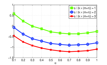
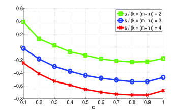
We first note that three sampling methods $\ell_{1}$, $\ell_{2}$, and hybrid-$(\ell_{1},\ell_{2})$, perform identically on noiseless data ${\bm{\mathrm{D}}}$. We report the total probability of sampling noisy elements in ${\bm{\mathrm{A}}}={\bm{\mathrm{D}}}+\textbf{N}$ (elements which are zeros in ${\bm{\mathrm{D}}}$). $\ell_{1}$ sampling shows the highest susceptibility to noise, whereas, small-valued noisy elements are suppressed in $\ell_{2}$. Hybrid-$(\ell_{1},\ell_{2})$ sampling, with $\alpha<1$, samples mostly from true data elements, and thus captures the low-rank structure of the data better than $\ell_{1}$. The optimal mixing parameter $\alpha^{*}$ maintains the right balance between $\ell_{2}$ sampling and $\ell_{1}$ regularization and gives the smallest sample size to achieve a desired accuracy. Table 3 summarizes $\alpha^{*}$ for various data sets. Achlioptas et al. (2013) argued that, as long as $\text{rs}_{0}({\bm{\mathrm{X}}})\geq\text{rs}_{1}({\bm{\mathrm{X}}})$, $\ell_{1}$ sampling is better than $\ell_{2}$ (even with truncation). Our results on $\alpha^{*}$ in Table 3 confirm this condition. Moreover, our method can derive the right blend of $\ell_{1}$ and $\ell_{2}$ sampling even when the above condition fails. In this sense, we generalize the results of Achlioptas et al. (2013).

	$\epsilon=0.05$	$\epsilon=0.75$	$\text{rs}_{0}\geq\text{rs}_{1}$
${\bm{\mathrm{A}}}_{0.05}$	0.62	0.69	no
${\bm{\mathrm{A}}}_{0.1}$	0.63	0.70	no
TechTC1	1	1	yes
TechTC2	1	1	yes
TechTC3	1	1	yes
TechTC4	1	1	yes
Digit	0.20	0.74	no
Stock	0.74	0.75	no

Table 3: $\alpha^{*}$ for various data sets ($\epsilon$ is the desired relative-error accuracy). The last column compares $\alpha^{*}$ with the condition established by Achlioptas et al. (2013). Whenever $\text{rs}_{0}\geq\text{rs}_{1}$, Achlioptas et al. (2013) show that $\ell_{1}$ sampling is always better than $\ell_{2}$ sampling, and we find $\alpha^{*}=1$ ($\ell_{1}$ sampling). However, when $\text{rs}_{0}<\text{rs}_{1}$, $\alpha^{*}<1$ and our hybrid sampling is strictly better.

Figure 4 plots $\mathcal{E}={\mbox{}\|{\bm{\mathrm{A}}}-\tilde{{\bm{\mathrm{A}}}}\|_{2}}/{\mbox{}\|{\bm{\mathrm{A}}}\|_{2}}$ for various values of $\alpha$ and sample size $s$ for various datasets. It clearly shows our optimal hybrid sampling is superior to $\ell_{1}$ or $\ell_{2}$ sampling.

(a) ${\bm{\mathrm{A}}}_{0.05}$

(b) ${\bm{\mathrm{A}}}_{0.1}$

(c) Digit

(d) Stock

Figure 4: Approximation quality of sparse sketch $\tilde{{\bm{\mathrm{A}}}}$: hybrid-$(\ell_{1},\ell_{2})$ sampling, for various $\alpha$ and different sample size $s$, are shown. $x$-axis is $\alpha$, and $y$-axis plots ${\mbox{}\|{\bm{\mathrm{A}}}-\tilde{{\bm{\mathrm{A}}}}\|_{2}}/{\mbox{}\|{\bm{\mathrm{A}}}\|_{2}}$ (in log₂ scale such that larger negative values indicate better quality). Each figure corresponds to a dataset: (a) ${\bm{\mathrm{A}}}_{0.05}$, (b) ${\bm{\mathrm{A}}}_{0.1}$, (c) Digit, and (d) Stock. We set $k=5$ for synthetic data, $k=3$ for Digit data, and $k=1$ for Stock data. Choice of $k$ is close to the stable rank of the data.

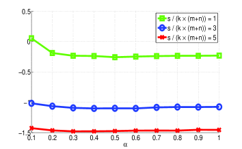
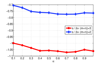
We also compare the quality of sparse sketches produced via our hybrid sampling with that of $\ell_{2}$ sampling with truncation. We use two predetermined truncation parameters, $\epsilon=0.1$ and $\epsilon=0.01$, for $\ell_{2}$ sampling. First, $\ell_{2}$ sampling without truncation turns out to be the worst for all datasets. $\ell_{2}$ with $\epsilon=0.01$ appears to produce sparse sketch $\tilde{{\bm{\mathrm{A}}}}$ that is as bad as $\ell_{2}$ without truncation for ${\bm{\mathrm{A}}}_{0.1}$ and ${\bm{\mathrm{A}}}_{0.05}$. However, $\ell_{2}$ with $\epsilon=0.1$ shows better performance than hybrid sampling, for ${\bm{\mathrm{A}}}_{0.1}$ and ${\bm{\mathrm{A}}}_{0.05}$, because this choice of $\epsilon$ turns out to be an appropriate threshold to zero-out most of the noisy elements. We must point out that, in this example, we control the noise, and we know what a good threshold may look like. However, in reality we have no control over the noise. Therefore, choosing the right threshold for $\ell_{2}$, without any prior knowledge, is an improbable task. For real datasets, it turns out that hybrid-$(\ell_{1},\ell_{2})$-hybrid sampling using $\alpha^{*}$ outperforms $\ell_{2}$ sampling with the predefined thresholds for various sample sizes.

We compare the quality of Algorithm 3 producing an iterative estimate of $\alpha^{*}$ in a very restricted set up, i.e., one pass over the elements of data using $O(s)$ memory. Table 4 lists $\tilde{\alpha}$, the estimated $\alpha^{*}$, for some of the datasets, for two choices of $s$ using 10 iterations. We compare these values with the plots in Figure 4 where the results are generated without any restriction of size of memory or number of pass over the elements of the datasets.

	${s\over k\cdot(m+n)}=2$	${s\over k\cdot(m+n)}=3$
${\bm{\mathrm{A}}}_{0.05},k=5$	0.54	0.48
${\bm{\mathrm{A}}}_{0.1},k=5$	0.55	0.5
Digit, $k=3$	0.69	0.89
Stock, $k=1$	1	1

Table 4: Values of $\tilde{\alpha}$ (estimated $\alpha^{*}$ using Algorithm 3) for various data sets using one pass over the elements of data and $O(s)$ memory. We use $\epsilon=0.05$, $\delta=0.1$.

Finally, we compare our hybrid-$(\ell_{1},\ell_{2})$ sampling with element-wise leverage score sampling (similar to Chen et al. (2014)) to produce quality sparse sketches from low-rank matrices. For this, we construct a $500\times 500$ low-rank power-law matrix, similar to Chen et al. (2014), as follows: ${\bm{\mathrm{A}}}_{pow}={\bm{\mathrm{D}}}{\bm{\mathrm{X}}}{\bm{\mathrm{Y}}}^{T}{\bm{\mathrm{D}}}$, where, matrices ${\bm{\mathrm{X}}}$ and ${\bm{\mathrm{Y}}}$ are $500\times 5$ i.i.d. Gaussian $\mathcal{N}(0,1)$ and ${\bm{\mathrm{D}}}$ is a diagonal matrix with power-law decay, ${\bm{\mathrm{D}}}_{ii}=i^{-\gamma}$, $1\leq i\leq 500$. The parameter $\gamma$ controls the ‘incoherence’ of the matrix, i.e., larger values of $\gamma$ makes the data more ‘spiky’. Table 5 lists the quality of sparse sketches produced via the two sampling methods.

	${s\over k(m+n)}$	hybrid-$(\ell_{1},\ell_{2})$	$p_{lev}$
$\gamma=0.5$	3	42%	58%
	5	31%	43%
$\gamma=0.8$	3	15%	43%
	5	12%	40%
$\gamma=1.0$	3	8%	42%
	5	6%	39%

Table 5: Sparsification quality $\mbox{}\|{\bm{\mathrm{A}}}_{pow}-\tilde{{\bm{\mathrm{A}}}}_{pow}\|_{2}/\mbox{}\|{\bm{\mathrm{A}}}_{pow}\|_{2}$ for low-rank ‘power-law’ matrix ${\bm{\mathrm{A}}}_{pow}$ ($k=5$). We compare the quality of hybrid-$(\ell_{1},\ell_{2})$ sampling and leverage score sampling for two sample sizes. We note (average) $\alpha^{*}$ of hybrid-$(\ell_{1},\ell_{2})$ distribution for data ${\bm{\mathrm{A}}}_{pow}$ using $\epsilon=0.05,\delta=0.1$. For $\gamma=0.5,0.8,1.0$, we have $\alpha^{*}=0.11,0.72,0.8$, respectively.

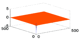
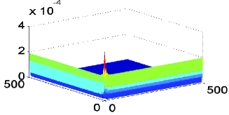
We note that, with increasing $\gamma$ leverage scores get more aligned with the structure of the data, resulting in gradually improving approximation quality, for the same sample size. Larger $\gamma$ produces more variance in data elements. $\ell_{2}$ component of our hybrid distribution bias us towards the larger data elements, while $\ell_{1}$ works as a regularizer to maintain the variance of the sampled (and rescaled) elements. With increasing $\gamma$ we need more regularization to counter the problem of rescaling. Interestingly, our optimal parameter $\alpha^{*}$ adapts itself with this changing structure of data, e.g. for $\gamma=0.5,0.8,1.0$, we have $\alpha^{*}=0.11,0.72,0.8$, respectively. This shows the benefit of our parameterized hybrid distribution to achieve a superior approximation quality. Figure 5 shows the structure of the data ${\bm{\mathrm{A}}}_{pow}$ for $\gamma=1.0$ along with the optimal hybrid-$(\ell_{1},\ell_{2})$ distribution and leverage score distribution $p_{lev}$. The figure suggests our optimal hybrid distribution is better aligned with the structure of the data, requiring smaller sample size to achieve a desired sparsification accuracy.

We also compare the performance of the two sampling methods, optimal hybrid and leverage scores, on rank-truncated Digit data. It turns out that projection of Digit data onto top three principal components preserve the separation of digit categories. Therefore, we rank-truncate Digit data via SVD using rank three. Table 6 shows the superior quality of sparse sketches produced via optimal hybrid-$(\ell_{1},\ell_{2})$ sampling for this rank-truncated digit data.

	Hybrid-$(\ell_{1},\ell_{2})$	$p_{lev}$
${s\over k(m+n)}=3$	44%	61%
${s\over k(m+n)}=5$	34%	47%

Table 6: Sparsification quality $\mbox{}\|{\bm{\mathrm{A}}}-\tilde{{\bm{\mathrm{A}}}}\|_{2}/\mbox{}\|{\bm{\mathrm{A}}}\|_{2}$ for rank-truncated Digit matrix ($k=3$). We compare the optimal hybrid-$(\ell_{1},\ell_{2})$ sampling and leverage score sampling for two sample sizes.

Finally, Table 7 shows the superiority of optimal hybrid-$(\ell_{1},\ell_{2})$ sampling for rank-truncated (rank 5) ${\bm{\mathrm{A}}}_{0.1}$ matrix for matrix sparsification.

	Hybrid-$(\ell_{1},\ell_{2})$	$p_{lev}$
${s\over k(m+n)}=3$	25%	80%
${s\over k(m+n)}=5$	21%	62%

Table 7: Sparsification quality $\mbox{}\|{\bm{\mathrm{A}}}-\tilde{{\bm{\mathrm{A}}}}\|_{2}/\mbox{}\|{\bm{\mathrm{A}}}\|_{2}$ for rank-truncated ${\bm{\mathrm{A}}}_{0.1}$ matrix ($k=5$). We compare the optimal hybrid-$(\ell_{1},\ell_{2})$ sampling and leverage score sampling using two sample sizes.

(a) Low-rank data ${\bm{\mathrm{A}}}_{pow}$

(b) Element-wise leverage scores for ${\bm{\mathrm{A}}}_{pow}$

(c) Optimal hybrid distribution for ${\bm{\mathrm{A}}}_{pow}$

Figure 5: Comparing optimal hybrid-$(\ell_{1},\ell_{2})$ distribution with leverage scores $p_{lev}$ for data ${\bm{\mathrm{A}}}_{pow}$ for $\gamma=1.0$. (a) Structure of ${\bm{\mathrm{A}}}_{pow}$, (b) distribution $p_{lev}$, (c) optimal hybrid-$(\ell_{1},\ell_{2})$ distribution. Our optimal hybrid distribution is more aligned with the structure of the data, requiring much smaller sample size to achieve a given accuracy of sparsification. This is supported by Table 5.

5.4.2 Quality of Fast PCA

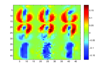
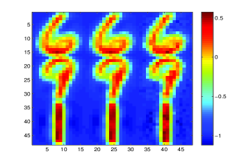
We investigate the quality of fast PCA approximation (Algorithm 4) for Digit data and ${\bm{\mathrm{A}}}_{0.1}$. We set $r=30\cdot k$ for the random projection matrix ${\bm{\mathrm{A}}}_{G}$ to achieve a comparable runtime of $\mathcal{G}$ with $\mathcal{H}$. Figure 6(a) shows the PCA (exact and approximate) for Digit data. Also, we consider visualization of the projected data onto top three principal components (exact and approximate) in Figure 6(b). In Figure 6(b), we form an average digit for each digit category by taking the average of pixel intensities in the projected data over all the digit samples in each category. Similarly, Figure 7 shows the visual results for data ${\bm{\mathrm{A}}}_{0.1}$ (we set $k=5$). Finally, Table 8 lists the gain in computation time for Algorithm 4 due to sparsification.

(a) PCA’s

(b) Projected data onto the PCA’s

Figure 6: Approximation quality of fast PCA (Algorithm 4) on Digit data. (a) Visualization of principal components as $16\times 16$ image. Principal components are ordered from the top row to the bottom. First column of PCA’s are exact $\mathcal{A}$. Second column of PCA’s are $\mathcal{H}$ computed on sparsified data using $\sim$ 7% of all the elements via optimal hybrid sampling. Third column of PCA’s are $\mathcal{G}$ computed on ${\bm{\mathrm{A}}}_{G}$. Visually, $\mathcal{H}$ is closer to $\mathcal{A}$. (b) Visualization of projected data onto top three PCA’s. First column shows the average digits of projected actual data onto the exact PCA’s $\mathcal{A}$. Second column is the average digits of projected actual data onto approximate PCA’s (of sampled data) $\mathcal{H}$. We observe a similar quality of average digits of projected actual data onto approximate PCA’s $\mathcal{G}$ of ${\bm{\mathrm{A}}}_{G}$. Third column shows the average digits for projected sparsified data onto approximate PCA’s $\mathcal{H}$.

Figure 7: Approximation quality of fast PCA (Algorithm 4) for data ${\bm{\mathrm{A}}}_{0.1}$. Visualization of projected data onto top five PCA’s. Left image shows the projected actual data onto the exact PCAs $\mathcal{A}$. Middle image is the projection of actual data onto approximate PCA’s (of sampled data) $\mathcal{H}$. We observe a similar quality of PCA’s $\mathcal{G}$ for ${\bm{\mathrm{A}}}_{G}$. Right image shows the projected sparsified data onto approximate PCA’s $\mathcal{H}$. We use only 6% of all the elements to produce the sparse sketches via optimal hybrid sampling.

	Sparsified Digit	Sparsified ${\bm{\mathrm{A}}}_{0.1}$
Sparsity	93%	94%
$T_{h}/T_{a}/T_{G}$	30/151/36	18/73/36

Table 8: Computational gain of Algorithm 4 comparing to exact PCA. We report the computation time of MATLAB function ‘svds(${\bm{\mathrm{A}}}$,$k$)’ for actual data ($T_{a}$), sparsified data ($T_{h}$), and random projection data ${\bm{\mathrm{A}}}_{G}$ ($T_{G}$). We use only 7% and 6% of all the elements of Digit data and ${\bm{\mathrm{A}}}_{0.1}$, respectively, to construct respective sparse sketches.

5.5 Conclusion

Overall, the experimental results demonstrate the quality of the algorithms presented here, indicating the superiority of our approach to other extreme choices of element-wise sampling methods, such as, $\ell_{1}$ and $\ell_{2}$ sampling. Also, we demonstrate the theoretical and practical usefulness of hybrid-$(\ell_{1},\ell_{2})$ sampling for fundamental data analysis tasks such as fast computation of PCA. Finally, our method outperforms element-wise leverage scores for the sparsification of various low-rank synthetic and real data matrices.

References

- Achlioptas and McSherry (2001) D. Achlioptas and F. McSherry. Fast computation of low rank matrix approximations. In Proceedings of Symposium on the Theory of Computing, pages 611–618, 2001.
- Achlioptas and McSherry (2007) D. Achlioptas and F. McSherry. Fast computation of low-rank matrix approximations. Journal of the ACM, page 54(2):9, 2007.
- Achlioptas et al. (2013) D. Achlioptas, Z. Karnin, and E. Liberty. Matrix entry-wise sampling: Simple is best. In http://citeseerx.ist.psu.edu/viewdoc/download?doi=10.1.1.297.576&rep=rep1&type=pdf, 2013.
- Arora et al. (2006) S. Arora, E. Hazan, and S. Kale. A Fast Random Sampling Algorithm for Sparsifying Matrices. In Approximation, Randomization, and Combinatorial Optimization. Algorithms and Techniques, pages 272 –279, vol 4110. Springer, 2006.
- Chen et al. (2014) Y Chen, S Bhojanapalli, S Sanghavi, and R Ward. Coherent Matrix Completion. Proceedings of International Conference on Machine Learning, pages 674–682, 2014.
- Drineas and Zouzias (2011) P. Drineas and A. Zouzias. A note on element-wise matrix sparsification via a matrix-valued Bernstein inequality. In Information Processing Letters, pages 385 –389, 111(8), 2011.
- Drineas et al. (2006) P. Drineas, R. Kannan, and M. W. Mahoney. Fast monte carlo algorithms for matrices I: approximating matrix multiplication. In SIAM Journal on Computing, pages 132–157, 36(1), 2006.
- Gabrilovich and Markovitch (2004) E. Gabrilovich and S. Markovitch. Text categorization with many redundant features: using aggressive feature selection to make SVMs competitive with C4.5. In Proceedings of International Conference on Machine Learning, 2004.
- Hull (1994) J. J. Hull. A database for handwritten text recognition research. In IEEE Transactions on Pattern Analysis and Machine Intelligence, pages 550–554, 16(5), 1994.
- Kundu and Drineas (2014) A. Kundu and P. Drineas. A Note on Randomized Element-wise Matrix Sparsification. In http://arxiv.org/pdf/1404.0320v1.pdf, 2014.
- Recht (2011) B. Recht. A simpler approach to matrix completion. In The Journal of Machine Learning Research, pages 3413–3430, 12, 2011.