Recursion in multiplet bases for tree-level MHV gluon amplitudes

Abstract

We investigate the construction of tree-level MHV gluon amplitudes in multiplet bases using BCFW recursion. The multiplet basis decomposition can either be obtained by decomposing results derived in (for example) the DDM basis or by formulating the recursion directly in the multiplet basis. We focus on the latter approach and show how to efficiently deal with the color structure appearing in the recursion. For illustration, we also explicitly calculate the four-, five- and six-gluon amplitudes.

1 Introduction

Scattering amplitudes are essential tools for understanding multi-parton processes in high energy physics. Traditional calculations based on Feynman diagrams have proven extremely cumbersome due to the large number of diagrams and the correlation of the color and kinematic factors. To simplify the calculations of amplitudes, large efforts have been made, including the development of the spinor helicity formalism Berends:1981rb ; Causmaecker:1981bg ; Kleiss:1985yh ; Xu:1986xb ; Gunion:1985vca , the Berends-Giele recursion for off-shell currents Berends:1987me , various forms of color decompositions Cvi76 ; Cvitanovic:1980bu ; Dittner:1972hm ; Zeppenfeld:1988bz ; Paton:1969je ; Berends:1987cv ; Mangano:1987xk ; Mangano:1988kk ; Kosower:1988kh ; Nagy:2007ty ; Sjodahl:2009wx ; Alwall:2011uj ; Sjodahl:2014opa ; Platzer:2012np ; DelDuca:1999ha ; DelDuca:1999rs ; Kanaki:2000ms ; Maltoni:2002mq ; Keppeler:2012ih ; Sjodahl:2015qoa ; Kol:2014yua , the Parke-Taylor formula for color-ordered maximally helicity violating (MHV) amplitudes Parke:1986gb ; Berends:1987me , the Kleiss-Kuijf (KK) relation Kleiss:1988ne , the twistor string method Witten:2003nn , Cachazo-Svrcek-Witten (CSW) rules Cachazo:2004kj , Britto-Cachazo-Feng-Witten (BCFW) recursion Britto:2004ap ; Britto:2005fq and the Bern-Carrasco-Johansson (BCJ) relation Bern:2008qj between color-ordered amplitudes. Reviews of related topics can be found in Mangano:1990by ; Dixon:1996wi ; Cachazo:2005ga ; Bern:2007dw ; Feng:2011np ; Peskin:2011in ; Benincasa:2013faa ; Ellis:2011cr ; Elvang:2013cua .

In most of this work the color decomposition plays an important role for understanding and simplifying scattering amplitudes. Several types of color decompositions for gluon amplitudes are available, most notably the trace basis decomposition Paton:1969je ; Berends:1987cv ; Mangano:1987xk ; Mangano:1988kk ; Kosower:1988kh ; Nagy:2007ty ; Sjodahl:2009wx ; Alwall:2011uj ; Sjodahl:2014opa ; Platzer:2012np , the Del Duca-Dixon-Maltoni (DDM) basis decomposition DelDuca:1999ha ; DelDuca:1999rs and the color-flow basis decomposition Maltoni:2002mq ; Kanaki:2000ms . Since recently it is also known how to construct orthogonal group theory based multiplet bases for any number of quarks and gluons Keppeler:2012ih .

While the topic of scattering amplitude recursion relations has been explored for the kinematic factors (the color-ordered amplitudes) of the first three bases for a while Berends:1987me ; Britto:2004ap ; Britto:2005fq , this field is unknown territory in the context of multiplet bases. In the present paper we take the first step to remedy this by showing how to use BCFW recursion relations for multiplet bases in the case of MHV amplitudes in pure Yang-Mills theory. To set the stage for this task, we first give a brief overview of the standard color decompositions and the present status of recursion strategies.

• Trace bases
  The color decomposition for a tree-level gluon amplitude with $n$ gluons in trace bases is given by Paton:1969je ; Berends:1987cv ; Mangano:1987xk ; Mangano:1988kk ; Kosower:1988kh ; Nagy:2007ty ; Sjodahl:2009wx ; Alwall:2011uj ; Sjodahl:2014opa ,

  $$\mathcal{M}(g_{1},g_{2},\dots,g_{n})=g^{n-2}\left(1\over\sqrt{T_{R}}\right)^{n}\sum\limits_{\sigma,\mbox{ \scriptsize s.t. }\sigma_{1}=1}\mathop{\rm Tr}(t^{g_{1}}t^{g_{\sigma_{2}}}\dots t^{g_{\sigma_{n}}})A(\sigma),~{}~{}$$ (1)

  where we have used a general generator normalization $\operatorname*{\mathrm{tr}}(t^{a}t^{b})=T_{R}\delta^{a\,b}$. The cyclicity of the trace allows for fixing $\sigma_{1}=1$, thus leaving $(n-1)!$ color structures in the sum. The kinematic factors, $A(\sigma)$ are called color-ordered amplitudes and can be calculated from the color-ordered Feynman rules, also known as the color-stripped Feynman rules. These bases (spanning sets) are easily extended to loop level, upon which products of traces occur, Bern:1990ux ; Nagy:2007ty ; Sjodahl:2009wx ; Sjodahl:2014opa , as well as to processes with quarks, requiring open quark-lines in addition to the traces Kosower:1988kh ; Mangano:1988kk ; Mangano:1990by ; Nagy:2007ty ; Sjodahl:2009wx ; Sjodahl:2014opa .

• Color-flow bases
  An approach similar to the trace basis approach is given by the color-flow bases Maltoni:2002mq ; Kanaki:2000ms . Here the gluon field is rewritten in terms of the fundamental representation $(A_{\mu})^{i}_{j}$, $i,j=1,..,N_{c}$, for $N_{c}$ colors, and the color structure is described in terms of flow of color. For tree-level gluon amplitudes the color decomposition is given by

  $$\mathcal{M}(g_{1},g_{2},\dots,g_{n})={g^{n-2}\left(1\over\sqrt{T_{R}}\right)^{n}}\sum\limits_{\sigma,\mbox{ \scriptsize s.t. }\sigma_{1}=1}\delta^{i_{\sigma_{1}}}_{j_{\sigma_{2}}}\delta^{i_{\sigma_{2}}}_{j_{\sigma_{3}}}\dots\delta^{i_{\sigma_{n}}}_{j_{\sigma_{1}}}A(\sigma),~{}~{}$$ (2)

  where the sum runs over the $(n-1)!$ permutations from connecting color lines. It is not hard to argue that the amplitudes $A(\sigma)$ are the same as in the trace bases. Similar to the trace bases, these bases are extendable to processes at higher order. Their advantage lies in better scaling properties for Monte Carlo treatment of the color structure Maltoni:2002mq .

• Del Duca-Dixon-Maltoni bases
  Tree-level gluon amplitudes may alternatively be decomposed using the Del Duca-Dixon-Maltoni (DDM) bases DelDuca:1999ha ; DelDuca:1999rs

  $$\mathcal{M}({g_{1}},{g_{2}},\dots,{g_{n}})=g^{n-2}\left(1\over\sqrt{T_{R}}\right)^{n-2}\sum\limits_{\sigma,\mbox{ \scriptsize s.t. }\sigma_{1}=1,\,\sigma_{n}=n}if^{g_{\sigma_{1}}g_{\sigma_{2}}i_{1}}if^{i_{1}g_{\sigma_{3}}i_{2}}\dots if^{i_{n-3}g_{\sigma_{n-1}}g_{\sigma_{n}}}A(\sigma),~{}~{}$$ (3)

  where $\sigma_{1}=1$ and $\sigma_{n}=n$ are fixed. The color-ordered amplitudes $A(\sigma_{1}=1,\sigma_{2},\dots,\sigma_{n-1},\sigma_{n}=n)$ form the so called Kleiss-Kuijf (KK) basis Kleiss:1988ne . All other color-ordered amplitudes, i.e., all the amplitudes in eq. (1) with $\sigma(n)\neq n$, can be expressed in the KK basis using the Kleiss-Kuijf (KK) relation

  $$A(1,\{\alpha\},n,\{\beta\})=(-1)^{n_{\beta}}\sum\limits_{\sigma\in OP(\alpha\bigcup\beta^{T})}A(1,\sigma,n),$$ (4)

  where $n_{\beta}$ denotes the number of indices in the set $\beta$, and the sum runs over all possible permutations which keep the relative order of indices in the index set $\alpha$ and reverse the relative index order in the index set $\beta$, while allowing for all possible relative orderings between each $\alpha_{i}$ with respect to each $\beta_{j}$.

  Compared to the trace bases and color-flow bases there is clearly an advantage in needing only $(n-2)!$ rather than $(n-1)!$ spanning vectors. The color decomposition in DDM bases can also be extended to one-loop level and to amplitudes containing a quark-antiquark pair DelDuca:1999rs . A proof of the KK relation can be found in DelDuca:1999rs , the BCFW approach to the KK relation is presented in Feng:2010my , and the Berends-Giele recursion approach for the off-shell KK relation was given in Fu:2012uy .

In the three color decompositions above, the kinematic factors can be expressed using the color-ordered amplitudes that were defined in the trace bases decomposition, eq. (1). Employing BCFW recursion, one can express these amplitudes in terms of products of lower point on-shell color-ordered amplitudes. Specifically, for the $n$-gluon color-ordered tree amplitude $A(1,2,3,\dots,n)$, if we shift the momenta of gluon $1$ and $n$ using some complex four-vector $q$ and some complex variable $z$,

$$\widehat{p}_{1}(z)=p_{1}-zq,~{}~{}\widehat{p}_{n}(z)=p_{n}+zq,~{}~{}$$ (5)

such that the gluons $\hat{1}$ and $\hat{n}$ remain on-shell, the color-ordered amplitude $A(1,2,3,\dots,n)$ is given by the BCFW recursion (see figure 1)

$$\raisebox{-0.315pt}{ \includegraphics[scale={0.6}]{figures/BCFW_recursion/BCFW_recursion} }=\sum_{i=2}^{n-2}{\sum_{h=\pm}{\raisebox{-0.27pt}{ \includegraphics[scale={0.6}]{figures/BCFW_recursion/BCFW_recursion_split} }}}$$

Figure 1: BCFW recursion for color-ordered tree-level gluon amplitudes.

$$A\left(1,2,\dots,n\right)$$ (6)

$$= \sum\limits_{i=2}^{n-2}\sum\limits_{h=\pm}A\left(\widehat{1}(z_{i}),2,\dots,i,-\widehat{P}^{h}_{\widehat{1}(z_{i}),2,\dots,i}(z_{i})\right){i\over P^{2}_{1,2,\dots,i}}A\left(\widehat{P}^{-h}_{\widehat{1}(z_{i}),2,\dots,i},i+1,\dots,n-1,\widehat{n}(z_{i})\right),$$

where, $P_{1,2,\dots,i}=\sum\limits_{k=1}^{i}p_{k}$. For a given $i$, $z_{i}$ can be solved from

$$\widehat{P}^{2}_{\widehat{1},2,\dots,i}(z_{i})=\left(p_{1}+p_{2}+\dots+p_{i}-z_{i}q\right)^{2}=0.$$ (7)

While the trace bases, the color-flow bases and the DDM bases are conceptually simple and well-established in the literature, they all suffer from being non-orthogonal (unless $N_{c}\rightarrow\infty$), and – in an $N_{c}=3$ sense – non-minimal. The bases being non-orthogonal implies that the squaring of tree-level color structures involves $(n-1)!^{2}$ terms in the case of the trace and color-flow bases, and $(n-2)!^{2}$ terms for the pure Yang-Mills specific DDM bases. Going to arbitrary order in perturbation theory, new color structures appear and the number of vectors (neglecting charge conjugation invariance) increases up to $\mbox{subfactorial}(n)\approx(n!/e)$ in the trace bases Keppeler:2012ih . For practical purposes this means that it is hard to treat the color structure of processes involving more than $\sim 8$ gluons plus $q\overline{q}$-pairs exactly, and currently the most efficient technique for multi-parton calculations is probably to sample color structures in the color-flow basis by Monte Carlo techniques Maltoni:2002mq .

One way to cure the bad scaling involved in the squaring step is to use orthogonal bases. In the case of few partons, such bases, based on the decomposition of the color structure into irreducible representations, have been around for a while Sotiropoulos:1993rd ; Kidonakis:1998nf ; Kyrieleis:2005dt ; Dokshitzer:2005ig ; Sjodahl:2008fz ; Beneke:2009rj , but a general strategy for basis construction based on multiplets was presented only recently Keppeler:2012ih . Below we give an overview of their key properties.

• Multiplet bases
  These bases are based on subgrouping sets of partons and forcing the parton sets to transform under irreducible representations of SU($N_{c}$). By applying the same subgrouping procedure to all basis vectors, orthogonal basis vectors are obtained.

  The decomposition into these bases (to any order in perturbation theory) may be written

  $$\mathcal{M}(g_{1},g_{2},\dots,g_{n})\sim\sum\limits_{\alpha}\mathbf{V}^{\alpha}A^{\alpha},~{}~{}$$ (8)

  where $\alpha$ is some (collective) index of the basis vectors describing the involved representations and $A^{\alpha}$ are the kinematic factors, clearly not equal to the $A(\sigma)$ in eqs. (1-3).

  As the multiplet bases have no direct connection to tree-level color structure, they do not typically span a minimal set for tree-level color structure alone. Instead they are applicable to any order, and are (or can trivially be made) minimal for any finite $N_{c}$, leading to a significant reduction in dimension for a large number of partons (see table 1).

As the multiplet basis vectors $\mathbf{V}^{\alpha}$ do not (generally) have any cyclic symmetry under exchange of gluon indices, one can not expect recursion relations as simple as for the trace basis to hold. On the other hand, being orthogonal, multiplet bases speed up the squaring of amplitudes very significantly. We thus expect to gain in the squaring step, at the expense of a more intricate color decomposition. This decomposition – in a recursion context – is the topic of the present paper, and we will discuss two different ways of achieving it.

• Clearly one strategy is to express the basis vectors in any of the bases where the recursion is known in terms of the relevant multiplet basis. While this strategy – which in principle is nothing but a change of basis – is straight forward, the gain in computation time is unclear as it involves decomposing $(n-1)!$ or $(n-2)!$ color structures into an exponentially growing number of basis vectors. In theory, the exponential times the factorial does scale better than the factorial square involved in squaring amplitudes in the non-orthogonal standard bases. In reality, however, this difference only becomes significant for a relatively large number of gluons, (cf. table 1). Directly rewriting recursion results obtained in other bases may, however, still be beneficial if one color factor (for example one trace or one DDM color factor) can be rewritten as a linear combination of a small number of multiplet basis vectors, and the non-vanishing projections can be identified quickly. For tree-level gluon amplitudes, the best option is likely to use the smaller DDM basis eq. (3).

  In principle, for tree-level processes with only gluons it is also possible to use the Bern-Carrasco-Johansson relation Bern:2008qj (the BCJ relation has been proved in both string theory BjerrumBohr:2009rd ; Stieberger:2009hq and field theory Feng:2010my ; Tye:2010kg ; Chen:2011jxa ) to reduce the color-ordered amplitudes in a smaller basis of $(n-3)!$ color-ordered amplitudes. However, this relation will introduce complicated kinematic factors which are functions of the external momenta Bern:2008qj . Although, there has been extensions of the BCJ relation to cases with fermions e.g., Sondergaard:2009za ; Melia:2013epa , there is no general expression for the BCJ relation in the presence of (fundamental representation) quarks. Since the long term goal of this work is to pursue recursion for processes involving quarks as well, we will therefore not further consider BCJ relations.

• The second approach is to perform the recursion directly in the multiplet basis. Once we know the multiplet basis decompositions for amplitudes for fewer gluons and relations for decomposing the color structure appearing in the BCFW-recursion, we can derive a recursion relation for the kinematic factors $A^{\alpha}$ via the BCFW recursion for the color-dressed amplitudes.

In the following, we will demonstrate the decomposition using the above strategies. In section 2, we calculate the kinematic factors $A^{\alpha}$ by evaluating scalar products. Section 3 provides a derivation of color-dressed BCFW recursion, followed by a recursion relation for the color structure of MHV gluon amplitudes formulated in the multiplet basis. This finally allows us to derive the BCFW recursion for the kinematic factors $A^{\alpha}$ for any number of gluons. In section 4, we conclude and discuss natural extensions.

2 Evaluation by scalar products

In this section, we derive the multiplet basis expansion by comparing the color factors in multiplet bases to those in DDM or trace bases. The general framework for this construction is as follows:

• The color vectors (including powers of $T_{R}$) in the DDM or trace basis (or, in general, any spanning set in which the recursion is known) can be expanded in the multiplet basis vectors,

  $$\mathbf{c}^{\sigma}=\sum\limits_{\alpha}a^{\alpha\sigma}\mathbf{V}^{\alpha},~{}~{}$$ (9)

  where the coefficients are given by scalar products of these two kinds of color factors

  $$a^{\alpha\sigma}=\langle\mathbf{V}^{\alpha}|\mathbf{c}^{\sigma}\rangle.~{}~{}$$ (10)

  The scalar product is given by summing over all external color indices, i.e., for arbitrary color structures $\mathbf{c}^{1}$ and $\mathbf{c}^{2}$,

  $$\langle\mathbf{c}^{1}|\mathbf{c}^{2}\rangle=\sum_{a_{1},\,a_{2},\,...}(\mathbf{c}^{1}{}_{a_{1}\,a_{2}...})^{*}\,\mathbf{c}^{2}{}_{a_{1}\,a_{2}...},$$ (11)

  with $a_{i}=1,\ldots,N_{c}$ if parton $i$ is a quark or antiquark and $a_{i}=1,\ldots,N_{c}^{2}-1$ if parton $i$ is a gluon.

• Substituting the expression eq. (9) into the DDM decomposition, eq. (3), or the trace basis decomposition, eq. (1), and collecting the kinematic factors corresponding to a given basis vector $\mathbf{V}^{\alpha}$ in the multiplet basis, the color-dressed amplitude can be stated as

  $${\cal M}(g_{1},g_{2},\dots,g_{n})=g^{n-2}\sum\limits_{\alpha}\left[\sum\limits_{\sigma}a^{\alpha\sigma}A(\sigma)\right]\mathbf{V}^{\alpha}.~{}~{}$$ (12)

  Comparing the above expression to the multiplet basis expansion eq. (8), we can read off the kinematic factor multiplying the basis vector $\mathbf{V}^{\alpha}$

  $$A^{\alpha}=\sum\limits_{\sigma}a^{\alpha\sigma}A(\sigma).~{}~{}$$ (13)

In principle, one can use this method to derive the multiplet basis expansions for an arbitrary number of external legs with arbitrary helicity configuration. We have calculated the multiplet basis decompositions for up to six gluons, and demonstrate the calculations in the three- and four-gluon cases below. The five- and six-gluon cases are treated using multiplet basis recursion in section 3.

2.1 The three-gluon amplitude

For three gluons the multiplet basis can be chosen as

$$\mathbf{V}_{g_{1}\,g_{2}\,g_{3}}^{8s} = d^{g_{1}g_{3}g_{2}}=\frac{1}{T_{R}}[\mathop{\rm Tr}(t^{g_{1}}t^{g_{3}}t^{g_{2}})+\mathop{\rm Tr}(t^{g_{1}}t^{g_{2}}t^{g_{3}})],$$

$$\mathbf{V}_{g_{1}\,g_{2}\,g_{3}}^{8a} = if^{g_{1}g_{3}g_{2}}=\frac{1}{T_{R}}[\mathop{\rm Tr}(t^{g_{1}}t^{g_{3}}t^{g_{2}})-\mathop{\rm Tr}(t^{g_{1}}t^{g_{2}}t^{g_{3}})],$$ (14)

making it orthogonal but not normalized. From these two equations, we get

$$\mathop{\rm Tr}(t^{g_{1}}t^{g_{3}}t^{g_{2}})=\frac{T_{R}}{2}\left[d^{g_{1}g_{3}g_{2}}+if^{g_{1}g_{3}g_{2}}\right],~{}~{}\mathop{\rm Tr}(t^{g_{1}}t^{g_{2}}t^{g_{3}})=\frac{T_{R}}{2}\left[d^{g_{1}g_{3}g_{2}}-if^{g_{1}g_{3}g_{2}}\right].$$ (15)

Thus the three-gluon multiplet basis expansion is given by

$$\mathcal{M}({g_{1}},{g_{2}},{g_{3}}) = g\left(1\over\sqrt{T_{R}}\right)^{3}\ \frac{T_{R}}{2}[d^{g_{1}g_{3}g_{2}}+if^{g_{1}g_{3}g_{2}}]A(1,3,2)+g\left(1\over\sqrt{T_{R}}\right)^{3}\frac{T_{R}}{2}[d^{g_{1}g_{3}g_{2}}-if^{g_{1}g_{3}g_{2}}]A(1,2,3)$$ (16)

$$= g\frac{1}{2\sqrt{T_{R}}}d^{g_{1}g_{3}g_{2}}[A(1,3,2)+A(1,2,3)]+g\frac{1}{2\sqrt{T_{R}}}if^{g_{1}g_{3}g_{2}}[A(1,3,2)-A(1,2,3)].$$

Since $A(1,2,3)$ is antisymmetric under $1\leftrightarrow 2$ we find

$$A^{8s}=0,\quad A^{8a}={1\over\sqrt{T_{R}}}A(1,3,2),$$ (17)

where we note that the first equation can be seen as a manifestation of charge conjugation invariance (cyclic reflection), and that the second color factor is precisely the amplitude for the (only) vector in the DDM basis.

2.2 The four-gluon amplitude

In the four-gluon case, we start from the DDM decomposition with $1$ and $2$ as the fixed legs

$$\mathcal{M}(g_{1},g_{2},g_{3},g_{4})=g^{2}{1\over T_{R}}if^{g_{1}g_{2}i_{1}}if^{i_{1}g_{3}g_{4}}A(1,2,3,4)+g^{2}{1\over T_{R}}if^{g_{1}g_{3}i_{1}}if^{i_{1}g_{2}g_{4}}A(1,3,2,4).$$ (18)

Using ColorMath Sjodahl:2012nk to evaluate the scalar products in eq. (10) this is decomposed into the multiplet basis $\mathcal{V}$

$$\mathcal{V}=\Bigl{\{}\mathbf{V}_{g_{1}\,g_{3};\,g_{2}\,g_{4}}^{1},\mathbf{V}_{g_{1}\,g_{3};\,g_{2}\,g_{4}}^{8s},\mathbf{V}_{g_{1}\,g_{3};\,g_{2}\,g_{4}}^{8a},\mathbf{V}_{g_{1}\,g_{3};\,g_{2}\,g_{4}}^{27},\frac{1}{\sqrt{2}}\left[\mathbf{V}_{g_{1}\,g_{3};\,g_{2}\,g_{4}}^{10}+\mathbf{V}_{g_{1}\,g_{3};\,g_{2}\,g_{4}}^{\overline{10}}\right],\mathbf{V}_{g_{1}\,g_{3};\,g_{2}\,g_{4}}^{0}\Bigr{\}},$$ (19)

given by Keppeler:2012ih ,

$$\mathbf{V}_{g_{1}\,g_{3};\,g_{2}\,g_{4}}^{\alpha}=\frac{1}{\sqrt{d_{\alpha}}}\mathbf{P}^{\alpha}_{g_{1}\,g_{3};\,g_{2}\,g_{4}}$$ (20)

where $\mathbf{P}^{\alpha}$ is the projection operator onto the irreducible representation $\alpha$ with dimension $d_{\alpha}$ Butera:1979na ; Cvi84 ; Cvi08 ; Dokshitzer:2005ig ; Keppeler:2012ih ,

$$\mathbf{P}^{1}_{g_{1}\,g_{3};\,g_{2}\,g_{4}} = \frac{1}{N_{c}^{2}-1}\delta^{{g_{1}\,g_{3}}}\delta^{{g_{2}\,g_{4}}}\,,$$

$$\mathbf{P}^{8s}_{g_{1}\,g_{3};\,g_{2}\,g_{4}} = \frac{N_{c}}{2T_{R}(N_{c}^{2}-4)}d^{{g_{1}g_{3}i_{1}}}d^{{i_{1}g_{2}g_{4}}}\,,$$

$$\mathbf{P}^{8a}_{g_{1}\,g_{3};\,g_{2}\,g_{4}} = \frac{-1}{2N_{c}T_{R}}if^{g_{1}\,g_{3}\,i_{1}}if^{i_{1}\,g_{2}\,g_{4}}\,,$$

$$\mathbf{P}^{27}_{g_{1}\,g_{3};\,g_{2}\,g_{4}} = \frac{1}{4}(\delta^{g_{1}\,i_{1}}\delta^{g_{3}\,i_{2}}+\delta^{g_{1}\,i_{2}}\delta^{g_{3}\,i_{1}})\left[\delta^{i_{1}\,g_{2}}\delta^{i_{2}\,g_{4}}+\frac{1}{T_{R}^{2}}\operatorname*{\mathrm{tr}}(t^{i_{1}}t^{g_{4}}t^{i_{2}}t^{g_{2}})\right]$$

$$-\frac{N_{c}-2}{2N_{c}}\,\mathbf{P}^{8s}_{g_{1}\,g_{3};\,g_{2}\,g_{4}}-\frac{N_{c}-1}{2N_{c}}\,\mathbf{P}^{1}_{g_{1}\,g_{3};\,g_{2}\,g_{4}}\,,$$

$$\mathbf{P}^{10}_{g_{1}\,g_{3};\,g_{2}\,g_{4}} = \frac{1}{4}(\delta^{g_{1}\,i_{1}}\delta^{g_{3}\,i_{2}}-\delta^{g_{1}\,i_{2}}\delta^{g_{3}\,i_{1}})\left[\delta^{i_{1}\,g_{2}}\delta^{i_{2}\,g_{4}}+\frac{1}{T_{R}^{2}}\operatorname*{\mathrm{tr}}(t^{i_{1}}t^{g_{4}}t^{i_{2}}t^{g_{2}})\right]-\frac{1}{2}\,\mathbf{P}^{8a}_{g_{1}\,g_{3};\,g_{2}\,g_{4}}\,,$$

$$\mathbf{P}^{\overline{10}}_{g_{1}\,g_{3};\,g_{2}\,g_{4}} = \frac{1}{4}(\delta^{g_{1}\,i_{1}}\delta^{g_{3}\,i_{2}}-\delta^{g_{1}\,i_{2}}\delta^{g_{3}\,i_{1}})\left[\delta^{i_{1}\,g_{2}}\delta^{i_{2}\,g_{4}}-\frac{1}{T_{R}^{2}}\operatorname*{\mathrm{tr}}(t^{i_{1}}t^{g_{4}}t^{i_{2}}t^{g_{2}})\right]-\frac{1}{2}\,\mathbf{P}^{8a}_{g_{1}\,g_{3};\,g_{2}\,g_{4}}\,,$$

$$\mathbf{P}^{0}_{g_{1}\,g_{3};\,g_{2}\,g_{4}} = \frac{1}{4}(\delta^{g_{1}\,i_{1}}\delta^{g_{3}\,i_{2}}+\delta^{g_{1}\,i_{2}}\delta^{g_{3}\,i_{1}})\left[\delta^{i_{1}\,g_{2}}\delta^{i_{2}\,g_{4}}-\frac{1}{T_{R}^{2}}\operatorname*{\mathrm{tr}}(t^{i_{1}}t^{g_{4}}t^{i_{2}}t^{g_{2}})\right]$$ (21)

$$-\frac{N_{c}+2}{2N_{c}}\,\mathbf{P}^{8s}_{g_{1}\,g_{3};\,g_{2}\,g_{4}}-\frac{N_{c}+1}{2N_{c}}\,\mathbf{P}^{1}_{g_{1}\,g_{3};\,g_{2}\,g_{4}}\,,$$

and the general expressions for the dimensions are

$$d_{8}=N_{c}^{2}-1,\;\;d_{10}=\frac{1}{4}(N_{c}^{4}-5N_{c}^{2}+4),\;\;d_{27}=\frac{1}{4}N_{c}^{2}(N_{c}^{2}+2N_{c}-3)\;\;d_{0}=\frac{1}{4}N_{c}^{2}(N_{c}^{2}-2N_{c}-3).\;\;$$ (22)

Expressed in this basis (which is also electronically attached as an online resource) the amplitude can be stated

$$\mathcal{M}(g_{1},g_{2},g_{3},g_{4})=g^{2}\mathcal{A}\cdot\mathcal{V},$$ (23)

where $\mathcal{A}$ is the kinematic factor,

$$\mathcal{A} = N_{c}\times\Bigl{\{}-2A(1,2,3,4),-\sqrt{\left(N_{c}+1\right)\left(N_{c}-1\right)}A(1,2,3,4),-\sqrt{\left(N_{c}+1\right)\left(N_{c}-1\right)}$$

$$\left[A(1,2,3,4)+2A(1,3,2,4)\right],\sqrt{\left(N_{c}+3\right)\left(N_{c}-1\right)}A(1,2,3,4),0,-\sqrt{\left(N_{c}+1\right)\left(N_{c}-3\right)}A(1,2,3,4)\Bigr{\}}.$$

Note that in the above discussion, we did not specify the helicity of the external legs. When we want to consider the kinematic factor for a particular helicity configuration, e.g., $1^{-},2^{+},3^{+},4^{-}$ we just substitute the corresponding form of the color-ordered amplitudes into eq. (2.2).

A few remarks on the basis are in place. First we note that for $N_{c}=3$ the last basis vector vanishes as it corresponds to a multiplet which only appears for $N_{c}\geq 4$. For four gluons this reduction in dimension due to small $N_{c}$ is rather unimportant, but for large $n$, the difference becomes significant, (cf. table 1).

Then we note that, due to charge conjugation invariance (which at tree-level manifests itself as cyclic reflection in trace bases), the decuplet and anti-decuplet in eq. (19) must multiply the same amplitude, which – at tree-level – vanishes. Charge conjugation invariance is also the reason why the octet vectors corresponding to contracting one antisymmetric structure constant with one symmetric structure constant vanish. This means that the four-gluon basis vectors can be expressed in terms of projectors only. Note, however, this a special feature of the four-gluon basis, it is not generally possible (even for $n$ even), as there are different ways of building up the same multiplet, see for example Keppeler:2012ih .

Finally we point out that although the multiplet decomposed result eq. (2.2) may look somewhat complicated, it is now in an excellent form for squaring. For given helicities and external momenta, the color-ordered amplitudes in eq. (2.2) are just (complex) numbers. To get the full amplitude square, we thus just have to square the coefficients in eq. (2.2) and add them up.

In this particular case of four gluons only, not much is gained by this rewriting, as the scalar product matrix for the DDM basis anyway only involves $2\times 2$ terms. However, for larger bases, where the $2\times 2$ scalar product matrix is replaced by a matrix of dimension $(n-2)!\times(n-2)!$ (or $(n-1)!\times(n-1)!$ for trace bases), avoiding the factorial square is clearly desirable.

Unfortunately, with the naive way of calculating scalar products utilized here, involving direct evaluation of $(n-2)!$ $\times$ (the number of multiplet basis vectors) entries, what is gained in the squaring step for multiplet bases, may be lost in the step of scalar product decomposition. We do note, however, that a more clever procedure for evaluating scalar products, based on the birdtrack method and Wigner $3j$ and $6j$ coefficients Cvi08 ; Sjodahl:2015qoa possibly could change this conclusion. As it is unclear if the scalar product method is beneficial, the remainder of this paper instead focuses on deriving recursion relations directly in the multiplet basis.

3 Recursion in multiplet bases

In this section, we present an on-shell recursion approach for the kinematic factor ${A}^{\alpha}$ in the multiplet basis expansion eq. (8). We will show that once we know the recursion relation between the color factors in the multiplet bases for the $n$-gluon and $(n-1)$-gluon amplitudes in addition to the BCFW recursion for color-dressed amplitudes, we can derive a recursion relation for the kinematic factors ${A}^{\alpha}$ for the MHV helicity configuration. The main idea is:

• We use BCFW recursion to rewrite the color-dressed amplitude in terms of products of on-shell lower point color-dressed amplitudes for all MHV channels.

• For a given channel in the BCFW recursion, the color factors in the BCFW expression of the $n$-gluon amplitude can be constructed by vectors in the $(n-1)$-gluon multiplet basis contracted with structure constants, while the corresponding kinematic factor for the BCFW expression is obtained from the $(n-1)$-gluon on-shell MHV amplitude and the three-gluon $\overline{\mbox{MHV}}$ amplitude.

• We derive a recursion relation for the color structure between the $n$- and $(n-1)$-gluon multiplet bases. Using this recursion relation we can express the color factors in the $n$-gluon multiplet basis, and collecting the kinematic factors corresponding to the same multiplet basis vector, we obtain a recursion relation for the $n$-gluon kinematic factor $A^{\alpha}$.

In the following, we first present a review of BCFW recursion for color-dressed amplitudes and then discuss the MHV configuration.

3.1 BCFW recursion for color-dressed amplitudes

Now let us review the BCFW recursion for color-dressed gluon amplitudes at tree-level Duhr:2006iq . We consider an $n$-gluon color-dressed tree amplitude $\mathcal{M}({g_{1}},{g_{2}},\dots,{g_{n}})$, where $g_{i}$ is used to denote a gluon with momentum (counted outwards), helicity and color. If we shift the momenta of the gluons $g_{1}$ and $g_{n}$ with a complex four-vector $q$ obeying

$$q\cdot p_{1}=q\cdot p_{n}=q^{2}=0,$$ (25)

the shifted momenta,

$$\widehat{p}_{1}(z)=p_{1}-zq,~{}~{}\widehat{p}_{n}(z)=p_{n}+zq,~{}~{}$$ (26)

remain on-shell. With this shift, the color-dressed amplitude $\mathcal{M}(z)$ becomes a rational function of the complex variable $z$. The desired amplitude is just $\mathcal{M}(0)$. To solve for $\mathcal{M}(0)$, we use Cauchy’s theorem

$$\oint\limits_{\text{finite poles}}dz{\mathcal{M}(z)\over z}=\oint\limits_{z\rightarrow\infty}dz{\mathcal{M}(z)\over z}.$$ (27)

The integrals around the finite poles are given by their residues, thus we have

$$\mathcal{M}(0)=-\sum\limits_{z_{i}\neq 0}\text{Res}_{z\rightarrow z_{i}}{\mathcal{M}(z)\over z}+\mathcal{B},$$ (28)

where $\mathcal{B}$ comes from the contour integral at infinity. In the study of BCFW recursion, the boundary behavior when $z\rightarrow\infty$ is important and has been investigated systematically in ArkaniHamed:2008yf . For gluon amplitudes, we can always choose a shift such that ${\cal B}=0$. The residues of the finite poles can be obtained by considering the factorization behavior, with which the amplitude is factorized into two on-shell sub-amplitudes when an internal line goes on-shell. The nontrivial contributions for the $z$-poles are those with the two shifted legs in two different sub-amplitudes. For the shift in eq. (26), we let the gluon $g_{1}$ be in the left sub-amplitude and the gluon $g_{n}$ be in the right sub-amplitude. If we divide the other $(n-2)$ gluons into the left set ${\cal I}$ and the right set ${\cal J}$, as in figure 2 , the position of the pole corresponding to this division can be found by solving

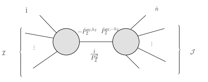
Figure 2: The amplitude is divided into a left set ${\cal I}\cup\hat{1}$ and a right set ${\cal J}\cup\hat{n}$. Note that here, as opposed to in figure 1, no ordering is inferred among the partons on the left and right side.

$$\widehat{P}_{\cal I}^{2}(z)=\left(\widehat{p}_{1}(z)+\sum\limits_{k\in{\cal I}}p_{k}\right)^{2}=0,$$ (29)

giving the poles

$$z_{\cal I}={\left(p_{1}+\sum\limits_{k\in{\cal I}}p_{k}\right)^{2}\over 2q\cdot\left(p_{1}+\sum\limits_{k\in{\cal I}}p_{k}\right)}.~{}~{}$$ (30)

The $n$-gluon color-dressed amplitude is factorized into two lower point on-shell amplitudes

$$\mathcal{M}(z)\stackrel{{\scriptstyle z\rightarrow z_{\cal I}}}{{\longrightarrow}}\sum\limits_{i_{\cal I},h_{\cal I}}\mathcal{M}\left(\widehat{g}_{1}(z_{\cal I}),\{{g_{k}}\mid_{k\in{\cal I}}\},-\widehat{P}^{i_{\cal I},h_{\cal I}}_{\cal I}(z_{\cal I})\right){i\over\widehat{P}^{2}_{\cal I}(z_{\cal I})}\mathcal{M}\left(\widehat{P}^{i_{\cal I},-h_{\cal I}}_{\cal I}(z_{\cal I}),\{{g_{l}}\mid_{l\in\cal J}\},\widehat{g}_{n}(z_{\cal I})\right),$$ (31)

where $i_{\cal I}$ and $h_{\cal I}$ are used to denote the color and helicity indices for the internal line. Then at $z_{\cal I}$

$${\mathcal{M}(z)\over z}{\stackrel{{\scriptstyle z\rightarrow z_{\cal I}}}{{\longrightarrow}}}\sum\limits_{{i_{\cal I}},h_{\cal I}}\mathcal{M}\left(\widehat{g}_{1}(z_{\cal I}),\{{g_{k}}\mid_{k\in{\cal I}}\},-\widehat{P}^{i_{\cal I},h_{\cal I}}_{\cal I}(z_{\cal I})\right){i\over z_{\cal I}\widehat{P}^{2}_{\cal I}(z_{\cal I})}\mathcal{M}\left(\widehat{P}^{i_{\cal I},-h_{\cal I}}_{\cal I}(z_{\cal I}),\{{g_{l}}\mid_{l\in{\cal J}}\},\widehat{g}_{n}(z_{\cal I})\right).$$ (32)

Considering the position of the pole in eq. (30), we have

$${\mathcal{M}(z)\over z}\stackrel{{\scriptstyle z\rightarrow z_{\cal I}}}{{\longrightarrow}}-\sum\limits_{i_{\cal I},h_{\cal I}}{i{\mathcal{M}\left(\widehat{g}_{1}(z_{\cal I}),\{{g_{k}}\mid_{k\in{\cal I}}\},-\widehat{P}_{\cal I}^{i_{\cal I},h_{\cal I}}(z_{\cal I})\right)\mathcal{M}\left(\widehat{P}^{i_{\cal I},-h_{\cal I}}_{\cal I}(z_{\cal I}),\{{g_{l}}\mid_{l\in{\cal J}}\},\widehat{g}_{n}(z_{\cal I})\right)\over P^{2}_{\cal I}}}{1\over z-z_{\cal I}},$$ (33)

where the denominator is the squared sum of the momenta of the external legs in the left set. Thus the residue for the division ${\cal I},{\cal J}$ is

$$\operatornamewithlimits{\text{Res}}_{z\rightarrow z_{\cal I}}{\mathcal{M}(z)\over z} = -\sum\limits_{i_{\cal I},h_{\cal I}}{\mathcal{M}\left(\widehat{g}_{1}(z_{\cal I}),\{{g_{k}}\mid_{k\in{\cal I}}\},-\widehat{P}^{i_{\cal I},h_{\cal I}}_{\cal I}(z_{\cal I})\right)}{i\over P^{2}_{\cal I}}{\mathcal{M}\left(\widehat{P}^{i_{\cal I},-h_{\cal I}}_{\cal I}(z_{\cal I}),\{{g_{l}}\mid_{l\in{\cal J}}\},\widehat{g}_{n}(z_{\cal I})\right)}.$$

The numerator here is a product of two on-shell sub-amplitudes with the momentum of gluon $g_{1}$ and $g_{n}$ shifted. To get the full amplitude, we should sum over all possible residues at all finite poles. The amplitude is then given by the following BCFW recursion relation

$$\mathcal{M}\left({g_{1}},{g_{2}},\dots,{g_{n}}\right)~{}~{}~{}$$ (35)

$$= \sum\limits_{\cal I}\sum\limits_{i_{\cal I},h_{\cal I}}{\mathcal{M}\left(\widehat{g}_{1}(z_{\cal I}),\{{g_{k}}\mid_{k\in{\cal I}}\},-\widehat{P}^{i_{\cal I},h_{\cal I}}_{\cal I}(z_{\cal I})\right)}{i\over P^{2}_{\cal I}}{\mathcal{M}\left(\widehat{P}^{i_{\cal I},-h_{\cal I}}_{\cal I}(z_{\cal I}),\{{g_{l}}\mid_{l\in{\cal J}}\},\widehat{g}_{n}(z_{\cal I})\right)}.$$

3.2 Kinematic recursion

When we calculate an $(n>3)$-gluon color-dressed amplitude for a given helicity configuration, the configurations with all helicities positive and all helicities except one positive have to vanish Berends:1987me . The first nontrivial configuration is the MHV configuration with two negative helicity gluons.

It is convenient to use the spinor helicity formalism Berends:1981rb ; Causmaecker:1981bg ; Kleiss:1985yh ; Xu:1986xb ; Gunion:1985vca to study amplitudes. In the spinor helicity formalism, one expresses external momenta $p^{\mu}_{i}$ by double spinors $(\lambda_{i})_{a}(\widetilde{\lambda}_{i})_{\dot{a}}$, where $(\lambda_{i})_{a}$ and $(\widetilde{\lambda}_{i})_{\dot{a}}$ are two-dimensional Weyl spinors. The polarization vectors are explicitly expressed as $\varepsilon^{\mu+}\sim-\sqrt{2}{{\mu_{a}\widetilde{\lambda}_{\dot{a}}}\over\left\langle\mu\mid\lambda\right\rangle}$ and $\varepsilon^{\mu-}\sim-\sqrt{2}{{\lambda_{a}\widetilde{\mu}_{\dot{a}}}\over\left[\widetilde{\lambda}\mid\widetilde{\mu}\right]}$, where the spinor products are defined by $\left\langle\lambda\mid\mu\right\rangle\equiv\epsilon^{ba}\lambda_{a}\mu_{b}$ and $\left[\widetilde{\lambda}\mid\widetilde{\mu}\right]\equiv\epsilon^{\dot{a}\dot{b}}\widetilde{\lambda}_{\dot{a}}\widetilde{\mu}_{\dot{b}}$, using $\mu$ and $\widetilde{\mu}$ to denote the reference spinors. The matrices $\epsilon^{ab}$ and $\epsilon^{\dot{a}\dot{b}}$ are given by

$$\epsilon^{ab}=\epsilon^{\dot{a}\dot{b}}=\left(\begin{array}[]{cc}0&1\\ -1&0\\ \end{array}\right).$$ (38)

In the spinor helicity formalism, all amplitudes are expressed by spinor products. The color-ordered MHV amplitude is given by the famous formula

$$A\left(1^{+},2^{+},\dots,i^{-},\dots,j^{-},\dots,n^{+}\right)=i{\left\langle i\mid j\right\rangle^{4}\over\left\langle 1\mid 2\right\rangle\left\langle 2\mid 3\right\rangle\dots\left\langle{n-1}\mid n\right\rangle\left\langle n\mid 1\right\rangle},~{}~{}$$ (39)

which was conjectured in Parke:1986gb and proven in Berends:1987me . When we consider the $\overline{\text{MHV}}$ amplitude where all helicities are flipped, we just (up to a factor $(-1)^{n}$) replace $\left\langle{}\mid{}\right\rangle$ by $\left[{}\mid{}\right]$

$$A\left(1^{-},2^{-},\dots,i^{+},\dots,j^{+},\dots,n^{-}\right)=(-1)^{n}i{\left[i\mid j\right]^{4}\over\left[1\mid 2\right]\left[2\mid 3\right]\dots\left[{n-1}\mid n\right]\left[n\mid 1\right]}.$$ (40)

Let us now consider the color-dressed MHV amplitude with $g_{1}$ and $g_{n}$ as negative helicity gluons. We can conveniently shift the momenta of $g_{1}$ and $g_{n}$ in the spinor helicity formalism

$$\lambda_{1}\rightarrow\lambda_{1},\;\;\;\widetilde{\lambda}_{1}\rightarrow\widetilde{\lambda}_{1}-z\widetilde{\lambda}_{n},$$

$$\widetilde{\lambda}_{n}\rightarrow\widetilde{\lambda}_{n},\;\;\;\lambda_{n}\rightarrow\lambda_{n}+z\lambda_{1}.$$ (41)

This is nothing but the spinor expression of the $(1,n)$-shift defined by eq. (26), as $p_{1}\sim\lambda_{1}\widetilde{\lambda}_{1}$, $p_{n}\sim\lambda_{n}\widetilde{\lambda}_{n}$, and $q\sim\lambda_{1}\widetilde{\lambda}_{n}$. The constraint equations, eqs. (25), forcing the momenta in eq. (26) to remain on-shell, are automatically satisfied in this spinor expression and the boundary contribution $\mathcal{B}$ vanishes, meaning that we can use the BCFW recursion for the color-dressed amplitude eq. (35) without any boundary correction.

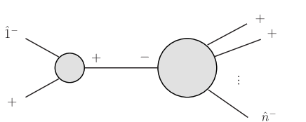
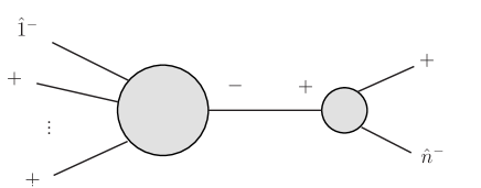
Figure 3: The allowed divisions, $(3,n-1)$ (left) and $(n-1,3)$ (right), for the MHV amplitude with the gluons with shifted momenta $\hat{1}$ and $\hat{n}$ as the negative helicity legs. As is proven in appendix A, only the $(n-1,3)$ factorization channel contributes.

We also note that with this shift, $g_{1}$ and $g_{n}$ must be in opposite sub-amplitudes. For MHV amplitudes, there are only two types of divisions, sketched in figure 3, which possibly could contribute

• The $(3,n-1)$ divisions with $3$-gluon $\overline{\text{MHV}}$ amplitudes as left sub-amplitudes and $(n-1)$-gluon MHV amplitudes as right sub-amplitudes.

• The $(n-1,3)$ divisions with $(n-1)$-gluon MHV amplitudes as left sub-amplitudes and $3$-gluon $\overline{\text{MHV}}$ amplitudes as right sub-amplitudes.

The other divisions always contain sub-amplitudes (for more than three gluons) with less than two negative helicity gluons and have to vanish. In fact, as is proven in appendix A, the $(3,n-1)$ division also vanishes. Thus the full color-dressed amplitude can be stated

$$\mathcal{M}\left(g_{1}^{-},g_{2}^{+},\cdots,g_{n-1}^{+},g_{n}^{-}\right)~{}~{}~{}~{}$$ (42)

$$= \sum\limits_{i=2}^{n-1}\mathcal{M}\left(\widehat{g}_{1}^{-},\dots,g_{i-1}^{+},\widehat{P}^{i_{i},-}_{i,n},g_{i+1}^{+},\dots,g^{+}_{n-1}\right){i\over P^{2}_{i,n}}\mathcal{M}\left(-\widehat{P}^{i_{i},+}_{i,n},g_{i}^{+},\widehat{g}_{n}^{-}\right),$$

where $i_{i}$ denotes the (implicitly summed over) color index connecting the sub-amplitudes. The right sub-amplitude is given by

$$\mathcal{M}\left(-\widehat{P}^{i_{i},+}_{i,n},g_{i}^{+},\widehat{g}_{n}^{-}\right)=g{1\over\sqrt{T_{R}}}if^{g_{i}i_{i}g_{n}}A^{\overline{\text{MHV}}}\left(i^{+},-\widehat{P}^{+}_{i,n},\widehat{n}^{-}\right)=g{1\over\sqrt{T_{R}}}if^{g_{i}i_{i}g_{n}}(-i){\left[i\mid-\widehat{P}_{i,n}\right]^{3}\over\left[-\widehat{P}_{i,n}\mid\widehat{n}\right]\left[\widehat{n}\mid i\right]}.\;\;\;$$ (43)

The left sub-amplitude is given by the $(n-1)$-gluon multiplet basis expansion

$$\mathcal{M}\left(\widehat{g}_{1}^{-},\dots,g_{i-1}^{+},\widehat{P}^{i_{i},-}_{i,n},g_{i+1}^{+},\dots,g_{n-1}^{+}\right)~{}~{}~{}$$ (44)

$$= g^{n-3}\sum\limits_{\alpha}\mathbf{V}^{\alpha}_{g_{1}\dots g_{i}\dots g_{n-1}}|_{g_{i}\rightarrow i_{i}}{A}^{\alpha}\left(\widehat{1}^{-},\dots,(i-1)^{+},\widehat{P}^{-}_{i,n},(i+1)^{+},\dots,(n-1)^{+}\right),$$

where, at this point, we make no statement about what gluons are counted as incoming and outgoing in the multiplet bases. The recursion relation between the $n$-gluon color factors and the $(n-1)$-gluon color factors can be written as

$$\left(\mathbf{V}^{\alpha}_{g_{1}\dots g_{i}\dots g_{n-1}}|_{g_{i}\rightarrow i_{i}}\right)if^{g_{i}i_{i}g_{n}} = \sum\limits_{\beta}\left(\mathbf{T}_{i}\right)_{\beta\alpha}\mathbf{V}^{\beta}_{g_{1}\dots g_{n}}.$$ (45)

The matrices $\mathbf{T}_{i}$ describe the effect of emitting gluon $n$ from gluon $i$ (from the vector $\alpha$ in the $(n-1)$-gluon basis), decomposed into the $n$-gluon basis. We will refer to these matrices as the radiation matrices for $(n-1)\rightarrow n$ gluons, and in section 3.3, we will show how to calculate them efficiently. Inserting eq. (44) and eq. (45) into the BCFW expression for the color-dressed amplitude, eq. (42), and collecting the kinematic factor corresponding to $\mathbf{V}^{\beta}_{g_{1}\dots g_{n}}$, we obtain the recursion relation for the kinematic factor in the MHV configuration

$${A}^{\beta}\left(1^{-},2^{+},3^{+},\dots,n^{-}\right)$$

$$= \sum\limits_{i=2}^{n-1}\sum\limits_{\alpha}\left(\mathbf{T}_{i}\right)_{\beta\alpha}\times\left[{A}^{\alpha}\left(\widehat{1}^{-},\dots,(i-1)^{+},\widehat{P}^{-}_{i,n},(i+1)^{+},\dots,(n-1)^{+}\right){i\over s_{i,n}}(-i){1\over\sqrt{T_{R}}}{\left[i\mid-\widehat{P}_{i,n}\right]^{3}\over\left[-\widehat{P}_{i,n}\mid\widehat{n}\right]\left[\widehat{n}\mid i\right]}\right],$$

where $s_{i,n}=(p_{i}+p_{n})^{2}=2p_{i}\cdot p_{n}$.

The above recursion relation for the kinematic factors expresses the kinematic factor of the $n$-gluon MHV amplitude in terms of the $(n-1)$-gluon MHV amplitude and the three-gluon $\overline{\text{MHV}}$ amplitude. To calculate the $n$-gluon kinematic factor for the MHV configuration using eq. (3.2), we thus use the kinematic factors in the multiplet basis expansion of the $(n-1)$-gluon MHV amplitude and the matrices ${\mathbf{T}_{i}}$ (which will be derived in the next section) as input.

3.3 Color structure recursion

Before stating expressions in the multiplet bases we need to fix our conventions. The vector space of interest is the overall singlet space for the involved (incoming plus outgoing) partons. Clearly the basis vectors for this space can be chosen in many different ways. The prescription detailed in Keppeler:2012ih constructs vectors by first constructing gluon projection operators projecting on irreducible representations for $\lfloor n/2\rfloor\rightarrow\lfloor n/2\rfloor$ gluons. Following this, basis vectors for processes with up to $n$ gluons can be constructed. (The extension to processes involving quarks is achieved by grouping the quarks and antiquarks to $q\overline{q}$-pairs and noting that each pair transforms either as a singlet or as an octet.) For a process with $n$ gluons, the gluons are divided into $\lceil n/2\rceil$ “incoming” gluons and $\lfloor n/2\rfloor$ “outgoing” gluons, such that there are either equally many outgoing and incoming gluons or one more incoming gluon. For the full set of gluons to transform under a singlet, the overall representation under which the “incoming” gluons transform must match the overall representation under which the “outgoing” gluons transform. The total dimension of the vector space is thus given by the number of ways of combining matching “incoming” and outgoing representations.

The gluons on either side are then subgrouped such that the first two gluons transform under representation $\alpha_{1}$, the first three gluons transform under representation $\alpha_{2}$, etc. The set of representations is collectively referred to as $\alpha$, and the “incoming” gluons are taken to be $g_{1},g_{3},...,g_{2\lceil\frac{n}{2}\rceil-1}$, whereas the “outgoing” are given even numbers $g_{2},g_{4},...,g_{2\lfloor\frac{n}{2}\rfloor}$. Using these conventions, and letting single lines denote the adjoint representation and double lines denote arbitrary representations, the orthonormal basis vectors are

$$\mathbf{V}^{\alpha}_{g_{1}\,g_{3}\,\dots\,g_{2\lceil{n\over 2}\rceil-1};\,g_{2}\,g_{4}\,\dots\,g_{2\lfloor{n\over 2}\rfloor}} = N^{\alpha_{1}\dots\alpha_{n-3}}$$

$$\times \raisebox{-0.4pt}{ \includegraphics[width=354.12144pt]{figures/MultipletBasisVector} },$$

where

$$N^{\alpha_{1}\,\alpha_{2}\dots\alpha_{n-3}}=\sqrt{\frac{\prod_{i=1}^{n-3}{d_{\alpha_{i}}}}{\raisebox{-0.5pt}{\includegraphics[scale={0.3}]{figures/Wig3jBasisVector/Wig3j_1}}\raisebox{-0.4pt}{\includegraphics[scale={0.3}]{figures/Wig3jBasisVector/Wig3j_2}}\dots\raisebox{-0.43pt}{\includegraphics[scale={0.3}]{figures/Wig3jBasisVector/Wig3j_nM2}}\raisebox{-0.43pt}{\includegraphics[scale={0.3}]{figures/Wig3jBasisVector/Wig3j_nM1}}\dots\raisebox{-0.4pt}{\includegraphics[scale={0.3}]{figures/Wig3jBasisVector/Wig3j_nM4}}\raisebox{-0.5pt}{\includegraphics[scale={0.3}]{figures/Wig3jBasisVector/Wig3j_nM3}}}}.$$ (48)

Here the vacuum bubbles in the denominator are Wigner $3j$ coefficients. They can be normalized to one, inducing a normalization for the generalized vertices connecting the representations.

Letting $A^{\alpha}(1,2,\dots,n)$ denote the amplitude (for convenience we keep the gluon arguments in $A^{\alpha}$ in this order) the decomposition into these bases may thus be written

$${\cal M}(g_{1},g_{2},\dots,g_{n})=g^{n-2}\sum\limits_{\alpha}\mathbf{V}^{\alpha}_{g_{1}\,g_{3}\,...g_{2\lceil\frac{n}{2}\rceil-1};\,g_{2}\,g_{4}\,...g_{2\lfloor\frac{n}{2}\rfloor}}A^{\alpha}(1,2,\dots,n).~{}~{}$$ (49)

A remark on the implication of charge conjugation is in place. As gluons transform under the charge conjugation invariant adjoint representation, any overall gluon amplitude must respect this symmetry. This is manifest in the DDM bases in the sense that each spanning color structure obeys this symmetry, but it is not manifest in the trace bases and the multiplet bases. For tree-level trace bases charge conjugation invariance instead shows up as cyclic reflection. For multiplet bases, charge conjugation invariance displays itself by the amplitude for a (non-invariant) basis vector and its conjugate being equal up to a sign – and by the vanishing of amplitudes for which all involved representations are invariant, but the invariance is spoiled by the generalized vertices.

For many gluons almost all of the basis vectors contain at least one representation which is not charge conjugation invariant, meaning that almost every basis vector must occur with its conjugate. Using these linear combinations as basis vectors thus reduces the dimension of the vector space by approximately a factor two.

For the explicit calculations for four, five and six gluons, we have used conjugation invariant bases. However, for comparison, the dimensions of the vector spaces, are – as for the trace basis case – stated without this symmetry in table 1. This also has the advantage that the vector space dimension for $n$ gluons is approximately equal to the dimension for $n-n_{q}$ gluons and $n_{q}$ $q\overline{q}$-pairs, see Sjodahl:2015qoa .

With the above basis conventions the radiation matrices, eq. (45), are given by

$$\left(\mathbf{V}^{\alpha}_{g_{1}\,g_{3}\,\dots\,g_{2\lceil{n-1\over 2}\rceil-1};\,g_{2}\,g_{4}\,\dots\,g_{2\lfloor{n-1\over 2}\rfloor}}\Big{|}_{g_{i}\rightarrow i_{i}}\right)if^{g_{i}i_{i}g_{n}}=\sum_{\beta}{\left(\mathbf{T}_{i}\right)_{\beta\alpha}\mathbf{V}^{\beta}_{g_{1}\,g_{3}\,\dots\,g_{2\lceil{n\over 2}\rceil-1};\,g_{2}\,g_{4}\,\dots\,g_{2\lfloor{n\over 2}\rfloor}}},$$ (50)

giving for the amplitudes, eq. (3.2),

$${A}^{\beta}\left(1^{-},2^{+},3^{+},\dots,n^{-}\right)=\sum\limits_{i=2}^{n-1}\sum\limits_{\alpha}\left(\mathbf{T}_{i}\right)_{\beta\alpha}$$

$$\times\left[{A}^{\alpha}\left(\widehat{1}^{-},2^{+},\dots,(i-1)^{+},\widehat{P}^{-}_{i,n},(i+1)^{+},\dots,(n-1)^{+}\right){1\over s_{i,n}}{1\over\sqrt{T_{R}}}{\left[i\mid-\widehat{P}_{i,n}\right]^{3}\over\left[-\widehat{P}_{i,n}\mid\widehat{n}\right]\left[\widehat{n}\mid i\right]}\right].$$ (51)

As can be seen in eq. (50), the color structure of the recursion relation in the multiplet bases is given by inserting one gluon to the $(n-1)$-gluon basis vectors,

$$\left(\mathbf{V}^{\alpha}_{g_{1}\,g_{3}\,\dots\,g_{2\lceil{n-1\over 2}\rceil-1};\,g_{2}\,g_{4}\,\dots\,g_{2\lfloor{n-1\over 2}\rfloor}}\Big{|}_{g_{i}\rightarrow i_{i}}\right)if^{g_{i}i_{i}g_{n}}.$$ (52)

For example, denoting the five-gluon basis vectors $\mathbf{V}^{\alpha}_{g_{1}\,g_{3}\,g_{5};\,g_{2}\,g_{4}}$, if we radiate another gluon $g_{6}$, we can attach it to any of the gluons $g_{1}$, $g_{2}$, $g_{3}$, $g_{4}$ and $g_{5}$. The corresponding color factors then become $\mathbf{V}^{\alpha}_{i\,g_{3}\,g_{5};\,g_{2}\,g_{4}}if^{g_{1}ig_{6}}$, $\mathbf{V}^{\alpha}_{g_{1}\,g_{3}\,g_{5};\,i\,g_{4}}if^{g_{2}ig_{6}}$, $\mathbf{V}^{\alpha}_{g_{1}\,i\,g_{5};\,g_{2}\,g_{4}}if^{g_{3}ig_{6}}$, $\mathbf{V}^{\alpha}_{g_{1}\,g_{3}\,g_{5};\,g_{2}\,i}if^{g_{4}ig_{6}}$ and $\mathbf{V}^{\alpha}_{g_{1}\,g_{3}\,i;\,g_{2}\,g_{4}}if^{g_{5}ig_{6}}$. The systematic evaluation of such color structure in the larger basis is the topic of the present section.

One way of evaluating the radiation matrices is to simply calculate scalar products between the left hand side color structure of eq. (50) and the vectors in the larger basis. This is equivalent to the method of section 2. However, as most of these scalar products vanish – for reasons that will become clear later in this section – such a strategy would be unnecessarily expensive.

Instead we here present a more elegant way of evaluating the weights for the $n$-gluon basis vectors using group theory and the birdtrack notation Cvi08 . By applying group theoretical relations to the left hand side of eq. (50) it can be cast into the form of the right hand side, with the radiation matrix elements expressed in terms of group theoretical weights, the Wigner coefficients.

A method for evaluating scalar products between Feynman diagrams and multiplet basis vectors is explored in Sjodahl:2015qoa . The same techniques are applicable for the decomposition of an $(n-1)$-gluon multiplet basis vector which has radiated an $n$th gluon, into $n$-gluon multiplet basis vectors. For this decomposition, three group theoretical relations are required, the completeness relation for tensor products, the color structure of a vertex correction and the relation between the ordering of the representations of a vertex. In birdtrack notation the completeness relation reads

$$\raisebox{-0.325pt}{ \includegraphics[scale={0.45}]{figures/CompletenessRelation/CR_LHS} }=\sum_{\alpha\in{}\mu\otimes\nu}{\frac{d_{\alpha}}{\includegraphics[scale={0.3}]{figures/CompletenessRelation/Wig3jMuAlphaNu}}\raisebox{-0.325pt}{ \includegraphics[scale={0.45}]{figures/CompletenessRelation/CR_RHS} }}.$$ (53)

In the tensor product $\mu\otimes\nu$ above, there can be more than one instance of a particular representation. In this case all instances have to be summed over, for example in $A\otimes A$, where $A$ denotes the adjoint representation (not to be confused with the amplitude), there are two “octets”.

The second relation is a special case of the Wigner-Eckart theorem, the color structure of a vertex correction can be written as Sjodahl:2015qoa ; Cvi08

$$\raisebox{-0.44pt}{ \includegraphics[scale={0.45}]{figures/RadiationMatrix/VertexCorrection/VertexCorrection} }=\sum_{a}{\frac{\raisebox{-0.45pt}{ \includegraphics[scale={0.45}]{figures/RadiationMatrix/VertexCorrection/Wig6j} }}{\raisebox{-0.45pt}{ \includegraphics[scale={0.3}]{figures/RadiationMatrix/VertexCorrection/Wig3j} }}\raisebox{-0.43pt}{ \includegraphics[scale={0.45}]{figures/RadiationMatrix/VertexCorrection/Vertex} }}.$$ (54)

The above equation is sometimes stated without the sum. Indeed the sum is only needed if there is more than one instance of $\gamma$ in the tensor product $\alpha\otimes\beta$. In this case, the $\alpha\beta\gamma$-vertex may appear in more than one version, this occurs, for example, when $\alpha$, $\beta$ and $\gamma$ are octets, then $a$ is $if$ and $d$.

The third relation concerns the ordering of representations in a vertex, the relation between the two orderings is given by Cvi08 ,

$$\raisebox{-0.41pt}{ \includegraphics[scale={0.45}]{figures/RadiationMatrix/YutsisVertex/VertexYutsis} }\equiv\raisebox{-0.41pt}{ \includegraphics[scale={0.45}]{figures/RadiationMatrix/YutsisVertex/VertexInitialOrder} }=\sum_{a}{\frac{\raisebox{-0.45pt}{ \includegraphics[scale={0.3}]{figures/RadiationMatrix/YutsisVertex/Wig3jYutsis} }}{\raisebox{-0.45pt}{ \includegraphics[scale={0.3}]{figures/RadiationMatrix/YutsisVertex/Wig3j} }}\raisebox{-0.43pt}{ \includegraphics[scale={0.45}]{figures/RadiationMatrix/YutsisVertex/VertexNormal} }},$$ (55)

where the equivalence defines Yutsis’ notation YutsisNotation . Typically this just gives a sign $\pm 1$, for example we have a minus sign for the antisymmetric triple-gluon vertex.

3.3.1 Example: $4\rightarrow 5$ gluons

The method of evaluating the radiation matrices with the above stated relations will first be applied to a $4\rightarrow 5$ gluon example, and after that a general formula will be derived. Let us thus consider a four-gluon basis vector radiating a fifth gluon from gluon 3. In diagrammatic form, denoting the standard triple gluon vertex, $if^{abc}$, with a black dot, where the indices are read in counter clockwise order, the color structure becomes

$$N^{\alpha_{1}}\raisebox{-0.45pt}{ \includegraphics[scale={0.5}]{figures/RadiationMatrix/Example/InitialColorStructure} },$$ (56)

where we have drawn the fifth gluon such that the gluon ordering in eq. (3.3) is respected.

Applying the completeness relation eq. (53) to gluon 5 and the representation $\alpha_{1}$ gives

$$N^{\alpha_{1}}\raisebox{-0.45pt}{ \includegraphics[scale={0.45}]{figures/RadiationMatrix/Example/InitialColorStructure} }=-\sum_{\beta_{1}\in{}A\otimes\alpha_{1}}{\frac{d_{\beta_{1}}}{\includegraphics[scale={0.3}]{figures/RadiationMatrix/Example/Wig3jCR}}N^{\alpha_{1}}\raisebox{-0.45pt}{ \includegraphics[scale={0.45}]{figures/RadiationMatrix/Example/CRAppliedColorStructure} }},$$ (57)

where the sum runs over representations in the adjoint representation times $\alpha_{1}$. On the right hand side above, gluon 1 and 3 and the representation $\beta_{1}$ are connected by a vertex correction. Using eq. (54) with $\gamma\rightarrow\beta_{1}$, $\epsilon\rightarrow\alpha_{1}$ and $\alpha,\beta,\delta,\zeta\rightarrow{}A$ to remove it, the color structure is

$$N^{\alpha_{1}}\raisebox{-0.45pt}{ \includegraphics[scale={0.45}]{figures/RadiationMatrix/Example/InitialColorStructure} }=-\sum_{\begin{subarray}{c}\beta_{1}\in{}(A\otimes\alpha_{1}\cap A\otimes{}A)\\ a\end{subarray}}{\frac{d_{\beta_{1}}}{\includegraphics[scale={0.3}]{figures/RadiationMatrix/Example/Wig3jCR}}\frac{\raisebox{-0.25pt}{ \includegraphics[scale={0.45}]{figures/RadiationMatrix/Example/Wig6j} }}{\includegraphics[scale={0.3}]{figures/RadiationMatrix/Example/Wig3jVertexCorrection}}\frac{N^{\alpha_{1}}}{N^{\beta_{1}\alpha_{1}}}N^{\beta_{1}\alpha_{1}}\raisebox{-0.45pt}{ \includegraphics[scale={0.45}]{figures/RadiationMatrix/Example/FinalColorStructure} }}.$$ (58)

This equation is now of the desired form, eq. (50) where the radiation matrix components trivially can be read off by comparison to eq. (3.3). Letting $\beta=(\beta_{1},\beta_{2})$ denote the representation set labeling the $5$-gluon basis vector, we immediately see that the representation $\beta_{2}$ is constrained to be $\beta_{2}=\alpha_{1}$. Thus most of the projections onto the $5$-gluon basis vectors vanish.

Note that eq. (58) has been derived without explicitly stating the representation $\alpha_{1}$. The result is thus generic and, knowing the Wigner coefficients and the dimensions of the representations, it can be used for immediately writing down the decomposition for any initial $\mathbf{V}^{\alpha}$. As an example, if $\alpha_{1}=10$ the allowed $\beta_{1}$ representations, i.e., those present in both $A\otimes\alpha_{1}$ and $A\otimes{}A$, are 8, 10, 27 and 0 (for $N_{c}\geq 4$). If $\beta_{1}=8$, there are two possible vertices connecting gluon 1 and 3 in the 5-gluon basis vector, and similarly if $\beta_{1}=10$ (and $N_{c}\geq 4$) there are two vertices connecting $\beta_{1}$ and $\alpha_{1}$.

For evaluating the right hand side of eq. (58) we use the dimensions of the representations, stated in eq. (22), and the Wigner coefficients calculated as in Sjodahl:2015qoa . Ordering the allowed representations $\beta_{1}$ as $(8^{s}$, $8^{a}$, $27$, $10^{f}$, $10^{fd},0)$, the Wigner $6j$ coefficient in eq. (58) takes the values

$$\left(\frac{-1}{\sqrt{N_{c}^{2}-4}\left(N_{c}^{2}-1\right)},0,\frac{1}{\sqrt{N_{c}^{2}+3N_{c}+2}\left(N_{c}^{2}-N_{c}\right)},\frac{\sqrt{2}}{\sqrt{N_{c}^{2}-4}\left(N_{c}^{2}-1\right)},0,\frac{1}{\sqrt{N_{c}^{2}-3N_{c}+2}\left(N_{c}^{2}+N_{c}\right)}\right)$$ (59)

respectively. In Sjodahl:2015qoa the Wigner $3j$ coefficients are normalized to one. Eq. (58) is valid for any normalization as long as it is consistently used. However, requiring all $3j$ coefficient to be one implies a normalization $i\tilde{f}^{abc}i\tilde{f}^{cba}=1$ for the triple-gluon vertex. To get the correct $if^{abc}$-normalization, eq. (59) must be therefore multiplied by a factor of

$$\sqrt{\raisebox{-0.4pt}{ \includegraphics[scale={0.3}]{figures/RadiationMatrix/Example/Wig3jStructureConstant} }}=\sqrt{2N_{c}(N_{c}^{2}-1)T_{R}}\;\;\mbox{ (using standard normalization of vertices)}.$$ (60)

Normalizing the Wigner $3j$ coefficients to one and using the definition of the normalization constants, eq. (48), gives

$$\frac{N^{\alpha_{1}}}{N^{\beta_{1}\alpha_{1}}}=\frac{1}{\sqrt{d_{\beta_{1}}}}.$$ (61)

Combining the dimensions, the Wigner $6j$ coefficients, the normalization factor eq. (60), and the overall sign in eq. (58) gives

$$\sqrt{T_{R}}\left(\sqrt{\frac{2N_{c}}{N_{c}^{2}-4}},0,-\sqrt{\frac{N_{c}(N_{c}+3)}{2(N_{c}+2)}},-\sqrt{N_{c}},0,-\sqrt{\frac{N_{c}(N_{c}-3)}{2(N_{c}-2)}}\right).$$ (62)

These are the factors required to express the color structure of eq. (56) in terms of the five-gluon basis vectors. For bases which are not charge conjugation invariant, they would be the entries in the radiation matrix $\mathbf{T}_{3}$, corresponding to mapping the initial vector $\mathbf{V}^{10}$ emitting a gluon $g_{5}$ from gluon $g_{3}$ onto the five-gluon basis vectors $\mathbf{V}^{8s,10}$, $\mathbf{V}^{8a,10}$, $\mathbf{V}^{27,10}$, $\mathbf{V}^{10,10f}$, $\mathbf{V}^{10,10fd}$ and $\mathbf{V}^{10,0}$. In the above case, the initial color structure, eq. (56) with $\alpha_{1}=10$, is from a basis vector which is not charge conjugation invariant, and neither is any of the vectors which the color structure is projected onto. To get to the charge conjugation invariant vectors in this case simply requires the substitution of $10\rightarrow 20$ in the vector representation labels. With this change, the result, eq. (62), can be compared to column five of $\mathbf{T}_{3}$ in eq. (124) in appendix B, where the radiation matrices for $4\rightarrow 5$ gluons are given expressed in the basis from eq. (B) (which is also electronically attached as an online resource).

In general, when knowing the radiation matrices in non-charge conjugation invariant bases and converting to charge conjugation invariant bases, a sign might be required since the $n$-gluon non-invariant vector may come with a minus sign in the linear combination building up the charge conjugation invariant vector. For the same reason another minus sign may come from the $(n-1)$-gluon basis vector. Apart from a potential sign, factors compensating for vector normalizations and occurrence of both a vector and its conjugate on the right hand side of eq. (50) may be required.

For five external gluons (and $N_{c}\geq 4$) there are 22 charge conjugation invariant basis vectors, stated in eq. (B), but the example color structure is given by only four of them. It is worth noting that although, in this case, most of the basis vectors with $\beta_{2}=10$ contribute (there are only two zeros in eq. (62)), for more external gluons the constraints corresponding to $\beta_{1}\in{}\alpha_{1}\otimes{}A$ become more restrictive. This point will be elaborated on after the derivation of the general formula for radiation matrices.

3.3.2 The general case: $n-1\rightarrow n$ gluons

In general, if the $n$th gluon is radiated from one of the incoming gluons, the color structure of eq. (52) will be of the form

$$N^{\alpha_{1}\,\alpha_{2}\dots\alpha_{n-1-3}}\raisebox{-0.45pt}{ \includegraphics[scale={0.6}]{figures/RadiationMatrix/GeneralCase/InitialColorStructure} },$$ (63)

where, if $j=0$ or 1 (i.e. $i=1$ or 3), $\alpha_{j-1}$ is an octet. In the following steps it will be assumed that gluon 1 is not the emitter, this special case will be addressed after the derivation. To get to the right hand side of eq. (50), the same steps as in the above example are used: First the completeness relation, eq. (53), is applied repeatedly and then vertex corrections are removed using eq. (54).

We thus want to apply the completeness relations to gluon $n$ and the representations $\alpha_{j},\alpha_{j+1},\dots,\alpha_{\lceil\frac{n-1}{2}\rceil-1}$, i.e., we insert it in the encircled positions in

$$N^{\alpha_{1}\,\alpha_{2}\dots\alpha_{n-4}}\raisebox{-0.45pt}{ \includegraphics[scale={0.6}]{figures/RadiationMatrix/GeneralCase/CRPlacementsColorStructure} },$$ (64)

resulting in

$$\sum_{\beta_{j},\beta_{j+1},\dots,\beta_{\lceil\frac{n-1}{2}\rceil-1}}{\frac{d_{\beta_{j}}}{\raisebox{-0.45pt}{ \includegraphics[scale={0.3}]{figures/RadiationMatrix/GeneralCase/Wig3j/Wig3j_j}}}\frac{d_{\beta_{j+1}}}{\raisebox{-0.45pt}{ \includegraphics[scale={0.3}]{figures/RadiationMatrix/GeneralCase/Wig3j/Wig3j_jP1}}}\dots\frac{d_{\beta_{\lceil\frac{n-1}{2}\rceil-1}}}{\raisebox{-0.45pt}{ \includegraphics[scale={0.3}]{figures/RadiationMatrix/GeneralCase/Wig3j/Wig3j_CeilnM1M1}}}N^{\alpha_{1}\,\alpha_{2}\dots\alpha_{n-4}}}$$

$$\times\raisebox{-0.45pt}{ \includegraphics[scale={0.6}]{figures/RadiationMatrix/GeneralCase/CRAppliedColorStructure} }.$$ (65)

Here gluon $2j+1$ has a vertex correction of a different form compared to the other gluons. We first treat this separately and then address all other vertex corrections. Using Yutsis’ notation, eq. (55), and eq. (54), the leftmost vertex correction can be written

$$\raisebox{-0.45pt}{ \includegraphics[scale={0.6}]{figures/RadiationMatrix/GeneralCase/VertexCorrection/VertexCorrection_Leg2jP1} }=\sum_{b_{j}}{\hskip 8.53581pt\frac{\raisebox{-0.45pt}{ \includegraphics[scale={0.45}]{figures/RadiationMatrix/GeneralCase/VertexCorrection/Wig6j_Leg2jP1} }}{\raisebox{-0.45pt}{ \includegraphics[scale={0.3}]{figures/RadiationMatrix/GeneralCase/VertexCorrection/Wig3j_Leg2jP1} }}\raisebox{-0.45pt}{ \includegraphics[scale={0.6}]{figures/RadiationMatrix/GeneralCase/VertexCorrection/Vertex_j} }}.$$ (66)

The remaining vertex corrections can be contracted similarly, for example

$$\raisebox{-0.45pt}{ \includegraphics[scale={0.6}]{figures/RadiationMatrix/GeneralCase/VertexCorrection} }=\sum_{b_{j+1}}{\frac{\hskip 2.84526pt\raisebox{-0.45pt}{ \includegraphics[scale={0.45}]{figures/RadiationMatrix/GeneralCase/VertexCorrection/Wig6j_FirstVC} }}{\raisebox{-0.45pt}{ \includegraphics[scale={0.3}]{figures/RadiationMatrix/GeneralCase/VertexCorrection/Wig3j_FirstVC} }}\raisebox{-0.45pt}{ \includegraphics[scale={0.6}]{figures/RadiationMatrix/GeneralCase/VertexCorrection/Vertex_jP1} }}.$$ (67)

Applying the above steps and adjusting the vertex order of the last new vertex results in

$$\sum_{\begin{subarray}{c}\beta_{j},\beta_{j+1},\dots,\beta_{\lceil\frac{n-1}{2}\rceil-1}\\ b_{j},b_{j+1},\dots,b_{\lceil\frac{n-1}{2}\rceil}\end{subarray}}{\frac{d_{\beta_{j}}}{\raisebox{-0.45pt}{ \includegraphics[scale={0.3}]{figures/RadiationMatrix/GeneralCase/Wig3j/Wig3j_j} }}\frac{\raisebox{-0.25pt}{ \includegraphics[scale={0.4}]{figures/RadiationMatrix/GeneralCase/VertexCorrection/Wig6j_Leg2jP1} }}{\raisebox{-0.3pt}{ \includegraphics[scale={0.3}]{figures/RadiationMatrix/GeneralCase/VertexCorrection/Wig3j_Leg2jP1} }}\left[\prod_{k=j+1}^{\lceil\frac{n-1}{2}\rceil{-1}}{\frac{d_{\beta_{k}}}{\raisebox{-0.45pt}{ \includegraphics[scale={0.3}]{figures/RadiationMatrix/GeneralCase/VertexCorrection/GeneralLeg/Wig3j_Leg2kP1_CR} }}\frac{\raisebox{-0.25pt}{ \includegraphics[scale={0.4}]{figures/RadiationMatrix/GeneralCase/VertexCorrection/GeneralLeg/Wig6j_Leg2kP1} }}{\raisebox{-0.3pt}{ \includegraphics[scale={0.3}]{figures/RadiationMatrix/GeneralCase/VertexCorrection/GeneralLeg/Wig3j_Leg2kP1} }}}\right]\frac{\raisebox{-0.1pt}{ \includegraphics[scale={0.3}]{figures/RadiationMatrix/GeneralCase/Wig3jYutsis} }}{\hskip 2.84526pt\raisebox{-0.3pt}{ \includegraphics[scale={0.3}]{figures/RadiationMatrix/GeneralCase/Wig3jYutsisNorm} }}}$$

$$\times\frac{N^{\alpha_{1}\,\alpha_{2}\dots\alpha_{n-4}}}{N^{\alpha_{1}\dots\alpha_{j-1}\beta_{j}\dots\beta_{\lceil\frac{n-1}{2}\rceil{-1}}\,\alpha_{\lceil\frac{n-1}{2}\rceil{-1}}\dots\alpha_{n-4}}}N^{\alpha_{1}\dots\alpha_{j-1}\beta_{j}\dots\beta_{\lceil\frac{n-1}{2}\rceil{-1}}\,\alpha_{\lceil\frac{n-1}{2}\rceil{-1}}\dots\alpha_{n-4}}$$

$$\times\raisebox{-0.45pt}{ \includegraphics[scale={0.6}]{figures/RadiationMatrix/GeneralCase/FinalColorStructure} },$$ (68)

where the vertex labels in the third line have been suppressed. The third line of eq. (68), combined with the last normalization factor of the second line is now of the form of a basis vector. Hence the factor in front of it is the radiation matrix $\mathbf{T}_{2j+1}$ expressed in terms of Wigner coefficients.

We remark that the form of the radiation matrix from the example, eq. (58), differs from eq. (68). This is only due to the fifth gluon being drawn in an, at that point, more natural way. The two expressions are identical, if the expression from eq. (68) is written out for gluon 3 with $n=5$, it can be simplified to become exactly the expression of eq. (58).

The derived result, eq. (68), is for gluons emitted from the “incoming” gluons. For gluons emitted from the “outgoing” gluons an analogous derivation can be done, resulting in an equation similar to eq. (68). A special case occurs if the emitter is the first gluon on its side, gluon 1 for the “incoming” side and gluon 2 for the “outgoing” side. Compared to the radiation matrices $\mathbf{T}_{3}$ and $\mathbf{T}_{4}$ the matrices $\mathbf{T}_{1}$ and $\mathbf{T}_{2}$ are identical up to sign differences for some entries. The difference originates from a difference in the leftmost (rightmost for gluon 2) vertex correction, eq. (66), that results in a change in vertex ordering which gives a possible sign difference. (Taking gluon $1$ and gluon $n$ to be the gluons with shifted momenta, emission from gluon 1 need not be considered, see figure 3.)

Concerning the group theoretical constraints on the representations we note that each representation to the left of $\beta_{j}$ and to the right of $\beta_{\lceil\frac{n-1}{2}\rceil-1}$ are constrained to be equivalent to representations in the set $\alpha$, i.e.,

$$\beta_{k} = \alpha_{k},\;\;\;\;\mathrm{for}\;k=1,\dots,j-1,$$

$$\beta_{k} = \alpha_{k-1},\;\mathrm{for}\;k=\lceil\frac{n-1}{2}\rceil,\dots,n-3.$$ (69)

The shift in the index of the second equality in eq. (69) is from the fact that there are $n-3$ representations for $n$ gluons and $n-4$ for $n-1$ gluons, with the new representation being inserted just before $\alpha_{\lceil\frac{n-1}{2}\rceil-1}$.

There are also constraints on the set of representations $\beta$ coming from the completeness relations applied in eq. (65),

$$\beta_{k}\in{}\alpha_{k}\otimes{}A,\;\mathrm{for}\;k=j,j+1,\dots,\lceil\frac{n-1}{2}\rceil-1.$$ (70)

This constraint will become more restrictive when the emitting gluon is far from the middle of the basis vector, since in this case, the constraint is imposed on many representations in the basis vector.

Using the constraints eq. (69) and eq. (70), the number of possibly non-zero elements in the radiation matrix columns can be counted (more are zero due to generalized vertices giving Wigner coefficients which are zero). The result, averaged over all possible emitters $2,..,n-1$ and all possible initial basis vectors, is shown in table 1 along with the maximal number of possible $\beta$ for any $\alpha$. Both the maximal number of possible $\beta$ for any $\alpha$ and the average over all $\alpha$ and all emitters are overestimates, as symmetries of the Wigner coefficients will force some of them to vanish, depending on the choice of vertices. In addition, there are Wigner coefficients vanishing due to the invariance condition of tensors under the group, see Cvi08 for the invariance condition in birdtrack notation. For the calculated radiation matrices, the reductions due to vanishing Wigner coefficients changes the averages for $N_{c}\geq{}n$ from $6.9$ to $3.9$ and $14.4$ to $8.9$ for the $n=5$ and $n=6$ cases, respectively. For the gluons only case there is the further reduction due to charge conjugation invariance. For comparison, table 1 also shows the dimensions of the (all order) vector space, both for QCD and in the limit $N_{c}\rightarrow\infty$, and the number of vectors in the spanning sets for the “trace bases” and “DDM bases”.

	$n$	5	$6$	$7$	$8$	$9$	$10$	$11$	$12$
Avg	QCD	6.0	10.8	17.5	32.5	54.6	106	185	268
	$N_{c}\geq{}n$	6.9	14.4	24.6	57.9	109	299	593	1 775
Max	QCD	8	33	33	178	178	962	962	5 220
	$N_{c}\geq{}n$	9	44	44	400	400	4 006	4 006	41 256
Vectors	QCD	32	145	702	3 598	19 280	107 160	614 000	3 609 760
(all orders)	$N_{c}\geq{}n$	44	265	1 854	14 833	133 496	1 334 961	14 684 570	176 214 841
Trace	any $N_{c}$	24	120	720	5 040	40 320	362 880	3 628 800	39 916 800
DDM	any $N_{c}$	6	24	120	720	5 040	40 320	362 880	3 628 800

Table 1: The average (taken over all initial vectors and the emitters $2,...,n-1$) and maximal number of non-zero elements in the columns of the radiation matrices for $(n-1)\rightarrow n$ gluons. The stated numbers are overestimates since they assume that no Wigner $6j$ coefficient involving admissible representations vanishes. For comparison we also show the total dimension of the all order vector space for $N_{c}\geq n$ and for $N_{c}=3$ (without accounting for reduction due to charge conjugation invariance) and the number of spanning vectors in the tree-level trace bases and the DDM bases.

We note that although the average (and maximal) number of terms does increase with the number of gluons, compared to the increase in the dimension of the vector space, this growth is very mild, meaning that a smaller and smaller fraction of all basis vectors contribute. Instead of having to treat the square of the number of basis vectors in the squaring of the amplitude, we thus only need to treat the number of basis vectors, times the number of contributing emitters times the average number of terms in deriving the amplitude; recall that the squaring of the color structure itself is quick in the orthogonal bases. For example, using the trace basis for 10 gluons requires $(362\,880)^{2}\sim 10^{11}$ terms in the squaring step, with the (gluon specific) DDM basis this can be reduced to $\sim 10^{9}$, whereas using the multiplet basis would require up to $19\,208\times 8\times 106\sim 10^{7}$ terms for the identification of new basis vectors. For more gluons the difference is even larger. As our long term goal is to include processes with an arbitrary number of quarks, we view the comparison between the non charge conjugation invariant multiplet basis and the trace basis as the most relevant comparison. From table 1 we thus conclude that the overall treatment of the color structure can be sped up significantly by the usage of multiplet bases.

3.4 The five-gluon amplitude

Utilizing that only the $(n-1,3)$ division contributes, the BCFW recursion expression, eq. (42), for the five-gluon color-dressed MHV amplitude is given by the sum of the diagrams in figure 4. As seen in eq. (2.2), the four-gluon color-dressed (MHV) sub-amplitudes can be expressed in the multiplet basis.

The contractions of basis vectors in the four-gluon sub-amplitudes and the structure constants in the three-gluon sub-amplitudes can be expanded in the five-gluon multiplet basis using the radiation matrices $\mathbf{T}_{i}$ for emitting the gluon $g_{5}$, illustrated in figure 4. Collecting the kinematic factors corresponding to a given five-gluon basis vector, we can write down the recursion relation eq. (3.3) for the kinematic factor for five gluons

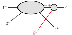
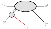
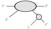
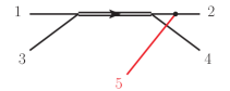
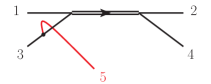
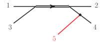
Figure 4: The relevant splittings for the BCFW recursion in the five-gluon MHV case (above) and the corresponding color structure for the radiation matrices (below). Note that the orders of the $if^{g_{i}g_{i,n}g_{n}}$ vertices are drawn to be consistent with eq. (3.3).

$${A}^{\beta}({1^{-},2^{+},3^{+},4^{+},5^{-}}) = ~{}~{}\sum\limits_{\alpha}\left(\mathbf{T}_{2}\right)_{\beta\alpha}{A}^{\alpha}\left(\widehat{1}^{-},\widehat{P}^{-}_{2,5},3^{+},4^{+}\right){1\over s_{25}}{1\over\sqrt{T_{R}}}{\left[2\mid-\widehat{P}_{2,5}\right]^{3}\over\left[2\mid\widehat{5}\right]\left[\widehat{5}\mid-\widehat{P}_{2,5}\right]}$$ (71)

$$+\sum\limits_{\alpha}\left(\mathbf{T}_{3}\right)_{\beta\alpha}{A}^{\alpha}\left({\widehat{1}^{-},2^{+},\widehat{P}^{-}_{3,5},4^{+}}\right){1\over s_{35}}{1\over\sqrt{T_{R}}}{\left[3\mid-\widehat{P}_{3,5}\right]^{3}\over\left[3\mid\widehat{5}\right]\left[\widehat{5}\mid-\widehat{P}_{3,5}\right]}$$

$$+\sum\limits_{\alpha}\left(\mathbf{T}_{4}\right)_{\beta\alpha}{A}^{\alpha}\left(\widehat{1}^{-},2^{+},3^{+},\widehat{P}^{-}_{4,5}\right){1\over s_{45}}{1\over\sqrt{T_{R}}}{\left[4\mid-\widehat{P}_{4,5}\right]^{3}\over\left[4\mid\widehat{5}\right]\left[\widehat{5}\mid-\widehat{P}_{4,5}\right]}.~{}~{}$$

Here the matrices $\mathbf{T}_{i}$ in the first, second and third term of eq. (71) are the radiation matrices corresponding to the first, second and the third diagram in figure 4. They are calculated as in section 3.3 and explicit matrices are stated in appendix B. The four-gluon kinematic factors ${A}^{\alpha}\left(\widehat{1}^{-},\widehat{P}^{-}_{2,5},3^{+},4^{+}\right)$, ${A}^{\alpha}\left({\widehat{1}^{-},2^{+},\widehat{P}^{-}_{3,5},4^{+}}\right)$ and ${A}^{\alpha}\left(\widehat{1}^{-},2^{+},3^{+},\widehat{P}^{-}_{4,5}\right)$ are given by replacing the gluons $2$, $3$ and $4$ in eq. (2.2) by $\widehat{P}^{-}_{2,5}$, $\widehat{P}^{-}_{3,5}$ and $\widehat{P}^{-}_{4,5}$ respectively, and inserting the explicit expressions for the color-ordered MHV amplitudes eq. (39). Using the Mathematica package S@M Maitre:2007jq , one can compute the kinematic factors. Clearly, in the five-gluon case, the only non-vanishing helicity configurations are the MHV and the $\overline{\text{MHV}}$ making our result applicable to all relevant cases.

As shown in section 2, one can always express the kinematic factor in the multiplet basis expansion in terms of color-ordered amplitudes in the KK basis. To achieve this in the recursion approach, we recall that the $(n-1)$-gluon kinematic factor $A^{\alpha}(1,...,n)$ can be written in terms of $(n-1)$-gluon color-ordered amplitudes $A(\sigma)$ (in the five-point case, the $(n-1)$-gluon result is given by eq. (2.2)). Since the $(n-1)$-gluon color-ordered amplitudes satisfy the KK relation eq. (4), we can apply KK relations to rewrite the $(n-1)$-gluon kinematic factor in the multiplet basis in terms of $(n-1)$-gluon color-ordered amplitudes of the form $A(1^{-},\dots,\widehat{P}^{-}_{i,n})$. After substituting KK expressions for the $(n-1)$-gluon kinematic factors – as well as the particular form of the MHV amplitudes eq. (39) – into the $n$-gluon recursion expression (eq. (71) for five gluons), we obtain the $n$-gluon kinematic factor expressed in terms of combinations of $n$-gluon color-ordered MHV amplitudes of the form $A(1^{-},\dots,n^{-})$. Putting all this together, we arrive at the five-gluon result, explicitly stated in appendix B, and electronically attached as an online resource. Clearly, in the five-gluon case, the only non-vanishing helicity configurations are the MHV and the $\overline{\mbox{MHV}}$ configuration, making our result applicable to all relevant cases.

3.5 The six-gluon amplitude

The six-gluon MHV amplitudes have been calculated analogously using the electronically attached charge conjugation invariant multiplet basis (see online resource). Concerning the basis, we remark that the dimension of the all order vector space is reduced from 265 to 140 when keeping only conjugation invariant linear combinations of vectors. Specializing to $N_{c}=3$ brings down the dimension further to 75.

We also note that although – expressed in the KK basis – there could naively be up to 4! spinor terms multiplying each basis vector, on average only 8.5 contribute. By the scalar product approach in section 2, we find that the final expression for the MHV amplitude is also valid when we replace the KK basis for the MHV configuration by the basis for arbitrary helicity configurations. Thus we need not specify the helicity information in the final six gluon result. The six-gluon basis, the radiation matrices and the resulting amplitudes are electronically attached as online resources.

4 Conclusion and outlook

We have shown how BCFW recursion can be used for relating higher point tree-level MHV gluon amplitudes to results for fewer external legs. To achieve this recursive decomposition we have utilized two different strategies.

One option is to straightforwardly evaluate scalar products of color factors in the multiplet bases with those in the DDM decomposition (or in principle any other basis where recursion relations are known). While this strategy benefits from being conceptually simple, it will be competitive for multi-particle processes only if a rapidly decreasing fraction of such scalar products are non-zero, and if the contributing scalar products can be identified and evaluated quickly.

Therefore we have shown how to derive $n$-gluon MHV amplitudes directly in the multiplet bases. This requires the calculation of “radiation matrices”, describing the effect of radiating one gluon from an $(n-1)$-gluon basis vector, decomposed into the $n$-basis vectors. We have shown how to efficiently calculate these matrices using birdtrack techniques, and argued that the overall treatment of color structure can be sped up significantly using multiplet bases.

While we do believe that the present paper is an important step in the direction of achieving efficient multi-particle amplitude calculations in multiplet bases, quite some work remains before this becomes reality. First of all, the results should be extended beyond MHV, to processes with quarks, and preferably beyond leading order. Secondly, it remains to efficiently implement multiplet bases and calculation of the radiation matrices.

Finally, we remark that we have studied recursion using one particular form of multiplet bases, corresponding to one particular subgrouping of partons. It appears quite likely that even more efficient choices of multiplet bases can be made, such that the radiation matrices are even more sparse and the recursion can be achieved even quicker.

Acknowledgements

We thank Johan Bijnens for useful comments on the manuscript. This work was supported by the Swedish Research Council (contract number 621-2012-27-44 and 621-2013-4287) and in part by the MCnetITN FP7 Marie Curie Initial Training Network, contract PITN-GA-2012-315877. Y.D. would like to acknowledge the supports from Erasmus Mundus Action 2, Project 9, the International Postdoctoral Exchange Fellowship Program of China (with Fudan University as the home university), the NSF of China Grant No. 11105118, China Postdoctoral Science Foundation No. 2013M530175 and the Fundamental Research Funds for the Central Universities of Fudan University No. 20520133169.

Appendix A Vanishing of the (3,n-1) division

Here we show the vanishing of the $(3,n-1)$ division in the BCFW recursion expression of the MHV amplitude ${\cal M}(g_{1}^{-},g_{2}^{+},\dots,g_{n}^{-})$ for the $(1,n)$-shift, eq. (41). The proof here is similar to the proof used for color-ordered amplitudes which can be found, for example, in Elvang:2013cua . For the $(3,n-1)$ division, the left sub-amplitudes are three-gluon $\overline{\text{MHV}}$ amplitudes, while the right sub-amplitudes are $(n-1)$-gluon MHV amplitudes. Using the fact that the sub-amplitudes for fewer gluons always can be expressed as linear combinations of color-ordered amplitudes in the DDM basis, we find that one contribution to the kinematic factor for this division has the form

$$i{\left[i|-\widehat{P}_{1,i}\right]^{3}\over\left[\widehat{1}\mid i\right]{\left[\widehat{1}\mid-\widehat{P}_{1,i}\right]}}{i\over s_{1i}}i{\left\langle\widehat{P}_{1,i}\mid\widehat{n}\right\rangle^{3}\over\left\langle\widehat{P}_{1,i}\mid l\right\rangle\dots\left\langle k\mid\widehat{n}\right\rangle},~{}~{}$$ (72)

where $l$ and $k$ are two arbitrary unshifted gluons in the right set, and $\left|-\widehat{P}_{1,i}\right]=\pm i\left|\widehat{P}_{1,i}\right]$. (Since there are three $\left|-\widehat{P}_{1,i}\right]$’s in the numerator and one in the denominator, the sign $(\pm 1)$ does not appear in the final result.) In the above expression we have divided out a factor $\left[i|-\widehat{P}_{1i}\right]$ in the $\overline{\text{MHV}}$ amplitude and a factor $\left\langle\widehat{P}_{1,i}\mid\widehat{n}\right\rangle$ in the MHV amplitude. The position of the pole for the above expression is

$$s_{1,i}(z)=\left(\left[1|i\right]-z\left[n|i\right]\right)\left\langle i|1\right\rangle=0\Rightarrow z_{1,i}={\left[1|i\right]\over\left[n|i\right]}.$$ (73)

The numerator of eq. (72) then reads (up to a factor $i$)

$$\left(\left[i\mid\widehat{P}_{1,i}\right]\left\langle\widehat{P}_{1,i}\mid\widehat{n}\right\rangle\right)^{3} = \left(\left[i\mid 1\right]\left\langle 1\mid\widehat{n}\right\rangle-z_{1,i}\left[i\mid n\right]\left\langle 1\mid\widehat{n}\right\rangle\right)^{3}$$ (74)

$$= \left(\left[i\mid 1\right]-z_{1,i}\left[i\mid n\right]\right)^{3}\left\langle 1\mid n\right\rangle^{3}$$

$$= 0^{3}\left\langle 1\mid n\right\rangle^{3}.$$

Also in the denominator, several factors vanish,

$$\left[\widehat{1}\mid i\right]=\left[1\mid i\right]-z_{1,i}\left[n\mid i\right]=0,$$ (75)

and

$$\left[\widehat{1}\mid\widehat{P}_{1,i}\right]\left\langle\widehat{P}_{1,i}\mid l\right\rangle = \left[\widehat{1}\mid\widehat{p}_{1}+p_{i}\mid l\right\rangle$$ (76)

$$= -\left\langle l\mid i\right\rangle\left(\left[1\mid i\right]-z_{1,i}\left[n\mid i\right]\right)$$

$$= 0.$$

Thus, after dividing out a factor $\left(\left[1\mid i\right]-z_{1,i}\left[n\mid i\right]\right)^{2}$ in both numerator and denominator, the expression eq. (72) is proportional to

$$\left[1\mid i\right]-z_{1,i}\left[n\mid i\right]=0.$$ (77)

Therefore, the $(3,n-1)$ division always gives a vanishing contribution.

Appendix B Five-gluon multiplet basis, radiation matrices and MHV amplitudes

We use the charge conjugation invariant orthonormal five-gluon multiplet basis given below. As remarked in section 3.3 we need, apart from the representation labels $\alpha_{i}$, also a label distinguishing the various vertices from each other. For this reason the vectors carry labels $\alpha_{1},\alpha_{2},\alpha_{2}^{\prime}$ where, $\alpha_{i}$ contains additional information about the vertex if needed. Also, since our basis is charge conjugation invariant, the representations $10$ and $\overline{10}$ only appear together, referred to as $20$. The five-gluon basis is

$$\mathbf{V}^{8a,1,1}_{g_{1}\,g_{3}\,g_{5};\,g_{2}\,g_{4}} = \frac{1}{\left(N_{c}^{2}-1\right)\sqrt{2N_{c}T_{R}}}if^{g_{1}g_{3}g_{5}}\delta^{g_{2}g_{4}}$$

$$\mathbf{V}^{1,8,8a}_{g_{1}\,g_{3}\,g_{5};\,g_{2}\,g_{4}} = \frac{1}{\left(N_{c}^{2}-1\right)\sqrt{2N_{c}T_{R}}}\delta^{g_{1}g_{3}}if^{g_{2}g_{5}g_{4}}$$

$$\mathbf{V}^{8s,8s,8a}_{g_{1}\,g_{3}\,g_{5};\,g_{2}\,g_{4}} = \frac{\sqrt{N_{c}}}{2T_{R}^{3/2}\left(N_{c}^{2}-4\right)\sqrt{2(N_{c}^{2}-1)}}d^{g_{1}g_{3}i_{1}}d^{i_{1}g_{5}i_{2}}if^{i_{2}g_{4}g_{2}}$$

$$\mathbf{V}^{8s,8a,8s}_{g_{1}\,g_{3}\,g_{5};\,g_{2}\,g_{4}} = \frac{\sqrt{N_{c}}}{2T_{R}^{3/2}\left(N_{c}^{2}-4\right)\sqrt{2(N_{c}^{2}-1)}}d^{g_{1}g_{3}i_{1}}if^{i_{1}g_{5}i_{2}}d^{i_{2}g_{4}g_{2}}$$

$$\mathbf{V}^{8a,8s,8s}_{g_{1}\,g_{3}\,g_{5};\,g_{2}\,g_{4}} = \frac{\sqrt{N_{c}}}{{2T_{R}^{3/2}\left(N_{c}^{2}-4\right)\sqrt{2(N_{c}^{2}-1)}}}if^{g_{1}g_{3}i_{1}}d^{i_{1}g_{5}i_{2}}d^{i_{2}g_{4}g_{2}}$$

$$\mathbf{V}^{8a,8a,8a}_{g_{1}\,g_{3}\,g_{5};\,g_{2}\,g_{4}} = \frac{1}{2(N_{c}T_{R})^{3/2}\sqrt{2(N_{c}^{2}-1)}}if^{g_{1}g_{3}i_{1}}if^{i_{1}g_{5}i_{2}}if^{i_{2}g_{4}g_{2}}$$

$$\mathbf{V}^{27,8,8a}_{g_{1}\,g_{3}\,g_{5};\,g_{2}\,g_{4}} = \frac{\sqrt{2}}{N_{c}^{3/2}\sqrt{T_{R}\left(N_{c}^{2}+2N_{c}-3\right)}}\mathbf{P}^{27}{}_{g_{1}\,g_{3};\,i_{1}\,g_{5}}if^{i_{1}g_{4}g_{2}}$$

$$\mathbf{V}^{20,8,8s}_{g_{1}\,g_{3}\,g_{5};\,g_{2}\,g_{4}} = \frac{\sqrt{N_{c}}}{(N_{c}^{2}-4)\sqrt{T_{R}\left(N_{c}^{2}-1\right)}}\mathbf{P}^{10-\overline{10}}{}_{g_{1}\,g_{3};i_{1}\,g_{5}}d^{i_{1}g_{4}g_{2}}$$

$$\mathbf{V}^{20,8,8a}_{g_{1}\,g_{3}\,g_{5};\,g_{2}\,g_{4}} = \frac{1}{\sqrt{N_{c}T_{R}\left(N_{c}^{4}-5N_{c}^{2}+4\right)}}\mathbf{P}^{10+\overline{10}}{}_{g_{1}\,g_{3};i_{1}\,g_{5}}if^{i_{1}g_{4}g_{2}}$$

$$\mathbf{V}^{0,8,8a}_{g_{1}\,g_{3}\,g_{5};\,g_{2}\,g_{4}} = \frac{\sqrt{2}}{N_{c}^{3/2}\sqrt{T_{R}(N_{c}^{2}-2N_{c}-3)}}\mathbf{P}^{0}{}_{g_{1}\,g_{3};\,i_{1}\,g_{5}}if^{i_{1}g_{4}g_{2}}$$

$$\mathbf{V}^{8a,27,27}_{g_{1}\,g_{3}\,g_{5};\,g_{2}\,g_{4}} = \frac{\sqrt{2}}{N_{c}^{3/2}\sqrt{T_{R}\left(N_{c}^{2}+2N_{c}-3\right)}}if^{g_{1}g_{3}i_{1}}\mathbf{P}^{27}{}_{i_{1}\,g_{5};\,g_{2}\,g_{4}}$$

$$\mathbf{V}^{27,27a,27}_{g_{1}\,g_{3}\,g_{5};\,g_{2}\,g_{4}} = \frac{2}{N_{c}\sqrt{T_{R}\left(N_{c}^{3}+3N_{c}^{2}-N_{c}-3\right)}}\mathbf{P}^{27}{}_{g_{1}\,g_{3};\,i_{1}\,i_{3}}if^{i_{3}g_{5}i_{2}}\mathbf{P}^{27}{}_{i_{1}\,i_{2};\,g_{2}\,g_{4}}$$

$$\mathbf{V}^{20,27,27}_{g_{1}\,g_{3}\,g_{5};\,g_{2}\,g_{4}} = \frac{2}{\sqrt{N_{c}T_{R}\left(N_{c}^{4}+N_{c}^{3}-7N_{c}^{2}-N_{c}+6\right)}}\mathbf{P}^{10+\overline{10}}{}_{g_{1}\,g_{3};\,i_{1}\,i_{3}}if^{i_{3}g_{5}i_{2}}\mathbf{P}^{27}{}_{i_{1}\,i_{2};\,g_{2}\,g_{4}}$$

$$\mathbf{V}^{8s,20,20}_{g_{1}\,g_{3}\,g_{5};\,g_{2}\,g_{4}} = \frac{\sqrt{N_{c}}}{(N_{c}^{2}-4)\sqrt{T_{R}\left(N_{c}^{2}-1\right)}}d^{g_{1}g_{3}i_{1}}\mathbf{P}^{10-\overline{10}}{}_{i_{1}\,g_{5};\,g_{2}\,g_{4}}$$

$$\mathbf{V}^{8a,20,20}_{g_{1}\,g_{3}\,g_{5};\,g_{2}\,g_{4}} = \frac{1}{\sqrt{N_{c}T_{R}\left(N_{c}^{4}-5N_{c}^{2}+4\right)}}if^{g_{1}g_{3}i_{1}}\mathbf{P}^{10+\overline{10}}{}_{i_{1}\,g_{5};\,g_{2}\,g_{4}}$$

$$\mathbf{V}^{27,20,20}_{g_{1}\,g_{3}\,g_{5};\,g_{2}\,g_{4}} = \frac{2}{\sqrt{N_{c}T_{R}\left(N_{c}^{4}+N_{c}^{3}-7N_{c}^{2}-N_{c}+6\right)}}\mathbf{P}^{27}{}_{g_{1}\,g_{3};\,i_{1}\,i_{3}}if^{i_{3}g_{5}i_{2}}\mathbf{P}^{10+\overline{10}}{}_{i_{1}\,i_{2};\,g_{2}\,g_{4}}$$

$$\mathbf{V}^{20,20f,20}_{g_{1}\,g_{3}\,g_{5};\,g_{2}\,g_{4}} = \frac{\sqrt{2}}{\sqrt{N_{c}T_{R}\left(N_{c}^{4}-5N_{c}^{2}+4\right)}}\mathbf{P}^{10+\overline{10}}{}_{g_{1}\,g_{3};\,i_{1}\,i_{3}}if^{i_{3}g_{5}i_{2}}\mathbf{P}^{10+\overline{10}}{}_{i_{1}\,i_{2};\,g_{2}\,g_{4}}$$

$$\mathbf{V}^{20,20fd,20}_{g_{1}\,g_{3}\,g_{5};\,g_{2}\,g_{4}} = \frac{\sqrt{2N_{c}}}{\sqrt{T_{R}(N_{c}^{6}-14N_{c}^{4}+49N_{c}^{2}-36)}}\left(\right.\mathbf{P}^{10+\overline{10}}{}_{g_{1}\,g_{3};\,i_{1}\,i_{3}}d^{i_{3}g_{5}i_{2}}\mathbf{P}^{10-\overline{10}}{}_{i_{1}\,i_{2};\,g_{2}\,g_{4}}$$

$$- \frac{1}{N_{c}}\mathbf{P}^{10+\overline{10}}{}_{g_{1}\,g_{3};\,i_{1}\,i_{3}}if^{i_{3}g_{5}i_{2}}\mathbf{P}^{10+\overline{10}}{}_{i_{1}\,i_{2};\,g_{2}\,g_{4}}\left.\right)$$

$$\mathbf{V}^{0,20,20}_{g_{1}\,g_{3}\,g_{5};\,g_{2}\,g_{4}} = \frac{2}{\sqrt{N_{c}T_{R}(N_{c}^{4}-N_{c}^{3}-7N_{c}^{2}+N_{c}+6)}}\mathbf{P}^{0}{}_{g_{1}\,g_{3};\,i_{1}\,i_{3}}if^{i_{3}g_{5}i_{2}}\mathbf{P}^{10+\overline{10}}{}_{i_{1}\,i_{2};\,g_{2}\,g_{4}}$$

$$\mathbf{V}^{8a,0,0}_{g_{1}\,g_{3}\,g_{5};\,g_{2}\,g_{4}} = \frac{\sqrt{2}}{N_{c}^{3/2}\sqrt{T_{R}(N_{c}^{2}-2N_{c}-3)}}if^{g_{1}g_{3}i_{1}}\mathbf{P}^{0}{}_{i_{1}\,g_{5};\,g_{2}\,g_{4}}$$

$$\mathbf{V}^{20,0,0}_{g_{1}\,g_{3}\,g_{5};\,g_{2}\,g_{4}} = \frac{2}{\sqrt{N_{c}T_{R}(N_{c}^{4}-N_{c}^{3}-7N_{c}^{2}+N_{c}+6)}}\mathbf{P}^{10+\overline{10}}{}_{g_{1}\,g_{3};\,i_{1}\,i_{3}}if^{i_{3}g_{5}i_{2}}\mathbf{P}^{0}{}_{i_{1}\,i_{2};\,g_{2}\,g_{4}}$$

$$\mathbf{V}^{0,0a,0}_{g_{1}\,g_{3}\,g_{5};\,g_{2}\,g_{4}} = \frac{2}{N_{c}\sqrt{T_{R}(N_{c}^{3}-3N_{c}^{2}-N_{c}+3)}}\mathbf{P}^{0}{}_{g_{1}\,g_{3};\,i_{1}\,i_{3}}if^{i_{3}g_{5}i_{2}}\mathbf{P}^{0}{}_{i_{1}\,i_{2};\,g_{2}\,g_{4}}.$$ (78)

The radiation matrices for adding the gluon $g_{5}$ to the four-gluon multiplet basis from eq. (19) expressed in the five-gluon basis in eq. (78) are given by

$$\mathbf{T}_{2}=\sqrt{T_{R}}\tiny{\left[\begin{array}[]{cccccc}0&0&-\sqrt{\frac{2N_{c}}{N_{c}^{2}-1}}&0&0&0\\ -\sqrt{2N_{c}}&0&0&0&0&0\\ 0&-\sqrt{\frac{N_{c}}{2}}&0&0&0&0\\ 0&\sqrt{\frac{N_{c}}{2}}&0&0&0&0\\ 0&0&-\sqrt{\frac{N_{c}}{2}}&0&0&0\\ 0&0&\sqrt{\frac{N_{c}}{2}}&0&0&0\\ 0&0&0&\sqrt{\frac{2}{N_{c}}}&0&0\\ 0&0&0&0&\sqrt{\frac{2N_{c}}{N_{c}^{2}-4}}&0\\ 0&0&0&0&0&0\\ 0&0&0&0&0&-\sqrt{\frac{2}{N_{c}}}\\ 0&0&\sqrt{\frac{N_{c}(N_{c}+3)}{2(N_{c}+1)}}&0&0&0\\ 0&0&0&\sqrt{N_{c}+1}&0&0\\ 0&0&0&0&-\sqrt{\frac{N_{c}(N_{c}+3)}{2(N_{c}+2)}}&0\\ 0&\sqrt{N_{c}}&0&0&0&0\\ 0&0&0&0&0&0\\ 0&0&0&-\sqrt{\frac{N_{c}^{2}-N_{c}-2}{N_{c}}}&0&0\\ 0&0&0&0&\sqrt{N_{c}}&0\\ 0&0&0&0&0&0\\ 0&0&0&0&0&-\sqrt{\frac{N_{c}^{2}+N_{c}-2}{N_{c}}}\\ 0&0&-\sqrt{\frac{N_{c}(N_{c}-3)}{2(N_{c}-1)}}&0&0&0\\ 0&0&0&0&-\sqrt{\frac{N_{c}(N_{c}-3)}{2(N_{c}-2)}}&0\\ 0&0&0&0&0&\sqrt{N_{c}-1}\\ \end{array}\right]}\;,$$ (101)

$$\mathbf{T}_{3}=\sqrt{T_{R}}\tiny{\left[\begin{array}[]{cccccc}-\sqrt{2N_{c}}&0&0&0&0&0\\ 0&0&-\sqrt{\frac{2N_{c}}{N_{c}^{2}-1}}&0&0&0\\ 0&0&-\sqrt{\frac{N_{c}}{2}}&0&0&0\\ 0&-\sqrt{\frac{N_{c}}{2}}&0&0&0&0\\ 0&-\sqrt{\frac{N_{c}}{2}}&0&0&0&0\\ 0&0&-\sqrt{\frac{N_{c}}{2}}&0&0&0\\ 0&0&\sqrt{\frac{N_{c}(N_{c}+3)}{2(N_{c}+1)}}&0&0&0\\ 0&\sqrt{N_{c}}&0&0&0&0\\ 0&0&0&0&0&0\\ 0&0&-\sqrt{\frac{N_{c}(N_{c}-3)}{2(N_{c}-1)}}&0&0&0\\ 0&0&0&\sqrt{\frac{2}{N_{c}}}&0&0\\ 0&0&0&-\sqrt{N_{c}+1}&0&0\\ 0&0&0&-\sqrt{\frac{N_{c}^{2}-N_{c}-2}{N_{c}}}&0&0\\ 0&0&0&0&\sqrt{\frac{2N_{c}}{N_{c}^{2}-4}}&0\\ 0&0&0&0&0&0\\ 0&0&0&0&-\sqrt{\frac{N_{c}(N_{c}+3)}{2(N_{c}+2)}}&0\\ 0&0&0&0&-\sqrt{N_{c}}&0\\ 0&0&0&0&0&0\\ 0&0&0&0&-\sqrt{\frac{N_{c}(N_{c}-3)}{2(N_{c}-2)}}&0\\ 0&0&0&0&0&-\sqrt{\frac{2}{N_{c}}}\\ 0&0&0&0&0&-\sqrt{\frac{N_{c}^{2}+N_{c}-2}{N_{c}}}\\ 0&0&0&0&0&-\sqrt{N_{c}-1}\\ \end{array}\right]}$$ (124)

and

$$\mathbf{T}_{4}=\sqrt{T_{R}}\tiny{\left[\begin{array}[]{cccccc}0&0&\sqrt{\frac{2N_{c}}{N_{c}^{2}-1}}&0&0&0\\ \sqrt{2N_{c}}&0&0&0&0&0\\ 0&\sqrt{\frac{N_{c}}{2}}&0&0&0&0\\ 0&\sqrt{\frac{N_{c}}{2}}&0&0&0&0\\ 0&0&\sqrt{\frac{N_{c}}{2}}&0&0&0\\ 0&0&\sqrt{\frac{N_{c}}{2}}&0&0&0\\ 0&0&0&-\sqrt{\frac{2}{N_{c}}}&0&0\\ 0&0&0&0&-\sqrt{\frac{2N_{c}}{N_{c}^{2}-4}}&0\\ 0&0&0&0&0&0\\ 0&0&0&0&0&\sqrt{\frac{2}{N_{c}}}\\ 0&0&-\sqrt{\frac{N_{c}(N_{c}+3)}{2(N_{c}+1)}}&0&0&0\\ 0&0&0&\sqrt{N_{c}+1}&0&0\\ 0&0&0&0&\sqrt{\frac{N_{c}(N_{c}+3)}{2(N_{c}+2)}}&0\\ 0&-\sqrt{N_{c}}&0&0&0&0\\ 0&0&0&0&0&0\\ 0&0&0&\sqrt{\frac{N_{c}^{2}-N_{c}-2}{N_{c}}}&0&0\\ 0&0&0&0&\sqrt{N_{c}}&0\\ 0&0&0&0&0&0\\ 0&0&0&0&0&\sqrt{\frac{N_{c}^{2}+N_{c}-2}{N_{c}}}\\ 0&0&\sqrt{\frac{N_{c}(N_{c}-3)}{2(N_{c}-1)}}&0&0&0\\ 0&0&0&0&\sqrt{\frac{N_{c}(N_{c}-3)}{2(N_{c}-2)}}&0\\ 0&0&0&0&0&\sqrt{N_{c}-1}\\ \end{array}\right].}$$ (147)

Using the above radiation matrices (which can also be found among the electronic attachments available as online resource) in eq. (71) we arrive at the five-gluon multiplet basis result

$$A^{\alpha}(1,2,3,4,5)=\sum\limits_{i=1}^{6}{\cal K}_{i}{\cal C}_{i\alpha}{\cal N}_{\alpha},$$ (148)

where $\alpha=1,\dots,22$, corresponding to the 22 vectors in the five-gluon basis. Here ${\cal K}$, ${\cal C}$ and ${\cal N}$ are defined by

$${\cal K}=\left(\begin{array}[]{cccccc}A(1,2,3,4,5),A(1,2,4,3,5),A(1,3,2,4,5),A(1,3,4,2,5),A(1,4,2,3,5),A(1,4,3,2,5)\end{array}\right),$$ (149)

$${\cal C}=\left(\begin{array}[]{cccccccccccccccccccccc}1&1&1&1&1&1&1&0&0&1&1&1&0&1&0&1&0&0&1&1&0&1\\ 2&\frac{1}{2}&1&1&1&1&-\frac{N_{c}}{2}&1&0&\frac{N_{c}}{2}&-\frac{2}{N_{c}}&1&1&0&0&0&0&0&0&\frac{2}{N_{c}}&1&1\\ 2&0&0&0&2&2&0&0&0&0&2&0&0&0&0&0&0&0&0&2&0&0\\ 2&0&0&0&2&-2&0&0&0&0&2&0&0&0&0&0&0&0&0&2&0&0\\ 2&-\frac{1}{2}&-1&1&1&-1&\frac{N_{c}}{2}&1&0&-\frac{N_{c}}{2}&-\frac{2}{N_{c}}&1&1&0&0&0&0&0&0&\frac{2}{N_{c}}&1&1\\ 1&-1&-1&1&1&-1&-1&0&0&-1&1&1&0&-1&0&-1&0&0&-1&1&0&1\end{array}\right)$$ (150)

and

$${\cal N} = ({N_{c}})^{3/2}\left(\sqrt{2},2\sqrt{2},\frac{\sqrt{N_{c}^{2}-1}}{\sqrt{2}},\frac{\sqrt{N_{c}^{2}-1}}{\sqrt{2}},\frac{\sqrt{N_{c}^{2}-1}}{\sqrt{2}},\frac{\sqrt{N_{c}^{2}-1}}{\sqrt{2}},\frac{\sqrt{2}\sqrt{N_{c}^{2}+2N_{c}-3}}{N_{c}},-\sqrt{N_{c}^{2}-1},0,\right.$$ (151)

$$\frac{\sqrt{2}\sqrt{N_{c}^{2}-2N_{c}-3}}{N_{c}},-\frac{\sqrt{N_{c}^{2}+2N_{c}-3}}{\sqrt{2}},-\sqrt{N_{c}^{2}+3N_{c}-\frac{3}{N_{c}}-1},-\frac{\sqrt{N_{c}^{4}+N_{c}^{3}-7N_{c}^{2}-N_{c}+6}}{N_{c}},$$

$$-\sqrt{N_{c}^{2}-1},0,-\frac{\sqrt{N_{c}^{4}+N_{c}^{3}-7N_{c}^{2}-N_{c}+6}}{N_{c}},0,0,\frac{\sqrt{N_{c}^{4}-N_{c}^{3}-7N_{c}^{2}+N_{c}+6}}{N_{c}},\frac{\sqrt{N_{c}^{2}-2N_{c}-3}}{\sqrt{2}},$$

$$\left.\frac{\sqrt{N_{c}^{4}-N_{c}^{3}-7N_{c}^{2}+N_{c}+6}}{N_{c}},\frac{\sqrt{N_{c}^{3}-3N_{c}^{2}-N_{c}+3}}{\sqrt{N_{c}}}\right).$$

References

- (1) F. A. Berends, R. Kleiss, P. De Causmaecker, R. Gastmans, and T. T. Wu, Single Bremsstrahlung Processes in Gauge Theories, Phys.Lett. B103 (1981) 124.
- (2) P. De Causmaecker, R. Gastmans, W. Troost, and T. T. Wu, Multiple Bremsstrahlung in Gauge Theories at High-Energies. 1. General Formalism for Quantum Electrodynamics, Nucl.Phys. B206 (1982) 53.
- (3) R. Kleiss and W. J. Stirling, Spinor Techniques for Calculating , Nucl.Phys. B262 (1985) 235–262.
- (4) Z. Xu, D.-H. Zhang, and L. Chang, Helicity Amplitudes for Multiple Bremsstrahlung in Massless Nonabelian Gauge Theories, Nucl.Phys. B291 (1987) 392.
- (5) J. Gunion and Z. Kunszt, Improved Analytic Techniques for Tree Graph Calculations and the Subprocess, Phys.Lett. B161 (1985) 333.
- (6) F. A. Berends and W. Giele, Recursive calculations for processes with n gluons, Nucl. Phys. B 306 (1988) 759.
- (7) P. Cvitanović, Group theory for Feynman diagrams in non-Abelian gauge theories, Phys. Rev. D 14 (1976) 1536–1553.
- (8) P. Cvitanović, P. Lauwers, and P. Scharbach, Gauge invariance structure of quantum chromodynamics, Nucl. Phys. B 186 (1981) 165–186.
- (9) P. Dittner, Invariant tensors in SU(3). II, Commun. Math. Phys. 27 (1972) 44–52.
- (10) D. Zeppenfeld, Diagonalization of color factors, Int. J. Mod. Phys. A 3 (1988) 2175–2179.
- (11) J. E. Paton and H.-M. Chan, Generalized Veneziano model with isospin, Nucl. Phys. B 10 (1969) 516–520.
- (12) F. A. Berends and W. Giele, The Six Gluon Process as an Example of Weyl-Van Der Waerden Spinor Calculus, Nucl. Phys. B294 (1987) 700.
- (13) M. L. Mangano, S. J. Parke, and Z. Xu, Duality and multi-gluon scattering, Nucl. Phys. B 298 (1988) 653.
- (14) M. L. Mangano, The color structure of gluon emission, Nucl. Phys. B 309 (1988) 461.
- (15) D. A. Kosower, Color Factorization for Fermionic Amplitudes, Nucl.Phys. B315 (1989) 391.
- (16) Z. Nagy and D. E. Soper, Parton showers with quantum interference, JHEP 09 (2007) 114, [arXiv:0706.0017].
- (17) M. Sjodahl, Color structure for soft gluon resummation – a general recipe, JHEP 0909 (2009) 087, [arXiv:0906.1121].
- (18) J. Alwall, M. Herquet, F. Maltoni, O. Mattelaer, and T. Stelzer, MadGraph 5 : Going Beyond, JHEP 1106 (2011) 128, [arXiv:1106.0522].
- (19) M. Sjodahl, ColorFull – a C++ library for calculations in SU(Nc) color space, arXiv:1412.3967.
- (20) S. Platzer and M. Sjodahl, Subleading improved parton showers, JHEP 1207 (2012) 042, [arXiv:1201.0260].
- (21) V. Del Duca, A. Frizzo, and F. Maltoni, Factorization of tree QCD amplitudes in the high-energy limit and in the collinear limit, Nucl.Phys. B568 (2000) 211–262, [hep-ph/9909464].
- (22) V. Del Duca, L. J. Dixon, and F. Maltoni, New color decompositions for gauge amplitudes at tree and loop level, Nucl. Phys. B 571 (2000) 51–70, [hep-ph/9910563].
- (23) A. Kanaki and C. G. Papadopoulos, HELAC-PHEGAS: Automatic computation of helicity amplitudes and cross-sections, hep-ph/0012004.
- (24) F. Maltoni, K. Paul, T. Stelzer, and S. Willenbrock, Color flow decomposition of QCD amplitudes, Phys. Rev. D 67 (2003) 014026, [hep-ph/0209271].
- (25) S. Keppeler and M. Sjodahl, Orthogonal multiplet bases in SU(Nc) color space, JHEP 1209 (2012) 124, [arXiv:1207.0609].
- (26) M. Sjodahl and J. Thorén, Decomposing color structure into multiplet bases, JHEP 09 (2015) 055, [arXiv:1507.03814].
- (27) B. Kol and R. Shir, Color structures and permutations, JHEP 1411 (2014) 020, [arXiv:1403.6837].
- (28) S. J. Parke and T. Taylor, An amplitude for gluon scattering, Phys. Rev. Lett. 56 (1986) 2459.
- (29) R. Kleiss and H. Kuijf, Multi - gluon cross-sections and five jet production at hadron colliders, Nucl. Phys. B 312 (1989) 616–644.
- (30) E. Witten, Perturbative gauge theory as a string theory in twistor space, Commun.Math.Phys. 252 (2004) 189–258, [hep-th/0312171].
- (31) F. Cachazo, P. Svrcek, and E. Witten, MHV vertices and tree amplitudes in gauge theory, JHEP 0409 (2004) 006, [hep-th/0403047].
- (32) R. Britto, F. Cachazo, and B. Feng, New recursion relations for tree amplitudes of gluons, Nucl. Phys. B 715 (2005) 499–522, [hep-th/0412308].
- (33) R. Britto, F. Cachazo, B. Feng, and E. Witten, Direct proof of tree-level recursion relation in Yang-Mills theory, Phys.Rev.Lett. 94 (2005) 181602, [hep-th/0501052].
- (34) Z. Bern, J. Carrasco, and H. Johansson, New relations for gauge-theory amplitudes, Phys. Rev. D 78 (2008) 085011, [arXiv:0805.3993].
- (35) M. L. Mangano and S. J. Parke, Multiparton amplitudes in gauge theories, Phys.Rept. 200 (1991) 301–367, [hep-th/0509223].
- (36) L. J. Dixon, Calculating scattering amplitudes efficiently, hep-ph/9601359.
- (37) F. Cachazo and P. Svrcek, Lectures on twistor strings and perturbative Yang-Mills theory, PoS RTN2005 (2005) 004, [hep-th/0504194].
- (38) Z. Bern, L. J. Dixon, and D. A. Kosower, On-Shell Methods in Perturbative QCD, Annals Phys. 322 (2007) 1587–1634, [arXiv:0704.2798].
- (39) B. Feng and M. Luo, An Introduction to On-shell Recursion Relations, Front. Phys. ,2012,7 (5) :533–575, [arXiv:1111.5759].
- (40) M. E. Peskin, Simplifying Multi-Jet QCD Computation, arXiv:1101.2414.
- (41) P. Benincasa, New structures in scattering amplitudes: a review, Int.J.Mod.Phys. A29 (2014), no. 5 1430005, [arXiv:1312.5583].
- (42) R. K. Ellis, Z. Kunszt, K. Melnikov, and G. Zanderighi, One-loop calculations in quantum field theory: from Feynman diagrams to unitarity cuts, Phys.Rept. 518 (2012) 141–250, [arXiv:1105.4319].
- (43) H. Elvang and Y.-t. Huang, Scattering Amplitudes, arXiv:1308.1697.
- (44) Z. Bern and D. A. Kosower, Color decomposition of one loop amplitudes in gauge theories, Nucl.Phys. B362 (1991) 389–448.
- (45) B. Feng, R. Huang, and Y. Jia, Gauge Amplitude Identities by On-shell Recursion Relation in S-matrix Program, Phys.Lett. B695 (2011) 350–353, [arXiv:1004.3417].
- (46) C.-H. Fu, Y.-J. Du, and B. Feng, An algebraic approach to BCJ numerators, JHEP 1303 (2013) 050, [arXiv:1212.6168].
- (47) M. G. Sotiropoulos and G. Sterman, Color exchange in near forward hard elastic scattering, Nucl. Phys. B 419 (1994) 59–76, [hep-ph/9310279].
- (48) N. Kidonakis, G. Oderda, and G. Sterman, Evolution of color exchange in QCD hard scattering, Nucl. Phys. B 531 (1998) 365–402, [hep-ph/9803241].
- (49) A. Kyrieleis and M. H. Seymour, The colour evolution of the process , JHEP 01 (2006) 085, [hep-ph/0510089].
- (50) Y. L. Dokshitzer and G. Marchesini, Soft gluons at large angles in hadron collisions, JHEP 01 (2006) 007, [hep-ph/0509078].
- (51) M. Sjodahl, Color evolution of 2 3 processes, JHEP 12 (2008) 083, [arXiv:0807.0555].
- (52) M. Beneke, P. Falgari, and C. Schwinn, Soft radiation in heavy-particle pair production: All-order colour structure and two-loop anomalous dimension, Nucl. Phys. B 828 (2010) 69–101, [arXiv:0907.1443].
- (53) N. Bjerrum-Bohr, P. H. Damgaard, and P. Vanhove, Minimal Basis for Gauge Theory Amplitudes, Phys.Rev.Lett. 103 (2009) 161602, [arXiv:0907.1425].
- (54) S. Stieberger, Open Closed vs. Pure Open String Disk Amplitudes, arXiv:0907.2211.
- (55) H. Tye and Y. Zhang, Remarks on the identities of gluon tree amplitudes, Phys.Rev. D82 (2010) 087702, [arXiv:1007.0597].
- (56) Y.-X. Chen, Y.-J. Du, and B. Feng, A Proof of the Explicit Minimal-basis Expansion of Tree Amplitudes in Gauge Field Theory, JHEP 1102 (2011) 112, [arXiv:1101.0009].
- (57) T. Sondergaard, New Relations for Gauge-Theory Amplitudes with Matter, Nucl.Phys. B821 (2009) 417–430, [arXiv:0903.5453].
- (58) T. Melia, Getting more flavour out of one-flavour QCD, Phys.Rev. D89 (2014) 074012, [arXiv:1312.0599].
- (59) M. Sjodahl, ColorMath - A package for color summed calculations in SU(Nc), Eur.Phys.J. C73 (2013) 2310, [arXiv:1211.2099].
- (60) P. Butera, G. M. Cicuta, and M. Enriotti, Group Weight and Vanishing Graphs, Phys.Rev. D21 (1980) 972.
- (61) P. Cvitanović, Group Theory – Classics Illustrated – part I. Nordita, Copenhagen, 1984.
- (62) P. Cvitanović, Group Theory: Birdtracks, Lie’s, and Exceptional Groups. Princeton University Press, 2008. URL: www.birdtracks.eu.
- (63) C. Duhr, S. Hoeche, and F. Maltoni, Color-dressed recursive relations for multi-parton amplitudes, JHEP 0608 (2006) 062, [hep-ph/0607057].
- (64) N. Arkani-Hamed and J. Kaplan, On Tree Amplitudes in Gauge Theory and Gravity, JHEP 0804 (2008) 076, [arXiv:0801.2385].
- (65) A. Yutsis, I. Levinson, and V. Vanagas, Theory of angular momentum. Israel Program for Scientific Translations, 1962.
- (66) D. Maitre and P. Mastrolia, S@M, a Mathematica Implementation of the Spinor-Helicity Formalism, Comput.Phys.Commun. 179 (2008) 501–574, [arXiv:0710.5559].