Energy and magnetisation transport in non-equilibrium macrospin systems

Abstract

We investigate numerically the magnetisation dynamics of an array of nano-disks interacting through the magneto-dipolar coupling. In the presence of a temperature gradient, the chain reaches a non-equilibrium steady state where energy and magnetisation currents propagate. This effect can be described as the flow of energy and particle currents in an off-equilibrium discrete nonlinear Schrödinger (DNLS) equation. This model makes transparent the transport properties of the system and allows for a precise definition of temperature and chemical potential for a precessing spin. The present study proposes a novel setup for the spin-Seebeck effect, and shows that its qualitative features can be captured by a general oscillator-chain model

I Introduction

Off-equilibrium dynamics of classical and quantum many-particle systems is is a wide topic, ranging from the theoretical foundations to the development of innovative ideas for nanoscale thermal management. The nanoscale control of heat flows offer promising opportunities for novel energy harvesting devices, and constitutes a fertile terrain to with possible future applications to nanotechnologies and effective energetic resources.

In this context, simple models of classical nonlinear oscillators have been investigated to gain a deeper understanding of heat transfer processes far from thermal equilibrium Lepri et al. (2003); Basile et al. (2007); Dhar (2008). In the case of systems admitting two (or more) conserved quantities, coupled transport (for instance of energy and mass) is an issue of basic relevance in connection with thermoelectric phenomena Saito et al. (2010) whereby temperature gradients can be employed to generate electric currents.

A related topic concerns coupled transport in magnetic systems. The recent discovery of the spin-Seebeck effect has opened the new field of spin-caloritronics Uchida et al. (2008, 2010); Bauer et al. (2012), where the transport properties of thermally driven spin systems is in focus. The propagation of spin wave (SW) current driven by a thermal gradient has been extensively studied in systems of exchange coupled spins, using the well established micromagnetic formalism Ohe et al. (2011); Hinzke and Nowak (2011); Ritzmann et al. (2014); Etesami et al. (2014). In the context of statistical mechanics, although several studies of heat transport in classical Heisenberg spin chains exists Savin et al. (2005); Bagchi and Mohanty (2012), this topic has not been treated in detail up to now.

Here, we investigate transport in a novel setup, which consists of an array of magnetic nano-disks coupled through the magneto-dipolar interaction, and interacting with different external reservoirs. As a result, energy and magnetisation currents are carried by damped dipolar spin waves.

To obtain a better insight, we follow a simplified physical picture: one can think of a spin system as a chain of nonlinear oscillators. Intuitively, a thermal bath acts as a random force on some part of the chain, whose effect is the propagation of oscillations (spin waves) in the system, in the form of energy and magnetisation currents. More specifically, we will model the system as an open discrete nonlinear Schrödinger (DNLS) system that steadily exchanges energy with external reservoirs, a setup that has been considered only recently Basko (2011); Iubini et al. (2012); De Roeck and Huveneers (2014). In particular, we will employ a Langevin thermostatting scheme whereby complex white noises and dissipative couplings are added to the equation Iubini et al. (2013); Borlenghi et al. (2014a). Altogether, this guarantees that the chain reaches thermal equilibrium when put in contact with thermostats at the same temperature. As we will show, this approach has several advantages in terms of simplicity of description and it makes transparent the transport/thermodynamical properties of the micromagnetic system.

This paper is organised as follows. In Section II we review the equation of motion of the magnetisation for a macrospin interacting with a reservoir. In Section III we outline the derivation of the simplified oscillator model and describe its relations with the micromagnetic equations. In Section IV we study the steady-state properties of a spin-chain made of ten disks coupled via dipolar interaction through micromagnetic simulations. Using the formalism of the DNLS equation, the currents and the effective spin temperature of the system are calculated. The results are compared with the direct simulation of the oscillator model in Section V. Finally, the conclusions of this work are contained in the last Section.

II Physical system

The system studied here, shown in Fig.1 consists of an array of $N=10$ identical nano-disks made of Permalloy (Py), coupled through the dipolar interaction. The first and last disks are coupled to Langevin thermal baths with temperatures respectively $T_{\pm}$. Thermal fluctuations excite the SW modes of the system. In the presence of a temperature difference $\Delta T=T_{+}-T_{-}$, the disk chain reaches a non-equilibrium stationary state where two coupled currents, of energy and magnetisation, flow from the hot ($T_{+}$) to the cold ($T_{-}$) reservoirs.

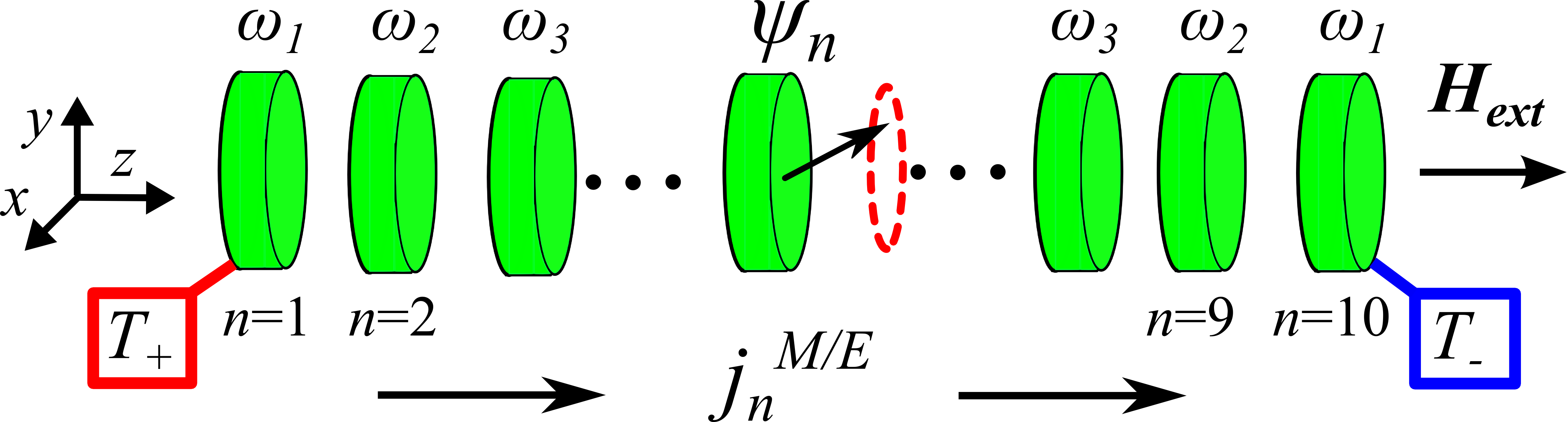
Figure 1: Chain of disks coupled via dipolar interaction. Each disk behaves as a macrospin with precession frequency $\omega_{n}$. The first and last element of each chain are coupled to thermal reservoirs with temperatures $T_{\pm}$, that control the propagation of energy and magnetisation currents.

The dynamics is investigated by means of micromagnetic simulations. The cornerstone of micromagnetism is the Landau-Lifschitz-Gilbert (LLG) equation of motion for a ferromagnet Landau and Lifshitz (1965); Gilbert (2004); Gurevich and Melkov (1996)

$$\dot{\bm{M}}=\gamma{\bm{M}}\times{\bm{H}}_{\rm{eff}}+\frac{\alpha}{M_{s}}{\bm{M}}\times{\dot{\bm{M}}},$$ (1)

which describes the precession of the local magnetisation vector $\bm{M}(\bm{r},t)$ around the effective field ${\bm{H}}_{\rm{eff}}$. The first term of Eq.(1), proportional to the gyromagnetic ratio $\gamma$, accounts for the precession. The second term describes energy dissipation at a rate proportional to the dimensionless Gilbert damping parameter $\alpha$. In the absence of an external driving field, such as thermal fluctuations, spin transfer torque or rf fields, the magnetisation eventually aligns with ${\bm{H}}_{\rm{eff}}$ Gurevich and Melkov (1996); Slavin and Tiberkevich (2009). The saturation magnetisation $M_{s}$ is the norm of the magnetisation vector, which depends on the material and the geometry of the sample. The thermodynamical properties of the system are described by the Gibbs free energy

$$\mathcal{F}= \mu_{0}\int_{V}[A\triangle{\bm{M}}(\bm{r},t)-{\bm{M}}(\bm{r},t)\cdot{\bm{H}}_{\rm{ext}}$$

$$-\frac{1}{2}\bm{M}(\bm{r},t)\cdot\bm{H}_{\rm{dip}}]{\rm{d}}^{3}r,$$ (2)

$\mu_{0}$ being the vacuum magnetic permeability. In the present case, Eq.(II) contains contributions respectively from exchange energy, Zeeman interaction and dipolar interactions. The effective field in Eq.(1) is given by the functional derivative $\bm{H}_{\rm{eff}}=-(1/\mu_{0})\delta\mathcal{F}/\delta\bm{M}$ of the Gibbs free energy with respect to the magnetisation. It is the sum of the following three terms:

$$\bm{H}_{\rm{exc}}= -A\nabla\bm{M}({\bm{r}},t),$$ (3a)

$$\bm{H}_{\rm{ext}}= H\hat{\bm{z}},$$ (3b)

$$\bm{H}_{\rm{dip}}= -\frac{1}{4\pi}\int_{V}\frac{\rho_{M}(\bm{r}-\bm{r}^{\prime})}{|\bm{r}-\bm{r}^{\prime}|^{3}}{\rm{d}}^{3}r^{\prime}+\frac{1}{4\pi}\int_{S}\frac{\sigma_{M}(\bm{r}-\bm{r}^{\prime})}{|\bm{r}-\bm{r}^{\prime}|^{3}}{\rm{d}}^{2}r^{\prime}.$$ (3c)

Eqs. (3a) and (3b) are respectively the exchange field with exchange constant $A$ and the external field with intensity $H$ along $\hat{\bm{z}}$. The exchange field is the short range interaction responsible for the coherent precession of the magnetisation inside each disk, while the applied field defines the precession axis. The dipolar stray field Eq.(3c) contains contributions from the volume charges $\rho_{M}=\nabla\cdot\bm{M}({\bm{r}^{\prime}},t)$ and the surface charges $\sigma_{M}=\bm{M}({\bm{r}^{\prime}},t)\cdot\hat{\bm{n}}$, where $\hat{\bm{n}}$ denotes the normal to the surface of the sample at point $\bm{r}^{\prime}$. The dipolar field acts as a demagnetising field in each disk and adds a coupling between the disks. It is responsible for the nonlinearity of the LLG equation, Eq. (1).

Thermal fluctuations are introduced by adding to the effective field the stochastic term

$${\bm{H}}_{\rm{th}}(\bm{r},t)=\sqrt{DT}(\eta_{x},\eta_{y},\eta_{z}),$$ (4)

where $\eta_{j}(\bm{r},t)$, $j=(x,y,z)$, is a Gaussian random process with zero average and correlation $\left\langle\eta_{j}({\bm{r}},t)\eta_{j^{\prime}}({\bm{r}}^{\prime},t^{\prime})\right\rangle=\delta_{jj^{\prime}}\delta(\bm{r}-\bm{r}^{\prime})\delta(t-t^{\prime})$. Martinez et al. (2007); Grinstein and Koch (2003). The term $T=T(\bm{r})$ denotes the local temperature of the underlying phonon bath, while the coupling strength with the bath is

$$D=\frac{2\alpha k_{B}}{\gamma\mu_{0}V_{M}M_{s}}.$$ (5)

Here $k_{B}$ is the Boltzmann constant and $V_{M}$ is the volume associated to the magnetic moment $\bm{M}(\bm{r})$.

In our micromagnetics simulations, where the sample is represented by a finite element tetrahedral mesh, the LLG equation, Eq. (1), is solved numerically at each mesh node. The coordinate $\bm{r}$ is discretised and corresponds to the positions of the nodes, while $V_{M}$ corresponds the volume of each mesh elements.

III Coupled oscillator model

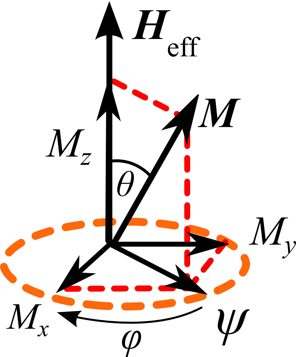
Figure 2: Macrospin $\bm{M}$ precessing around the effective field $\bm{H}_{\rm{eff}}$, described in terms of the stereographic projection $\psi$. The phase $\phi$ describes the dynamics in the $x$-$y$ plane, while the SW power $p=|\psi|^{2}$ is related to the polar angle $\theta$ (see text).

The dynamics of the chain is conveniently described by the volume-averaged magnetisation inside the $n$th disk:

$$\bm{M}^{n}(t)=\frac{1}{V_{n}}\int_{V_{n}}\bm{M}(\bm{r}_{n},t){\mbox{d}}^{3}r_{n}.$$ (6)

Due to the uniform precession of the magnetisation in each disk, the system can be modeled as an assembly of coupled macrospins $\bm{M}_{n}(t)$. With this approximation, Eq.(1) can be written in the form of an equation of motion for an ensemble of coupled nonlinear oscillators Slavin and Tiberkevich (2009)

$$i\dot{\psi}_{n}= \omega_{n}(p_{n})\psi_{n}-i\Gamma_{n}(p_{n})\psi_{n}+\sum_{n^{\prime}}J_{nn^{\prime}}\psi_{n^{\prime}}$$

$$+\sqrt{D_{n}(p_{n})T_{n}}\xi_{n},$$ (7)

where the complex SW amplitudes are defined by

$$\psi_{n}=\frac{M_{x}^{n}-iM_{y}^{n}}{\sqrt{2M_{s}(M_{s}+M_{z}^{n})}}.$$ (8)

By writing Eq.(8) as $\psi_{n}=\sqrt{p_{n}(t)}\mbox{e}^{i\phi_{n}(t)}$, one can see that $\phi_{n}$ describes the precession of $\bm{M}$ in the $x$-$y$ plane, while $p_{n}=|\psi_{n}|^{2}$ (referred to as the local SW power) is related to the polar angle through $\theta_{n}=\arccos(1-p_{n})$, see Fig.2.

The first two terms on the right hand side of Eq.(III) are respectively the nonlinear frequencies $\omega_{n}(p_{n})$ and damping rates $\Gamma_{n}(p_{n})$ of the $n_{\rm{th}}$ disk. Both are proportional to the effective field $\gamma|\bm{H}_{\rm{eff}}^{n}\cdot{\hat{\bm{z}}}|$ acting on each disk.

For the small precession amplitudes considered here, nonlinear effects are taken into account pertubatively by expanding into powers of $p_{n}$ the frequencies and damping rates, respectively as Slavin and Tiberkevich (2009) $\omega_{n}(p_{n})\approx\omega_{n}+\nu p_{n}$, $\Gamma_{n}(p_{n})\approx\alpha\omega_{n}(1+Qp_{n})$. Here $\omega_{n}$, $\nu$ and $Q$ are the coefficients of the expansion of $\omega_{n}(p_{n})$ and $\Gamma_{n}(p_{n})$ to the first order in $p_{n}$. The third term on the right hand side is the interlayer coupling $J_{nn^{\prime}}$. In general it is a complex quantity, and its phase is related to energy gain or dissipation Borlenghi et al. (2014a). In the following we will consider the simple case of a uniform nearest-neighbour interaction that amounts to retain only terms containing $\psi_{n\pm 1}$ in Eq.(III) and set $J_{nn^{\prime}}=J\delta_{n,n\pm 1}$. Note also that the imaginary part of $J_{nn^{\prime}}$ and $\Gamma_{n}$ are related since they both stem from the dissipative term proportional to $\alpha$ in the LLG equation, Eq. (1). Both the nonlinearity and the coupling are due to the dipolar field Eq.(3c). The parameters $(\omega_{n},\nu,Q,J_{nn^{\prime}})$ can be calculated analytically only in some simple cases, but in general they must be inferred from micromagnetic simulations Slavin and Tiberkevich (2009); Naletov et al. (2011).

We consider the case where the temperature is uniform within each disk. In this case, the last term of Eq.(III) describes thermal fluctuations in terms of the complex Gaussian random variables $\xi_{n}=(\eta_{x}^{n}+i\eta_{y}^{n})$ and the nonlinear diffusion constant $D_{n}(p_{n})$. In the linear regime, the latter equals $\gamma D$, where $D$ is the quantity defined in Eq.(5). In the nonlinear regime $D_{n}(p_{n})$ depends on $\Gamma_{n}(p_{n})$, $\omega_{n}(p_{n})$ and $J_{nn^{\prime}}$ and must be fixed consistently to satisfy the fluctuation-dissipation theorem. For the single oscillator this amounts to fix $D_{n}(p_{n})\propto\Gamma_{n}(p_{n})/\omega_{n}(p_{n})$Slavin and Tiberkevich (2009). This is necessary to ensure that, for $T_{n}\equiv T$, the systems approaches a global canonical equilibrium at temperature $T$. Consistently with the small-amplitude limit, we assume $\Gamma_{n}(p_{n})=\alpha\omega_{n}(p_{n})$. As a consequence, the noise term in Eq.(III) becomes purely additive and $D_{n}(p_{n})$ reduces to a constant $D=\alpha$ in units with $k_{B}=1$.

Taking into account the above approximations, we simplify Eq.(III) into

$$i\dot{\psi}_{n}= (1+i\alpha)\left[-\nu|\psi_{n}|^{2}\psi_{n}-\omega_{n}\psi_{n}-J(\psi_{n+1}+\psi_{n-1})\right]$$

$$+\sqrt{\alpha T_{n}}\,\xi_{n}(t)\quad.$$ (9)

Upon defining the “Hamiltonian”

$$\mathcal{H}={\sum_{n}}[{\omega_{n}|\psi_{n}|^{2}+\frac{\nu}{2}|\psi_{n}|^{4}+J(\psi_{n}^{*}\psi_{n+1}+\psi_{n}\psi_{n+1}^{*})}],$$ (10)

where $(\psi_{n},i\psi_{n}^{*})$ are canonically conjugate variables satisfying the Hamilton equations $\dot{\psi}_{n}=-\partial\mathcal{H}/\partial i\psi_{n}^{*}$, Eq.(9) can be written more concisely in the form of a Langevin equation with uniform bath coupling $\alpha$

$$i\dot{\psi}_{n}=-(1+i\alpha)\frac{\partial\mathcal{H}}{\partial\psi_{n}^{*}}+\sqrt{\alpha T_{n}}\,\xi_{n}.$$

In the absence of coupling with the external baths $(\alpha=0)$, Eq.(9) is the well-known DNLS equation Eilbeck et al. (1985) which, at variance with its continuum limit, is not integrable Rumpf and Newell (2003). Such equation describes a large class of conservative oscillating systems. Some examples include transport in biomolecules, Bose-Einstein condensates in optical lattices, mechanical oscillators and photonics waveguides Eilbeck and Johansson (2003); Kevrekidis (2009). The dependence of $\omega_{n}$ on the lattice sites introduces an heterogeneity that is also connected with the nonlinear version of the Anderson tight-binding model Pikovsky and Shepelyansky (2008); Kopidakis et al. (2008); Basko (2011).

In the non dissipative limit, the model admits a further constant of motion besides energy, namely, the total SW power $\mathcal{P}=\sum_{n}p_{n}$. As a consequence, the thermodynamic equilibrium phase-diagram is two-dimensional, and each equilibrium state is determined by the energy density $\mathcal{H}/N$ and the SW density $\mathcal{P}/N$  Rasmussen et al. (2000).

In the nonequilibrium regime, the local fluxes of the conserved quantities are of special interest. By computing the time derivatives of the SW power $p_{n}$ and of the local energy $\mathcal{H}_{n}$, one obtains the two continuity equations Slavin and Tiberkevich (2009); Iubini et al. (2013); Borlenghi et al. (2014b, c, a)

$$\dot{p}_{n}= \mathcal{J}^{M}_{n}+j_{n+1}^{M}-j_{n}^{M},$$ (11a)

$$\dot{\mathcal{H}}_{n}= \mathcal{J}^{E}_{n}+j_{n+1}^{E}-j_{n}^{E},$$ (11b)

where

$$j_{n}^{M}= 2J\,{\rm{Im}}[\psi_{n}^{*}(\psi_{n+1}-\psi_{n})],$$ (12a)

$$j_{n}^{E}= 2J\,{\rm{Re}}\left[\frac{\partial\mathcal{H}}{\partial i\psi_{n}}(\psi_{n+1}-\psi_{n})\right].$$ (12b)

are the magnetisation and energy currents associated with the hamiltonian coupling between neighboring oscillators. The remaining terms $\mathcal{J}^{M}_{n}$ and $\mathcal{J}^{E}_{n}$ account for the exchange with the reservoirs due to both fluctuations and damping. Their steady-state averages are computed using stochastic calculus, by evaluating the change of $p_{n}$ and $\mathcal{H}_{n}$ up to second order in the noise term Lepri et al. (2003). As a result, one gets

$$\langle\mathcal{J}^{M}_{n}\rangle=2\alpha T_{n}-2\alpha\left\langle\left[\omega_{n}(p_{n})p_{n}+J{\rm{Re}}\left(\psi_{n}^{*}(\psi_{n+1}+\psi_{n-1}\right)\right]\right\rangle\\$$ (13)

A similar (but more involved) expression holds for the energy fluxes. As a preliminary test, we verified that for a generic nonequilibrium stationary state the above definitions of fluxes satisfy the local flux balance expressed in Eqs. (11a) and (11b).

For a system which is driven out-of-equilibrium from its boundaries, the local temperature represents a useful observable for the characterisation of the stationary state. Note in particular that the quantity $T_{n}$ that appears in Eq.(III) specifies the temperature of the phonon bath, which in general does not correspond to the temperature of the system Iubini et al. (2012). The definition of temperature for a system of interacting magnetic moments is not straightforward, since the model Hamiltonian is non separable, and one cannot relate temperature to the average kinetic energy. Within the DNLS formalism, one can use the general microcanonical definition of temperature for non separable Hamiltonians with two conserved quantities Franzosi (2011). The general expression is nonlocal and rather involved, we refer to Refs.Franzosi (2011); Iubini et al. (2012, 2013) for details. Since we are interested in the limit of low temperatures and low amplitudes, we can follow the derivation in Ref. Iubini et al. (2013) and introduce a simple approximation of the microcanonical temperature based on a mapping of the DNLS equation to a chain of nonlinear coupled rotators (XY model). Accordingly, the temperature is approximated by

$$T_{XY}=f(\left\langle p_{n}\right\rangle)\left[\left\langle\dot{\phi}_{n}^{2}\right\rangle-\left\langle\dot{\phi}_{n}\right\rangle^{2}\right],$$ (14)

and it acquires a simple interpretation of the phase-fluctuations of the oscillator $\psi_{n}$. The function $f(\left\langle p_{n}\right\rangle)$ is a rescaling factor that depends on the average local power $\left\langle p_{n}\right\rangle$. One can also show that for $\left\langle p_{n}\right\rangle\ll 1$, $f(\left\langle p_{n}\right\rangle)=2\left\langle p_{n}\right\rangle$.

IV Micromagnetic simulations

The micromagnetic simulations were performed with the Nmag software Fischbacher et al. (2007), using a tetrahedral finite element mesh with maximum size of 3 nm, of the order of the Py exchange length, and an integration time step is 1 ps. The mesh was automatically generated by the Netgen package Schöberl (1997).

Each disk of the chain has thickness $t=3$ nm, radius $R=20$ nm, and an interlayer distance $d=3$ nm. The applied field $\bm{H}_{\rm{ext}}=1$T defines the precession axis of the magnetisation along $\hat{\bm{z}}$. The exchange stiffness $A=1\times 10^{-11}$ J/m corresponds to that of Py, while the other micromagnetic parameters are $M_{s}=0.94$ T/$\mu_{0}$, $\alpha=8\times 10^{-3}$ and $\gamma=1.873\times 10^{11}$ rad$\times$s^-1 $\times$T^-1.

The output of the simulations consists of the ensemble of the magnetisation vectors $\left\{\bm{M}^{n}({\bm{r}}_{n},t)\right\}$, $n=1,...,10$. Each vector depends on the spacial coordinate ${\bm{r}}_{n}$ inside the $n_{\rm{th}}$ disk, and the collective magnetisation dynamics of each disk is given by the volume average Eq.(6) Slavin and Tiberkevich (2009); Borlenghi et al. (2014c)

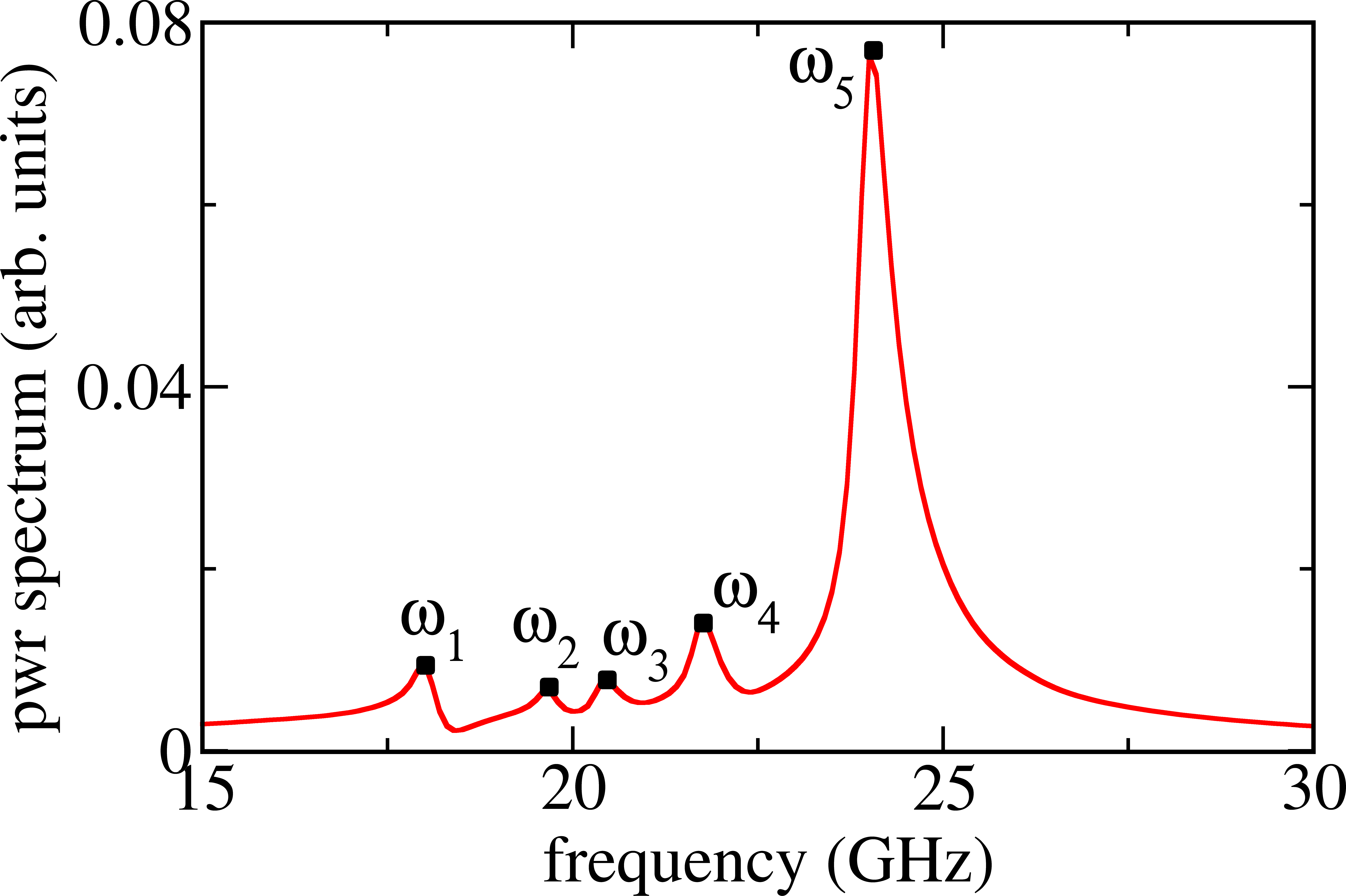
Figure 3: SW spectrum of the system at zero temperature, characterised by 5 dipolar modes.

To have a basis for comparison, we consider first dynamics at zero temperature. Starting with the magnetization uniformly tilted 5 with respect to the z axis, the time evolution is computed for 30 ns. The SW power spectrum, shown in Fig.3, is given by the absolute value of the Fourier transform of the collective variable $\Psi(t)=\sum_{n=1}^{10}\psi_{n}(t)$. The spectrum consists of five dipolar modes with frequencies $(\omega_{1},...,\omega_{5})$ of respectively $(18,19.7,20.5,21.8,24)$ GHz. By inspecting the spectra of the individual disks, one can see that the mode $\omega_{1}$ corresponds to the precession of the first and tenth disks, the mode $\omega_{2}$ to the second and ninth disks and so on until the fifth disk which precesses with frequency $\omega_{5}$, see Fig.(1). This indicates that the system has a mirror symmetry around its center, due to the fact that each disk behaves as a magnetic dipole. Aligning those dipoles in a chain gives a structure where the intensity of the dipolar field, which controls the frequencies, is symmetric around the center of the chain.

Let us now discuss the off equilibrium dynamics. We consider the configuration normally adopted to study heat transfer in chains of nonlinear oscillators Lepri et al. (2003), where the thermal baths act only at the boundaries of the system. This setup is different from the usual micromagnetic studies of the spin-Seebeck effect Ohe et al. (2011); Hinzke and Nowak (2011); Ritzmann et al. (2014); Etesami et al. (2014), where each spin is coupled to a thermal reservoir with a different temperature. The main advantage of our choice consists in that it allows to observe the spontaneous thermalisation of the system, by probing the XY temperature defined in Eq.(14), for the spins that are not directly connected to the thermal baths. Experimentally, this could be realised by separating the disks with thermal insulating spacers, so that energy flows are carried only by the dipolar coupling.

The simulations at finite temperature were performed starting with the magnetisation aligned along $\hat{\bm{z}}$ and evolving the system in the presence of the thermal baths for 110 ns. The relevant observables were computed after an interval of 70 ns, necessary for the system to reach the nonequilibrium steady state. The results were time averaged over the last 40 ns and then ensemble averaged over 32 samples with different realisation of the thermal noise.

The high temperature bath $T_{+}$ ranges between 5 and 30 K, while the lower temperature bath $T_{-}$ is kept fix at 5 K, so that $\Delta T=T_{+}-T_{-}$ is comprised between 0 and 25 K. The local currents are always expressed per unit coupling and are thus pure numbers. According to our convention, $j_{n}^{M/E}$ refers to the current propagating from disk $n$ to disk $n+1$ and positive (resp. negative) currents propagate from left to right (resp. from right to left).

Figure 4: Profiles of magnetisation (a) and energy (b) currents computed for different values of $\Delta T$. The profiles are symmetric for $\Delta T=0$, and then become strongly asymmetric. The lines are guide to the eye.

Figure 5: Profiles of the magnetisation currents for $T_{-}=0$ K and different values of $T_{+}$. The right-going current decreases exponentially along the chain. The dashed lines are fit with $A{\rm{e}}^{-x/x_{0}}$, for different values of the parameters $(A,x_{0})$. The energy currents have similar profiles (not reported).

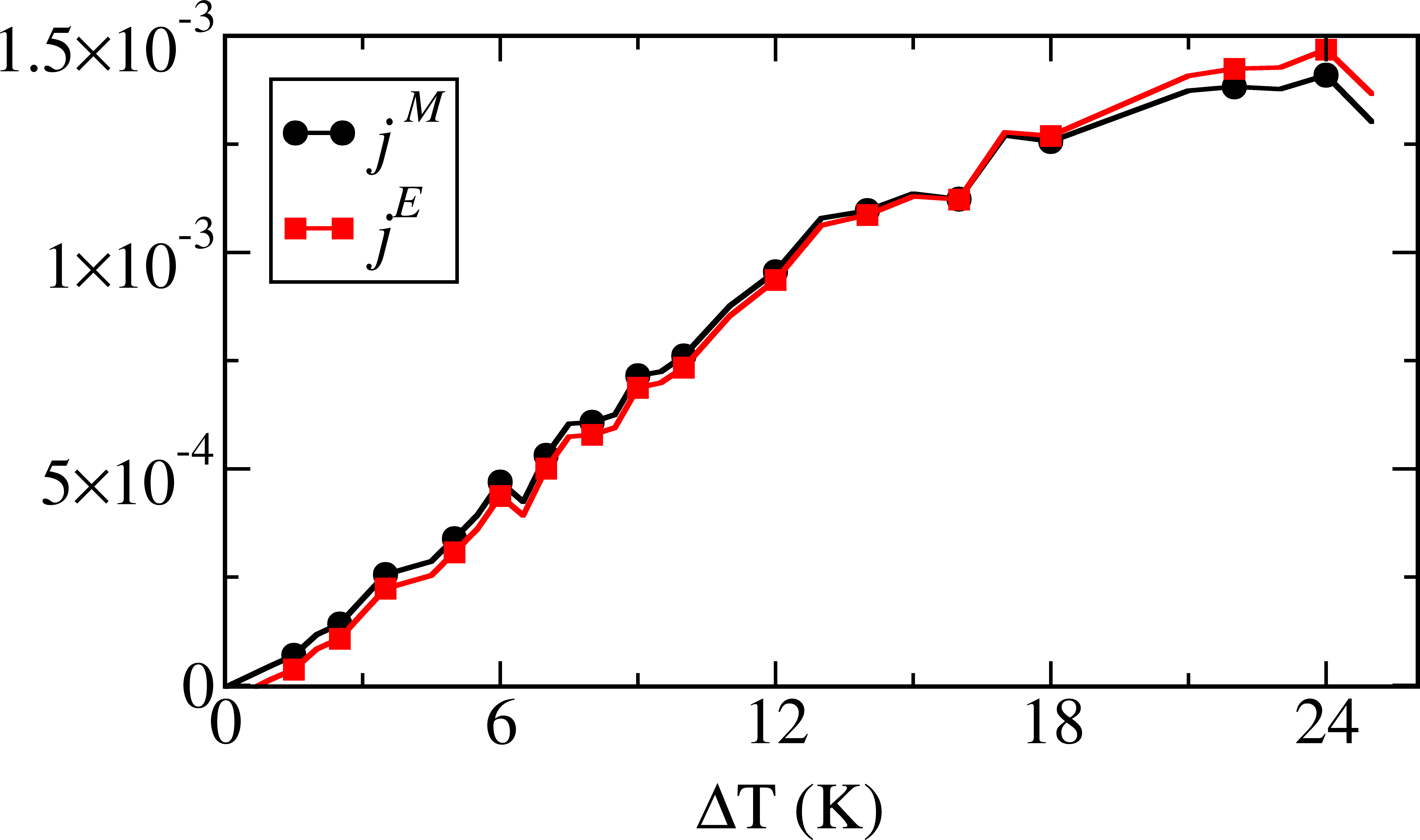
Figure 6: Currents $j^{M/E}=j_{1}^{M/E}+j_{9}^{M/E}$ injected from the reservoirs vs the temperature difference $\Delta T$. The currents grow linearly with $\Delta T$ in the low temperature regime, and then reach a plateau. The lines are guides to the eye.

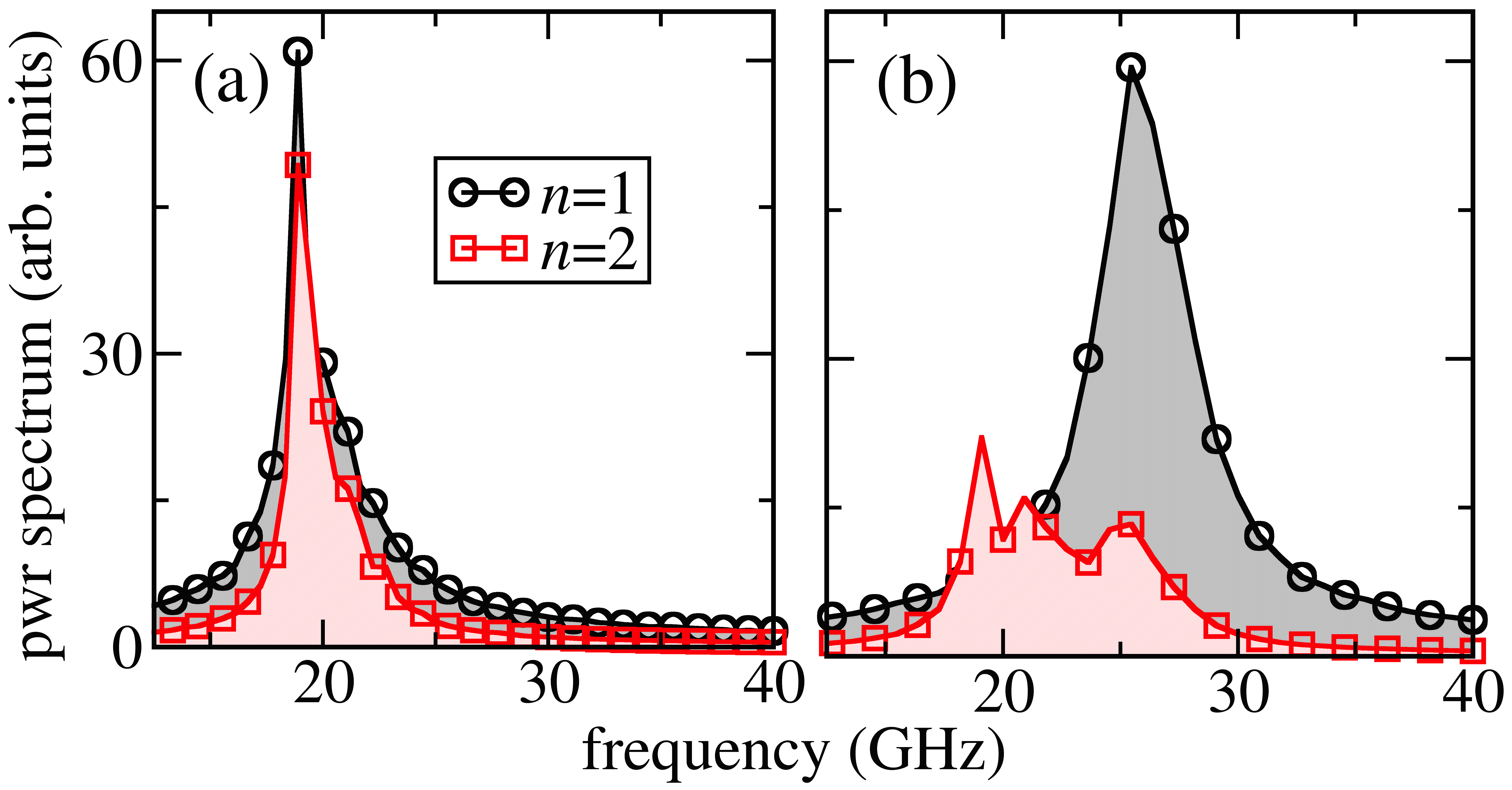
Figure 7: Finite temperature power spectra of disks 1 and 2. (a) At low temperatures ($T\pm=5$ K) regime the peaks overlap and the currents are proportional to $\Delta T$. (b) At high temperature ($T_{+}=30$ K) the spectrum of disk 1 shifts towards high frequency, reducing its overlap with disk 2. In this condition, the current does not increase anymore with $\Delta T$.

In contrast to previous studies of the off-equilibrium DNLS, here the dissipation is both at the edges and in the bulk of the system. As a consequence, the currents do not have a flat profile in the bulk, but decrease exponentially along the chain. In the thermodynamic limit, this system is thus an insulator.

Figs.4 (a) and (b) show respectively the profiles of magnetisation and energy currents, for different values of $\Delta T$. The two currents have similar profiles, and they do not vanish when $\Delta T=0$ (black dots). In both cases, they are symmetric with respect to the zero-current axis. This behaviour is due to the fact that the currents generated by the two baths travel in opposite directions and decrease because of the damping, vanishng in the middle of the chain. Note that, although the local currents do not vanish at equilibrium, the total current is zero. Increasing $T_{+}$ leads to the increase of the right-going currents, and moves the point where the local currents vanish.

In all these cases, the system behaves essentially as sink: the currents injected from the baths are dissipated in the bulk, so that there is no net transport. A situation where transport occurs can be observed in Fig.(5), which shows the case where $T_{-}=0$ and (the right-going) current is injected only by $T_{+}$. The current decreases exponentially, and for high enough value of $\Delta T$ remains positive until the end of the system. Note that in the thermodynamic limit this system is an insulator, due to the damping in the bulk.

Note that the local currents do not grow indefinitely with $\Delta T$, but they saturates around $\Delta T\approx 20$ K. This can be seen more clearly in Fig.6, where the currents injected from the reservoirs $j^{M/E}=j_{1}^{M/E}+j_{9}^{M/E}$ grow linearly with $\Delta T$ until they reach a plateau for $\Delta T\approx 20$ K.

This phenomenon originates from the fact that the LLG equation is nonlinear, and consequently the frequency spectrum of the system is temperature dependent. Fig. 7 shows the power spectra of the disks 1 and 2. Panel (a) displays the low temperature regime, with $T_{+}=T_{-}=5$ K. Thermal fluctuations excite all the modes of the system, and both disks display a broad peak between 17 and 25 GHz. The current increases linearly with $\Delta T$ as far those peaks overlap. Panels (b) show the high temperature case, where disk 1, directly connected to the hot bath, increases its frequency and does not overlap with disk 2. This situation is a manifestation of stochastic phase synchronisation (that is, the control of synchronisation through temperature) in the propagation of heat current. A similar mechanism is at the basis of spin and thermal rectifiers Li et al. (2004); Ren and Zhu (2013); Ren et al. (2014); Borlenghi et al. (2014b, c).

The profile of the local SW powers $p_{n}$ is displayed in Fig.8 (a). The powers reach the maximum at the edges, directly connected to the baths, and decay along the chain. As expected, their profile is symmetric for $\Delta T=0$, and becomes strongly asymmetric when the temperature difference is finite. Note that the powers increase with with temperature until $\Delta T\approx 15$ K and then remain roughly constant. In this high temperature regime, $p_{1}$ keeps increasing because of thermal fluctuations, but $p_{2}$ decreases. This is due to the fact that energy remains confined in the first disk due to the de-synchronization, as previously discussed.

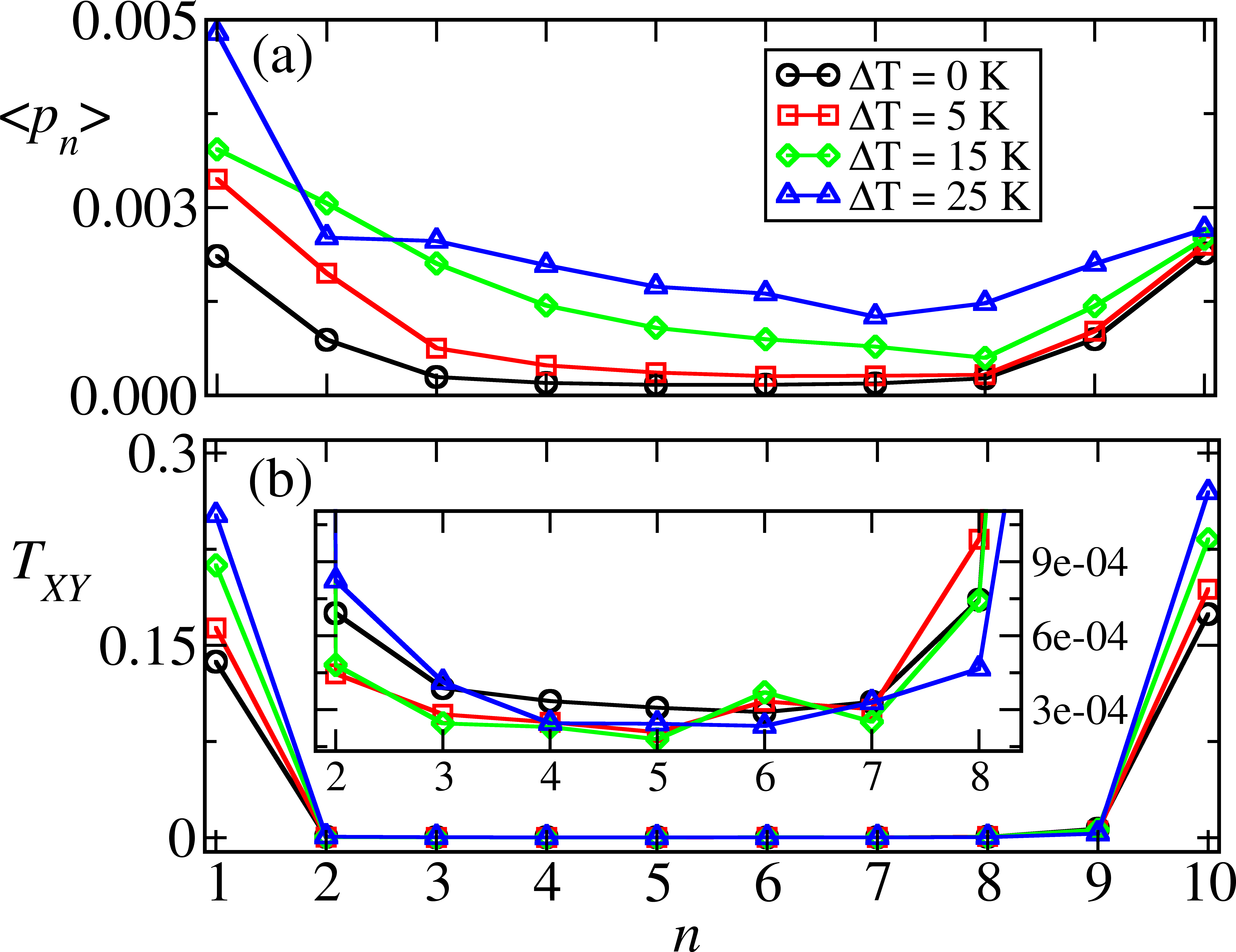
Figure 8: (a) Profiles of SW powers $p_{n}$ for different values of $\Delta T$. (b) Profiles of spin temperature $T_{XY}$ for different values of $\Delta T$. The inset displays a magnification of the profiles between the disks 2 and 8, which show the spontaneous thermalisation of the chain. The lines are guide to the eye.

Fig.8(b) shows the spin temperature profiles $T_{XY}$ of the chain, computed for different values of $\Delta T$. The temperature is higher at the boundaries, where phase fluctuations are given by the direct contact with the baths, and then decreases dramatically towards the center of the chain, as can be seen from the inset.

V comparison with the oscillator model

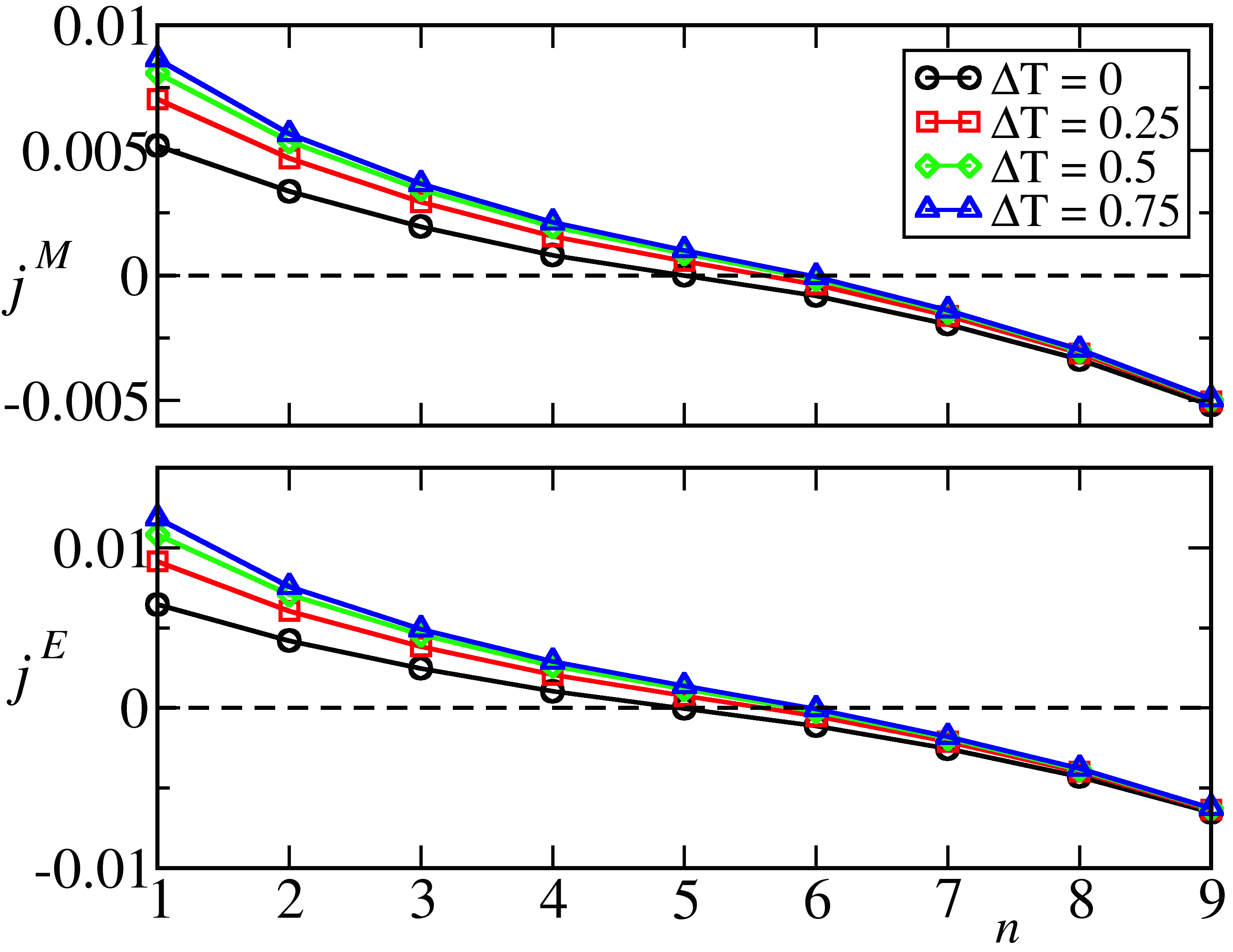
Figure 9: Simulation of Eq. (9) with $J=0.1$, $\alpha=0.008$, $\nu=1$, $(\omega_{1},\omega_{2},\omega_{3},\omega_{4},\omega_{5})=(1,1.09,1.15,1.21,1.33)$ and different applied temperature differences $\Delta T$ . The temperature of the leftmost reservoir spaces in the interval $T_{+}=[0.5\,,\,1.25]$, while the rightmost one is kept fixed at $T_{-}=0.5$.

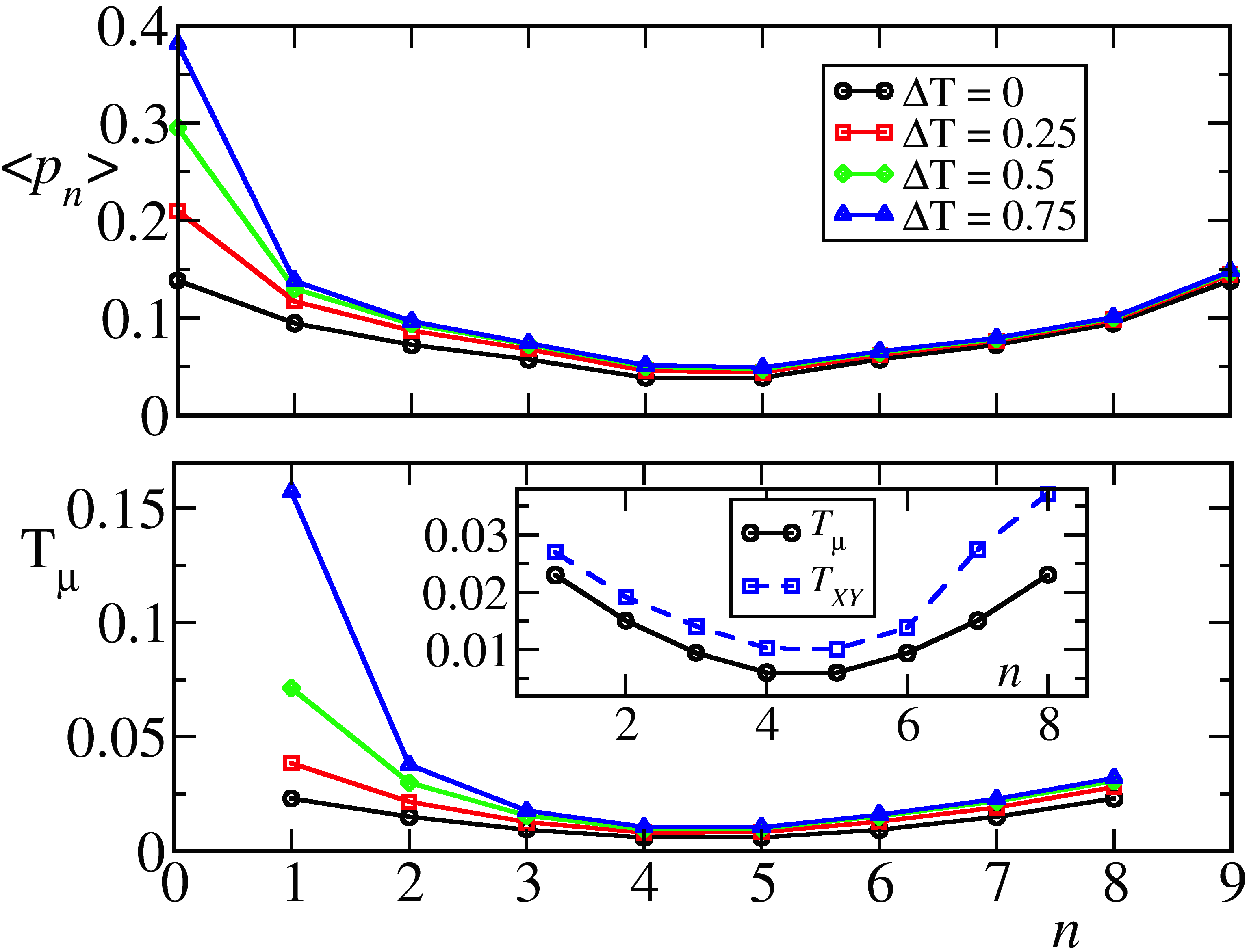
Figure 10: Simulation of Eq. (9), SW profiles and microcanonical temperature $T_{\mu}$ for different applied temperature differences $\Delta T$. The parameters of the simulation are the same as in Fig. 9. For each lattice site $n$, the local temperature $T_{\mu}$ is calculated by evaluating the general definition Iubini et al. (2012, 2013) on a triplet of sites centered around $n$. The inset of the lower panel shows a comparison between $T_{\mu}$ and $T_{XY}$ for the profile with $\Delta T=0$.

The micromagnetic simulations indicate that the system has some form of mirror symmetry around its center. Thus we model this by choosing the linear frequencies in model (9) such that $\omega_{n}^{0}=\omega_{N-n}^{0}$. A relatively small coupling $J=0.1$ has been employed. As in Section IV, the fluctuating forces are applied only at the boundaries of the system, i.e. we choose $T_{n}=[T_{+}\delta_{n,1}+T_{-}\delta_{n,N}]$;

As a test for stationarity we evaluated the average currents from the heat baths $\sum_{n}\langle\mathcal{J}_{n}^{M}\rangle$ and $\sum_{n}\langle\mathcal{J}_{n}^{H}\rangle$ are indeed vanishing within statistical accuracy.

In Figs. 9 and 10 we show the current and SW power profiles along the chain. Comparing with the corresponding figures 4(a,b) and 8(a), the qualitative agreement is good. The lower panel of Fig. 10 reports the temperature profiles $T_{\mu}$ calculated with the exact microcanonical expression defined in Refs.Iubini et al. (2012, 2013). Such profiles are in good agreement with the phase temperature $T_{XY}$ (see the inset) and qualitatively reproduce the temperature profiles calculated within the micromagnetic framework in Fig. 2. Altogether, this confirms that definition (14) is a sensible approximation in the present setup.

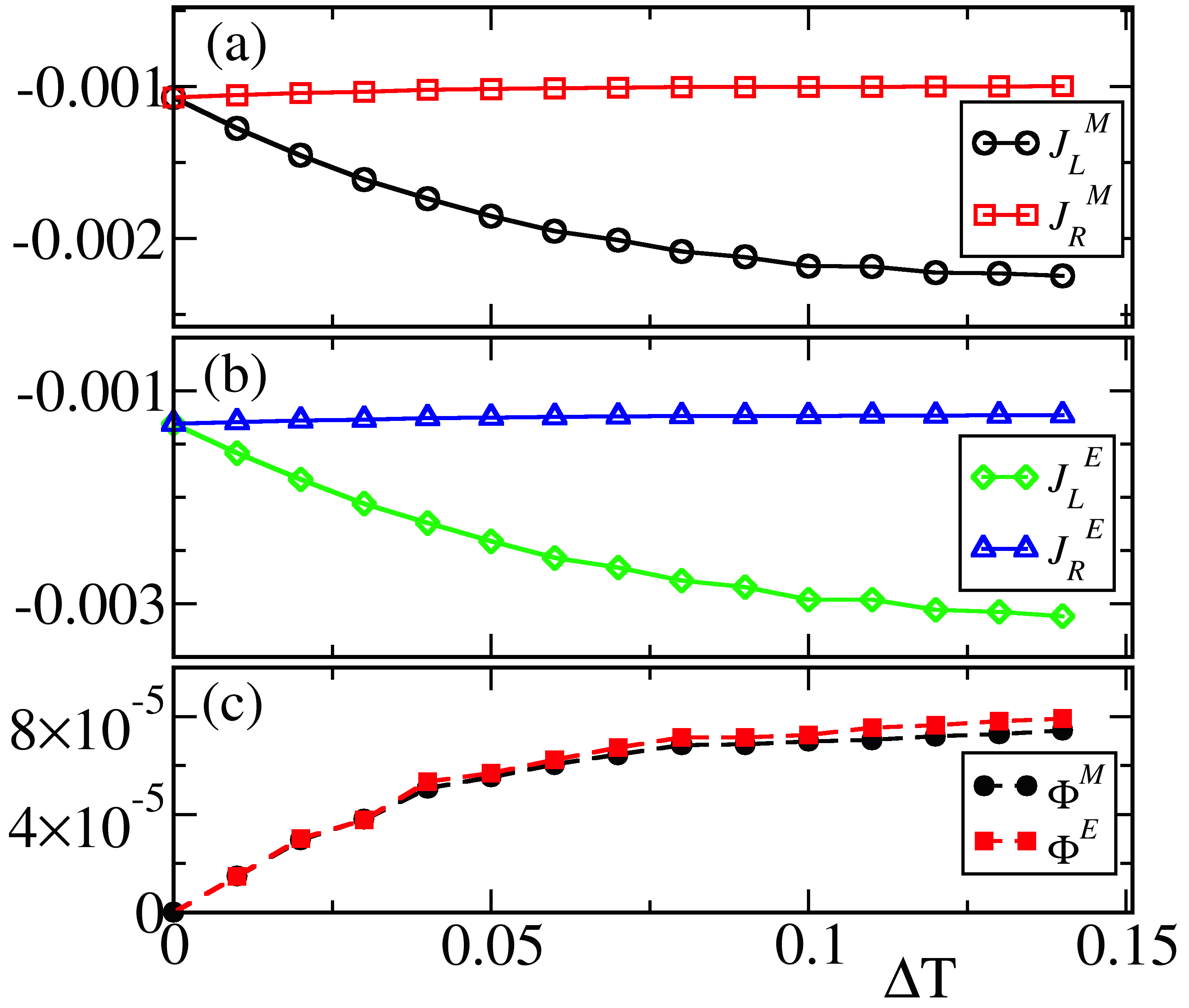
Figure 11: Simulation of Eq. (9) Boundary magnetisation (a) and energy (b) currents toward the two left and right reservoirs versus the temperature difference $\Delta T$ for $T_{-}=0.05$, other parameters given in the text. Panel (c) shows the corresponding excess fluxes calculated with Eq.(15).

Finally, in panels (a) and (b) of Fig.11 we show the stationary boundary fluxes $\mathcal{J}^{M}_{n}$ and $\mathcal{J}^{E}_{n}$. Nicely, they reproduce the saturation effect observed in Fig.4 with the micromagnetic simulations. It should be noted that the currents do not vanish for $\Delta T=0$: this is simply because the system is off-equilibrium also in this case due to the presence of the dissipation in the bulk of the chain. For the very same reason, the two currents flowing at the boundary are not equal. In order to single out the purely transport contribution from the dissipative one in the boundary fluxes, we define an excess boundary flux $\Phi^{M,E}$ as

$$\Phi^{M,E}=\mathcal{J}_{R}^{M,E}(\Delta T)-\mathcal{J}_{R}^{M,E}(0)\quad,$$ (15)

that takes into account the amount of magnetisation/energy which is transported per unit time with respect to the purely dissipative symmetric profile at $\Delta T=0$. The behaviour of $\Phi^{M,E}(\Delta T)$ is shown in Fig.11(c). Both the excess fluxes have positive sign, meaning that there is a net transport of energy and magnetisation from left to right. Moreover they show the same saturation effect observed in panels (a) and (b).

VI conclusions

In this work we have illustrated the spin-Seebeck effect in a small array of coupled magnetic nanodisks and we have related to general transport properties of out-of-equilibrium chains of nonlinear oscillators. The dynamics of the disk chain has been investigated by means of micromagnetic simulations and compared with the effective model, Eq. (9). There is indeed a good qualitative agreement between the two approaches, and a good physical insight can be achieved from the coupled oscillator model.

Another remarkable result, is that the relationship with the XY model provides a simple prescription for computing the local phase temperature in the micromagnetic simulations via Eq. (14). Such observable plays a relevant role in our setup, since it allows to quantify thermal fluctuations inside the system, i.e. for macrospins that are not directly connected to the external reservoirs. This last issue is of major importance for non-standard Hamiltonians like the DNLS one, where kinetic and potential energies are not separated. Indeed, the XY approximation allows introducing the simple kinetic expression $T_{XY}$ for the temperature, that can safely approximate the microcanonical one $T_{\mu}$. This is of practical importance, considering that the microscopic definitions of $T$ and $\mu$ are pretty much involved for a non separable Hamiltonian, like the DNLS one.

The presence of two coupled currents is related to the existence of two thermodynamic forces Onsager (1931a, b); M. Toda (1983) $(\Delta T,\Delta\mu)$, the latter being the difference of chemical potential Iubini et al. (2012, 2013). In this work we limited to the case where $\Delta\mu=0$. Actually, chemical potential gradients can be easily accounted for within the DNLS language, by adding terms of the form $i\alpha\mu_{n}\psi_{n}$ to Eq.9 Iubini et al. (2013). For our system of precessing spins, this is interpreted as a torque that compensates the damping and controls the magnon relaxation time towards the reservoirs Iubini et al. (2012, 2013); Borlenghi et al. (2014c). This can be experimentally realised trough spin transfer torque Slonczewski (1996); Berger (1996); Slavin and Tiberkevich (2009). In this case the spin-torque induces a nonequilibrium dynamics and may lead to self-sustained oscillations, thus opening a new realm of transport phenomena. We plan to investigate those setups in the next future.

References

- Lepri et al. (2003) S. Lepri, R. Livi, and A. Politi, Phys. Rep. 377, 1 (2003).
- Basile et al. (2007) G. Basile, L. Delfini, S. Lepri, R. Livi, S. Olla, and A. Politi, Eur. Phys J.-Special Topics 151, 85 (2007).
- Dhar (2008) A. Dhar, Adv. Phys. 57, 457 (2008).
- Saito et al. (2010) K. Saito, G. Benenti, and G. Casati, Chem. Phys. 375, 508 (2010).
- Uchida et al. (2008) K. Uchida et al., Nature 455, 778 (2008).
- Uchida et al. (2010) K. Uchida et al., Nat. Mater. 9, 894 (2010).
- Bauer et al. (2012) G. E. W. Bauer, E. Saitoh, and B. J. van Wees, Nat. Mater. 11, 391 (2012).
- Ohe et al. (2011) J.-i. Ohe, H. Adachi, S. Takahashi, and S. Maekawa, Phys. Rev. B 83, 115118 (2011).
- Hinzke and Nowak (2011) D. Hinzke and U. Nowak, Phys. Rev. Lett. 107, 027205 (2011).
- Ritzmann et al. (2014) U. Ritzmann, D. Hinzke, and U. Nowak, Phys. Rev. B 89, 024409 (2014).
- Etesami et al. (2014) S. R. Etesami, L. Chotorlishvili, A. Sukhov, and J. Berakdar, Phys. Rev. B 90, 014410 (2014).
- Savin et al. (2005) A. Savin, G. Tsironis, and X. Zotos, Phys. Rev. B 72, 140402 (2005).
- Bagchi and Mohanty (2012) D. Bagchi and P. Mohanty, Phys. Rev. B 86, 214302 (2012).
- Basko (2011) D. Basko, Annals of Physics 326, 1577 (2011).
- Iubini et al. (2012) S. Iubini, S. Lepri, and A. Politi, Phys. Rev. E 86, 011108 (2012).
- De Roeck and Huveneers (2014) W. De Roeck and F. Huveneers, Commun. Pure Appl. Math. (2014).
- Iubini et al. (2013) S. Iubini, S. Lepri, R. Livi, and A. Politi, J. Stat. Mech. p. P08017 (2013).
- Borlenghi et al. (2014a) S. Borlenghi, S. Iubini, S. Lepri, L. Bergqvist, A. Delin, and J. Fransson, arXiv:1411.5170 (2014a).
- Landau and Lifshitz (1965) L. D. Landau and E. M. Lifshitz, in Collected papers (Ed. Pergamon, 1965).
- Gilbert (2004) T. Gilbert, IEEE, Transaction on Magnetics 40, 3443 (2004).
- Gurevich and Melkov (1996) A. G. Gurevich and G. A. Melkov, Magnetization Oscillation and Waves (CRC Press, 1996).
- Slavin and Tiberkevich (2009) A. Slavin and V. Tiberkevich, IEEE Transactions on Magnetics 45, 1875 (2009).
- Martinez et al. (2007) E. Martinez et al., Phys. Rev. B 75, 174409 (2007).
- Grinstein and Koch (2003) G. Grinstein and R. H. Koch, Phys. Rev. Lett. 90, 207201 (2003).
- Naletov et al. (2011) V. V. Naletov et al., Phys. Rev. B 84, 224423 (2011).
- Eilbeck et al. (1985) J. C. Eilbeck, P. S. Lomdahl, and A. C. Scott, Physica D 16, 318 (1985).
- Rumpf and Newell (2003) B. Rumpf and A. C. Newell, Physica D: Nonlinear Phenomena 184, 162 (2003).
- Eilbeck and Johansson (2003) J. C. Eilbeck and M. Johansson, in Conference on Localization and Energy Transfer in Nonlinear Systems (2003), p. 44.
- Kevrekidis (2009) P. G. Kevrekidis, The Discrete Nonlinear Schrödinger Equation (Springer Verlag, Berlin, 2009).
- Pikovsky and Shepelyansky (2008) A. S. Pikovsky and D. L. Shepelyansky, Phys. Rev. Lett. 100, 094101 (2008).
- Kopidakis et al. (2008) G. Kopidakis, S. Komineas, S. Flach, and S. Aubry, Phys. Rev. Lett. 100, 084103 (2008).
- Rasmussen et al. (2000) K. Rasmussen, T. Cretegny, P. G. Kevrekidis, and N. Grønbech-Jensen, Phys. Rev. Lett. 84, 3740 (2000).
- Borlenghi et al. (2014b) S. Borlenghi, W. Wang, H. Fangohr, L. Bergqvist, and A. Delin, Phys. Rev. Lett. 112, 047203 (2014b).
- Borlenghi et al. (2014c) S. Borlenghi, S. Lepri, L. Bergqvist, and A. Delin, Phys. Rev. B 89, 054428 (2014c).
- Franzosi (2011) R. Franzosi, J. Stat. Phys 143, 824 (2011).
- Fischbacher et al. (2007) T. Fischbacher et al., Magnetics, IEEE Transactions on 43, 2896 (2007).
- Schöberl (1997) J. Schöberl, Computing and Visualization in Science 1, 41 (1997).
- Li et al. (2004) B. Li, L. Wang, and G. Casati, Phys. Rev. Lett. 93, 184301 (2004).
- Ren and Zhu (2013) J. Ren and J.-X. Zhu, Phys. Rev. B 88, 094427 (2013).
- Ren et al. (2014) J. Ren, J. Fransson, and J.-X. Zhu, Phys. Rev. B 89, 214407 (2014).
- Onsager (1931a) L. Onsager, Phys. Rev. 37, 405 (1931a).
- Onsager (1931b) L. Onsager, Phys. Rev. 38, 2265 (1931b).
- M. Toda (1983) N. S. M. Toda, R. Kubo, Statistical physics (Springer-Verlag, 1983).
- Slonczewski (1996) J. Slonczewski, Journal of Magnetism and Magnetic Materials 159, L1 (1996), ISSN 0304-8853.
- Berger (1996) L. Berger, Phys. Rev. B 54, 9353 (1996).